
Ordering of Omics Features Using Beta Distributions on Montecarlo p-Values


1
Centro de Excelencia de Modelación y Computación Científica, Universidad de La Frontera, Temuco 01145, Chile
2
Department of Statistics and Operation Research, Faculty of Mathematics, Universitat de Valencia, 46100 Burjasot, Spain
3
Department of Computer Science, ETSE, Universitat de Valencia, Avda. de la Universidad, s/n, 46100 Burjasot, Spain
*
Author to whom correspondence should be addressed.
Mathematics 2021, 9(11), 1307; https://doi.org/10.3390/math9111307
Submission received: 4 May 2021
/
Revised: 30 May 2021
/
Accepted: 4 June 2021
/
Published: 7 June 2021
(This article belongs to the Special Issue Models and Methods in Bioinformatics: Theory and Applications)
Abstract
:The current trend in genetic research is the study of omics data as a whole, either combining studies or omics techniques. This raises the need for new robust statistical methods that can integrate and order the relevant biological information. A good way to approach the problem is to order the features studied according to the different kinds of data so a key point is to associate good values to the features that permit us a good sorting of them. These values are usually the p-values corresponding to a hypothesis which has been tested for each feature studied. The Montecarlo method is certainly one of the most robust methods for hypothesis testing. However, a large number of simulations is needed to obtain a reliable p-value, so the method becomes computationally infeasible in many situations. We propose a new way to order genes according to their differential features by using a score defined from a beta distribution fitted to the generated p-values. Our approach has been tested using simulated data and colorectal cancer datasets from Infinium methylationEPIC array, Affymetrix gene expression array and Illumina RNA-seq platforms. The results show that this approach allows a proper ordering of genes using a number of simulations much lower than with the Montecarlo method. Furthermore, the score can be interpreted as an estimated p-value and compared with Montecarlo and other approaches like the p-value of the moderated t-tests. We have also identified a new expression pattern of eighteen genes common to all colorectal cancer microarrays, i.e., 21 datasets. Thus, the proposed method is effective for obtaining biological results using different datasets. Our score shows a slightly smaller type I error for small sizes than the Montecarlo p-value. The type II error of Montecarlo p-value is lower than the one obtained with the proposed score and with a moderated p-value, but these differences are highly reduced for larger sample sizes and higher false discovery rates. Similar performances from type I and II errors and the score enable a clear ordering of the features being evaluated.
1. Introduction
A major aim in most omics analyses is to order the genes according to their biological relevance with respect to a biological phenomenon [1,2]. To do so, experimental studies are designed and performed but usually the number of available samples in these studies is much lower than the number of expressed features (genes, methylation, etc.). In statistical terms, the number of variables is much higher than the sample size. We have a large number of hypotheses to be tested and distributional hypotheses about these features are not tenable i.e., the null distribution of the statistics is unknown. A common approach to tackle this problem resorts to randomization methods where different realizations of this randomization distribution are generated and, from them, a Montecarlo p-value is obtained [3,4,5,6]. Then these p-values are simply ordered or compared with a given threshold. These randomization procedures are also attractive because, due to their lack of assumptions about the underlying distribution followed by the data, they can be generally applied and are therefore indicated for data which comes from many different sources (as is common in meta-analysis of several experiments with omics data).
Let B be the number of randomizations (plus the p-value obtained using the original data) which are generated in a study performed for all genes (where gene expression is an example of feature); the number of possible Montecarlo p-values is and let us call N the total number of genes to be ordered [3]. By computational reasons B use is in the order of 100 to 10,000, whereas the number of gene uses is more than 20,000. It is even not uncommon to work with 40,000 or more, as for isoforms or CpG site (the DNA region where a cytosine is followed by a guanine nucleotide and can be methylated). Therefore, and since the possible different p-values in a Montecarlo test of B randomizations are exactly , a high number of ties appear [4,5]. This clearly precludes obtaining a reliable ranking of the features, as long as the original p-values are used for other purposes like aggregation. The motivation of this paper is precisely to obtain a better value that leads to a better ordering. An appropriate order of the features allows us to properly compare the studies and therefore to be able to group different datasets to obtain robust results.
The order in which the features are differentially identified indicates a stronger relationship with the biological question under study. The most significant features should have a closer relationship with the biological phenomenon. However, the differentially expressed features which are first on the list have usually not been validated experimentally [7,8] so the researcher has no evidence that allows him/her to order them properly. Thus, some weakly related genes are included in the first positions of the list, introducing bias in the biological understanding. Therefore, it is the correct ordering of genes, more than just a p-value, that is essential to adequately study a biological problem [9,10]. Certainly, the difficulty would not arise if the number of randomizations in a Montecarlo test were sufficiently large. Indeed, the result of the p-value when the number of randomisation is large enough is considered as the most accurate estimation we can get from the given data. What our method intends to do is to get the best possible approximation to this limit value without performing an unfeasible number of simulations.
The null hypothesis of no differential expressions per feature can be tested using permutation tests. As stated before, this is a reliable, albeit computationally intensive, choice. Given an experimental design and a statistical test, the researcher tests the null hypothesis of no differential expression for a given feature against the alternative hypothesis of existence of a differential feature, i.e., the studied feature is associated with the experimental design. A random permutation of the label–sample correspondence produces a different dataset, and therefore a different p-value using the same statistical test. Obviously, if we consider B permutations of the label-sample correspondences, B different p-values are obtained (). We denote as the p-value obtained using the original sample classification, i.e., the original dataset. This comment applies to both the simplest experimental design where paired or independent samples are compared but also to more complex designs where some null effect (coefficient) is tested.
The widely used procedure to test the significance of the feature consists in the comparison between and and the usual method of comparison relies on counting the number of ’s with a value less than , which is used to get the Montecarlo p-value. This is a p-value conditioned to the observed data and to the null distribution used to randomize the sample–treatment correspondence. It is a solid and useful approach but has a major drawback: This Montecarlo p-value can only take a small number of values, indeed only different values. If the procedure is repeated many times (multiple comparisons) the same p-value will be obtained many times so a final ordering using them will produce a great number of ties. Our aim in this paper is to use the same robust procedure while doing the final comparison with a method that increases the discrimination between otherwise equivalent randomizations.
2. Materials and Methods
2.1. Modelling Montecarlo p-Values
As will be stated in Section 2.3, we have paired and non-paired datasets. A statistical test is chosen for testing the null hypothesis of no differential expression. Whatever the statistic used, will be its value obtained using the original sample classification. The values are the corresponding observed statistics for the B randomised sample classification. The randomisation distribution takes into account the experimental design. The Montecarlo p-value ([3,6]) is defined as
It is assumed a two-tail distribution and that values with a large absolute value correspond to the alternative hypothesis. The Montecarlo p-value is certainly a p-value under the null hypothesis of no differential expression because we assume that all possible orderings of have the same probability, which is . Instead of using the formerly defined Montecarlo p-value, a common practice consists in using the Z-scale. Let be a cumulative distribution function, either that of the standard normal distribution or of other continuous distribution; then, for each observed statistic we define
In general, if we consider the observed values as samples of a random variable T we have the following transformation
Under this transformation an equivalent definition of the Montecarlo p-value is
These p-values or the corresponding adjusted p-values are used to order the different features evaluated, which in this way become ranked. The following comment is the motivation of this paper. Note that a Montecarlo p-value obtained from B replications can take only one of the values in (considered as a p-value, as in Equation (1)) or their corresponding transformed values, as in Equation (4). However, whatever the case, there are only possible values. Moreover, note that the number of features is N and let us remember that N uses are in the range of from a few thousand to almost a million (for instance, in methylation studies). On the other hand, the number of replica B uses is about one hundred (generally, no more than one thousand). In the unrealistic case of the observed p-values being uniformly distributed (under the null hypothesis of no differential expression) the mean number of values equal to each possible p-value would be which would be the average number of ties. Moreover, even more ties will appear if the distribution is not uniform. In our opinion, a basic result in a differential expression analysis has to be the final ordering of the genes or features studied. It is clear that doing that only using the Montecarlo p-value of Equation (1) or Equation (4) does not allow a sensible order.
2.2. Our Approach
The idea proposed is as follows. The Montecarlo p-value depends only on the number of simulations and on the number of generated values which are smaller than the original . It does not depend on the relative location of these generated ’s with respect to . To highlight the consequences of this let us consider two synthetic examples of extreme situations, both with . In the first situation all ’s are greater than and also very close to 1. In the second situation all s are greater than , too, but in the interval . In both cases the Montecarlo p-values are zero but clearly the second situation shows that is not so extreme. It is natural to define some kind of score to distinguish both situations.
Our approach will assume that even the distribution of the random variable U defined in Equation (3) is strictly unknown. We have to take into account that the tests are applied to each row in the expression matrix, i.e., thousands of tests. Any distributional assumption done for all rows is not tenable, i.e., we cannot assume a common cumulative distribution function . This is why we propose the beta distribution just as an approximate and convenient null distribution. We are not assuming that the distribution of U is a beta distribution (which is not true). However, we believe that this family of distributions is general enough to approximate the real unknown distribution of the statistic U, just as a simple approximation. Note that the support of the distribution of U is the unit interval . Whatever its real null distribution would be, it can be reasonably approximated by a beta distribution with appropriate and values. In particular the uniform distribution in the unit interval corresponds to as is well known. From a probabilistic point of view this is a reasonable assumption that will be discussed in Section 4. Let us remember that a random variable follows a beta distribution with parameters , , when its density function is , for and zero otherwise; the parameters are positive real numbers, and the normalisation factor, the beta function, is defined as . This is a distribution suitable to model data in the unit interval with great flexibility.
We will have random variables corresponding to the original sample classification and to the B replications of the null distribution chosen. This sample will be considered as independent and identically distributed random variables with a beta distribution. Since the p-values are in the unit interval , and since this family of distributions is sufficiently flexible, we consider it as a suitable model for a lot of different datasets, as long as the and parameters are correctly estimated. For the given , we are interested in
We will call score to . Really, the Montecarlo p-value defined in (4) is just an estimator of without any distributional assumption, i.e.,
where, for a set S, is defined as if and zero otherwise. The natural estimator for assuming a beta distribution for the p-value would be
where are estimated using the observed .
The parameters were estimated using two methods: The maximum likelihood estimator and the moment estimator [11]. Both estimation methods were implemented in C++ and included as part of an R-package publicly accessible. Furthermore, it is possible to obtain a confidence interval for the score defined in Equation (7) by using the delta method ([12], p. 587). The confidence region for will produce a confidence interval for given by
where is the -quantile of the standard normal distribution, the function h is defined as , and the ∇ operator is the gradient given by the partial derivatives of h with respect to its variables . Full details are included in Appendix A.
The procedure will estimate the score (in fact, an estimation of the p-value) for each gene and it will order the genes according to such score. For the practical applications that will be described in Section 2.3 we will consider experiments with two conditions. Either a paired or a non-paired t-test has been used according to the experimental design. If n denotes the total number of cases plus controls, keeping constant the number of cases (let it be , and therefore, the number of controls is ) a random choice of elements among n is generated and considered a random selection of cases. Each random selection will produce a different statistic and a p-value. Let and be the statistic and p-value obtained with the true classification of cases and controls and let be the corresponding values observed for the i-th random selection. To order the genes a beta distribution will be adjusted per gene, and then the estimate will be calculated as stated before. For the transformation between raw p-values and integrated p-values or score (Equation (4)) two functions were considered: The cumulative distribution functions of a standard normal distribution and of a t-distribution with the right number of degrees of freedom assuming a common variance. Additionally the means were compared using a moderated t-test [13].
2.3. Applications to Omics Data
Different applications of the just proposed score to three types of omics data are provided. All these datasets can be downloaded from the public repositories Gene Expression Omnibus (GEO, https://0-www-ncbi-nlm-nih-gov.brum.beds.ac.uk/geo/, accessed on 5 June 2021), Sequence Read Archive (SRA, https://0-www-ncbi-nlm-nih-gov.brum.beds.ac.uk/sra, accessed on 5 June 2021 ) and The Cancer Genome Atlas (TCGA, https://cancergenome.nih.gov/, accessed on 5 June 2021 ). For all example datasets two level experimental factor is considered indicating whether each sample corresponds to healthy or to cancerous colorectal tissue. The file SupplementaryMaterialData.pdf, provided in the Supplementary Material, contains a detailed description of where to find and how to preprocess the different datasets.
- Methylation data: The Infinium DNA MethylationEPIC assay GSE149282 dataset ([16]) was included as example of differential methylation analysis. The MethylationEPIC array includes 850,000 methylation sites (CpGs) across the genome at single-nucleotide resolution. The dataset is made with 24 colorectal cancer (CRC) and normal adjacent colon from 12 patients. See Table 1 (experiment 24).
- Microarray data: The expression array datasets were downloaded from GEO [18], by searching the terms “expression profiling by array”, “Homo sapiens”, “tissue”, “colorectal cancer NOT cell line”. This query returned 218 results (to date 15 May 2019). Of these, 195 datasets were excluded because of xenografts, organoid culture, Superseries, NanoString platform and others. Finally 21 datasets corresponding to case/control samples obtained directly from patients were included; from these datasets, 9 were paired, i.e., healthy and cancerous samples from the same patient, and the other 12 were non-paired studies, i.e., those with independent samples (see Table 1, experiments 1 to 23. Datasets 20 and 22 were discarded afterwards and therefore were not included in the table).
3. Results
3.1. Comparison between Conventional Montecarlo p-Value and the Score
To compare the Montecarlo p-value and the score, we selected genes that are differentially expressed in most colorectal cancer studies according to the literature, for instance MYC, CD44, OLFM4 and other genes (see Supplementary Material).
There are three different choices of the proposed method that have to be evaluated: The use of a t-Student vs. normal distribution for the transformation between the raw p-values and the score, the number of randomizations and the way to generate them (between-pair or complete). These possibilities were evaluated for the Montecarlo p-value and the score. The number of randomizations to be executed, B, is relevant since the development of a computationally feasible approach is one of the objectives. For each experiment analyzed, B values from 10 to 1000 in steps of 10 were tested.
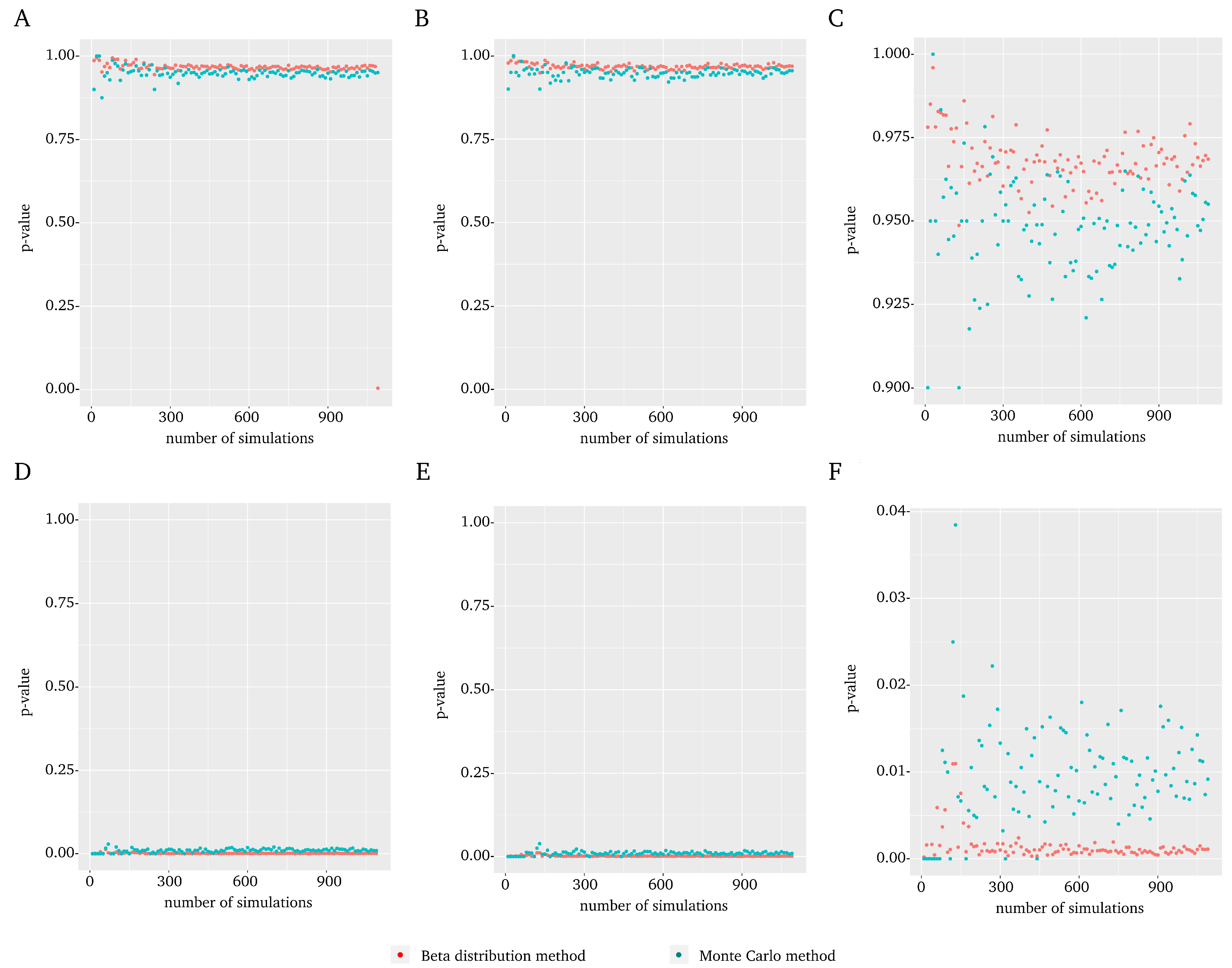
A representative example of the results is included in Figure 1 which shows the results of the MYC gene in experiment 1 (all results for each gene in each experiment are included in the Supplementary Material). In general, no differences were observed when using the t-Student distribution (Figure 1A) vs. normal (Figure 1B) distribution. On the other hand, major differences were found when the between-pair randomization (Figure 1A,B) was compared to complete randomization (Figure 1D,E). Regarding the number of simulations B (Figure 1C,F), the Montecarlo shows a greater variability than the beta distribution. Furthermore, it is not necessary to perform a large number of simulations to reach a value similar to the one obtained with the maximum evaluated. Indeed, from a small number of simulations and up, the value remains sufficiently stable.
From a statistical point of view the natural randomization distribution would be the between-pair randomization distribution because the original data in this example are paired. The statistical practice suggests that in such cases the between-pair distribution should provide a more powerful test. This is what it could be expected but surprisingly the observed p-values for complete distribution in our data seem to perform better. This particular gene is usually reported as associated with colorectal cancer. However, this is not a gold standard (in fact, there is none), but can be used to evaluate the method. The complete randomization distribution detects the gene, which does not happen with the between-pair randomization distribution. This and other examples suggested that we recommend the complete against the between-pair distribution independently of the original design.
Therefore, the parameters selected to be used in further experiments with the beta distribution method were the use of a normal distribution for the transformation between raw p-values and integrated p-values or score, the use of complete randomization and a number of simulations.
3.2. Simulation Study
A simulation study is proposed to evaluate the ability of the method to mark properly the significance of a gene. Artificial data coming from a model that mimics a real experiment will be generated but obviously the true significance of each fictitious gene is known. This is done with the following steps:
- A value for the false discovery rate (FDR) is given.
- For a given model, a realisation is generated.
- The Montecarlo p-value, our proposed score and the p-value of the moderated t-test are calculated. A number of simulations (from 100 to 1000) is used for the evaluation of the Montecarlo p-value and of the proposed score.
- The Benjamini–Hochberg correction will be applied to the three quantities evaluated in step 3.
- The features (genes) declared as significant will be compared with the (real) significant features.
- Steps 2 to 5 are repeated.
This experimental setup requires the generation of random but plausible matrices of expression. In order to do so two different stochastic models have been implemented and used. The first one has 200 significant genes and 800 non-significant genes. The expressions of a non-significant gene are independent samples from a normal distribution with mean 20 and standard deviation 1 (), whereas the expressions of a significant gene will come from a normal, too, , as in the first condition but with mean for a given positive . We will vary the value of from to 4 in steps of . Additionally the same number of observations are generated per condition. This sample size goes from 10 to 20 with unit increment. The number of replicas goes from 100 to 1000 with an increment of 100. Finally, different false discovery rates were used from to with an increment of .
The second stochastic model uses the gamma distribution instead of the normal distribution. The parameters were chosen in such a way that we reproduce the habitual setup, i.e., the expressions of a non-significant gene are independent samples from a gamma distribution with mean 20 and standard deviation 1, whereas the mean of the first group for significant features is equal to 20 and for the second group is (with taking values from to 4 in steps of ). The variance is equal to 1 for both groups. The false positive and false negative proportions were estimated (i.e., the type I and II errors).
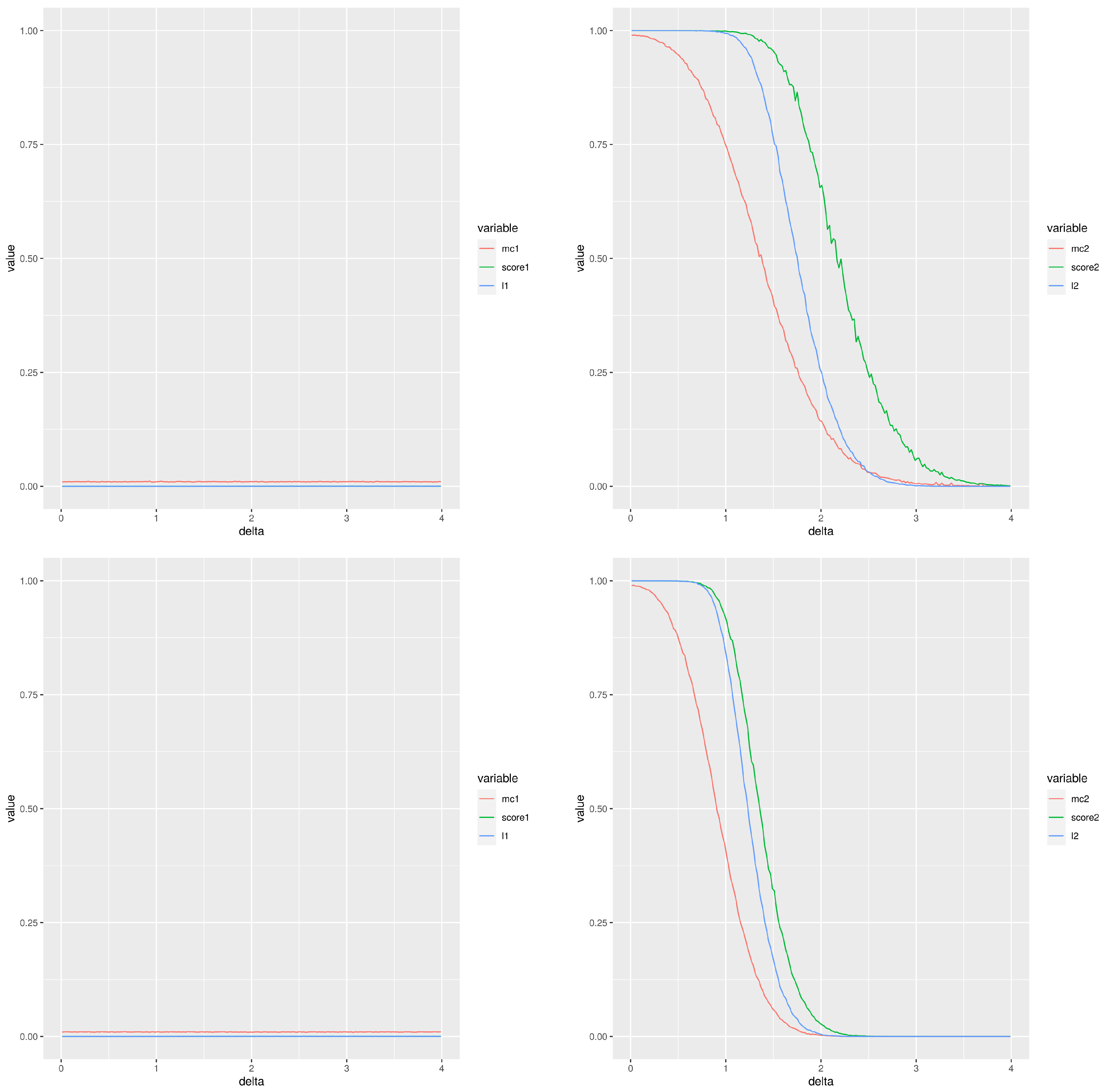
Figure 2 is an example of this simulation; it displays the two types of errors estimated for different experimental settings (the left column corresponds to type I error and the right column to type II error) using a total of 100 simulations and a normal cumulative distribution function. The two first rows correspond to , while the two last rows correspond to . The first and third rows correspond to a number of samples per group , whereas the second and fourth are for . The red, green and blue lines correspond to the Montecarlo method, our score and the moderated t-test, respectively. From the point of view of type I error, the performance of our score is very similar to the moderated t-test with values smaller than the Montecarlo p-value. The behaviour for the type II error is not so clear. When the groups compared have 20 values and then practically there is no difference between the methods except that the Montecarlo performs better for small differences between the means. A similar comment applies for comparisons of groups of 10 values, although the observed differences are greater. The performance of our score and that of the moderated p-values are very close. When smaller groups with 10 values are used, the Montecarlo p-value shows a lower type II error. The differences are smaller for than for .
In summary, our score improves the performance of the Montecarlo p-value for the type I error and it shows a behaviour very close to that of the moderated the p-values. If the type II error is considered, then the Montecarlo p-value shows the best performance and then our score. Additional plots with comparable results are included in the file SupplementaryMaterialAddons.pdf as supplementary material, in particular some GIF animations showing the behaviour of both types of error are shown.
The functions rArrayNorm and rArrayGamma included in the associated R package OMICfpp2 were used to generate the random expression matrices. The file fun-BetaMontecarlo20 contains the function doReplication used in the simulation study and the whole code is included in the last section of SupplementaryMaterialMethods_BetaMonteCarlo.pdf.
3.3. Using the Score with Real Datasets
Colorectal cancer datasets from different platforms were used to test the biological effectiveness of the proposed approach.
3.3.1. Using the Score for Multi-Cohort Analysis
The biological results of 21 colorectal cancer (CRC) datasets (see Table 1) were analyzed. As stated before, a normal distribution, complete randomization and 300 realizations were used. A total of 18 genes were found to be significant (score < 0.05) in all the microarrays of gene expression experiments (see Table 2). With a less restrictive criterion (namely, admit a gene if it was present in most of the studies, and missing in no more than two), 197 genes were significant since not all platforms include the same genes. With respect to the genes of the first criterion, most of these 18 were reported associated to colorectal cancer in experimental studies (see Section 4).
3.3.2. Score vs. Moderated p-Value
The moderated t-test method included in [17], (limma) is the most used method for statistical analysis of microarray datasets. Only the genes PRKAR2B and B3GALT4 were reported as significant in the 21 experiments by using the limma model and these two genes were also reported by our score (Table 2). Thus, the results obtained for genes in the Table 2 in each experiment using both methods were contrasted (Figure 3). In general, a clear pattern is observed through the experiments and for each gene using the proposed score, whereas this does not happen in the p-value of the moderated t-test method.
3.3.3. Using the Score on Different Platforms
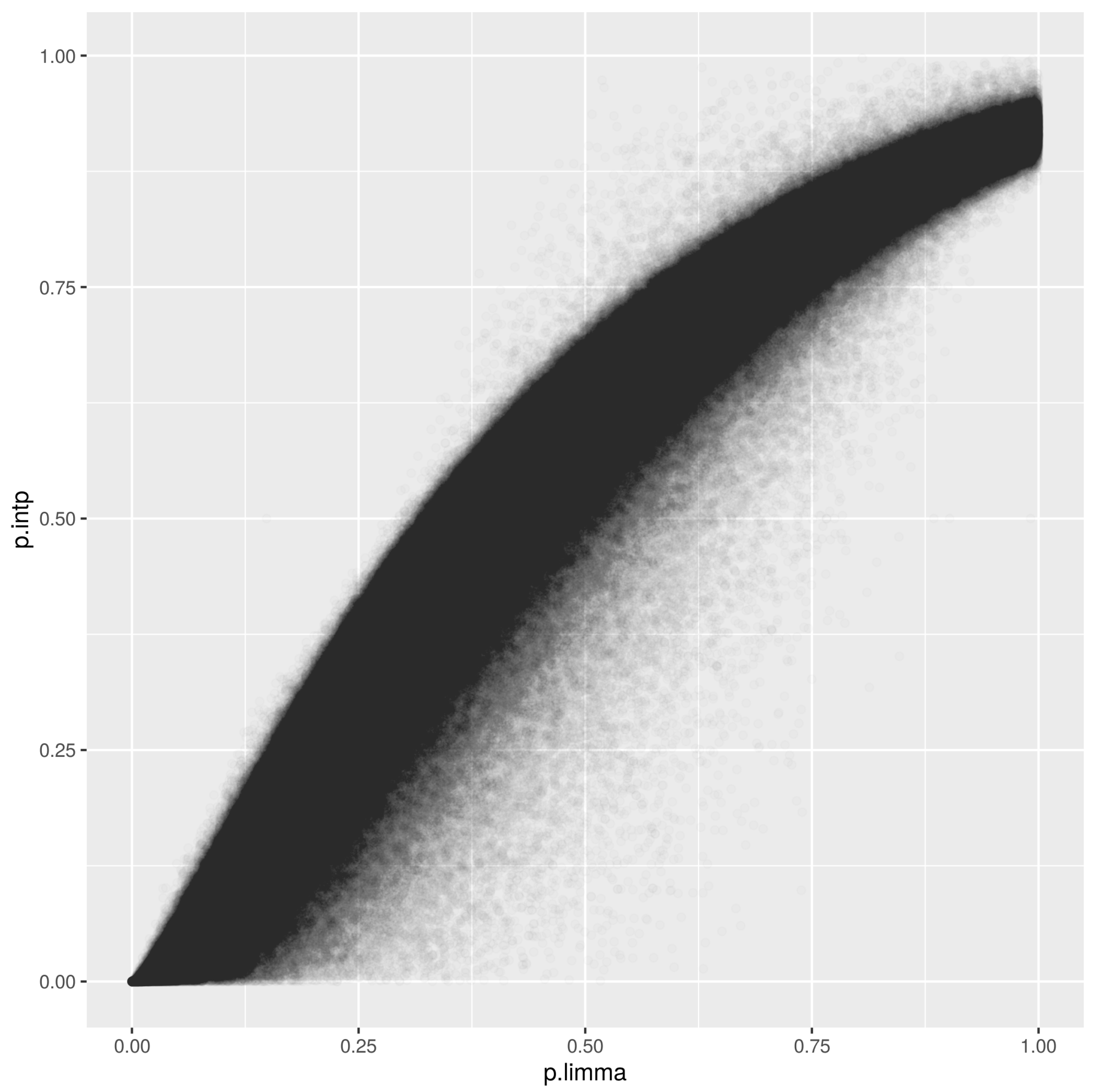
The infinium methylationEPIC array with 850,000 methylation sites throughout the human genome was analyzed using the score. The method proved to be efficient at analyzing the variables in a short period of time, without ties and with coherent biological results. Figure 4 displays our score versus the p-values using the well established method limma. The observed correlation is 0.96. Note that our approach does not need the parametric hypothesis.
Three RNA-Seq datasets were included in the analysis. The RNA-Seq data are counts. The top ten genes reported as differentially expressed in the PRJNA413956 experiment were ETFDH, RPSAP48, IPO7P2, CEMIP, LILRB5, KIFAP3, ENC1, LILRB5, TROAP and SMG9. For PRJNA218851 dataset were the genes OTOP3, BEST4, SPIB, HAUS6P3, UNC5C, OTOP2, CA7, SALL4, SH2D6 and ETV4. In both cases, the genes have previously been linked to CRC and other cancers, but new genes are also identified, which are reported to be associated with CRC here for the first time. Regarding the results obtained for the TCGA data, 3567 zeros were obtained, which does not allow order concerning the genes in this case. This also occurred with some of the microarray experiments, curiously, with larger sample sizes. To solve this problem, bootstrap were carried out, reducing the number of ties from 3567 to 195. More experiments are necessary to refine this option when the ties do not allow order concerning the significant genes.
4. Discussion
The major aim of the paper is to propose a score for ordering omics features (gene expression, methylation levels, etc.). It is proposed as an improvement of the usual Montecarlo p-value. It is closely related with it but improves the use of the randomization p-values. This is the focus of the paper. Both approaches have been compared with a well established methodology, the moderated t-test.
The expression data that come from microarrays and similar techniques have a high level of noise and masking between different effects. Therefore, comparisons between experiments performed in different although similar conditions might be biased which implies that the obtained p-values should be taken cautiously. Nevertheless, the relative importance of the expression of a gene in relation with the others in the same experiment is likely to be more meaningful, and therefore ordering is a key issue to be considered.
The central idea is to assume that p-values can be considered as samples that come from a beta distribution. We think that, given the flexibility of this family of distributions, the assumption is tenable. It is true that, if some knowledge of the underlying distribution of the given data were available, tailoring the distribution would be the obvious choice. However, in real situations the use of a beta distribution provides us a powerful tool. It is reasonable to wonder if the family of distributions covered by a beta family is flexible enough, i.e., if multimodal distributions could not be better fitted by something more complex like a mixture of beta distributions. Following the parsimony principle (use the simplest possible model that accounts for the data) we decided not to do so, since the results seem sensible. Nevertheless, this is a possibility to be explored in further work, taking into account the balance between goodness of fit and model complexity.
The raw statistics are transformed by a link function in order to obtain the p-values. These link functions are cumulative distribution functions. The score proposed is to be used mainly for ordering purposes. Nevertheless, the simulation study shows that if it is used as a p-value, the type I and type II errors are similar to those obtained with the moderated p-values, and both are different from the Montecarlo method. Notice that these results were obtained with fewer simulations i.e., less computational workload (with respect to the Montecarlo method) and without explicit assumptions about the specific distribution followed by the data (with respect to the moderated p-values method).
Moreover, the first step of the method used a t-test statistic, but it is worth mentioning that any other statistic could have been used, too. With respect to the practical application of the method, the cumulative distribution function used as a link does not seem to be crucial since similar results have been obtained using the distribution function of standard normal and of the t-Student distribution.
With respect to computation time, the method was programmed in C++ and automatically uses threads in several process units/cores if they are available, which makes it efficient, but it has been embedded into an R package to be called from R code, which makes it easier to use. The fact of being able to obtain good orderings with a relatively low number of randomizations constitutes an advantage with respect to the Montecarlo method.
Further, when paying attention to the generated ordering in a given experiment, our method is better than the classical Montecarlo method.
Finally, we proposed a pattern made of 18 genes that, using our approach, appear differentially expressed in the multi-cohort colorectal cancer datasets analysed. Most of these genes were found significant by validation in the relevant bibliography, for instance, PRKAR2B and B3GALT4 were found to be differentially expressed in all experiments, both using limma and our approach. The protein kinase cAMP-dependent type II regulatory subunit beta (PRKAR2B), has been associated with cancer [38], including colorectal cancer, in more than 50 publications. The B3GALT4 gene has been associated with the prognosis of colorectal cancer [39]. Other genes identified only by our score as the transforming growth factor beta induced (TGFBI) [40] or CXCL1 [41] are also widely related to cancer. Therefore, we consider it interesting to evaluate their joint biological function and their diagnostic value in subsequent studies, since the novel approach proposed here obtains reproducible results between experiments.
5. Conclusions
The approach proposed in this paper has shown a better performance than the Montecarlo p-values but with much fewer simulations and, differently to other methods, namely moderated t-test, without additional assumptions. It obtains reliable biological results in multiple platforms of omics data and across different experiments.
Supplementary Materials
The following are available online: The R package can be downloaded from https://johnford.uv.es/BetaMontecarlo/ (accessed on 5 June 2021). Also accessed on 5 June 2021 a copy of the following items, submitted as supplementaty material, too: Additional figures and GIF animations: https://johnford.uv.es/BetaMontecarlo/SupplementaryMaterialAddons.pdf; Supplementary Material Data (the preprocessing of the datasets used in the paper): https://johnford.uv.es/BetaMontecarlo/SupplementaryMaterialData.pdf; Supplementary Material Method (the code needed to reproduce the paper): https://johnford.uv.es/BetaMontecarlo/SupplementaryMaterialMethods.pdf; fun-BetaMontecarlo20.R (some functions used in the Supplementary Material Method file): https://johnford.uv.es/BetaMontecarlo/fun-BetaMonteCarlo20.R.
Author Contributions
Conceptualization and proofs, G.A.; methodology, G.A. and A.L.R.-C.; software, G.A. and J.D.; data curation, A.L.R.-C.; writing—original draft preparation, J.D.; biological problem formulation, A.L.R.-C. All authors have read and agreed to the published version of the manuscript.
Funding
This research was funded by the grants DPI2017-87333-R (G.A.) and the Chilean ANID/ FONDECYT-POSTDOCTORADO Nº3180486 (A.L.R.-C.).
Institutional Review Board Statement
Ethical review and approval were waived for this study, due to the fact that it uses publicly available data from previous studies which received its ethical approval when they were done.
Informed Consent Statement
Not applicable, since it was obtained when original studies that provide the publicly available data were done.
Conflicts of Interest
The authors declare no conflict of interest.
Appendix A
The following equations show in detail how to obtain the confidence interval mentioned in former sections.
Theorem A1.
The confidence interval for γ is given by
where is the quantile of the standard normal distribution.
Proof.
If we denote the density of the beta distribution as
then the log-likelihood for a single observation is given by
The first partial derivatives with respect to each variable are:
The second-order partial derivatives are:
The Fisher information matrix is . If we replace in it the unknown parameters and by those evaluated at we get the asymptotic covariance matrix for the Maximum Likelihood Estimator (MLE) that appears in the multivariate version of the delta method [12]. In fact, we have that
However, since we are really interested in the estimation of
for a given , we will apply the delta method using the scalar function h just defined obtaining
where . To apply this expression we need an estimator of . The partial derivatives are given by
but
and then
Note that where is the digamma function defined as
Finally, we have
Analogously
Then
and
As a last step, it will be needed to estimate the values of and . Note that we have the following Taylor series: and . If we denote the incomplete beta function then the above Taylor series can be applied leading to
Analogously
Therefore, the confidence interval for with a confidence level of will be
□
References
- Boulesteix, A.L.; Slawski, M. Stability and aggregation of ranked gene lists. Briefings Bioinform. 2009, 10, 556–568. [Google Scholar] [CrossRef] [PubMed] [Green Version]
- Chen, Q.; Zhou, X.J.; Sun, F. Finding Genetic Overlaps Among Diseases Based on Ranked Gene Lists. J. Comput. Biol. 2015, 22, 111–123. [Google Scholar] [CrossRef] [Green Version]
- Smyth, G.K.; Phipson, B. Permutation p-values Should Never Be Zero: Calculating Exact P-values When Permutations Are Randomly Drawn. Stat. Appl. Genet. Mol. Biol. 2010, 9, 39. [Google Scholar]
- Robert, C.; Casella, G. Introducing Monte Carlo Methods with R; Springer: New York, NY, USA, 2010. [Google Scholar] [CrossRef] [Green Version]
- Manly, B.F.J. Randomization, Bootstrap and Monte Carlo Methods in Biology, 3rd ed.; Texts in Statistical Science; Chapman & Hall/CRC: Boca Raton, FL, USA, 2007. [Google Scholar]
- Barnard, G. Contribution to the discussion of Professor Bartlett’s paper. J. R. Stat. Soc. B 1963, 25, 294. [Google Scholar]
- Bair, E. Identification of significant features in DNA microarray data. Wiley Interdiscip. Rev. Comput. Stat. 2013, 5, 309–325. [Google Scholar] [CrossRef]
- Hung, J.H.; Weng, Z. Analysis of Microarray and RNA-seq Expression Profiling Data. Cold Spring Harb. Protoc. 2017, 2017. [Google Scholar] [CrossRef] [PubMed]
- Halsey, L.G.; Curran-Everett, D.; Vowler, S.L.; Drummond, G.B. The fickle P value generates irreproducible results. Nat. Methods 2015, 12, 179–185. [Google Scholar] [CrossRef]
- Benjamin, D.J.; Berger, J.O.; Johannesson, M.; Nosek, B.A.; Wagenmakers, E.J.; Berk, R.; Bollen, K.A.; Brembs, B.; Brown, L.; Camerer, C.; et al. Redefine statistical significance. Nat. Hum. Behav. 2018, 2, 6–10. [Google Scholar] [CrossRef]
- Owen, C.E.B. Parameter Estimation for the Beta Distribution. Master’s Thesis, Department of Statistics, Brigham Young University, Provo, UT, USA, 2008. [Google Scholar]
- Agresti, A. Categorical Data Analysis, 3rd ed.; Wiley Series in Probability and Statistics; Wiley-Interscience: Hoboken, NJ, USA, 2013. [Google Scholar]
- Smyth, G.K. Linear Models and Empirical Bayes Methods for Assessing Differential Expression in Microarray Experiments. Stat. Appl. Genet. Mol. Biol. 2004, 3, 1–25. [Google Scholar] [CrossRef]
- Li, M.; Zhao, L.M.; Li, S.L.; Li, J.; Gao, B.; Wang, F.F.; Wang, S.P.; Hu, X.H.; Cao, J.; Wang, G.Y. Differentially expressed lncRNAs and mRNAs identified by NGS analysis in colorectal cancer patients. Cancer Med. 2018, 7, 4650–4664. [Google Scholar] [CrossRef] [Green Version]
- Kim, S.K.; Kim, S.Y.; Kim, J.H.; Roh, S.A.; Cho, D.H.; Kim, Y.S.; Kim, J.C. A nineteen gene-based risk score classifier predicts prognosis of colorectal cancer patients. Mol. Oncol. 2014, 8, 1653–1666. [Google Scholar] [CrossRef]
- Ishak, M.; Baharudin, R.; Mohamed Rose, I.; Sagap, I.; Mazlan, L.; Mohd Azman, Z.A.; Abu, N.; Jamal, R.; Lee, L.H.; Ab Mutalib, N.S. Genome-Wide Open Chromatin Methylome Profiles in Colorectal Cancer. Biomolecules 2020, 10, 719. [Google Scholar] [CrossRef]
- Smyth, G.; Ritchie, M.; Silver, J.; Wettenhall, J.; Thorne, N.; McCarthy, D.; Wu, D.; Hu, Y.; Shi, W.; Phipson, B.; et al. Limma: Linear Models for Microarray Data. R Package Version 3.22.7. 2015. Available online: https://rdrr.io/bioc/limma/ (accessed on 5 June 2021).
- Barrett, T.; Wilhite, S.E.; Ledoux, P.; Evangelista, C.; Kim, I.F.; Tomashevsky, M.; Marshall, K.A.; Phillippy, K.H.; Sherman, P.M.; Holko, M.; et al. NCBI GEO: Archive for functional genomics datasets—update. Nucleic Acids Res. 2012, 41, D991–D995. [Google Scholar] [CrossRef] [Green Version]
- Vlachavas, E.I.; Pilalis, E.; Papadodima, O.; Koczan, D.; Willis, S.; Klippel, S.; Cheng, C.; Pan, L.; Sachpekidis, C.; Pintzas, A.; et al. Radiogenomic Analysis of F-18-Fluorodeoxyglucose Positron Emission Tomography and Gene Expression Data Elucidates the Epidemiological Complexity of Colorectal Cancer Landscape. Comput. Struct. Biotechnol. J. 2019, 17, 177–185. [Google Scholar] [CrossRef]
- Galamb, O.; Spisák, S.; Sipos, F.; Tóth, K.; Solymosi, N.; Wichmann, B.; Krenács, T.; Valcz, G.; Tulassay, Z.; Molnár, B. Reversal of gene expression changes in the colorectal normal-adenoma pathway by NS398 selective COX2 inhibitor. Br. J. Cancer 2010, 102, 765–773. [Google Scholar] [CrossRef]
- Skrzypczak, M.; Goryca, K.; Rubel, T.; Paziewska, A.; Mikula, M.; Jarosz, D.; Pachlewski, J.; Oledzki, J.; Ostrowsk, J. Modeling oncogenic signaling in colon tumors by multidirectional analyses of microarray data directed for maximization of analytical reliability. PLoS ONE 2010, 5, e13091. [Google Scholar] [CrossRef]
- Tsukamoto, S.; Ishikawa, T.; Iida, S.; Ishiguro, M.; Mogushi, K.; Mizushima, H.; Uetake, H.; Tanaka, H.; Sugihara, K. Clinical significance of osteoprotegerin expression in human colorectal cancer. Clin. Cancer Res. 2011, 17, 2444–2450. [Google Scholar] [CrossRef] [PubMed] [Green Version]
- Uddin, S.; Ahmed, M.; Hussain, A.; Abubaker, J.; Al-Sanea, N.; AbdulJabbar, A.; Ashari, L.H.; Alhomoud, S.; Al-Dayel, F.; Jehan, Z.; et al. Genome-wide expression analysis of Middle Eastern colorectal cancer reveals FOXM1 as a novel target for cancer therapy. Am. J. Pathol. 2011, 178, 537–547. [Google Scholar] [CrossRef] [Green Version]
- Alhopuro, P.; Sammalkorpi, H.; Niittymäki, I.; Biström, M.; Raitila, A.; Saharinen, J.; Nousiainen, K.; Lehtonen, H.J.; Heliövaara, E.; Puhakka, J.; et al. Candidate driver genes in microsatellite-unstable colorectal cancer. Int. J. Cancer 2012, 130, 1558–1566. [Google Scholar] [CrossRef]
- Khamas, A.; Ishikawa, T.; Shimokawa, K.; Mogushi, K.; Iida, S.; Ishiguro, M.; Mizushima, H.; Tanaka, H.; Uetake, H.; Sugihara, K. Screening for epigenetically masked genes in colorectal cancer using 5-aza-2-deoxycytidine, microarray and gene expression profile. Cancer Genom. Proteom. 2012, 9, 67–75. [Google Scholar]
- Kemper, K.; Versloot, M.; Cameron, K.; Colak, S.; De Sousa, E.; Melo, F.; De Jong, J.H.; Bleackley, J.; Vermeulen, L.; Versteeg, R.; et al. Mutations in the Ras-Raf axis underlie the prognostic value of CD133 in colorectal cancer. Clin. Cancer Res. 2012, 18, 3132–3141. [Google Scholar] [CrossRef] [Green Version]
- Galamb, O.; Wichmann, B.; Sipos, F.; Spisák, S.; Krenács, T.; Tóth, K.; Leiszter, K.; Kalmár, A.; Tulassay, Z.; Molnár, B. Dysplasia-Carcinoma Transition Specific Transcripts in Colonic Biopsy Samples. PLoS ONE 2012, 7, e48547. [Google Scholar] [CrossRef] [PubMed]
- Martin, M.L.; Zeng, Z.; Adileh, M.; Jacobo, A.; Li, C.; Vakiani, E.; Hua, G.; Zhang, L.; Haimovitz-Friedman, A.; Fuks, Z.; et al. Logarithmic expansion of LGR5 + cells in human colorectal cancer. Cell. Signal. 2018, 42, 97–105. [Google Scholar] [CrossRef]
- Moreno, V.; Alonso, M.H.; Closa, A.; Vallés, X.; Diez-Villanueva, A.; Valle, L.; Castellví-Bel, S.; Sanz-Pamplona, R.; Lopez-Doriga, A.; Cordero, D.; et al. Colon-specific eQTL analysis to inform on functional SNPs. Br. J. Cancer 2018, 119, 971–977. [Google Scholar] [CrossRef] [Green Version]
- Ryan, B.M.; Zanetti, K.A.; Robles, A.I.; Schetter, A.J.; Goodman, J.; Hayes, R.B.; Huang, W.Y.; Gunter, M.J.; Yeager, M.; Burdette, L.; et al. Germline variation in NCF4, an innate immunity gene, is associated with an increased risk of colorectal cancer. Int. J. Cancer 2014, 134, 1399–1407. [Google Scholar] [CrossRef] [Green Version]
- Del Rio, M.; Mollevi, C.; Vezzio-Vie, N.; Bibeau, F.; Ychou, M.; Martineau, P. Specific Extracellular Matrix Remodeling Signature of Colon Hepatic Metastases. PLoS ONE 2013, 8, e74599. [Google Scholar] [CrossRef] [PubMed] [Green Version]
- Qu, X.; Sandmann, T.; Frierson, H.; Fu, L.; Fuentes, E.; Walter, K.; Okrah, K.; Rumpel, C.; Moskaluk, C.; Lu, S.; et al. Integrated genomic analysis of colorectal cancer progression reveals activation of EGFR through demethylation of the EREG promoter. Oncogene 2016, 35, 6403–6415. [Google Scholar] [CrossRef] [Green Version]
- Sabates-Bellver, J.; Van Der Flier, L.G.; De Palo, M.; Cattaneo, E.; Maake, C.; Rehrauer, H.; Laczko, E.; Kurowski, M.A.; Bujnicki, J.M.; Menigatti, M.; et al. Transcriptome profile of human colorectal adenomas. Mol. Cancer Res. 2007, 5, 1263–1275. [Google Scholar] [CrossRef] [PubMed] [Green Version]
- Hong, Y.; Downey, T.; Eu, K.W.; Koh, P.K.; Cheah, P.Y. A ’metastasis-prone’ signature for early-stage mismatch-repair proficient sporadic colorectal cancer patients and its implications for possible therapeutics. Clin. Exp. Metastasis 2010, 27, 83–90. [Google Scholar] [CrossRef]
- Abdueva, D.; Wing, M.; Schaub, B.; Triche, T.; Davicioni, E. Quantitative expression profiling in formalin-fixed paraffin-embedded samples by Affymetrix microarrays. J. Mol. Diagn. 2010, 12, 409–417. [Google Scholar] [CrossRef]
- Lin, G.; He, X.; Ji, H.; Shi, L.; Davis, R.W.; Zhong, S. Reproducibility Probability Score—Incorporating measurement variability across laboratories for gene selection. Nat. Biotechnol. 2006, 24, 1476–1477. [Google Scholar] [CrossRef] [PubMed]
- Matsuyama, T.; Ishikawa, T.; Mogushi, K.; Yoshida, T.; Iida, S.; Uetake, H.; Mizushima, H.; Tanaka, H.; Sugihara, K. MUC12 mRNA expression is an independent marker of prognosis in stage II and stage III colorectal cancer. Int. J. Cancer 2010, 127, 2292–2299. [Google Scholar] [CrossRef]
- Sha, J.; Han, Q.; Chi, C.; Zhu, Y.; Pan, J.; Dong, B.; Huang, Y.; Xia, W.; Xue, W. PRKAR2B promotes prostate cancer metastasis by activating Wnt/Beta-catenin and inducing epithelial-mesenchymal transition. J. Cell. Biochem. 2018, 119, 7319–7327. [Google Scholar] [CrossRef] [PubMed]
- Zhang, T.; Wang, F.; Wu, J.Y.; Qiu, Z.C.; Wang, Y.; Liu, F.; Ge, X.S.; Qi, X.W.; Mao, Y.; Hua, D. Clinical correlation of B7-H3 and B3GALT4 with the prognosis of colorectal cancer. World J. Gastroenterol. 2018, 24, 3538–3546. [Google Scholar] [CrossRef]
- Chiavarina, B.; Costanza, B.; Ronca, R.; Blomme, A.; Rezzola, S.; Chiodelli, P.; Giguelay, A.; Belthier, G.; Doumont, G.; Simaeys, G.V.; et al. Metastatic colorectal cancer cells maintain the TGFBeta program and use TGFBI to fuel angiogenesis. Theranostics 2021, 11, 1626–1640. [Google Scholar] [CrossRef]
- Zhuo, C.; Wu, X.; Li, J.; Hu, D.; Jian, J.; Chen, C.; Zheng, X.; Yang, C. Chemokine (C-X-C motif) ligand 1 is associated with tumor progression and poor prognosis in patients with colorectal cancer. Biosci. Rep. 2018, 38. [Google Scholar] [CrossRef] [Green Version]
Figure 1.
Comparison between the score and Montecarlo p-value using MYC gene results in the GSE110223 dataset as an example. For each plot, the Montecarlo p-value (blue) and the score (red) are displayed with respect to the number of randomizations. (A) Results obtained using the t-Student distribution and between-pair randomization. (B) Results obtained using normal distribution and between-pair randomization. (C) The plot shown in (B), using an enlarged scale to highlight the upper range. (D) Results obtained using t-Student distribution and complete randomization. (E) Results obtained using normal distribution and complete randomization. (F) The plot shown in (E), using an enlarged scale to highlight the lower range.

Figure 2.
Type I (left column) and type II (right column) errors when comparing two groups of gamma distributed random values. The difference between the means is the abscisa, . Please, notice the different scales in the Y-axis for types I and II. First and third rows (respectively, second and fourth rows) correspond to two groups of 10 values (respectively, 20 values). The two first rows (respectively, the two last rows) use a false discovery rate equal to (respectively, ).


Figure 3.
Comparison between common significant genes using the moderated p-value and our score. The 18 genes were reported with a score < 0.05 and with a moderated p-value . The cut off for score (A) and moderated t-test (B) are indicated by the vertical red dashed line in the density plot. All genes were represented across the 21 datasets with the corresponding score (C) and p-value (D).

Figure 4.
Comparison between our score and p-values obtained using the method limma for the infinium methylationEPIC array.
Figure 4.
Comparison between our score and p-values obtained using the method limma for the infinium methylationEPIC array.


Table 1.
Summary of datasets included in the analysis for testing the proposed method.
| Experiment | ID | Type | Platform | Samples |
|---|---|---|---|---|
| 1 | GSE110223 [19] | paired | hgu133a | 26 |
| 2 | GSE110224 [19] | paired | hgu133plus2 | 34 |
| 3 | GSE15960 [20] | paired | hgu133plus2 | 12 |
| 4 | GSE20916 [21] | non-paired | hgu133plus2 | 145 |
| 5 | GSE21510 [22] | non-paired | hgu133plus2 | 148 |
| 6 | GSE23878 [23] | non-paired | hgu133plus2 | 59 |
| 7 | GSE24514 [24] | non-paired | hgu133a | 49 |
| 8 | GSE32323 [25] | paired | hgu133plus2 | 34 |
| 9 | GSE33113 [26] | non-paired | hgu133plus2 | 96 |
| 10 | GSE37364 [27] | non-paired | hgu133plus2 | 52 |
| 11 | GSE41258 [28] | non-paired | hgu133a | 240 |
| 12 | GSE4183 [20] | non-paired | hgu133plus2 | 38 |
| 13 | GSE44076 [29] | paired | hgu219 | 196 |
| 14 | GSE44861 [30] | paired | hgu133a | 94 |
| 15 | GSE49355 [31] | non-paired | hgu133a | 38 |
| 16 | GSE77953 [32] | non-paired | hgu133a | 30 |
| 17 | GSE8671 [33] | paired | hgu133plus2 | 64 |
| 18 | GSE9348 [34] | non-paired | hgu133plus2 | 82 |
| 19 | GSE19249 [35] | non-paired | hgu133a2 | 23 |
| 21 | GSE41328 [36] | paired | hgu133plus2 | 10 |
| 23 | GSE18105 [37] | paired | hgu133plus2 | 34 |
| 24 | GSE149282 [16] | paired | Infinium MethylationEPIC | 24 |
| 25 | PRJNA413956 [14] | paired | Illumina HiSeq 3000 | 14 |
| 26 | PRJNA218851 [15] | paired | Illumina HiSeq 2000 | 36 |
| 27 | TCGA COAD | paired | RNA-Seq (not provided) | 100 |
Table 2.
The genes reported as significant in the 21 micro-array experiment analyzed using the beta distribution approach.
Table 2.
The genes reported as significant in the 21 micro-array experiment analyzed using the beta distribution approach.
| Symbol | Entrez ID | Min | Median | Max |
|---|---|---|---|---|
| TGFBI | 7045 | 0 | 0 | 0.0436 |
| BTNL3 | 10,917 | 0 | 4.74 | 0.0169 |
| RDH5 | 5959 | 0 | 9.99 | 0.0418 |
| XPOT | 11,260 | 0 | 2.66 | 0.0284 |
| ACADS | 35 | 0 | 3.62 | 0.0025 |
| GCG | 2641 | 0 | 1.40 | 0.0495 |
| CXCL1 | 2919 | 0 | 2.70 | 0.0492 |
| B3GALT4 | 8705 | 0 | 2.07 | 0.0333 |
| LRRFIP2 | 9209 | 0 | 3.47 | 0.0407 |
| CDHR5 | 53,841 | 0 | 4.28 | 0.0166 |
| HHLA2 | 11,148 | 0 | 2.28 | 0.0202 |
| PRKAR2B | 5577 | 0 | 3.10 | 0.0335 |
| HMGCL | 3155 | 0 | 2.09 | 0.0475 |
| FABP2 | 2169 | 0 | 6.20 | 0.0137 |
| STAP2 | 55,620 | 0 | 9.48 | 0.0419 |
| FXYD3 | 5349 | 0 | 9.48 | 0.0497 |
| ANO10 | 55,129 | 0 | 4.99 | 0.0199 |
| CKB | 1152 | 0 | 0.00024 | 0.0401 |
Publisher’s Note: MDPI stays neutral with regard to jurisdictional claims in published maps and institutional affiliations. |
© 2021 by the authors. Licensee MDPI, Basel, Switzerland. This article is an open access article distributed under the terms and conditions of the Creative Commons Attribution (CC BY) license (https://creativecommons.org/licenses/by/4.0/).
Share and Cite
MDPI and ACS Style
Riffo-Campos, A.L.; Ayala, G.; Domingo, J. Ordering of Omics Features Using Beta Distributions on Montecarlo p-Values. Mathematics 2021, 9, 1307. https://0-doi-org.brum.beds.ac.uk/10.3390/math9111307
AMA Style
Riffo-Campos AL, Ayala G, Domingo J. Ordering of Omics Features Using Beta Distributions on Montecarlo p-Values. Mathematics. 2021; 9(11):1307. https://0-doi-org.brum.beds.ac.uk/10.3390/math9111307
Chicago/Turabian StyleRiffo-Campos, Angela L., Guillermo Ayala, and Juan Domingo. 2021. "Ordering of Omics Features Using Beta Distributions on Montecarlo p-Values" Mathematics 9, no. 11: 1307. https://0-doi-org.brum.beds.ac.uk/10.3390/math9111307
Note that from the first issue of 2016, this journal uses article numbers instead of page numbers. See further details here.