
A Chaotic Krill Herd Optimization Algorithm for Global Numerical Estimation of the Attraction Domain for Nonlinear Systems


 , ,
, , 

Abstract
:1. Introduction
2. Estimation of the Domain of Attraction
2.1. Fundamentals of the Domain of Attraction
2.2. Concept Illustration for Enlarging the DA
2.2.1. Research on Maximum DA
2.2.2. Algorithm of Computing the DA
| Algorithm 1 DA estimation |
| Initialization: Initialize the parameters , , |
| Liniarization: The Jacobian of system (A1) at the origin and determine the matrix LF |
| for do |
| Evaluate , for each state |
| if && |
| else if && |
| If |
| end |
| end |
| end for |
| Result: Return the best value of DA |
| Draw the graphic Domain definite by ; |
| End. |
3. Proposed Krill Herd Algorithm for State Assessment
3.1. The Motivation for Using the Krill Herd Method
3.2. Krill Herd
- i.
- Krill movement due to other individuals;
- ii.
- Foraging behaviour;
- iii.
- Random diffusion;
3.2.1. Krill Movement Due to Other Individuals
3.2.2. Foraging Movement
3.2.3. Random Diffusion
3.3. Movement in KH
3.3.1. Crossover
3.3.2. Mutation
3.4. Computation of the Fitness Function
3.5. KH Computation Procedure
| Algorithm 2 The KH computional process |
| Begin |
| Initialization. Set the initial values for the population size (Np), the maximum induced speed (), the foraging speed (), the maximum diffusion speed ), the generation counter (m) and the maximum number of fitness function evaluations (). |
| Fitness evaluation. Evaluate the fitness function and randomly set up the position n x(i);i = 1,2,…,Np set of each krill individual then assess the fitness function value for all individuals. |
| Whilem < () or the stopping criteria are not accomplished do |
| Organize the population initiating from the best to worst. |
| Keep the best krill individual in “STORE” |
| fori = Np do |
| Compute the: a) Physical diffusion b) Foraging motion c) Induced motion |
| Implement genetic operators |
| Update the krill individual position in the search domain |
| Assess each krill individual based on its updated position |
| end for |
| Organize the population from best to worst and fix the current best one. Increment the counter m |
| m = m + 1 |
| end while |
| Results: Presentation of the results and visualition; |
| End. |
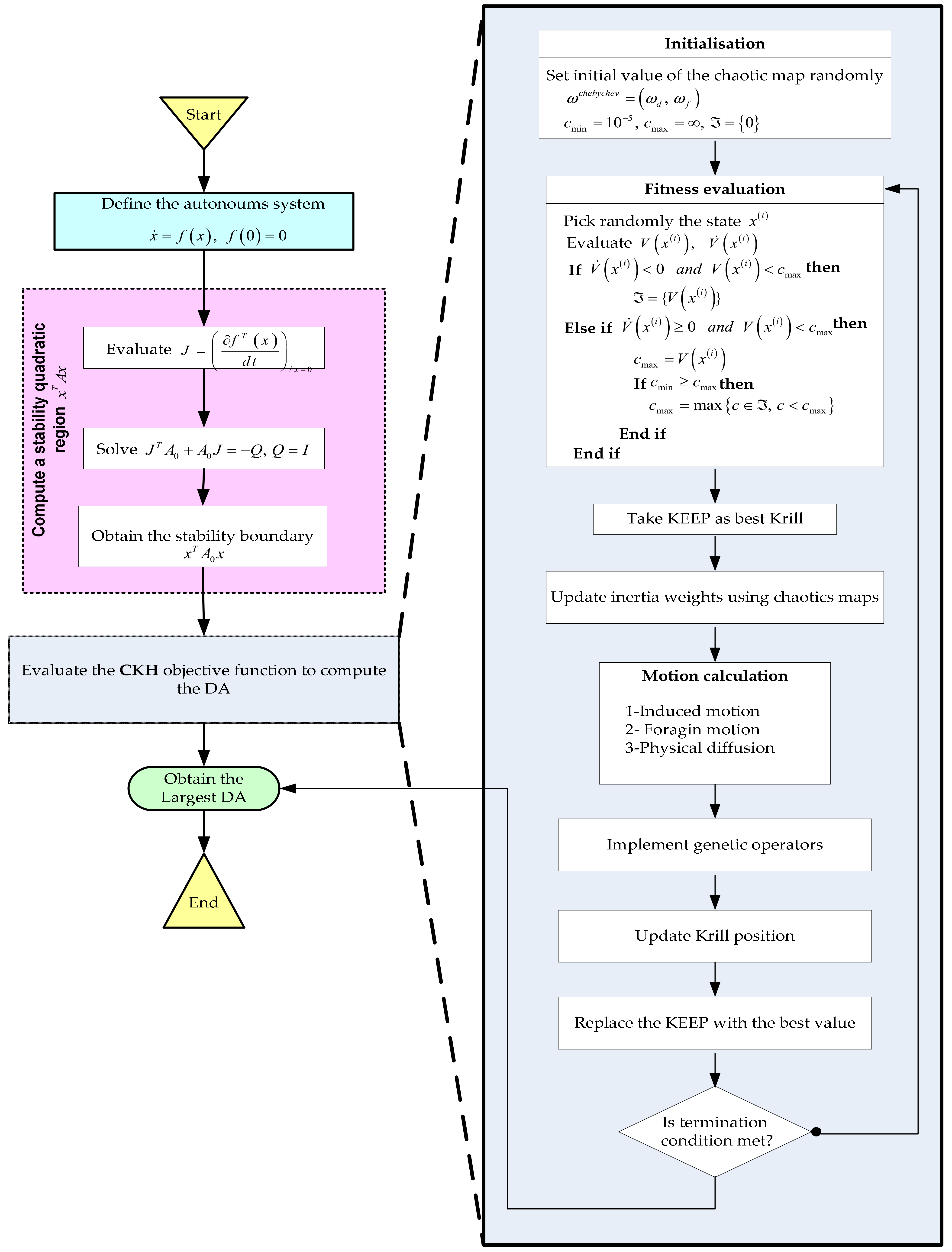
3.6. Fundamentals of Chaotic KH (CKH)
| Algorithm 3 The CKH computional process |
| Begin |
| Initialization. Initialize the CKH’s parameters m, (Np), (), (), () and () |
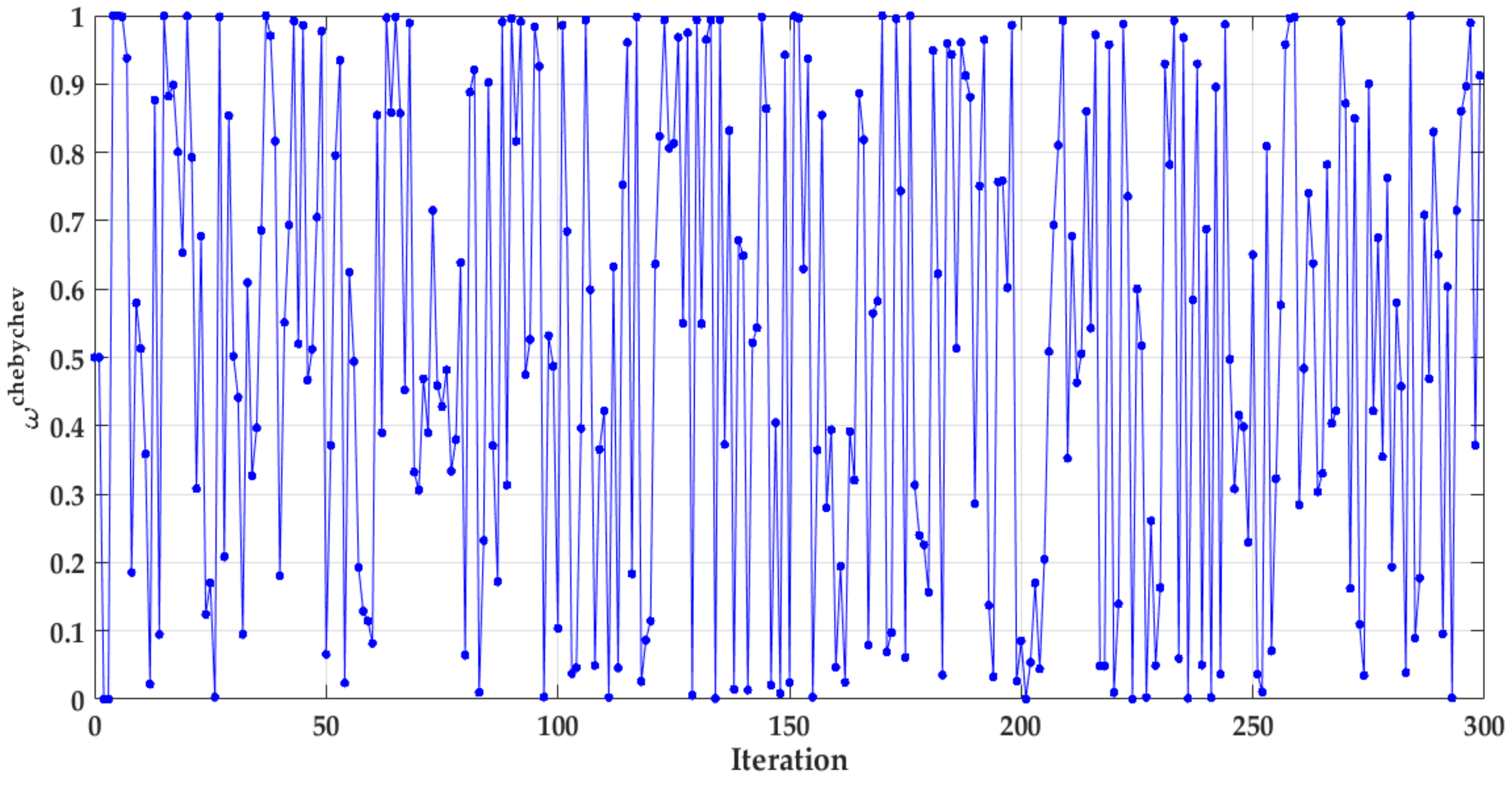
| Set up the chaotic maps value in random way and inertia weights ωchebychev = (ωd, ωf) as well. |
| STORE: number of the best krill swarm to retain from one generation to the next. |
| Fitness evaluation. Evaluate the fitness function and randomly set up the position x(i);i = 1,2,…,Np set of each krill individual, then assess the fitness function value for all individuals. |
| Whilem < or the stopping criteria are not accomplished do |
| Organize the population initiating from the best to worst. |
| Keep the best krill individual in “STORE” |
| for i = 1: Np do |
| Compute the: a) Physical diffusion b) Foraging motion c) Induced motion |
| Implement genetic operators |
| Update the krill individual position in the search domain |
| Assess each krill individual based on its updated position |
| end for |
| Update the “STORE” with the new best value; |
| Organize the population from best to worst and fix the current best one Increment the counter m: m = m + 1 |
| end while |
| Results: Presentation of the results and visualition; |
| End. |
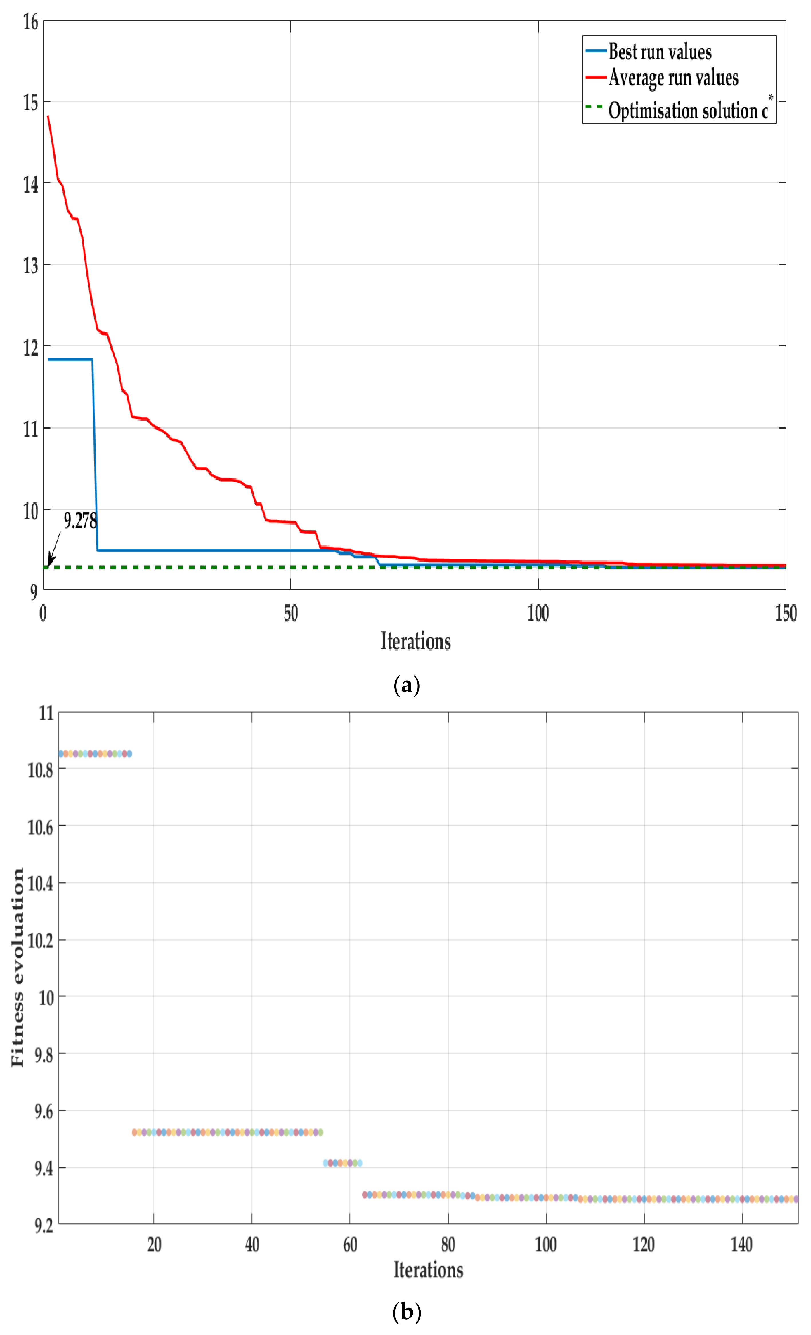
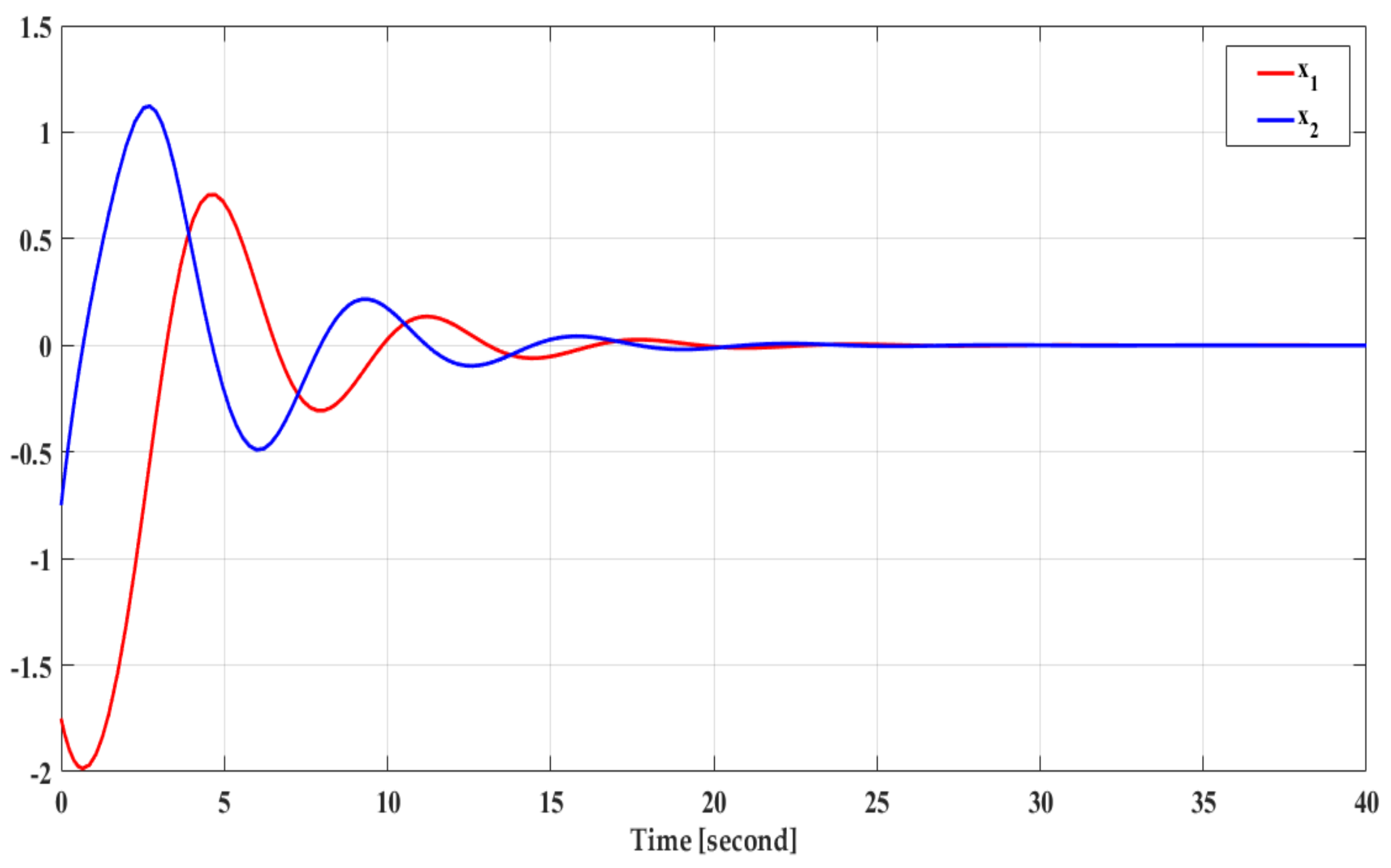
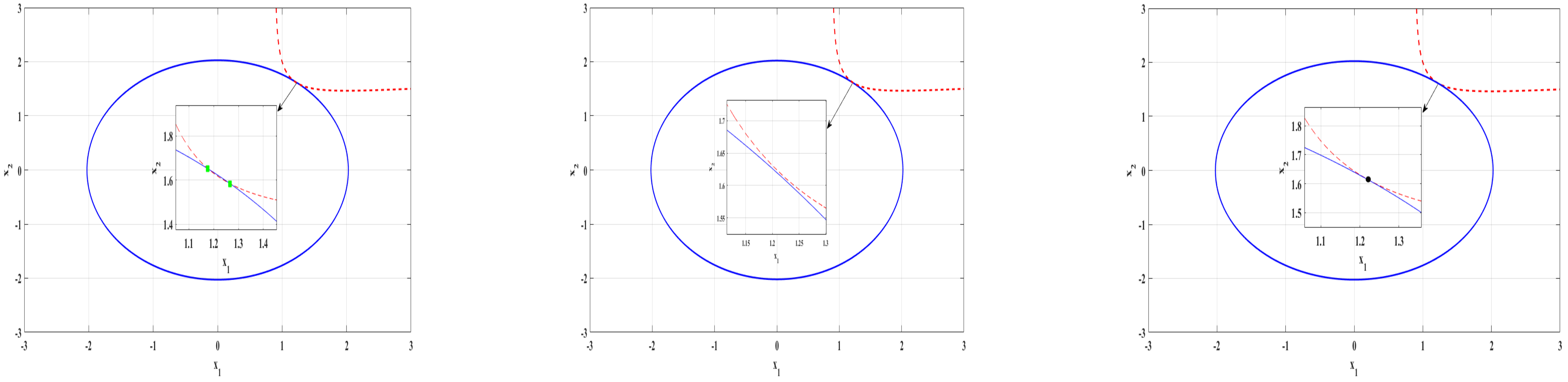
4. Illustrative Examples
4.1. Example 1
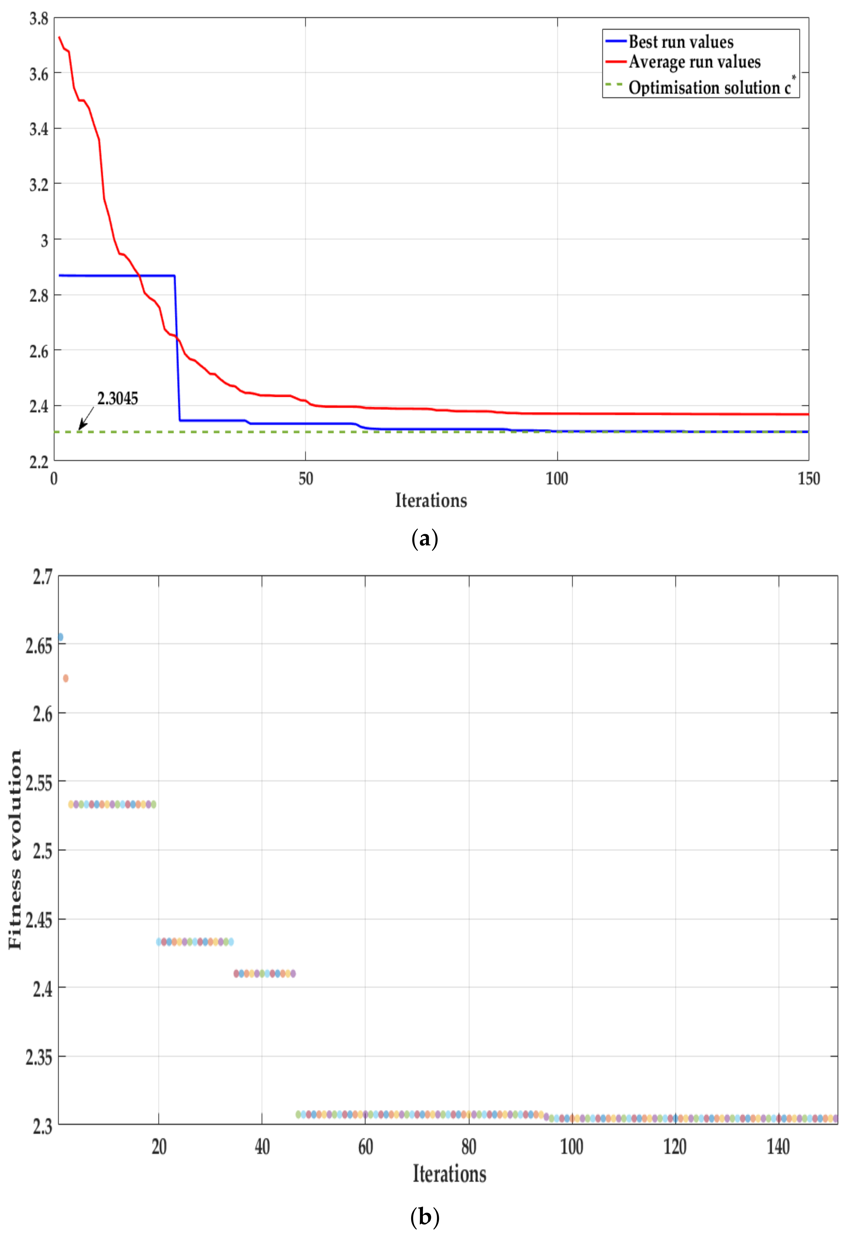
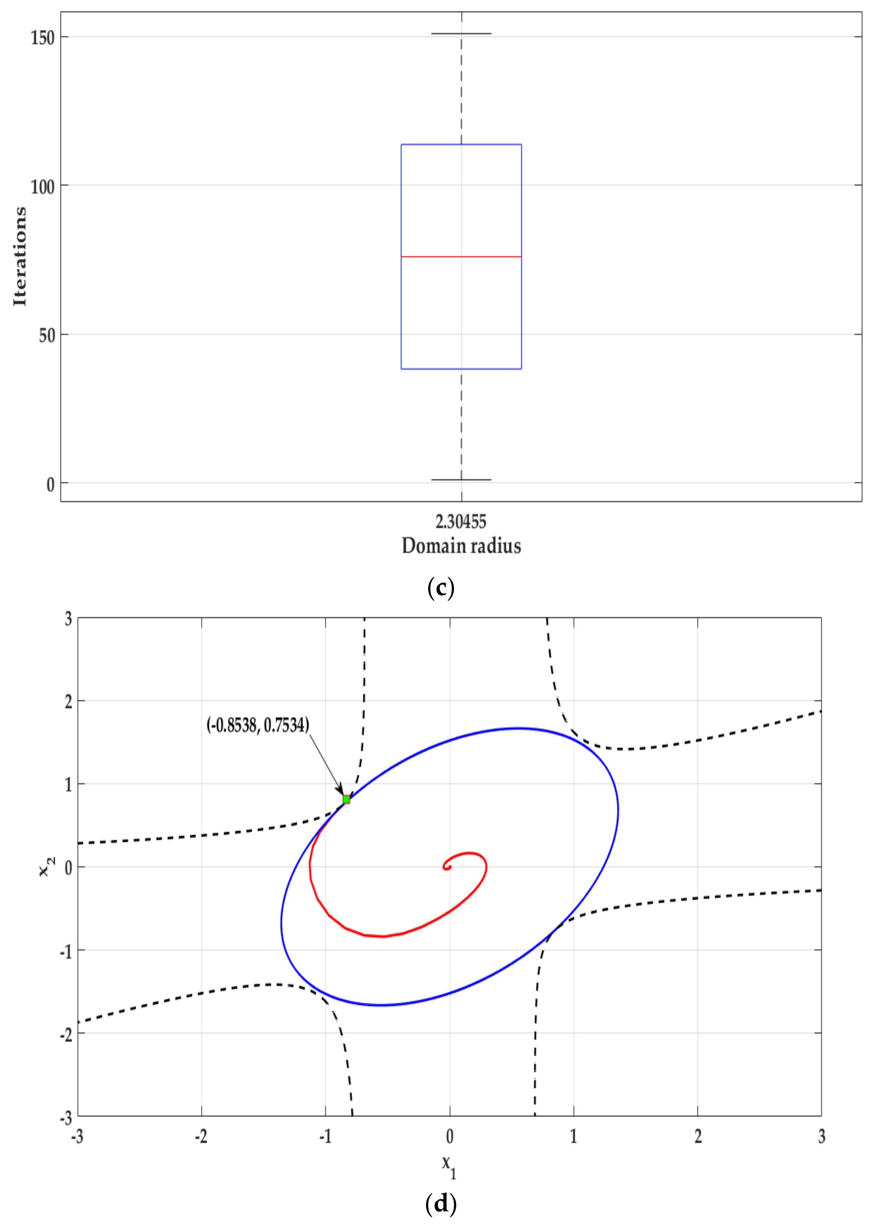
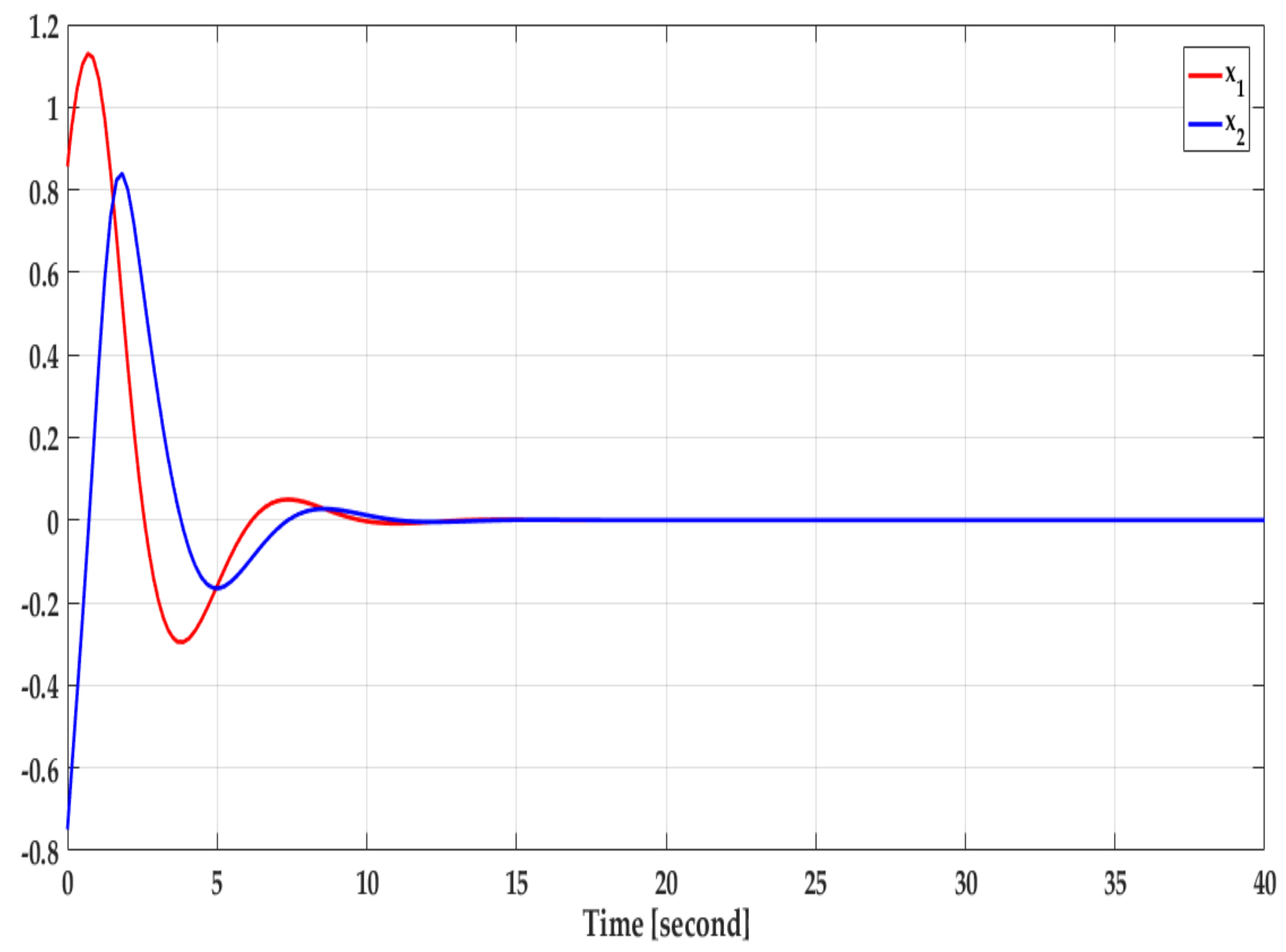
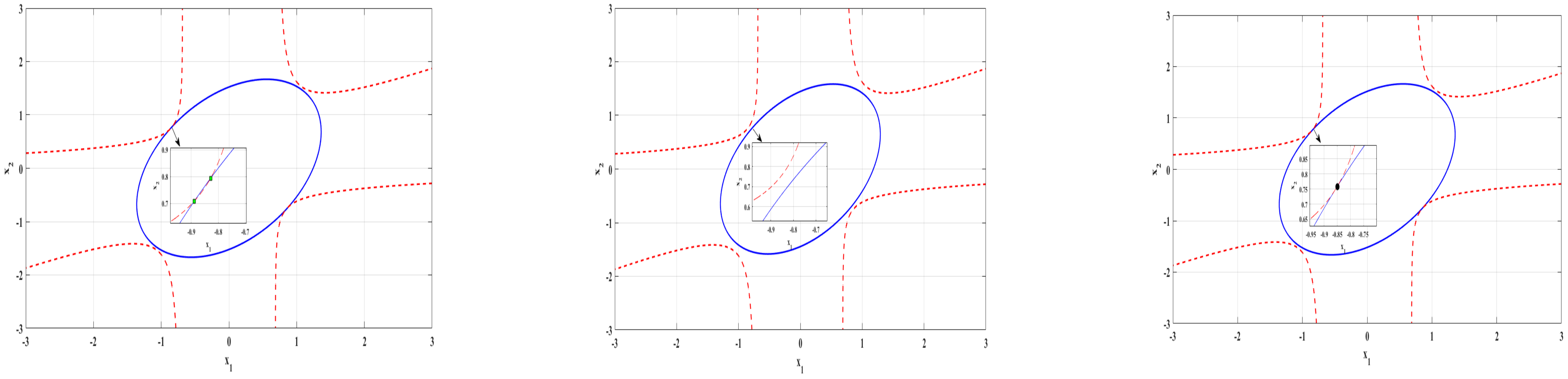
4.2. Example 2
5. Discussion
6. Conclusions
- The CKH technique suggested in the present study is straightforward, flexible, and easily understood. There are no challenges concerning the timing of parameter tuning; hence, it may be implemented for complex computational optimizations.
- The outcomes of the CKH algorithm, when benchmarked against the results of other popular optimization techniques, indicate the flexibility of the suggested approach.
- The proposed CKH technique requires less CPU time compared to other techniques because of the integration of chaos maps that provide chaotic maps benefits.
Author Contributions
Funding
Institutional Review Board Statement
Informed Consent Statement
Data Availability Statement
Conflicts of Interest
Appendix A. Theoretical Background, Fundamentals and Notations
- has a positive and definite value in D,
- Considering the trajectories of system (A1), the time derivative ofis semidefinite and negative inD.
References
- Díaz, D.; Valledor, P.; Ena, B.; Iglesias, M.; Menéndez, C. Improved Method for Parallelization of Evolutionary Metaheuristics. Mathematics 2020, 8, 1476. [Google Scholar] [CrossRef]
- Stefanoiu, D.; Borne, P.; Popescu, D.; Filip, F.G.; El Kamel, A. Metaheuristics—Local Methods. Optim. Eng. Sci. Approx. Metaheuristic Methods 2014, 1–52. [Google Scholar] [CrossRef]
- Kaveh, A.; Ghazaan, M.I. Meta-Heuristic Algorithms for Optimal Design of Real-Size Structures; Springer Science and Business Media LLC: Cham, Switzerland, 2018. [Google Scholar]
- Hamidi, F.; Jerbi, H.; Aggoune, W.; Djemai, M.; Abdkrim, M.N. Enlarging Region of Attraction Via LMI-Based Approach and Genetic Algorithm. In Proceedings of the 2011 International Conference on Communications, Computing and Control Applications (CCCA), Hammamet, Tunisia, 3–5 March 2011; pp. 1–6. [Google Scholar]
- Syafrudin, M.; Alfian, G.; Fitriyani, N.L.; Anshari, M.; Hadibarata, T.; Fatwanto, A.; Rhee, J. A Self-Care Prediction Model for Children with Disability Based on Genetic Algorithm and Extreme Gradient Boosting. Mathematics 2020, 8, 1590. [Google Scholar] [CrossRef]
- Ma, Z.; Yuan, X.; Han, S.; Sun, D. Improved Chaotic Particle Swarm Optimization Algorithm with More Symmetric Distribution for Numerical Function Optimization. Symmetry 2019, 11, 876. [Google Scholar] [CrossRef] [Green Version]
- Khan, S.; Kamran, M.; Rehman, O.U.; Liu, L.; Yang, S. A modified PSO algorithm with dynamic parameters for solving complex engineering design problem. Int. J. Comput. Math. 2017, 95, 2308–2329. [Google Scholar] [CrossRef]
- Jaber, A.S.; Abdulbari, H.A.; Shalash, N.A.; Abdalla, A.N. Garra Rufa-inspired optimization technique. Int. J. Intell. Syst. 2020, 35, 1831–1856. [Google Scholar] [CrossRef]
- Bansal, J.C.; Singh, P.K.; Pal, N.R. (Eds.) Evolutionary and Swarm Intelligence Algorithms; Springer: Cham, Switzerland, 2019. [Google Scholar]
- Tilahun, S.L.; Ngnotchouye, J.M.T. Firefly algorithm for discrete optimization problems: A survey. KSCE J. Civ. Eng. 2017, 21, 535–545. [Google Scholar] [CrossRef]
- Deng, W.; Xu, J.; Zhao, H. An Improved Ant Colony Optimization Algorithm Based on Hybrid Strategies for Scheduling Problem. IEEE Access 2019, 7, 20281–20292. [Google Scholar] [CrossRef]
- Wu, G.; Shen, X.; Li, H.; Chen, H.; Lin, A.; Suganthan, P. Ensemble of differential evolution variants. Inf. Sci. 2018, 423, 172–186. [Google Scholar] [CrossRef]
- Pradeepmon, T.G.; Panicker, V.V.; Sridharan, R. A heuristic algorithm enhanced with probability-based incremental learning and local search for dynamic facility layout problems. Int. J. Appl. Decis. Sci. 2018, 4, 352–389. [Google Scholar] [CrossRef]
- Prayogo, D.; Cheng, M.Y.; Wu, Y.W.; Herdany, A.A.; Prayogo, H. Differential Big Bang-Big Crunch algorithm for construction-engineering design optimization. Autom. Constr. 2018, 85, 290–304. [Google Scholar] [CrossRef]
- Mirjalili, S. Biogeography-Based Optimization. In Evolutionary Algorithms and Neural Networks; Springer: Cham, Switzerland, 2019; pp. 57–72. [Google Scholar]
- Ouyang, H.B.; Gao, L.Q.; Li, S.; Kong, X.Y.; Wang, Q.; Zou, D.X. Improved harmony search algorithm: LHS. Appl. Soft Comput. 2017, 53, 133–167. [Google Scholar] [CrossRef]
- Mareli, M.; Twala, B. An adaptive Cuckoo search algorithm for optimization. Appl. Comput. Inform. 2018, 2, 107–115. [Google Scholar] [CrossRef]
- Li, X.; Zhang, J.; Yin, M. Animal migration optimization: An optimization algorithm inspired by animal migration behavior. Neural Comput. Appl. 2014, 7, 1867–1877. [Google Scholar] [CrossRef]
- Singh, G.P.; Singh, A. Comparative study of krill herd, firefly and cuckoo search algorithms for unimodal and multimodal optimization. Int. J. Intell. Syst. Appl. Eng. 2014, 3, 26–37. [Google Scholar] [CrossRef]
- Cui, Z.; Li, F.; Zhang, W. Bat algorithm with principal component analysis. Int. J. Mach. Learn. Cybern. 2019, 3, 603–622. [Google Scholar] [CrossRef]
- Mishra, M.; Gunturi, V.R.; Maity, D. Teaching-learning-based optimization algorithm and its application in capturing critical slip surface in slope stability analysis. Soft Comput. 2020, 4, 2969–2982. [Google Scholar] [CrossRef]
- Talatahari, S.; Motamedi, P.; Azar, B.F.; Azizi, M. Tribe-charged system search for parameter configuration of nonlinear systems with large search domains. Eng. Optim. 2021, 53, 18–31. [Google Scholar] [CrossRef]
- Asteris, P.G.; Nozhati, S.; Nikoo, M.; Cavaleri, L.; Nikoo, M. Krill herd algorithm-based neural network in structural seismic reliability evaluation. Mech. Adv. Mater. Struct. 2018, 26, 1146–1153. [Google Scholar] [CrossRef]
- Wang, G.-G.; Gandomi, A.H.; Alavi, A.H.; Gong, D. A comprehensive review of krill herd algorithm: Variants, hybrids and applications. Artif. Intell. Rev. 2019, 51, 119–148. [Google Scholar] [CrossRef]
- Abualigah, L.; Khader, A.T.; Hanandeh, E.S. A combination of objective functions and hybrid Krill herd algorithm for text document clustering analysis. Eng. Appl. Artif. Intell. 2018, 73, 111–125. [Google Scholar] [CrossRef]
- Abualigah, L.M.; Khader, A.T.; Hanandeh, E.S.; Gandomi, A. A novel hybridization strategy for krill herd algorithm applied to clustering techniques. Appl. Soft Comput. 2017, 60, 423–435. [Google Scholar] [CrossRef]
- Wang, G.-G.; Guo, L.; Gandomi, A.; Hao, G.-S.; Wang, H. Chaotic Krill Herd algorithm. Inf. Sci. 2014, 274, 17–34. [Google Scholar] [CrossRef]
- Najafi, E.; Babuška, R.; Lopes, G.A. A fast sampling method for estimating the domain of attraction. Nonlinear Dyn. 2016, 2, 823–834. [Google Scholar] [CrossRef] [Green Version]
- Hachicho, O. A novel LMI-based optimization algorithm for the guaranteed estimation of the domain of attraction using rational Lyapunov functions. J. Frankl. Inst. 2007, 344, 535–552. [Google Scholar] [CrossRef]
- Khalil, H.K. Nonlinear Systems, 3rd ed.; Prentice Hall: Upper Saddle River, NJ, USA, 2002. [Google Scholar]
- Chesi, G. Rational Lyapunov functions for estimating and controlling the robust domain of attraction. Automatica 2013, 49, 1051–1057. [Google Scholar] [CrossRef] [Green Version]
- Jerbi, H.M.; Hamidi, F.; Ben Aoun, S.; Olteanu, S.C.; Popescu, D. Lyapunov-based Methods for Maximizing the Domain of Attraction. Int. J. Comput. Commun. Control. 2020, 15, 5. [Google Scholar] [CrossRef]
- Chesi, G. Computing Output Feedback Controllers to Enlarge the Domain of Attraction in Polynomial Systems. IEEE Trans. Autom. Control. 2004, 49, 1846–1850. [Google Scholar] [CrossRef]
- Ran, M.; Wang, Q.; Dong, C.; Ni, M. Multistage anti-windup design for linear systems with saturation nonlinearity: Enlargement of the domain of attraction. Nonlinear Dyn. 2015, 3, 1543–1555. [Google Scholar] [CrossRef]
- Hamidi, F.; Jerbi, H.; Aggoune, W.; Djemaï, M.; Abdelkrim, M.N. Enlarging the Domain of Attraction in Nonlinear Polynomial Systems. Int. J. Comput. Commun. Control. 2013, 8, 538. [Google Scholar] [CrossRef] [Green Version]
- Ermolin, V.S.; Vlasova, T.V. Identification of the Domain of Attraction. In Proceedings of the 2015 International Conference “Stability and Control Processes” in Memory of V.I. Zubov (SCP), Saint Petersburg, Russia, 5–9 October 2015; pp. 9–12. [Google Scholar]
- Doban, A.I.; Lazar, M. Computation of Lyapunov functions for nonlinear differential equations via a Massera-type construction. IEEE Trans. Autom. Control. 2017, 5, 1259–1272. [Google Scholar] [CrossRef] [Green Version]
- Chesi, G. Domain of Attraction: Estimates for Non-Polynomial Systems Via LMIs. In Proceedings of the 16th IFAC World Congress, Prague, Czech Republic, 3–8 July 2005. [Google Scholar]
- Hamidi, F.; Jerbi, H. On the Estimation of a Maximal Lyapunov Function and Domain of Attraction Determination Via a Genetic Algorithm. In Proceedings of the 2009 6th International Multi-Conference on Systems, Signals and Devices, Djerba, Tunisia, 23–26 March 2009; pp. 1–6. [Google Scholar]
- Zheng, X.; She, Z.; Lu, J.; Li, M. Computing multiple Lyapunov-like functions for inner estimates of domains of attraction of switched hybrid systems. Int. J. Robust Nonlinear Control. 2018, 17, 5191–5212. [Google Scholar] [CrossRef]
- Hamidi, F.; Jerbi, H.; Olteanu, S.C.; Popescu, D. An Enhanced Stabilizing Strategy for Switched Nonlinear Systems. Stud. Inform. Control. 2019, 28, 391–400. [Google Scholar] [CrossRef]
- Chesi, G.; Colaneri, P. Homogeneous rational Lyapunov functions for performance analysis of switched systems with arbitrary switching and dwell time constraints. IEEE Trans. Autom. Control. 2017, 10, 5124–5137. [Google Scholar] [CrossRef] [Green Version]
- Jerbi, H.; Braiek, N.B.; Bacha, A.B.B. A method of estimating the domain of attraction for nonlinear discrete-time systems. Arab. J. Sci. Eng. 2014, 5, 3841–3849. [Google Scholar] [CrossRef]
- Chesi, G.; Garulli, A.; Tesi, A.; Vicino, A. LMI-based computation of optimal quadratic Lyapunov functions for odd polynomial systems. Int. J. Robust Nonlinear Control. 2004, 15, 35–49. [Google Scholar] [CrossRef]
- Pitarch, J.L.; Sala, A.; Arino, C.V. Closed-Form Estimates of the Domain of Attraction for Nonlinear Systems via Fuzzy-Polynomial Models. IEEE Trans. Cybern. 2013, 44, 526–538. [Google Scholar] [CrossRef] [PubMed] [Green Version]
- Luk, C.K.; Chesi, G. On the estimation of the domain of attraction for discrete-time switched and hybrid nonlinear systems. Int. J. Syst. Sci. 2015, 15, 2781–2787. [Google Scholar] [CrossRef]
- Hamidi, F.; Aloui, M.; Jerbi, H.; Kchaou, M.; Abbassi, R.; Popescu, D.; Ben Aoun, S.; Dimon, C. Chaotic Particle Swarm Optimisation for Enlarging the Domain of Attraction of Polynomial Nonlinear Systems. Electronics 2020, 9, 1704. [Google Scholar] [CrossRef]
- Zečević, A.I.; Šiljak, D.D. Estimating the region of attraction for large-scale systems with uncertainties. Automatica 2010, 46, 445–451. [Google Scholar] [CrossRef]
- Topcu, U.; Packard, A.K.; Seiler, P.; Balas, G.J. Robust Region-of-Attraction Estimation. IEEE Trans. Autom. Control. 2009, 55, 137–142. [Google Scholar] [CrossRef] [Green Version]
- Swiatlak, R.; Tibken, B.; Paradowski, T.; Dehnert, R. An Interval Arithmetic Approach for the Estimation of the Robust Domain of Attraction for Nonlinear Autonomous Systems with Nonlinear Uncertainties. In Proceedings of the 2015 American Control Conference (ACC), Chicago, IL, USA, 1–3 July 2015; pp. 2679–2684. [Google Scholar]
- Nersesov, S.G.; Ashrafiuon, H.; Ghorbanian, P. On estimation of the domain of attraction for sliding mode control of underactuated nonlinear systems. Int. J. Robust Nonlinear Control. 2014, 5, 811–824. [Google Scholar] [CrossRef]
- Majumdar, A.; Vasudevan, R.; Tobenkin, M.; Tedrake, R. Convex Optimization of Nonlinear Feedback Controllers via Occupation Measures. Int. J. Robot. Res. 2014, 9, 1209–1230. [Google Scholar] [CrossRef]
- Jerbi, H. Estimations of the Domains of Attraction for Classes of Nonlinear Continuous Polynomial Systems. Arab. J. Sci. Eng. 2017, 42, 2829–2837. [Google Scholar] [CrossRef]
- Jemai, W.J.; Jerbi, H.; Abdelkrim, M.N. Nonlinear state feedback design for continuous polynomial systems. Int. J. Control. Autom. Syst. 2011, 9, 566–573. [Google Scholar] [CrossRef]
- Baier, R.; Gerdts, M. A Computational Method for Non-Convex Reachable Sets Using Optimal Control. In Proceedings of the 2009 European Control Conference (ECC), Budapest, Hungary, 23–26 August 2009; pp. 97–102. [Google Scholar]
- Bacanin, N.; Bezdan, T.; Tuba, E.; Strumberger, I.; Tuba, M. Monarch Butterfly Optimization Based Convolutional Neural Network Design. Mathematics 2020, 8, 936. [Google Scholar] [CrossRef]
- Baghban, A.; Jalali, A.; Shafiee, M.; Ahmadi, M.H.; Chau, K.-W. Developing an ANFIS-based swarm concept model for estimating the relative viscosity of nanofluids. Eng. Appl. Comput. Fluid Mech. 2019, 13, 26–39. [Google Scholar] [CrossRef] [Green Version]
- Matallana, L.G.; Blanco, A.M.; Bandoni, J.A. Estimation of domains of attraction: A global optimization approach. Math. Comput. Model. 2010, 52, 574–585. [Google Scholar] [CrossRef] [Green Version]


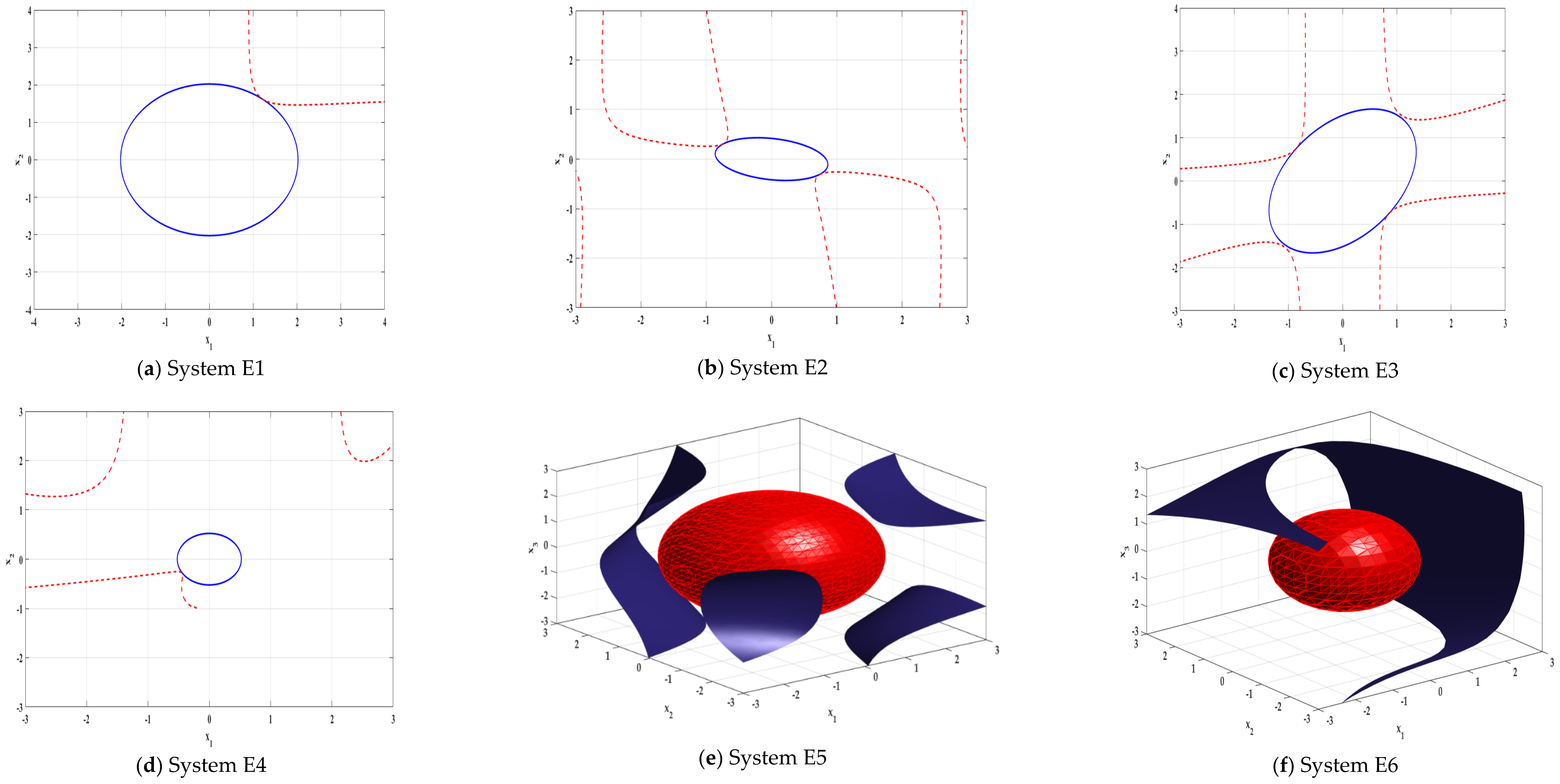
| Example | Systems Dynamics | Lyapunov Function | Estimated DA | Optimization Algorithm Convergence Time (ms) | Tangency Point (Best Solution) | ||||||
|---|---|---|---|---|---|---|---|---|---|---|---|
| [29] | [28] | CKH | [29] | [28] | CKH | [29] | [28] | CKH | |||
| E1 | 4.0804 | 4.112 | 4.0955 | - | 6.6 | 0.350 | - | - | |||
| E2 | 2.09 | 2.318 | 2.3045 | - | 6.7 | 0.542 | - | - | |||
| E3 | 0.699 | 0.708 | 0.6993 | - | 7.2 | 0.236 | - | - | |||
| E4 | 0.2737 | 0.278 | 0.2737 | - | 8.3 | 0.258 | - | - | |||
| E5 | 4.9188 | 4.971 | 4.969 | - | 8.4 | 0.77 | - | - | |||
| E6 | 2.655 | 2.887 | 2.6617 | - | 8.6 | 0.813 | - | - | |||
| Method | Pros | Cons |
|---|---|---|
| CKH |
|
|
| Sampling technique |
|
|
| Analytical method |
|
|
Publisher’s Note: MDPI stays neutral with regard to jurisdictional claims in published maps and institutional affiliations. |
© 2021 by the authors. Licensee MDPI, Basel, Switzerland. This article is an open access article distributed under the terms and conditions of the Creative Commons Attribution (CC BY) license (https://creativecommons.org/licenses/by/4.0/).
Share and Cite
Aloui, M.; Hamidi, F.; Jerbi, H.; Omri, M.; Popescu, D.; Abbassi, R. A Chaotic Krill Herd Optimization Algorithm for Global Numerical Estimation of the Attraction Domain for Nonlinear Systems. Mathematics 2021, 9, 1743. https://0-doi-org.brum.beds.ac.uk/10.3390/math9151743
Aloui M, Hamidi F, Jerbi H, Omri M, Popescu D, Abbassi R. A Chaotic Krill Herd Optimization Algorithm for Global Numerical Estimation of the Attraction Domain for Nonlinear Systems. Mathematics. 2021; 9(15):1743. https://0-doi-org.brum.beds.ac.uk/10.3390/math9151743
Chicago/Turabian StyleAloui, Messaoud, Faiçal Hamidi, Houssem Jerbi, Mohamed Omri, Dumitru Popescu, and Rabeh Abbassi. 2021. "A Chaotic Krill Herd Optimization Algorithm for Global Numerical Estimation of the Attraction Domain for Nonlinear Systems" Mathematics 9, no. 15: 1743. https://0-doi-org.brum.beds.ac.uk/10.3390/math9151743