An Extension of Explicit Coupling for Fluid–Structure Interaction Problems

Abstract

We present an extension of a non-iterative, partitioned method previously designed and used to model the interaction between an incompressible, viscous fluid and a thick elastic structure. The original method is based on the Robin boundary conditions and it features easy implementation and unconditional stability. However, it is sub-optimally accurate in time, yielding only $\mathcal{O}(\Delta t^{\frac{1}{2}})$ rate of convergence. In this work, we propose an extension of the method designed to improve the sub-optimal accuracy. We analyze the stability properties of the proposed method, showing that the method is stable under certain conditions. The accuracy and stability of the method are computationally investigated, showing a significant improvement in the accuracy when compared to the original scheme, and excellent stability properties. Furthermore, since the method depends on a combination parameter used in the Robin boundary conditions, whose values are problem specific, we suggest and investigate formulas according to which this parameter can be determined.

1. Introduction

Fluid–structure interaction (FSI) problems arise in many applications, such as aeroelasticity, biomechanics and automotive engineering. In biomedical applications, FSI models have been widely used to describe the interaction between blood and arterial walls. Combining state-of-the-art numerical algorithms for FSI problems with non-invasive clinical measurement tools provides an innovative approach to medical diagnosis and surgical decision making for many cardiovascular diseases, such as aneurysms and atherosclerosis. As a result, there is an increasing demand for fast and efficient numerical algorithms to solve FSI problems arising from biomedical applications.

The interaction between an incompressible, viscous fluid and an elastic structure is characterized by highly non-linear coupling between two different physical processes. As a result, a comprehensive study of such problems is challenging [1]. Solution strategies for FSI problems can be classified as monolithic and partitioned schemes. In monolithic algorithms, the entire coupled problem is solved as one system of algebraic equations, treating the coupling conditions implicitly. However, they can be quite expensive in terms of the computational time and memory requirements. Furthermore, they require well-designed preconditioners [2,3,4] in blood flow applications. Alternatively, to obtain smaller and better conditioned sub-problems, and treat each physical process separately, partitioned algorithms have been used. The development of partitioned numerical methods for FSI problems has been extensively studied in the literature. However, stability issues often arise as a result of the coupling at the interface. Even when the partitioning is carefully designed, stable partitioned algorithms may also suffer from the sub-optimal time accuracy [5,6,7,8,9].

The design of non-iterative, partitioned methods is particularly challenging when the dimension of the solid domain is the same as the dimension of the fluid domain, i.e., when the structure is thick. Thin structures, which are described by a lower-dimensional model, can easily be used in the design of partitioned methods based on the Robin boundary conditions since their entire domain is a part of the fluid domain boundary, which has been exploited in [8,10,11,12]. In cases when the structure is thick, such approaches can not be directly extended because the structure domain exists outside of the fluid domain, which makes the design of stable, non-iterative partitioned algorithms especially challenging.

A review of recent developments of robust monolithic fluid–structure interaction solvers can be found in [13]. Partitioned methods for FSI problems can be classified as strongly coupled, if the fluid and structure sub-problems require sub-iterations at each time step, or loosely coupled, if no sub-iterations are needed. Strongly coupled methods have been studied in [14,15,16,17,18], where the coupling conditions are linearly combined to obtain the generalized Robin interface conditions, which are then used in the fluid and/or structure sub-problems. Strongly coupled fictitious-pressure and fictitious-mass algorithms have also been proposed in [19,20], where the added mass effect is accounted for by incorporating additional terms into governing equations. Algorithms based on the Nitsche’s penalty method have been proposed in [6,21], where a weakly consistent stabilization term was added to obtain stability. However, since the rate of convergence in time was sub-optimal, a few defect-correction sub-iterations were performed. A loosely coupled, partitioned algorithm based on the so-called added-mass partitioned Robin conditions was proposed in [22], which was shown to be stable under a condition on the time step that depends on the structural parameters. The method was extended to finite deformations, and the explicit fluid solver was replaced by a fractional-step implicit–explicit scheme in [23]. A generalized Robin–Neumann explicit coupling scheme based on an interface operator accounting for the solid inertial effects within the fluid has been proposed in [7]. The scheme has been analyzed on a linear FSI problem and shown to be stable under a time-step condition. Previously, we developed a partitioned method for FSI with a thick, viscoelastic structure based on the Lie operator splitting approach [24]. However, the assumption that the structure is viscoelastic was necessary in the derivation of the scheme, and the solid viscosity was solved implicitly with the fluid problem. The scheme was shown to be stable under a time-step condition in [8].

A partitioned, loosely coupled method for FSI problems between an incompressible, viscous fluid and a thick, elastic structure was presented in [25] and further used in [5,9,26]. In the proposed method, the fluid and structure sub-problems are each discretized using the backward Euler method and solved separately using Robin boundary conditions at the interface. The Robin boundary conditions are obtained by linearly combining the kinematic and dynamic coupling conditions, and as such they depend on the combination parameter, $\alpha$. Using energy estimates for both fixed and moving domain FSI problems, the method is proved to be unconditionally stable. However, the accuracy of the method is shown to be only $\mathcal{O}(\Delta t^{\frac{1}{2}})$ in time [5,9], compared to the expected accuracy of $\mathcal{O}(\Delta t)$. The sub-optimal accuracy comes from the estimation of the terms present in the Robin coupling conditions. However, despite the sub-optimal accuracy, the method is attractive due to its unconditional stability, easy implementation and the fact that no sub-iterations are required between the fluid and solid sub-problems.

In this work, we propose an extension of the method used in [5,9,25,26], designed to restore the optimal rate of convergence. In particular, we consider an FSI problem where the fluid is modeled using the Navier–Stokes equations for an incompressible, viscous fluid, and the structure using the equations of linear elasticity. The Navier–Stokes equations are written in the arbitrary Lagrangian–Eulerian (ALE) [27,28,29] formulation to resolve the issues related to the deformation of the fluid mesh. We propose an alternative formulation of the Robin interface conditions, where a second-order extrapolation is used to achieve a better accuracy. The method is analyzed on a linear FSI problem, and shown to be stable under certain assumptions. The scheme is discretized in space using the finite element method and implemented to computationally study its stability and accuracy properties. Our simulations show a significant improvement in the accuracy, both in terms of the rates of convergence and the magnitude of the errors, when the new Robin boundary conditions are used. Our results also indicate that the theoretical stability conditions are not required to hold in order to achieve numerical stability. In the second example, we propose and investigate different formulas for computing the values of the combination parameter, $\alpha$, used in the Robin boundary conditions, providing guidance on how to determine the value of this parameter in the numerical simulations.

The outline of this paper is as follows: We define the problem in Section 2. In Section 3, we present the numerical methods and perform the stability analysis. Numerical examples are presented in Section 4. Section 5 highlights the conclusions of the main results presented in this paper.

2. Problem Description

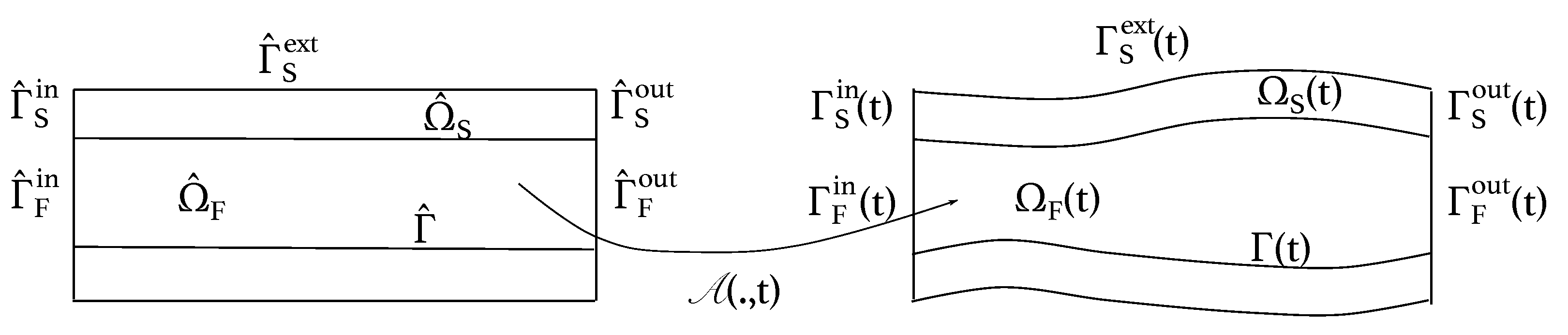
  Let ${\widehat{\Omega }}_F$ denote the reference fluid domain and ${\widehat{\Omega }}_S$ denote the reference structure domain. We assume that ${\widehat{\Omega }}_F,{\widehat{\Omega }}_S\subset {\mathbb{R}}^d,d=2,3$ are open, smooth sets of the same dimension, with common interface $\widehat{\Gamma }$. The fluid and structure domains at time t are denoted by ${\Omega }_F\left(t\right)$ and ${\Omega }_S\left(t\right)$, respectively. An example of a fluid–structure interaction problem is shown in Figure 1.

To track the deformation of the fluid domain in time, we introduce a smooth, invertible, ALE mapping $\mathcal{A}:{\widehat{\Omega }}_F\times [0,T]\to {\Omega }_F\left(t\right)$ given by

$$\mathcal{A}(\mathit{X},t)=\mathit{X}+{\mathit{\eta }}_F(\mathit{X},t),\mathrm{for}\mathrm{all} \mathit{X}\in {\widehat{\Omega }}_F,t\in [0,T],$$

where ${\mathit{\eta }}_F$ denotes the displacement of the fluid domain. We assume that ${\mathit{\eta }}_F$ equals the structure displacement on $\widehat{\Gamma }$, and is arbitrarily extended into the fluid domain ${\widehat{\Omega }}_F$ [30]. The fluid domain is determined by ${\Omega }_F\left(t\right)=\mathcal{A}({\widehat{\Omega }}_F,t).$ The deformation gradient of the fluid domain is denoted by $\mathit{F}=\nabla \mathcal{A},$ and its determinant by J.

We model the structure deformation in the Lagrangian framework, with respect to the reference domain ${\widehat{\Omega }}_S$. The fluid equations are described in the ALE formulation. To simplify the notation, we will write

$${\int }_{\Omega \left(t^m\right)}{\mathit{v}}^n\mathrm{instead}\mathrm{of}{\int }_{\Omega \left(t^m\right)}{\mathit{v}}^n\circ \mathcal{A}\left(t^n\right)\circ {\mathcal{A}}^{-1}\left(t^m\right)$$

whenever we need to integrate ${\mathit{v}}^n$ on a domain $\Omega \left(t^m\right)$, for $m\ne n$.

To model the fluid flow, we use the Navier–Stokes equations in the ALE formulation [24,30,31], given by

$$\begin{array}{ccc}\hfill & {\rho }_F\left({\partial }_t{\mathit{u}|}_{{\widehat{\Omega }}_F}+(\mathit{u}-\mathit{w})·\nabla \mathit{u}\right)=\nabla ·{\sigma }_F(\mathit{u},p)+{\mathit{f}}_F\hfill & \hfill \mathrm{in}{\Omega }_F\left(t\right)\times (0,T),\end{array}$$

(1)

$$\begin{array}{ccc}\hfill & \nabla ·\mathit{u}=0\hfill & \hfill \mathrm{in}{\Omega }_F\left(t\right)\times (0,T),\end{array}$$

(2)

where $\mathit{u}$ is the fluid velocity, ${\rho }_F$ is fluid density, ${\sigma }_F$ is the Cauchy stress tensor and ${\mathit{f}}_F$ is the forcing term. For a Newtonian fluid, the Cauchy stress tensor is given by ${\sigma }_F(\mathit{u},p)=-p\mathit{I}+2{\mu }_F\mathit{D}\left(\mathit{u}\right),$ where p is the fluid pressure, ${\mu }_F$ is the fluid viscosity and $\mathit{D}\left(\mathit{u}\right)=(\nabla \mathit{u}+{(\nabla \mathit{u})}^T)/2$ is the strain rate tensor. The domain velocity is denoted by $\mathit{w}={\partial }_t{\mathit{x}|}_{{\widehat{\Omega }}_F}={\partial }_t\mathcal{A}\circ {\mathcal{A}}^{-1}$ and ${\partial }_t{\mathit{u}|}_{{\widehat{\Omega }}_F}$ denotes the Eulerian description of the ALE field ${\partial }_t\mathit{u}\circ \mathcal{A}$ [32], i.e.,

$${\partial }_t{\mathit{u}(\mathit{x},t)|}_{{\widehat{\Omega }}_F}={\partial }_t\mathit{u}({\mathcal{A}}^{-1}(\mathit{x},t),t).$$

At the fluid external boundaries we prescribe the following boundary conditions:

$$\begin{array}{ccc}\hfill & \mathit{u}={\mathit{u}}_D\hfill & \hfill \mathrm{on}{\Gamma }_F^D\left(t\right)\times (0,T),\end{array}$$

(3)

$$\begin{array}{ccc}\hfill & {\sigma }_F{\mathit{n}}_F={\mathit{g}}_F\hfill & \hfill \mathrm{on}{\Gamma }_F^N\left(t\right)\times (0,T),\end{array}$$

(4)

where $\partial {\Omega }_F\left(t\right)=\Gamma \left(t\right)\cup {\Gamma }_F^D\left(t\right)\cup {\Gamma }_F^N\left(t\right)$, ${\mathit{n}}_F$ is the outward normal to the fluid domain, and ${\mathit{u}}_D$ and ${\mathit{g}}_F$ are given functions.

To describe the deformation of the structure, we use the linear elastodynamics equations written in the first order form as

$$\begin{array}{ccc}\hfill & {\rho }_S{\partial }_t\xi =\nabla ·{\sigma }_S+{\mathit{f}}_S\hfill & \hfill \mathrm{in}{\widehat{\Omega }}_S\times (0,T),\end{array}$$

(5)

$$\begin{array}{ccc}\hfill & {\partial }_t\mathit{\eta }=\xi \hfill & \hfill \mathrm{in}{\widehat{\Omega }}_S\times (0,T),\end{array}$$

(6)

where $\mathit{\eta }$ is the structure displacement, $\xi$ is the structure velocity, ${\rho }_S$ is the structure density, ${\mathit{f}}_S$ is the forcing term and ${\sigma }_S$ is the solid Cauchy stress tensor, given by

$$\begin{array}{c}\hfill {\sigma }_S\left(\mathit{\eta }\right)=2{\mu }_S\mathit{D}\left(\mathit{\eta }\right)+{\lambda }_S(\nabla ·\mathit{\eta })\mathit{I},\end{array}$$

where ${\mu }_S$ and ${\lambda }_S$ are Lamé constants. We define a norm associated with the structure elastic energy as

$$\begin{array}{c}\hfill {\parallel \mathit{\eta }\parallel }_S^2=2{\mu }_S{\parallel \mathit{D}\left(\mathit{\eta }\right)\parallel }_{L^2\left({\Omega }_S\right)}^2+{\lambda }_S{\parallel \nabla ·\mathit{\eta }\parallel }_{L^2\left({\Omega }_S\right)}^2.\end{array}$$

We assume that the following conditions are prescribed on the structure external boundaries:

$$\begin{array}{ccc}\hfill & \mathit{\eta }={\mathit{\eta }}_D\hfill & \hfill \mathrm{on}{\widehat{\Gamma }}_S^D\times (0,T),\end{array}$$

(7)

$$\begin{array}{ccc}\hfill & {\sigma }_S{\mathit{n}}_S={\mathit{g}}_S\hfill & \hfill \mathrm{on}{\widehat{\Gamma }}_S^N\times (0,T),\end{array}$$

(8)

where $\partial {\widehat{\Omega }}_S=\widehat{\Gamma }\cup {\widehat{\Gamma }}_S^D\cup {\widehat{\Gamma }}_S^N$, ${\mathit{n}}_S$ is the outward normal to the structure domain, and ${\mathit{\eta }}_D$ and ${\mathit{g}}_S$ are given functions.

To couple the fluid and structure sub-problems, we prescribe the kinematic and dynamic coupling conditions [30,31], given as follows:

Kinematic (no-slip) coupling condition describes the continuity of velocity at the fluid–structure interface:

$$\mathit{u}(\mathit{X}+\mathit{\eta }(\mathit{X},t),t)=\xi (\mathit{X},t)\mathrm{on}\widehat{\Gamma }\times (0,T).$$

(9)

Dynamic coupling condition describes the continuity of stresses at the fluid–structure interface:

$$J{\sigma }_F{\mathit{F}}^{-T}{\mathit{n}}_F+{\sigma }_S{\mathit{n}}_S=0\mathrm{on}\widehat{\Gamma }\times (0,T).$$

(10)

Initially, the fluid and structure are assumed to be at rest, with zero displacement from the reference configuration:

$$\mathit{u}=0\mathrm{in}{\widehat{\Omega }}_F,\mathit{\eta }=0,\xi =0\mathrm{in}{\widehat{\Omega }}_S\mathrm{at}t=0.$$

3. Numerical Method

Let $\Delta t$ be the time step and $t^n=n\Delta t$ for $n=0,\dots ,N,$ where $T=\Delta tN$ is the final time. We denote by $v^n$ the approximation of a time-dependent function v at time level $t^n$ and define the discrete backward difference operator $d_t{v}^{n+1}$ as

$$d_t{v}^{n+1}=\frac{v^{n+1}-v^n}{\Delta t}.$$

To simplify the analysis, we will assume that the fluid domain is fixed and drop the hat notation. This is a common assumptions in the analysis of partitioned schemes for FSI problems [6,8,11,22]. The extension of the proposed algorithm to moving domains is presented in Section 3.2.

To solve the fluid–structure interaction problem described in Section 2, a non-iterative partitioned method was proposed in [9]. The method is based on the Robin boundary condition obtained by multiplying the kinematic condition (9) by a combination parameter, $\alpha >0$, and adding it to the dynamic coupling condition (10). With the assumption that the domain is fixed, the method is described in Algortihm 1. The moving domain version of the method can be found in [9].

Algorithm 1 Given ${\mathit{u}}^0$ in ${\Omega }_F$, and ${\mathit{\eta }}^0,{\xi }^0$ in ${\Omega }_S$, for all $n\ge 1$, compute the following steps:

Structure sub-problem: Find ${\mathit{\eta }}^{n+1}$ and ${\xi }^{n+1}=d_t{\mathit{\eta }}^{n+1}$ such that $$\begin{array}{ccc}\hfill & {\rho }_S{d}_t{\xi }^{n+1}=\nabla ·{\sigma }_S\left({\mathit{\eta }}^{n+1}\right)+{\mathit{f}}_S\left(t^{n+1}\right)\hfill & \hfill \mathrm{in}{\Omega }_S,\end{array}$$ (11) $$\begin{array}{ccc}\hfill & \alpha {\xi }^{n+1}+{\sigma }_S\left({\mathit{\eta }}^{n+1}\right){\mathit{n}}_S=\alpha {\mathit{u}}^n-{\sigma }_F({\mathit{u}}^n,p^n){\mathit{n}}_F\hfill & \hfill \mathrm{on}\Gamma .\end{array}$$ (12) $$\begin{array}{ccc}\hfill & {\mathit{\eta }}^{n+1}={\mathit{\eta }}_D\left(t^{n+1}\right)\hfill & \hfill \mathrm{on}{\widehat{\Gamma }}_S^D,\end{array}$$ (13) $$\begin{array}{ccc}\hfill & {\sigma }_S\left({\mathit{\eta }}^{n+1}\right){\mathit{n}}_S={\mathit{g}}_S\left(t^{n+1}\right)\hfill & \hfill \mathrm{on}{\widehat{\Gamma }}_S^N.\end{array}$$ (14) Fluid sub-problem: Find ${\mathit{v}}^{n+1}$ and $p^{n+1}$ such that $$\begin{array}{ccc}\hfill & {\rho }_F{d}_t{\mathit{u}}^{n+1}=\nabla ·{\sigma }_F({\mathit{u}}^{n+1},p^{n+1})+{\mathit{f}}_F\left(t^{n+1}\right)\hfill & \hfill \mathrm{in}{\Omega }_F,\end{array}$$ (15) $$\begin{array}{ccc}\hfill & \nabla ·{\mathit{u}}^{n+1}=0\hfill & \hfill \mathrm{in}{\Omega }_F,\end{array}$$ (16) $$\begin{array}{ccc}\hfill & \alpha {\mathit{u}}^{n+1}+{\sigma }_F({\mathit{u}}^{n+1},p^{n+1}){\mathit{n}}_F=\alpha {\xi }^{n+1}+{\sigma }_F({\mathit{u}}^n,p^n){\mathit{n}}_F\hfill & \hfill \mathrm{on}\Gamma ,\end{array}$$ (17) $$\begin{array}{ccc}\hfill & {\mathit{u}}^{n+1}={\mathit{u}}_D\left(t^{n+1}\right)\hfill & \hfill \mathrm{on}{\Gamma }_F^D,\end{array}$$ (18) $$\begin{array}{ccc}\hfill & {\sigma }_F({\mathit{u}}^{n+1},p^{n+1}){\mathit{n}}_F={\mathit{g}}_F\left(t^{n+1}\right)\hfill & \hfill \mathrm{on}{\Gamma }_F^N.\end{array}$$ (19)

Since the method described in Algorithm 1 was shown to be unconditionally stable without sub-iterating between the fluid and structure sub-problems, but only $\mathcal{O}(\Delta t^{\frac{1}{2}})$ accurate, we propose to modify the coupling conditions in order to recover the first-order accuracy in time. Hence, we denote the extrapolation of a function v by

$$\delta v^n=2v^n-v^{n-1}.$$

The extrapolation will be used in the Robin boundary conditions in order to improve the convergence rate. The proposed method is given in the following algorithm.

To solve the problem in time, we use the finite element method. We introduce the following conforming finite element spaces

$$\begin{array}{cc}\hfill & V_h^F\subset V^F=\{\mathit{v}\in {\left(H^1\left({\Omega }_F\right)\right)}^d|\mathit{v}=0\mathrm{on}{\Gamma }_F^D\},\hfill \\ \hfill & Q_h\subset Q=L^2\left({\Omega }_F\right),\hfill \\ \hfill & V_h^S\subset V^S=\{\mathit{\eta }\in {\left(H^1\left({\Omega }_S\right)\right)}^d|\mathit{\eta }=0\mathrm{on}{\Gamma }_S^D\},\hfill \end{array}$$

based on conforming triangulations in ${\Omega }_F,{\Omega }_S$ with maximum triangle diameter h. We will use polynomials of degree $k\le 1$ for the fluid velocity, $r\le 1$ for the structure velocity and displacement, and $l\ge 0$ for the pressure. We assume that $k-1\le l\le k$. Whenever the considered velocity/pressure pair fails to satisfy the standard inf-sup condition [33], we assume that the following pressure stabilization operator

$$\frac{\gamma h^2}{{\mu }_F}{\int }_{{\Omega }_F}\nabla p_h\nabla {\psi }_h,$$

where $\gamma >0$, is added to the weak formulation. We introduce the following bilinear forms

$$\begin{array}{cc}\hfill & a_S(\mathit{\eta },\mathit{\zeta })=2{\mu }_S{\int }_{{\Omega }_S}\mathit{D}\left(\mathit{\eta }\right):\mathit{D}\left(\mathit{\zeta }\right)+{\lambda }_S{\int }_{{\Omega }_S}(\nabla ·\mathit{\eta })(\nabla ·\mathit{\zeta }),\forall \mathit{\eta },\mathit{\zeta }\in V^S,\hfill \\ \hfill & a_F(\mathit{u},\mathit{\varphi })=2{\mu }_F{\int }_{{\Omega }_F}\mathit{D}\left(\mathit{u}\right):\mathit{D}\left(\mathit{\varphi }\right),\forall \mathit{u},\mathit{\varphi }\in V^F,\hfill \\ \hfill & b_F(\psi ,\mathit{u})={\int }_{{\Omega }_F\left(t\right)}\nabla ·\mathit{u}\psi ,\forall \mathit{u}\in V^F,\psi \in Q.\hfill \end{array}$$

The weak formulation of the fully discrete method described in Algorithm 2 is given as follows.

Algorithm 2 Given ${\mathit{u}}^0$ in ${\Omega }_F$, and ${\mathit{\eta }}^0,{\xi }^0$ in ${\Omega }_S$, we first need to compute $p^1,{\mathit{u}}^1$ in ${\Omega }_F$, and ${\mathit{\eta }}^1,{\xi }^1$ in ${\Omega }_S$. A monolithic method could be used. Then, for all $n\ge 2$, compute the following steps:

Structure sub-problem: Find ${\mathit{\eta }}^{n+1}$ and ${\xi }^{n+1}=d_t{\mathit{\eta }}^{n+1}$ such that $$\begin{array}{ccc}\hfill & {\rho }_S{d}_t{\xi }^{n+1}=\nabla ·{\sigma }_S\left({\mathit{\eta }}^{n+1}\right)+{\mathit{f}}_S\left(t^{n+1}\right)\hfill & \hfill \mathrm{in}{\Omega }_S,\end{array}$$ (20) $$\begin{array}{ccc}\hfill & \alpha {\xi }^{n+1}+{\sigma }_S\left({\mathit{\eta }}^{n+1}\right){\mathit{n}}_S=\alpha \delta {\mathit{u}}^n-{\sigma }_F(\delta {\mathit{u}}^n,\delta p^n){\mathit{n}}_F\hfill & \hfill \mathrm{on}\Gamma ,\end{array}$$ (21) $$\begin{array}{ccc}\hfill & {\mathit{\eta }}^{n+1}={\mathit{\eta }}_D\left(t^{n+1}\right)\hfill & \hfill \mathrm{on}{\widehat{\Gamma }}_S^D,\end{array}$$ (22) $$\begin{array}{ccc}\hfill & {\sigma }_S\left({\mathit{\eta }}^{n+1}\right){\mathit{n}}_S={\mathit{g}}_S\left(t^{n+1}\right)\hfill & \hfill \mathrm{on}{\widehat{\Gamma }}_S^N.\end{array}$$ (23) Fluid sub-problem: Find ${\mathit{u}}^{n+1}$ and $p^{n+1}$ such that $$\begin{array}{ccc}\hfill & {\rho }_F{d}_t{\mathit{u}}^{n+1}=\nabla ·{\sigma }_F({\mathit{u}}^{n+1},p^{n+1})+{\mathit{f}}_F\left(t^{n+1}\right)\hfill & \hfill \mathrm{in}{\Omega }_F,\end{array}$$ (24) $$\begin{array}{ccc}\hfill & \nabla ·{\mathit{u}}^{n+1}=0\hfill & \hfill \mathrm{in}{\Omega }_F,\end{array}$$ (25) $$\begin{array}{ccc}\hfill & \alpha {\mathit{u}}^{n+1}+{\sigma }_F({\mathit{u}}^{n+1},p^{n+1}){\mathit{n}}_F=\alpha {\xi }^{n+1}+{\sigma }_F(\delta {\mathit{u}}^n,\delta p^n){\mathit{n}}_F\hfill & \hfill \mathrm{on}\Gamma ,\end{array}$$ (26) $$\begin{array}{ccc}\hfill & {\mathit{u}}^{n+1}={\mathit{u}}_D\left(t^{n+1}\right)\hfill & \hfill \mathrm{on}{\Gamma }_F^D,\end{array}$$ (27) $$\begin{array}{ccc}\hfill & {\sigma }_F({\mathit{u}}^{n+1},p^{n+1}){\mathit{n}}_F={\mathit{g}}_F\left(t^{n+1}\right)\hfill & \hfill \mathrm{on}{\Gamma }_F^N.\end{array}$$ (28)

Structure sub-problem: Find ${\xi }_h^{n+1}$ and ${\mathit{\eta }}_h^{n+1}$, where ${\xi }_h^{n+1}=d_t{\mathit{\eta }}_h^{n+1}$, such that for all ${\mathit{\zeta }}_h\in V_h^S$ we have

$$\begin{array}{cc}\hfill & {\rho }_S{\int }_{{\Omega }_S}{d}_t{\xi }_h^{n+1}·{\mathit{\zeta }}_{h}d\mathit{x}+a_S({\mathit{\eta }}_h^{n+1},{\mathit{\zeta }}_h)+\alpha {\int }_{\Gamma }({\xi }_h^{n+1}-\delta {\mathit{u}}_h^n)·{\mathit{\zeta }}_{h}d\mathit{x}\hfill \\ \hfill & =-{\int }_{\Gamma }{\sigma }_F(\delta {\mathit{u}}^n,\delta p^n){\mathit{n}}_F·{\mathit{\zeta }}_{h}d\mathit{x}+{\int }_{{\Omega }_S}{\mathit{f}}_S\left(t^{n+1}\right)·{\xi }_h.\hfill \end{array}$$

(29)

Fluid sub-problem: Find ${\mathit{u}}_h^{n+1}$ and $p_h^{n+1}$ such that for all ${\mathit{\varphi }}_h\in V_h^F$ and ${\psi }_h\in Q_h$ we have

$$\begin{array}{cc}\hfill & {\rho }_F{\int }_{{\Omega }_F}{d}_t{\mathit{u}}_h^{n+1}·{\mathit{\varphi }}_{h}d\mathit{x}+a_F({\mathit{u}}_h^{n+1},{\mathit{\varphi }}_h)-b_F(p_h^{n+1},{\mathit{\varphi }}_h)+b_F({\psi }_h,{\mathit{u}}_h^{n+1})\hfill \\ \hfill & +\frac{\gamma h^2}{{\mu }_F}{\int }_{{\Omega }_F}\nabla p_h\nabla {\psi }_h+\alpha {\int }_{\Gamma }({\mathit{u}}_h^{n+1}-{\xi }_h^{n+1})·{\mathit{\varphi }}_{h}d\mathit{x}\hfill \\ \hfill & ={\int }_{\Gamma }{\sigma }_F(\delta {\mathit{u}}^n,\delta p^n){\mathit{n}}_F·{\mathit{\varphi }}_{h}d\mathit{x}.+{\int }_{{\Omega }_F}{\mathit{f}}_F\left(t^{n+1}\right)·{\mathit{\varphi }}_h.\hfill \end{array}$$

(30)

3.1. Stability Analysis

In this section, we prove the stability of the partitioned method presented in Algorithm 2. In the following, we will use the polarized identity given by

$$\begin{array}{c}\hfill 2(a-c)b=a^2-c^2-{(a-b)}^2+{(b-c)}^2\end{array}$$

(31)

Let ${\mathcal{E}}^n$ denote the sum of the kinetic and elastic energy of the solid, and kinetic energy of the fluid, defined as

$$\begin{array}{c}\hfill {\mathcal{E}}^n=\frac{{\rho }_S}{2}\parallel {\xi }_h^n{\parallel }_{L^2\left({\Omega }_S\right)}^2+\frac{1}{2}\parallel {\mathit{\eta }}_h^n{\parallel }_S^2+\frac{{\rho }_F}{2}{\parallel {\mathit{u}}_h^n\parallel }_{L^2\left({\Omega }_F\right)}^2,\end{array}$$

let ${\mathcal{D}}^n$ denote the fluid viscous dissipation, given by

$$\begin{array}{c}\hfill {\mathcal{D}}^n=\Delta t\sum _{k=1}^{n-1}{\parallel \mathit{D}\left({\mathit{u}}_h^{k+1}\right)\parallel }_{L^2\left({\Omega }_F\right)}^2,\end{array}$$

let ${\mathcal{N}}^n$ denote the terms present due to numerical dissipation

$$\begin{array}{cc}\hfill {\mathcal{N}}^n=& \frac{{\rho }_S\Delta t^2}{2}\sum _{k=1}^{n-1}{∥d_t{\xi }_h^{k+1}∥}_{L^2\left({\Omega }_S\right)}^2+\frac{\Delta t^2}{2}\sum _{k=1}^{n-1}{∥d_t{\mathit{\eta }}_h^{k+1}∥}_S^2+\frac{{\rho }_F\Delta t^2}{2}\sum _{k=1}^{n-1}{\parallel d_t{\mathit{u}}_h^{k+1}\parallel }_{L^2\left({\Omega }_F\right)}^2\hfill \\ \hfill & +\frac{\alpha \Delta t}{2}\sum _{k=1}^{n-1}\left(\parallel {\mathit{u}}_h^{k+1}{\parallel }_{L^2(\Gamma )}^2+{\parallel {\xi }_h^{k+1}-\delta {\mathit{u}}_h^k\parallel }_{L^2(\Gamma )}^2\right)+\frac{\Delta t}{2\alpha }\sum _{k=1}^{n-1}{\parallel {\sigma }_F({\mathit{u}}_h^{k+1},p_h^{k+1}){\mathit{n}}_F\parallel }_{L^2(\Gamma )}^2\hfill \end{array}$$

and let ${\mathcal{S}}^n$ denote the term due to the pressure stabilization

$$\begin{array}{cc}\hfill {\mathcal{S}}^n=& \Delta t\sum _{k=1}^{n-1}{\parallel \nabla p_h^{n+1}\parallel }_{L^2\left({\Omega }_F\right)}^2.\hfill \end{array}$$

The stability result is given in the following theorem.

Theorem 1.

Let ${\left\{({\xi }_h^n,{\mathit{\eta }}_h^n,{\mathit{u}}_h^n,p_h^n)\right\}}_{1\le n\le N}$ be the solution of (29) and (30). Assume that the system is isolated, i.e., ${\mathit{u}}_D={\mathit{\eta }}_D={\mathit{g}}_F={\mathit{g}}_S={\mathit{f}}_F={\mathit{f}}_S=0$. Furthermore, assume that

$$\begin{array}{c}{ϵ}_1:=2{\mu }_F-5\alpha C_T^2{C}_P{C}_K^2-\frac{40{\mu }_F^2{C}_{TI}{k}^2}{\alpha h}>0\mathrm{and}{ϵ}_2:=\frac{\gamma h^2}{{\mu }_F}-\frac{10C_T^2{C}_P}{\alpha }>0\end{array}$$

(32)

Then, the following estimate holds:

$$\begin{array}{cc}\hfill & {\mathcal{E}}^N+{ϵ}_1{\mathcal{D}}^N+{ϵ}_2{\mathcal{S}}^N\le {\mathcal{E}}^1+\frac{2C_T^2{C}_P\Delta t}{\alpha }\left(5\parallel \nabla p_h^1{\parallel }_{L^2\left({\Omega }_F\right)}^2+{\parallel \nabla p_h^0\parallel }_{L^2\left({\Omega }_F\right)}^2\right)\hfill \\ \hfill & +\left(\alpha \Delta t{C}_T^2{C}_P{C}_K^2+\frac{8{\mu }_F^2{C}_{TI}{k}^2\Delta t}{\alpha h}\right)(5\parallel \mathit{D}\left({\mathit{u}}_h^1\right){\parallel }_{L^2\left({\Omega }_F\right)}^2+\parallel \mathit{D}\left({\mathit{u}}_h^0\right){\parallel }_{L^2\left({\Omega }_F\right)}^2).\hfill \end{array}$$

Proof. 

We let ${\mathit{\zeta }}_h={\xi }_h^{n+1}$ in (29) and ${\mathit{\varphi }}_h={\mathit{u}}_h^{n+1},{\psi }_h=p_h^{n+1}$ in (30). Multiplying by $\Delta t$, using (31) and adding equations together, we obtain

$$\begin{array}{cc}\hfill & \frac{{\rho }_S}{2}\left(\parallel {\xi }_h^{n+1}{\parallel }_{L^2\left({\Omega }_S\right)}^2-{\parallel {\xi }_h^n\parallel }_{L^2\left({\Omega }_S\right)}^2\right)+\frac{{\rho }_S\Delta t^2}{2}{∥d_t{\xi }_h^{n+1}∥}_{L^2\left({\Omega }_S\right)}^2+\frac{1}{2}\left(\parallel {\mathit{\eta }}_h^{n+1}{\parallel }_S^2-{\parallel {\mathit{\eta }}_h^n\parallel }_S^2\right)\hfill \\ \hfill & +\frac{\Delta t^2}{2}{∥d_t{\mathit{\eta }}_h^{n+1}∥}_S^2+\frac{{\rho }_F}{2}\parallel {\mathit{u}}_h^{n+1}{\parallel }_{L^2\left({\Omega }_F\right)}^2-\frac{{\rho }_F}{2}\parallel {\mathit{u}}_h^n{\parallel }_{L^2\left({\Omega }_F\right)}^2+\frac{{\rho }_F\Delta t^2}{2}{\parallel d_t{\mathit{u}}_h^{n+1}\parallel }_{L^2\left({\Omega }_F\right)}^2\hfill \\ \hfill & +2{\mu }_F\Delta t\parallel \mathit{D}\left({\mathit{u}}_h^{n+1}\right){\parallel }_{L^2\left({\Omega }_F\right)}^2+\frac{\alpha \Delta t}{2}(\parallel {\mathit{u}}_h^{n+1}{\parallel }_{L^2(\Gamma )}^2-\parallel \delta {\mathit{u}}_h^n{\parallel }_{L^2(\Gamma )}^2)\hfill \\ \hfill & +\frac{\alpha \Delta t}{2}(\parallel {\xi }_h^{n+1}-\delta {\mathit{u}}_h^n{\parallel }_{L^2(\Gamma )}^2+\parallel {\mathit{u}}_h^{n+1}-{\xi }_h^{n+1}{\parallel }_{L^2(\Gamma )}^2)+\frac{\gamma \Delta x^2\Delta t}{{\mu }_F}{\parallel \nabla p_h^{n+1}\parallel }_{L^2\left({\Omega }_F\right)}^2\hfill \\ \hfill & =\Delta t{\int }_{\Gamma }{\sigma }_F(\delta {\mathit{u}}_h^n,\delta p_h^n){\mathit{n}}_F·\left({\mathit{u}}_h^{n+1}-{\xi }_h^{n+1}\right)d\mathit{x}.\hfill \end{array}$$

(33)

To estimate the integral on the right-hand side, we use (26) and (31) as follows

$$\begin{array}{cc}\hfill & \Delta t{\int }_{\Gamma }{\sigma }_F(\delta {\mathit{u}}_h^n,\delta p_h^n){\mathit{n}}_F·\left({\mathit{u}}_h^{n+1}-{\xi }_h^{n+1}\right)d\mathit{x}\hfill \\ \hfill & =\frac{\Delta t}{\alpha }{\int }_{\Gamma }{\sigma }_F(\delta {\mathit{u}}_h^n,\delta p_h^n){\mathit{n}}_F·\left({\sigma }_F(\delta {\mathit{u}}_h^n,\delta p_h^n){\mathit{n}}_F-{\sigma }_F({\mathit{u}}_h^{n+1},p_h^{n+1}){\mathit{n}}_F\right)d\mathit{x}\hfill \\ \hfill & =\frac{\Delta t}{2\alpha }\left(\parallel {\sigma }_F(\delta {\mathit{u}}_h^n,\delta p_h^n){\mathit{n}}_F{\parallel }_{L^2(\Gamma )}^2-{\parallel {\sigma }_F({\mathit{u}}_h^{n+1},p_h^{n+1}){\mathit{n}}_F\parallel }_{L^2(\Gamma )}^2\right)\hfill \\ \hfill & +\frac{\Delta t}{2\alpha }{\parallel {\sigma }_F(-{\mathit{u}}_h^{n+1}+\delta {\mathit{u}}_h^n,-p_h^{n+1}+\delta p_h^n){\mathit{n}}_F\parallel }_{L^2(\Gamma )}^2\hfill \end{array}$$

(34)

Using (26) again, we have

$$\begin{array}{cc}\hfill & \frac{\Delta t}{2\alpha }\parallel {\sigma }_F(-{\mathit{u}}_h^{n+1}+\delta {\mathit{u}}_h^n,-p_h^{n+1}+\delta p_h^n){\mathit{n}}_F{\parallel }_{L^2(\Gamma )}^2=\frac{\alpha \Delta t}{2}{\parallel {\mathit{u}}_h^{n+1}-{\xi }_h^{n+1}\parallel }_{L^2(\Gamma )}^2\hfill \end{array}$$

(35)

Combining (35) and (34) with (33), we have -4.6cm0cm

$$\begin{array}{cc}\hfill & \frac{{\rho }_S}{2}\left(\parallel {\xi }_h^{n+1}{\parallel }_{L^2\left({\Omega }_S\right)}^2-{\parallel {\xi }_h^n\parallel }_{L^2\left({\Omega }_S\right)}^2\right)+\frac{{\rho }_S\Delta t^2}{2}{∥d_t{\xi }_h^{n+1}∥}_{L^2\left({\Omega }_S\right)}^2+\frac{1}{2}\left(\parallel {\mathit{\eta }}_h^{n+1}{\parallel }_S^2-{\parallel {\mathit{\eta }}_h^n\parallel }_S^2\right)\hfill \\ \hfill & +\frac{\Delta t^2}{2}{∥d_t{\mathit{\eta }}_h^{n+1}∥}_S^2+\frac{{\rho }_F}{2}\left(\parallel {\mathit{u}}_h^{n+1}{\parallel }_{L^2\left({\Omega }_F\right)}^2-{\parallel {\mathit{u}}_h^n\parallel }_{L^2\left({\Omega }_F\right)}^2\right)+\frac{{\rho }_F\Delta t^2}{2}{\parallel d_t{\mathit{u}}_h^{n+1}\parallel }_{L^2\left({\Omega }_F\right)}^2\hfill \\ \hfill & +2{\mu }_F\Delta t{\parallel \mathit{D}\left({\mathit{u}}_h^{n+1}\right)\parallel }_{L^2\left({\Omega }_F\right)}^2+\frac{\alpha \Delta t}{2}\left(\parallel {\mathit{u}}_h^{n+1}{\parallel }_{L^2(\Gamma )}^2-\parallel \delta {\mathit{u}}_h^n{\parallel }_{L^2(\Gamma )}^2+{\parallel {\xi }_h^{n+1}-\delta {\mathit{u}}_h^n\parallel }_{L^2(\Gamma )}^2\right)\hfill \\ \hfill & +\frac{\Delta t}{2\alpha }\left(\parallel {\sigma }_F({\mathit{u}}_h^{n+1},p_h^{n+1}){\mathit{n}}_F{\parallel }_{L^2(\Gamma )}^2-{\parallel {\sigma }_F(\delta {\mathit{u}}_h^n,\delta p_h^n){\mathit{n}}_F\parallel }_{L^2(\Gamma )}^2\right)+\frac{\gamma \Delta x^2\Delta t}{{\mu }_F}{\parallel \nabla p_h^{n+1}\parallel }_{L^2\left({\Omega }_F\right)}^2\hfill \\ \hfill & =0.\hfill \end{array}$$

(36)

It remains to bound

$${\mathcal{I}}_1=\frac{\alpha \Delta t}{2}{\parallel \delta {\mathit{u}}_h^n\parallel }_{L^2(\Gamma )}^2$$

and

$${\mathcal{I}}_2=\frac{\Delta t}{2\alpha }{\parallel {\sigma }_F(\delta {\mathit{u}}_h^n,\delta p_h^n){\mathit{n}}_F\parallel }_{L^2(\Gamma )}^2.$$

Using the trace inequality, followed by the Poincare’s and Korn’s inequalities, we have

$$\begin{array}{cc}\hfill {\mathcal{I}}_1=\frac{\alpha \Delta t}{2}{\parallel \delta {\mathit{u}}_h^n\parallel }_{L^2(\Gamma )}^2& \le \frac{\alpha \Delta t{C}_T^2{C}_P{C}_K^2}{2}{\parallel \mathit{D}\left(\delta {\mathit{u}}_h^n\right)\parallel }_{L^2\left({\Omega }_F\right)}^2\hfill \\ \hfill & \le \alpha \Delta t{C}_T^2{C}_P{C}_K^2(4\parallel \mathit{D}\left({\mathit{u}}_h^n\right){\parallel }_{L^2\left({\Omega }_F\right)}^2+\parallel \mathit{D}\left({\mathit{u}}_h^{n-1}\right){\parallel }_{L^2\left({\Omega }_F\right)}^2)\hfill \end{array}$$

(37)

To bound ${\mathcal{I}}_2$, we use the discrete trace-inverse inequality, and the Poincare’s and Korn’s inequalities as follows

$$\begin{array}{cc}\hfill {\mathcal{I}}_2& =\frac{\Delta t}{2\alpha }{\parallel 2{\mu }_F\mathit{D}\left(\delta {\mathit{u}}_h^n\right){\mathit{n}}_F-\delta p_h^n{\mathit{n}}_F\parallel }_{L^2(\Gamma )}^2\hfill \\ \hfill & \le \frac{\Delta t}{\alpha }\left(4{\mu }_F^2\parallel \mathit{D}\left(\delta {\mathit{u}}_h^n\right){\parallel }_{L^2(\Gamma )}^2+{\parallel \delta p_h^n{\mathit{n}}_F\parallel }_{L^2(\Gamma )}^2\right)\hfill \\ \hfill & \le \frac{4{\mu }_F^2{C}_{TI}{k}^2\Delta t}{\alpha h}\parallel \mathit{D}\left(\delta {\mathit{u}}_h^n\right){\parallel }_{L^2\left({\Omega }_F\right)}^2+\frac{C_T^2{C}_P\Delta t}{\alpha }{\parallel \delta \nabla p_h^n\parallel }_{L^2\left({\Omega }_F\right)}^2\hfill \\ \hfill & \le \frac{8{\mu }_F^2{C}_{TI}{k}^2\Delta t}{\alpha h}\left(4\parallel \mathit{D}\left({\mathit{u}}_h^n\right){\parallel }_{L^2\left({\Omega }_F\right)}^2+{\parallel \mathit{D}\left({\mathit{u}}_h^{n-1}\right)\parallel }_{L^2\left({\Omega }_F\right)}^2\right)\hfill \\ \hfill & +\frac{2C_T^2{C}_P\Delta t}{\alpha }\left(4\parallel \nabla p_h^n{\parallel }_{L^2\left({\Omega }_F\right)}^2+{\parallel \nabla p_h^{n-1}\parallel }_{L^2\left({\Omega }_F\right)}^2\right).\hfill \end{array}$$

(38)

Combining (37) and (38) with (36), summing from $n=1$ to $N-1$ yields the desired estimate. The inequalities used in this proof are outlined in Appendix A.    □

Remark 1.

We note that conditions (32) are restrictive, and while we are not able to prove a better estimate, we expect this to be a theoretical restriction rather than practical. In numerical examples, we only observed instabilities for $\alpha =1$. No instabilities were present for larger values of α.

3.2. Extensions to the Moving Domain FSI

  In this section we outline the proposed algorithm applied to a moving domain FSI problem. For this purpose, we consider the Navier–Stokes equations written in the ALE Formulations (1) and (2). The moving-domain algorithm is presented as follows.

4. Numerical Results

  We present two numerical examples to study various features of the proposed method. In the first example, we use the method of manufactured solutions defined on a linear, fixed FSI problem to compute the numerical rates of convergence. The results obtained using the proposed extension are compared to the ones obtained with the original method using two different sets of discretization parameters. In the second example, we study a moving domain FSI problem where the parameters are within the physiological range for blood flow. Here we focus on the investigation of different formulas suggested for the computation of the combination parameter, $\alpha$.

4.1. Example 1

In the first example, we use the method of manufactured solutions to compute the convergence rates of the proposed method, similarly as in [9]. We define the structure and fluid domains as upper and lower parts of the unit square, respectively, i.e., ${\Omega }_S=(0,1)\times (\frac{1}{2},1)$ and ${\Omega }_F=(0,1)\times (0,\frac{1}{2})$. Assuming that the fluid–structure interaction is linear, and that the fluid domain is fixed, true solutions for the structure displacement, $\mathit{\eta }$, the fluid velocity, $\mathit{u}$, and the fluid pressure, p, are given by

$$\begin{array}{cc}\hfill & {\mathit{\eta }}_{ref}=\left[\begin{array}{c}{\mathit{\eta }}_x\\ {\mathit{\eta }}_y\end{array}\right]=\left[\begin{array}{c}{10}^{-3}2x(1-x)y(1-y)e^t\\ {10}^{-3}x(1-x)y(1-y)e^t\end{array}\right],\hfill \\ \hfill & {\mathit{u}}_{ref}=\left[\begin{array}{c}{u}_x\\ u_y\end{array}\right]=\left[\begin{array}{c}{10}^{-3}2x(1-x)y(1-y)e^t\\ {10}^{-3}x(1-x)y(1-y)e^t\end{array}\right],\hfill \\ \hfill & p_{ref}=-{10}^{-3}{e}^t{\lambda }_S\left(2(1-2x)y(1-y)+x(1-x)(1-2y)\right).\hfill \end{array}$$

Since the fluid velocity is not divergence-free, a forcing term is added to the conservation of mass Equation (2), resulting in

$$\begin{array}{ccc}\hfill & \nabla ·\mathit{u}=s\hfill & \hfill \mathrm{in}{\Omega }_F\times (0,T).\end{array}$$

Using the exact solutions, we compute forcing terms ${\mathit{f}}_F,{\mathit{f}}_S$ and s. We also impose Dirichlet boundary conditions based on the exact solutions on the entire external boundary of the structure domain, so that ${\widehat{\Gamma }}_S^N=\varnothing$ and ${\widehat{\Gamma }}_S^D=\partial {\widehat{\Omega }}_S\backslash \widehat{\Gamma }$. In a similar way, we impose Dirichlet boundary conditions on the entire external boundary of the fluid domain, so that ${\widehat{\Gamma }}_F^N=\varnothing$ and ${\widehat{\Gamma }}_F^D=\partial {\widehat{\Omega }}_F\backslash \widehat{\Gamma }$.

The parameters used in this example are ${\mu }_S={\lambda }_S={\rho }_S={\rho }_F={\mu }_F=1$, while various values of $\alpha$, specified below, are used in simulations. The simulations are performed until the final time $T=0.3$ s is reached. For spatial discretization, ${\mathbb{P}}_1$ elements are used for both the structure displacement and velocity, while ${\mathbb{P}}_1$ bubble - ${\mathbb{P}}_1$ elements are used for the fluid velocity and pressure, respectively. In this case, the pressure stabilization is not needed in order to satisfy the inf-sup condition, and hence no pressure stabilization was used.

Using the time and space discretization parameters

$$\begin{array}{c}(\Delta t,h)\in {\left\{\left(\frac{{10}^{-2}}{2^k},\frac{2·{10}^{-1}}{2^k}\right)\right\}}_{k=0}^4,\end{array}$$

(39)

we compute the relative errors for the structure displacement and velocity, and fluid velocity, defined as

$$\begin{array}{c}\hfill e_{\mathit{\eta }}=\frac{{∥\mathit{\eta }-{\mathit{\eta }}_{ref}∥}_S^2}{{∥{\mathit{\eta }}_{ref}∥}_S^2},e_{\xi }=\frac{{∥\xi -{\xi }_{ref}∥}_{L^2\left({\Omega }_S\right)}}{{∥{\xi }_{ref}∥}_{L^2\left({\Omega }_S\right)}},e_F=\frac{{∥\mathit{v}-{\mathit{v}}_{ref}∥}_{L^2\left({\Omega }_F\right)}}{{∥{\mathit{v}}_{ref}∥}_{L^2\left({\Omega }_F\right)}}.\end{array}$$

Similarly as in [9], the relative errors are computed across a wide range of values of $\alpha$ in order to study the relation between $\alpha$ and the convergence rates. The results obtained using Algorithm 2 are compared to the ones obtained using Algorithm 1.

We note that Algorithm 2 was unstable when used with $\alpha =1$. No instabilities were observed for other values of $\alpha$ studied in this work.

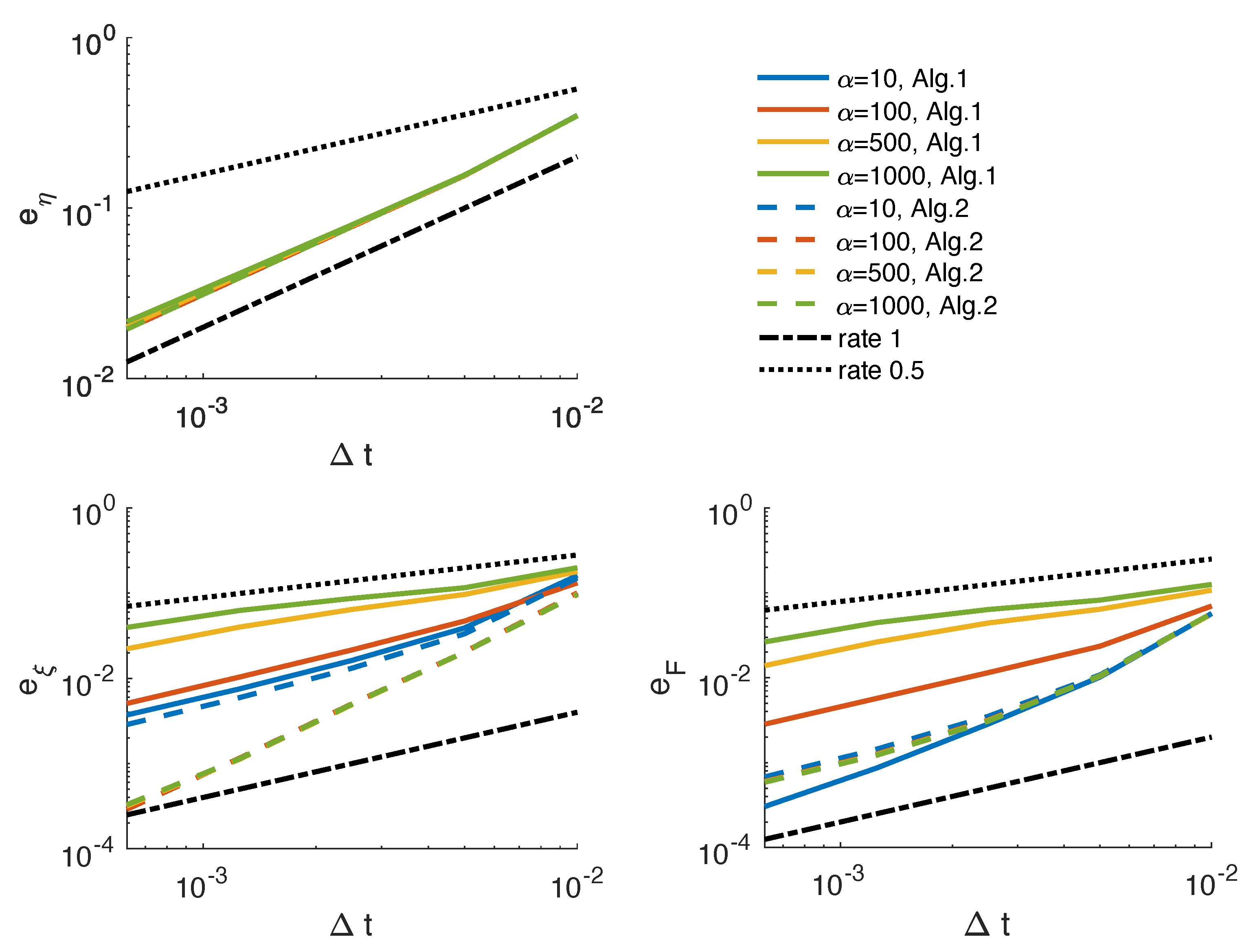
The relative errors obtained using parameters (39) and $\alpha =10,100,500$ and 1000 are shown in Figure 2. The results obtained using Algorithm 2 are shown using dashed lines, while the results obtained using Algorithm 1 are shown using solid lines. Very slight differences in the errors for the structure displacement can be seen for all the considered cases, maintaining a first-order rate of convergence. When Algorithm 1 is used, the relative errors increase as $\alpha$ increases for both structure and fluid velocities. When Algorithm 2 is applied, the relative errors for the structure velocity differ between $\alpha =10$ and the other values of $\alpha$, for which the errors are significantly smaller. In both cases, the errors are smaller than the ones obtained using Algorithm 1. The relative errors for the fluid velocity are similar across different values of $\alpha$, and  just slightly larger than one ones obtained using Algorithm 1 and $\alpha =10$.

The rates of convergence for the solid and fluid velocities, which can be seen in Figure 2, are also given in

Table 1. The rates of convergences obtained using Algorithm 2 and Algorithm 1 with discretization parameters (39).

$\mathit{\alpha }:$	10	100	500	1000	10	100	500	1000
Algorithm 1	$\xi$				$\mathit{u}$
$\Delta t$	-	-	-	-	-	-	-	-
$\Delta t/2$	2.04	1.49	0.89	0.78	2.48	1.57	0.74	0.61
$\Delta t/4$	1.27	1.12	0.58	0.41	1.84	1.03	0.54	0.37
$\Delta t/8$	1.11	1.06	0.69	0.47	1.72	1.01	0.75	0.51
$\Delta t/16$	1.02	1.03	0.85	0.66	1.5	1.01	0.92	0.75
Algorithm 2	$\xi$				$\mathit{u}$
$\Delta t$	-	-	-	-	-	-	-	-
$\Delta t/2$	2.18	2.30	2.26	2.24	2.4	2.43	2.44	2.44
$\Delta t/4$	1.34	2.02	2.05	2.03	1.62	1.72	1.74	1.78
$\Delta t/8$	1.15	2.12	2.13	2.13	1.28	1.33	1.33	1.34
$\Delta t/16$	1.05	1.99	1.81	1.79	1.08	1.07	1.06	1.05

in order to provide a more precise comparison. We observe that for $\alpha =500$ and 1000, the rates become suboptimal when Algorithm 1 is used. However, the rates obtained using Algorithm 2 remain $\mathcal{O}(\Delta t)$ or larger across all values of $\alpha$, and are mostly unaffected when $\alpha$ is changing, with the exception of $\alpha =10$ for the structure velocity.

We also compute the relative errors and rates of convergence using a second set of parameters,

$$\begin{array}{c}(\Delta t,h)\in {\left\{\left(\frac{5·{10}^{-2}}{2^k},\frac{2·{10}^{-1}}{2^k}\right)\right\}}_{k=0}^4,\end{array}$$

(40)

where the time and space discretization parameters are closer in size.

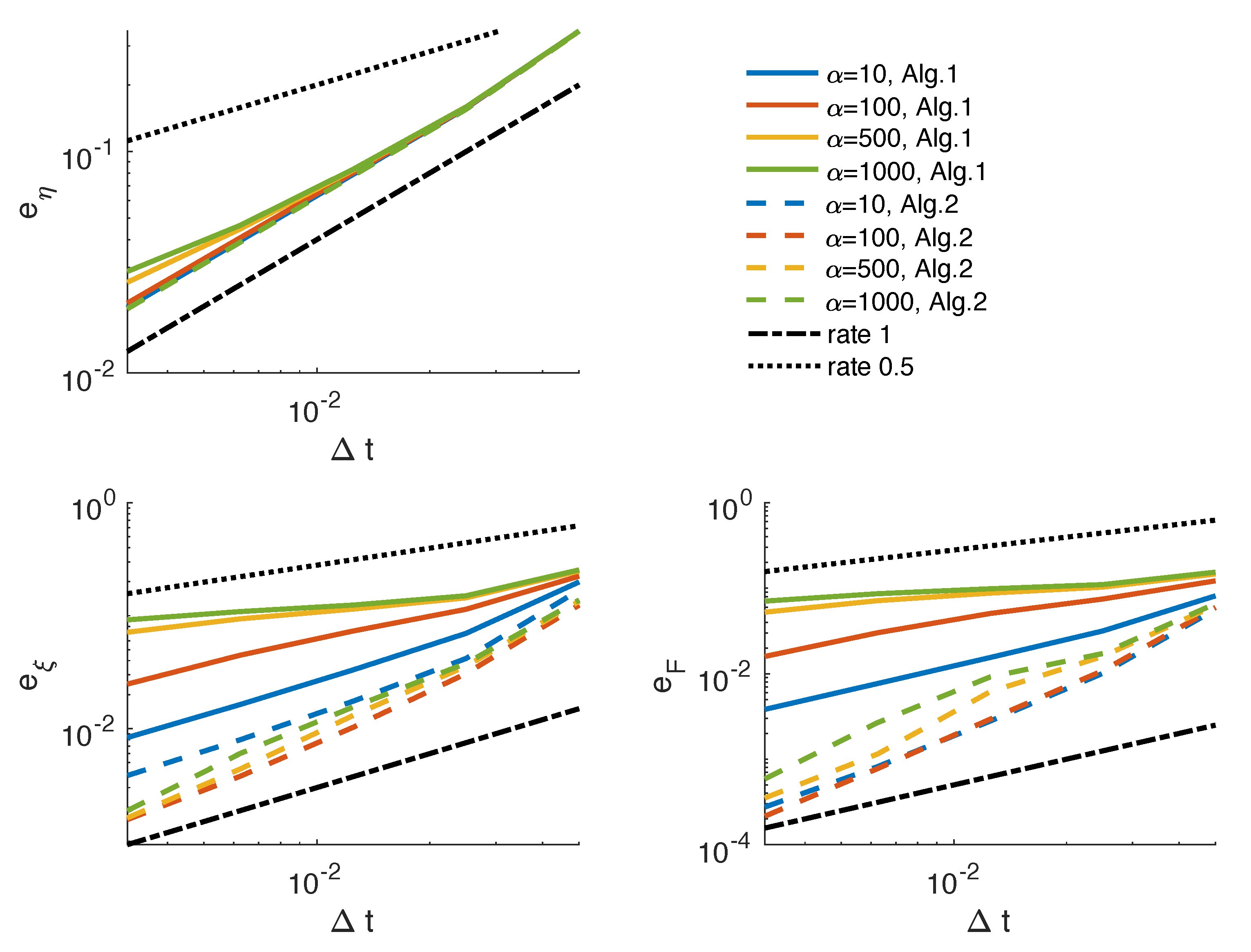
The relative errors obtained using this set of discretization data are shown in Figure 3. The errors for the structure displacement are still close together, but with slight sub-optimalities present in the results obtained using Algorithm 1. Larger differences are observed in the errors for the solid and fluid velocities obtained using Algorithm 2 for different values of $\alpha$ when compared to the ones in Figure 2, with the errors increasing as $\alpha$ increases. However, the errors obtained using Algorithm 2 are smaller in magnitude than the ones obtained using Algorithm 1.

The rates for the solid and fluid velocities obtained using Algorithm 2 and Algorithm 1 with discretization parameters (40) are given in

Table 2. The rates of convergences obtained using Algorithm 2 and Algorithm 1 with discretization parameters (40).

$\mathit{\alpha }:$	10	100	500	1000	10	100	500	1000
Algorithm 1	$\xi$				$\mathit{u}$
$\Delta t$	-	-	-	-	-	-	-	-
$\Delta t/2$	1.51	0.97	0. 79	0.76	1.36	0.71	0.51	0.48
$\Delta t/4$	1.08	0.64	0.33	0.27	1.03	0.56	0.23	0.16
$\Delta t/8$	1.02	0.71	0.29	0.19	1.01	0.75	0.29	0.19
$\Delta t/16$	0.97	0.85	0.39	0.24	1.0	0.92	0.45	0.29
Algorithm 2	$\xi$				$\mathit{u}$
$\Delta t$	-	-	-	-	-	-	-	-
$\Delta t/2$	2.01	2.01	1.91	1.86	2.48	2.45	1.98	1.94
$\Delta t/4$	1.26	1.58	1.45	1.28	1.86	1.89	1.37	0.91
$\Delta t/8$	1.13	1.44	1.58	1.37	1.77	1.92	2.42	1.78
$\Delta t/16$	1.05	1.28	1.44	1.69	1.57	1.85	1.71	2.18

. In this case, Algorithm 1 produces sub-optimal rates even when $\alpha =100,$ with the rates further degrading as $\alpha$ increases. However, the rates obtained using Algorithm 2 remain $\mathcal{O}(\Delta t)$.

4.2. Example 2

In the second example, we use a moving domain model to study the pressure propagation in a two-dimensional channel, commonly used to validate FSI solvers [24]. The reference fluid domain is a rectangle defined by ${\widehat{\Omega }}_F=(0,6)\times (0,0.5)$, interacting with a deformable wall ${\widehat{\Omega }}_S=(0,5)\times (0.5,0.6)$. We consider the FSI problem described in Section 2, where we add a linear “spring” term, $\gamma \mathit{\eta }$, to the elastodynamic Equation (5), yielding

$$\begin{array}{c}\hfill {\rho }_S{\partial }_t\xi +\gamma \mathit{\eta }=\nabla ·{\sigma }_S\left(\mathit{\eta }\right)\mathrm{in}{\widehat{\Omega }}_S\times (0,T).\end{array}$$

The term $\gamma \mathit{\eta }$, obtained from the axially symmetric model, represents a spring keeping the top and bottom boundaries in a two-dimensional model connected [24].

The flow is driven by a time-dependent pressure drop at the inlet and outlet sections, prescribed by

$$\begin{array}{ccc}\hfill & {\sigma }_F{\mathit{n}}_F=-p_{in}\left(t\right){\mathit{n}}_F\hfill & \hfill \mathrm{on}{\Gamma }_F^{in}:=\left\{0\right\}\times (0,0.5),\\ \hfill & {\sigma }_F{\mathit{n}}_F=-p_{out}\left(t\right){\mathit{n}}_F\hfill & \hfill \mathrm{on}{\Gamma }_F^{out}:=\left\{6\right\}\times (0,0.5),\end{array}$$

where

$$\begin{array}{c}\hfill p_{in}\left(t\right)=\left\{\begin{array}{cc}{\displaystyle \frac{p_{max}}{2}\left[1-cos\left({\displaystyle \frac{2\pi t}{t_{max}}}\right)\right],}\hfill & \mathrm{if}t\le t_{max}\hfill \\ 0,\hfill & \mathrm{if}t>t_{max}\hfill \end{array}\right.,p_{out}=0,\end{array}$$

for all $t\in (0,T)$. At the bottom fluid boundary we prescribe symmetry conditions given by

$$u_y=0,\frac{\partial u_x}{\partial y}=0.$$

We assume that the structure is fixed at the edges, with zero normal stress at the external boundary. The pressure pulse is in effect for $t_{max}=0.03$ s with maximum pressure $p_{max}=1.333\times {10}^4$ dyne/${\mathrm{cm}}^2$. The final time is $T=12$ ms, and the time step is $\Delta t=5·{10}^{-5}$. The parameter values used in this example are given in

Table 3. Fluid and structural parameters used in Example 2.

Parameters	Values	Parameters	Values
Fluid density ${\rho }_f$ (g/cm${}^3$)	1	Dyn. viscosity $\mu$ (poise)	$0.035$
Wall density ${\rho }_s$(g/cm${}^3$)	$1.1$	Spring coeff. $\gamma$(dynes/cm${}^4$)	$4\times {10}^6$
Shear mod. ${\mu }_S$ (dyne/cm${}^2$)	$5.575\times {10}^5$	Lamé’s 1st par. ${\lambda }_S$ (dyne/cm${}^2$)	$1.7\times {10}^6$

.

We use ${\mathbb{P}}_2-{\mathbb{P}}_1$ elements for the fluid velocity and pressure, respectively, and  ${\mathbb{P}}_2$ elements for the structure velocity and displacement on a mesh containing 7500 elements in the fluid domain and 1200 elements in the structure domain. As in the previous example, the pressure stabilization is not needed in order to satisfy the inf-sup condition, and hence no pressure stabilization was used.

Choosing the combination parameter $\alpha$ is not trivial. For example, taking $\alpha =0$ in Equation (12) yields the dynamic coupling condition. On the other side, $\alpha =\infty$ recovers the kinematic condition. Hence, we propose to update $\alpha$ dynamically by measuring the errors in the approximations of the kinematic and dynamic coupling conditions so that both conditions are satisfied with comparable accuracy. Therefore, we consider the following two formulas to update $\alpha$ at every time step

$$\begin{array}{cc}\hfill {\alpha }_1^{new}& ={\alpha }_1^{old}{\left(\frac{e_K}{e_D}\right)}^{\frac{1}{2}},\hfill \end{array}$$

(41)

$$\begin{array}{cc}\hfill {\alpha }_2^{new}& ={\alpha }_2^{old}{\left(\frac{e_K}{e_D}\right)}^{\frac{1}{3}},\hfill \end{array}$$

(42)

where

$$\begin{array}{c}\hfill e_K=\frac{{\parallel J(\xi -\mathit{u})\parallel }_{L^2\left(\widehat{\Gamma }\right)}}{{\parallel J\mathit{u}\parallel }_{L^2\left(\widehat{\Gamma }\right)}},e_D=\frac{\parallel J{\sigma }_F{\mathit{F}}^{-T}{\mathit{n}}_F+{\sigma }_S{\mathit{n}}_S{\parallel }_{L^2\left(\widehat{\Gamma }\right)}}{\parallel J{\sigma }_F{\mathit{F}}^{-T}{\mathit{n}}_F{\parallel }_{L^2\left(\widehat{\Gamma }\right)}}.\end{array}$$

We note that in other studies where similar combination parameters are introduced, such as [17], the authors suggest to use

$$\begin{array}{c}\alpha =\frac{{\rho }_S{H}_S}{\Delta t}+\beta H_S\Delta t,\end{array}$$

(43)

where $H_S$ is the height of the solid domain and

$$\beta =\frac{E}{1-{\nu }^2}(4{\rho }_1^2-2(1-\nu ){\rho }_2^2),$$

with E denoting the Young’s modulus, $\nu$ denoting the Poisson’s ratio and ${\rho }_1$ and ${\rho }_2$ denoting the mean and Gaussian curvatures of the fluid–structure interface, respectively. However, this choice of $\alpha$ is proposed to obtain faster convergence of sub-iterative methods for strongly coupled FSI problems. Since we do not require sub-iterations to achieve stability, we do not need similar conditions on $\alpha$. Indeed, it was noted in [9] that using Algorithm 1 with $\alpha$ computed according to (43) yields results that exhibit a larger error that one ones obtained using other values of $\alpha$. Hence, we do not consider Formula (43) in this study.

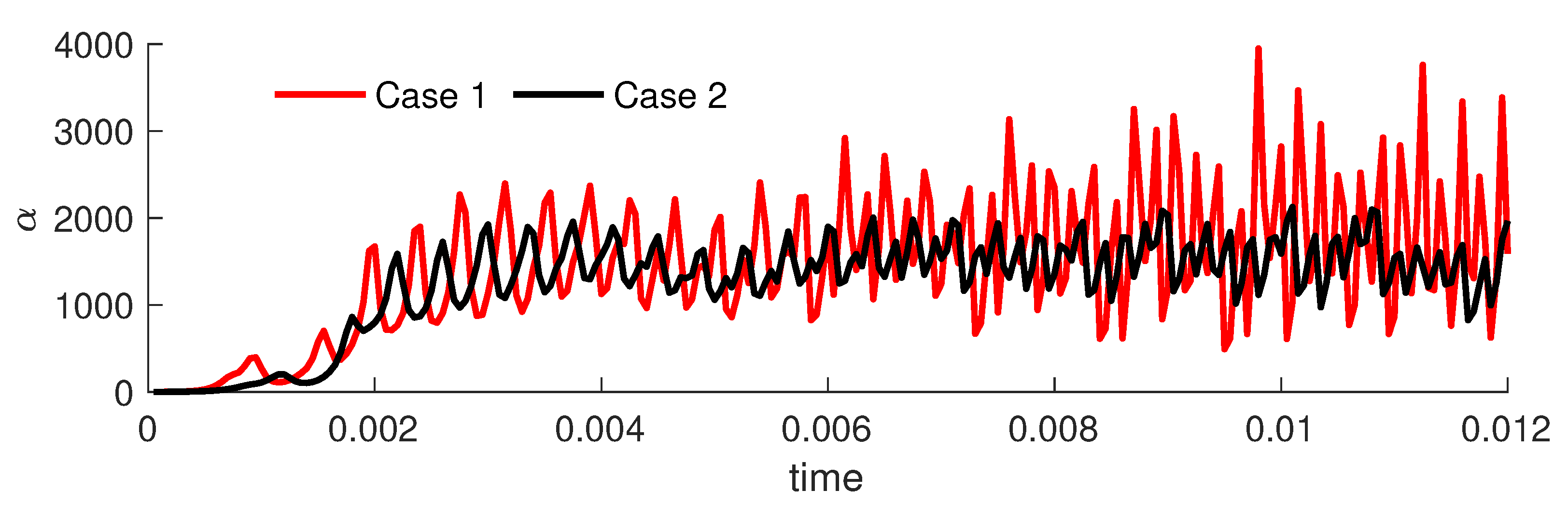
We solve the problem using Algorithm 3 with initial $\alpha =1$, which is then updated according to the given fomulas. The evolution of $\alpha$ obtained by two different cases is shown in Figure 4.

The results indicate that the values of $\alpha$ obtained using (41) (Case 1) exhibit larger oscillations than the ones obtained using (42) (Case 2). For the majority of the simulation, the values of $\alpha$ in Case 1 grow, with the final range between 600 and 4000, and show smaller oscillations in Case 2, with the values between 1000 and 2000.

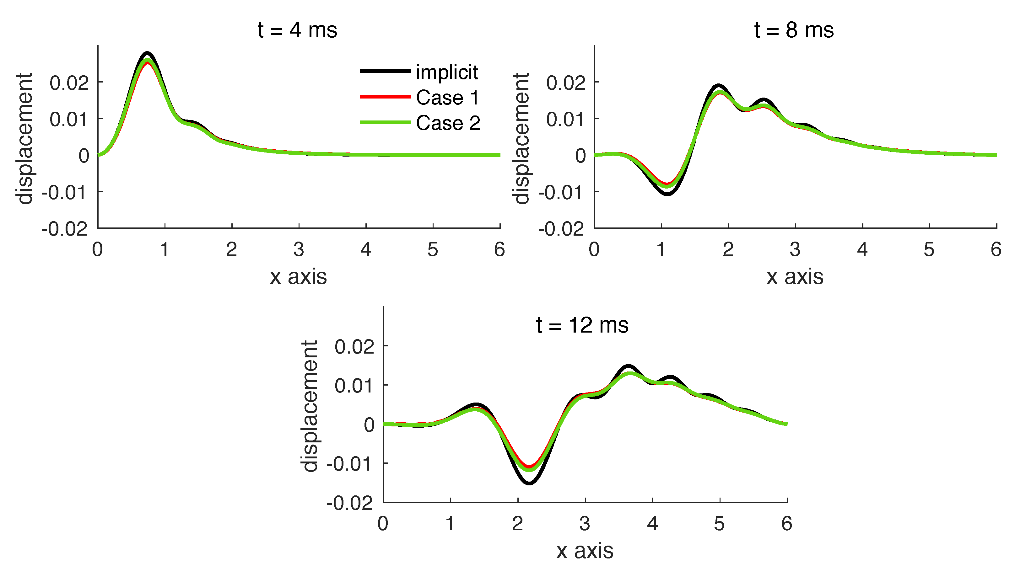
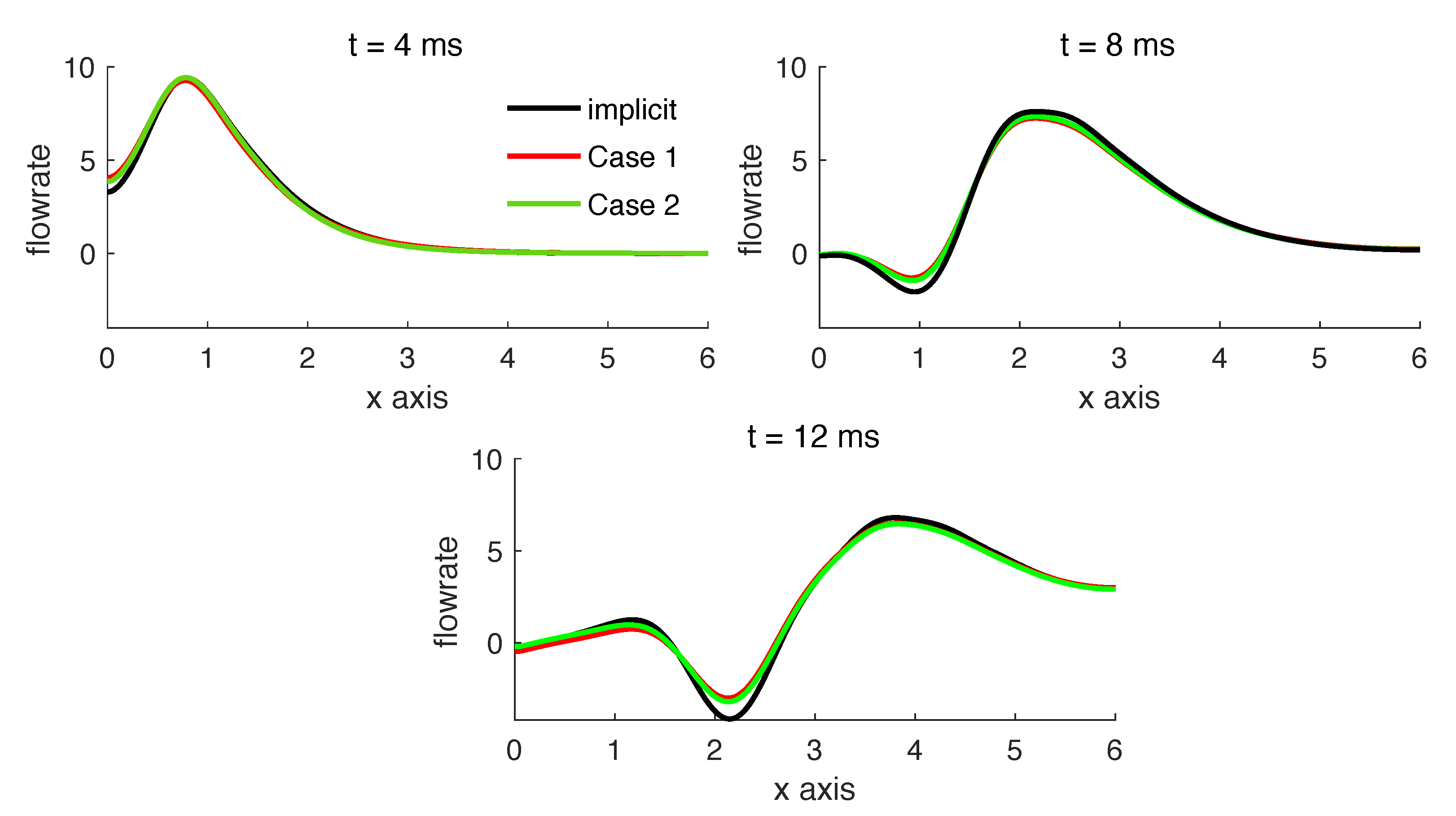
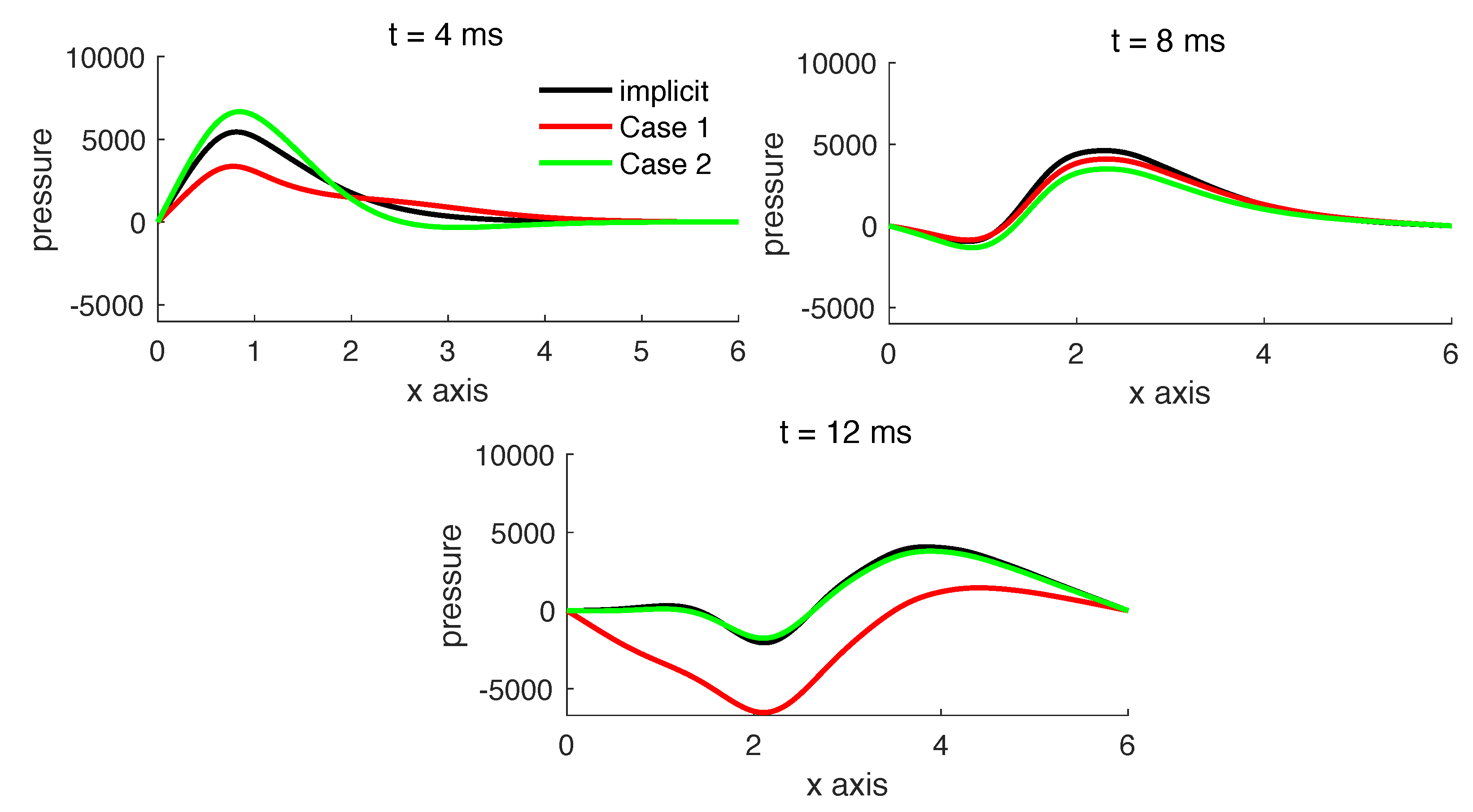
The comparison of the structure displacement, flowrate and pressure along the bottom boundary is shown in Figure 5, Figure 6 and Figure 7, respectively. The results are compared with the ones obtained using an implicit solver, which serve as a reference solution. For the displacement and flowrate, we can observe small improvement in the solution when Case 2 is used instead of Case 1, but both results provide a good comparison with the reference solution. However, there are large variations in the approximations of the fluid pressure. Overall, Case 2 still provides a more accurate solution than Case 1. However, there is still a significant error present when Case 2 is used, especially at time t = 4 ms.

Algorithm 3 Given ${\mathit{u}}^0$ in ${\widehat{\Omega }}_F$, and ${\mathit{\eta }}^0,{\xi }^0$ in ${\widehat{\Omega }}_S$, we first need to compute $p^1,{\mathit{u}}^1$ in ${\Omega }_F\left(t^1\right)$, and ${\mathit{\eta }}^1,{\xi }^1$ in ${\widehat{\Omega }}_S$. A monolithic method could be used. Then, for all $n\ge 2$, compute the following steps:

Structure sub-problem: Find ${\mathit{\eta }}^{n+1}$ and ${\xi }^{n+1}=d_t{\mathit{\eta }}^{n+1}$ such that $$\begin{array}{ccc}\hfill & {\rho }_S{d}_t{\xi }^{n+1}=\nabla ·{\sigma }_S\left({\mathit{\eta }}^{n+1}\right)+{\mathit{f}}_S\left(t^{n+1}\right)\hfill & \hfill \mathrm{in}{\widehat{\Omega }}_S,\\ \hfill & \alpha J^n{\xi }^{n+1}+{\sigma }_S\left({\mathit{\eta }}^{n+1}\right){\mathit{n}}_S=\alpha \delta {\left(J\mathit{u}\right)}^n-2J^n{\sigma }_F({\mathit{u}}^n,p^n){\left({\mathit{F}}^{-T}\right)}^n{\mathit{n}}_F\hfill \\ \hfill & +J^{n-1}{\sigma }_F({\mathit{u}}^{n-1},p^{n-1}){\left({\mathit{F}}^{-T}\right)}^{n-1}{\mathit{n}}_F\hfill & \hfill \mathrm{on}\widehat{\Gamma },\\ \hfill & {\mathit{\eta }}^{n+1}={\mathit{\eta }}_D\left(t^{n+1}\right)\hfill & \hfill \mathrm{on}{\widehat{\Gamma }}_S^D,\\ \hfill & {\sigma }_S\left({\mathit{\eta }}^{n+1}\right){\mathit{n}}_S={\mathit{g}}_S\left(t^{n+1}\right)\hfill & \hfill \mathrm{on}{\widehat{\Gamma }}_S^N.\end{array}$$ Geometry sub-problem: Find ${\mathit{\eta }}_F^{n+1}$ such that $$\begin{array}{ccc}\hfill & -\Delta {\mathit{\eta }}_F^{n+1}=0\hfill & \hfill \mathrm{in}{\widehat{\Omega }}_F,\\ \hfill & {\mathit{\eta }}_F^{n+1}=0\hfill & \hfill \mathrm{on}{\widehat{\Gamma }}_F^D\cup {\widehat{\Gamma }}_F^N,\\ \hfill & {\mathit{\eta }}_F^{n+1}={\mathit{\eta }}^{n+1}\hfill & \hfill \mathrm{on}\widehat{\Gamma },\end{array}$$ and ${\mathit{w}}^{n+1}$ such that $${\mathit{w}}^{n+1}\circ \mathcal{A}\left(t^{n+1}\right)=d_t{\mathit{\eta }}_F^{n+1}\mathrm{in}{\widehat{\Omega }}_F.$$ Compute ${\Omega }_F\left(t^{n+1}\right)$ as ${\Omega }_F\left(t^{n+1}\right)=(I+{\mathit{\eta }}_F^{n+1})\left({\widehat{\Omega }}_F\right)$. Fluid sub-problem: Find ${\mathit{u}}^{n+1}$ and $p^{n+1}$ such that $$\begin{array}{ccc}\hfill & {\rho }_F\left(d_t{\mathit{u}}^{n+1}+({\mathit{u}}^n-{\mathit{w}}^{n+1})·\nabla {\mathit{u}}^{n+1}\right)=\nabla ·{\sigma }_F({\mathit{u}}^{n+1},p^{n+1})+{\mathit{f}}_F\left(t^{n+1}\right)\hfill & \hfill \mathrm{in}{\Omega }_F\left(t^{n+1}\right),\\ \hfill & \nabla ·{\mathit{u}}^{n+1}=0\hfill & \hfill \mathrm{in}{\Omega }_F\left(t^{n+1}\right),\\ \hfill & \alpha J^{n+1}{\mathit{u}}^{n+1}+J^{n+1}{\sigma }_F({\mathit{u}}^{n+1},p^{n+1}){\left({\mathit{F}}^{-T}\right)}^{n+1}{\mathit{n}}_F=\alpha J^{n+1}{\xi }^{n+1}\hfill \\ \hfill & -2J^n{\sigma }_F({\mathit{u}}^n,p^n){\left({\mathit{F}}^{-T}\right)}^n{\mathit{n}}_F+J^{n-1}{\sigma }_F({\mathit{u}}^{n-1},p^{n-1}){\left({\mathit{F}}^{-T}\right)}^{n-1}{\mathit{n}}_F\hfill & \hfill \mathrm{on}\widehat{\Gamma },\\ \hfill & {\mathit{u}}^{n+1}={\mathit{u}}_D\left(t^{n+1}\right)\hfill & \hfill \mathrm{on}{\Gamma }_F^D\left(t^{n+1}\right),\\ \hfill & {\sigma }_F({\mathit{u}}^{n+1},p^{n+1}){\mathit{n}}_F={\mathit{g}}_F\left(t^{n+1}\right)\hfill & \hfill \mathrm{on}{\Gamma }_F^N\left(t^{n+1}\right).\end{array}$$

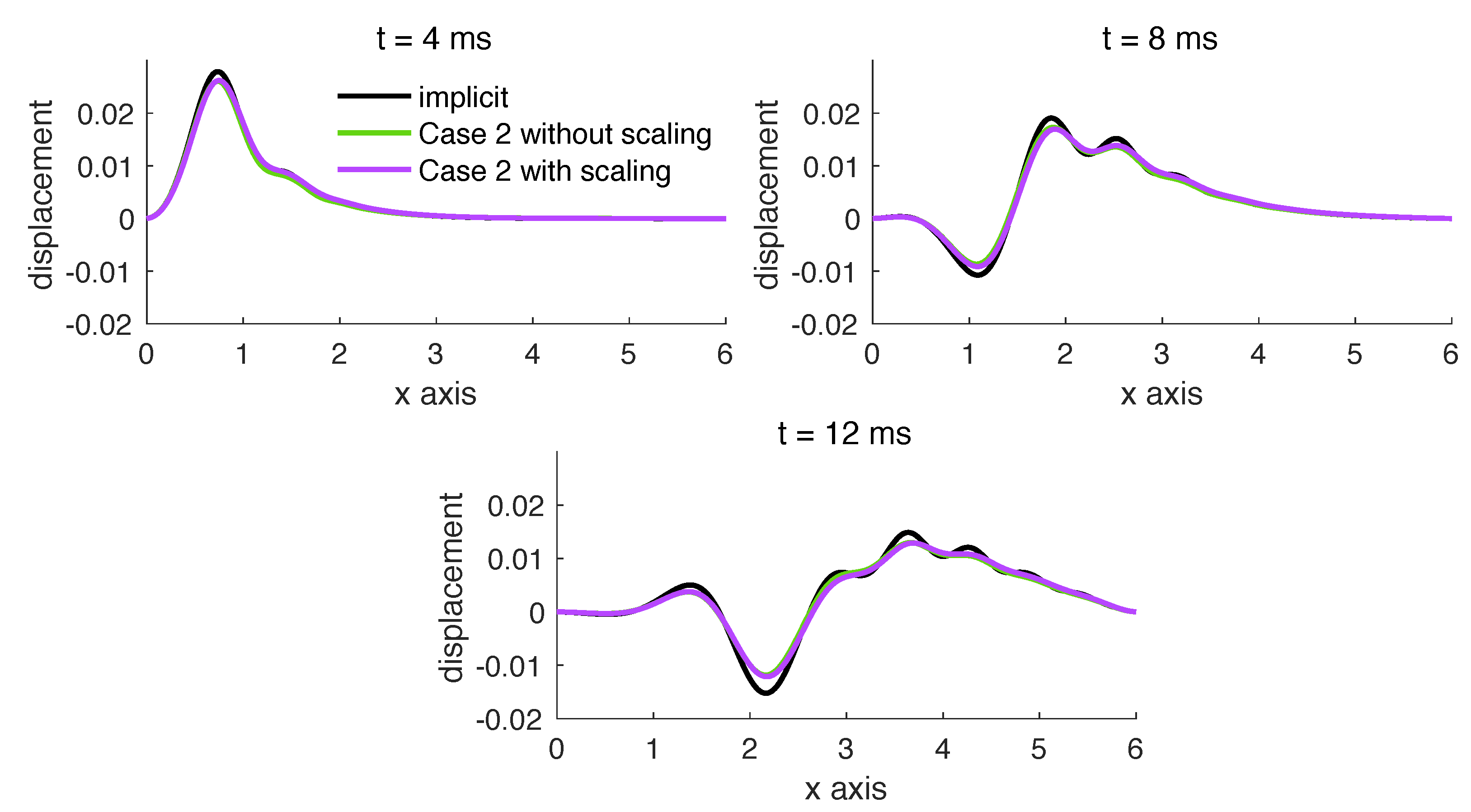
To improve the solution, we revisit the suggested dynamic updates of $\alpha$ and propose to add a scaling factor, which will provide a preference to one of the coupling conditions. In practice, the kinematic coupling condition is often imposed using large penalty parameters (for example, when Nitche’s method is used [6]). Since the results obtained in Case 2 provide a better approximation than the ones in Case 1, we consider only (42), but modify it to include a scaling parameter $\gamma$ as follows

$$\begin{array}{cc}\hfill {\alpha }_3^{new}& ={\alpha }_3^{old}{\left(\frac{\gamma e_K}{e_D}\right)}^{\frac{1}{3}}.\hfill \end{array}$$

(44)

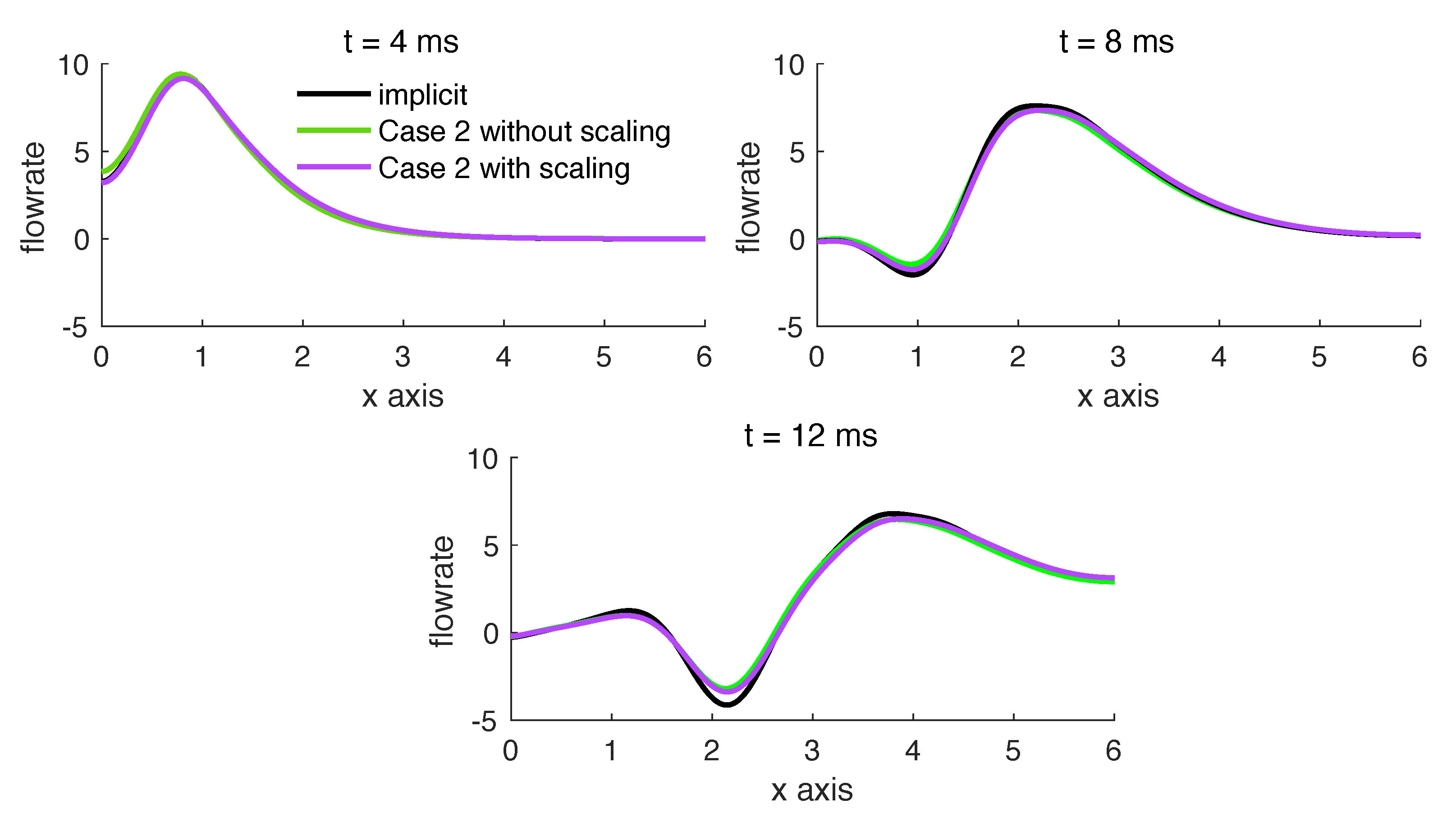
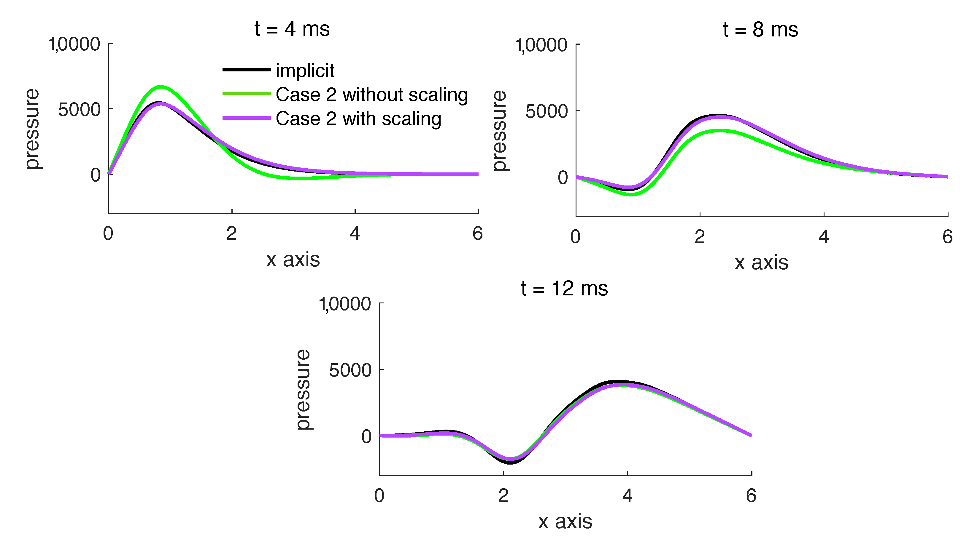
Figure 8, Figure 9 and Figure 10 show the displacement, flowrate and pressure along the bottom boundary, respectively, obtained using an implicit method, Algorithm 3 where $\alpha$ was updated according to (42), and Algorithm 3 where $\alpha$ was updated according to (44) with $\gamma =10$.

We can observe that the displacement does not change significantly when (42) and (44) are used, and the flowrate shows a small improvement when (44) is used instead of (42). However, a major improvement is obtained in the pressure approximation when the scaling is used. All the results provide a good comparison with the implicit solution.

Finally, Figure 11 shows the evolution of $\alpha$ obtained using (42) and (44). We note that the main difference in the results is at the beginning of the simulation, when (44) predicts much larger values of $\alpha$ than (42), which helps to improve the approximation of the pressure at the beginning of the simulation, and subsequently.

5. Conclusions

In this work, we presented an extension of the loosely coupled method for FSI problems presented in [9]. The proposed extension is designed to improve the sub-optimal convergence in time present in the original method. Our stability analysis showed that the proposed method is stable under certain conditions. Even though these conditions are restrictive, our computational results indicate that they are not required to hold in order to obtain numerical stability. Furthermore, our results show that the optimal convergence is restored when the proposed scheme is used, also providing a smaller error in almost all cases considered in this study.

Since the method depends on the combination parameter, $\alpha$, which is problem-dependent and difficult to determine in different applications, we propose a formula for its computation. We computationally investigated several formulas, and showed that the formula based on the scaled ratio of the errors in the approximation of the kinematic and dynamic coupling conditions provides a good agreement between the computed results and the reference solution.

References

- Hou, G.; Wang, J.; Layton, A. Numerical methods for fluid-structure interaction: A review. Commun. Comput. Phys. 2012, 12, 337–377. [Google Scholar] [CrossRef]
- Gee, M.; Küttler, U.; Wall, W. Truly monolithic algebraic multigrid for fluid–structure interaction. Int. J. Numer. Methods Eng. 2011, 85, 987–1016. [Google Scholar] [CrossRef]
- Badia, S.; Quaini, A.; Quarteroni, A. Modular vs. non-modular preconditioners for fluid–structure systems with large added-mass effect. Comput. Methods Appl. Mech. Eng. 2008, 197, 4216–4232. [Google Scholar] [CrossRef] [Green Version]
- Heil, M.; Hazel, A.; Boyle, J. Solvers for large-displacement fluid–structure interaction problems: Segregated versus monolithic approaches. Comput. Mech. 2008, 43, 91–101. [Google Scholar] [CrossRef]
- Burman, E.; Durst, R.; Fernández, M.; Guzmán, J. Fully discrete loosely coupled Robin-Robin scheme for incompressible fluid-structure interaction: Stability and error analysis. arXiv 2020, arXiv:2007.03846. [Google Scholar]
- Burman, E.; Fernández, M. Stabilization of explicit coupling in fluid-structure interaction involving fluid incompressibility. Comput. Methods Appl. Mech. Eng. 2009, 198, 766–784. [Google Scholar] [CrossRef] [Green Version]
- Fernández, M.; Mullaert, J.; Vidrascu, M. Generalized Robin–Neumann explicit coupling schemes for incompressible fluid-structure interaction: Stability analysis and numerics. Int. J. Numer. Methods Eng. 2015, 101, 199–229. [Google Scholar] [CrossRef] [Green Version]
- Bukac, M.; Muha, B. Stability and Convergence Analysis of the Extensions of the Kinematically Coupled Scheme for the Fluid-Structure Interaction. SIAM J. Numer. Anal. 2016, 54, 3032–3061. [Google Scholar] [CrossRef]
- Seboldt, A.; Bukač, M. A non-iterative domain decomposition method for the interaction between a fluid and a thick structure. Numer. Methods Partial. Differ. Equations 2021, 37, 2803–2832. [Google Scholar] [CrossRef]
- Oyekole, O.; Trenchea, C.; Bukac, M. A Second-Order in Time Approximation of Fluid-Structure Interaction Problem. SIAM J. Numer. Anal. 2018, 56, 590–613. [Google Scholar] [CrossRef]
- Fernández, M. Incremental displacement-correction schemes for incompressible fluid-structure interaction: Stability and convergence analysis. Numer. Math. 2012, 123, 210–265. [Google Scholar] [CrossRef] [Green Version]
- Lukáčová-Medvid’ová, M.; Rusnáková, G.; Hundertmark-Zaušková, A. Kinematic splitting algorithm for fluid–structure interaction in hemodynamics. Comput. Methods Appl. Mech. Eng. 2013, 265, 83–106. [Google Scholar] [CrossRef]
- Langer, U.; Yang, H. 5. Recent development of robust monolithic fluid-structure interaction solvers. In Fluid-Structure Interaction; De Gruyter: Berlin, Germany, 2017; pp. 169–192. [Google Scholar]
- Nobile, F.; Vergara, C. An effective fluid-structure interaction formulation for vascular dynamics by generalized Robin conditions. SIAM J. Sci. Comput. 2008, 30, 731–763. [Google Scholar] [CrossRef]
- Badia, S.; Nobile, F.; Vergara, C. Robin-Robin preconditioned Krylov methods for fluid-structure interaction problems. Comput. Methods Appl. Mech. Eng. 2009, 198, 2768–2784. [Google Scholar] [CrossRef] [Green Version]
- Badia, S.; Nobile, F.; Vergara, C. Fluid-structure partitioned procedures based on Robin transmission conditions. J. Comput. Phys. 2008, 227, 7027–7051. [Google Scholar] [CrossRef]
- Gerardo-Giorda, L.; Nobile, F.; Vergara, C. Analysis and Optimization of Robin-Robin Partitioned Procedures in Fluid-Structure Interaction Problems. SIAM J. Numer. Anal. 2010, 48, 2091–2116. [Google Scholar] [CrossRef] [Green Version]
- Degroote, J. On the similarity between Dirichlet–Neumann with interface artificial compressibility and Robin–Neumann schemes for the solution of fluid-structure interaction problems. J. Comput. Phys. 2011, 230, 6399–6403. [Google Scholar] [CrossRef] [Green Version]
- Baek, H.; Karniadakis, G. A convergence study of a new partitioned fluid–structure interaction algorithm based on fictitious mass and damping. J. Comput. Phys. 2012, 231, 629–652. [Google Scholar] [CrossRef]
- Yu, Y.; Baek, H.; Karniadakis, G. Generalized fictitious methods for fluid–structure interactions: Analysis and simulations. J. Comput. Phys. 2013, 245, 317–346. [Google Scholar] [CrossRef]
- Burman, E.; Fernández, M. An unfitted Nitsche method for incompressible fluid-structure interaction using overlapping meshes. Comput. Methods Appl. Mech. Eng. 2014, 279, 497–514. [Google Scholar] [CrossRef]
- Banks, J.; Henshaw, W.; Schwendeman, D. An analysis of a new stable partitioned algorithm for FSI problems. Part I: Incompressible flow and elastic solids. J. Comput. Phys. 2014, 269, 108–137. [Google Scholar] [CrossRef]
- Serino, D.; Banks, J.; Henshaw, W.; Schwendeman, D. A stable added-mass partitioned (AMP) algorithm for elastic solids and incompressible flow: Model problem analysis. SIAM J. Sci. Comput. 2019, 41, A2464–A2484. [Google Scholar] [CrossRef]
- Bukač, M.; Čanić, S.; Glowinski, R.; Muha, B.; Quaini, A. A modular, operator-splitting scheme for fluid–structure interaction problems with thick structures. Int. J. Numer. Methods Fluids 2014, 74, 577–604. [Google Scholar] [CrossRef] [Green Version]
- Burman, E.; Fernández, M.A. Explicit strategies for incompressible fluid-structure interaction problems: Nitsche type mortaring versus Robin–Robin coupling. Int. J. Numer. Methods Eng. 2014, 97, 739–758. [Google Scholar] [CrossRef]
- Burman, E.; Durst, R.; Guzman, J. Stability and error analysis of a splitting method using Robin-Robin coupling applied to a fluid-structure interaction problem. arXiv 2019, arXiv:1911.06760. [Google Scholar]
- Hughes, T.; Liu, W.; Zimmermann, T. Lagrangian-Eulerian finite element formulation for incompressible viscous flows. Comput. Methods Appl. Mech. Eng. 1981, 29, 329–349. [Google Scholar] [CrossRef]
- Donea, J. Arbitrary Lagrangian-Eulerian finite element methods. In Computational Methods for Transient Analysis; North-Holland: Amsterdam, The Netherlands, 1983; pp. 473–516. [Google Scholar]
- Nobile, F. Numerical Approximation of Fluid-Structure Interaction Problems with Application to Haemodynamics. Ph.D. Thesis, EPFL, Lausanne, Switzerland, 2001. [Google Scholar]
- Langer, U.; Yang, H. Numerical simulation of fluid–structure interaction problems with hyperelastic models: A monolithic approach. Math. Comput. Simul. 2018, 145, 186–208. [Google Scholar] [CrossRef] [Green Version]
- Bukač, M.; Čanić, S.; Muha, B. A partitioned scheme for fluid–composite structure interaction problems. J. Comput. Phys. 2015, 281, 493–517. [Google Scholar] [CrossRef] [Green Version]
- Formaggia, L.; Quarteroni, A.; Veneziani, A. Cardiovascular Mathematics: Modeling and Simulation of the Circulatory System; Springer Science & Business Media: Berlin/Heidelberg, Germany, 2010; Volume 1. [Google Scholar]
- Girault, V.; Raviart, P.A. Finite Element Methods for Navier–Stokes Equations: Theory and Algorithms; Springer Science & Business Media: Berlin/Heidelberg, Germany, 2012; Volume 5. [Google Scholar]
Figure 1.
Left: Reference domain . Right: Deformed domain .
Figure 2.
Example 1. Errors for the solid displacement (top-left), solid velocity (bottom-left), and fluid velocity (bottom-right) obtained using parameters (39) at the final time s.
Figure 3.
Example 1. Errors for the solid displacement (top-left), solid velocity (bottom-left), and fluid velocity (bottom-right) obtained using parameters (40) at the final time s.
Figure 5.
Example 2. Displacement vs. x-axis obtained with an implicit scheme and Algorithm 3 where is dynamically updated according to (41) and (42).
Figure 6.
Example 2. Flowrate vs. x-axis obtained with an implicit scheme and Algorithm 3 where is dynamically updated according to (41) and (42).
Figure 7.
Example 2. Pressure vs. x-axis obtained with an implicit scheme and Algorithm 3 where is dynamically updated according to (41) and (42).
Figure 8.
Figure 9.
Figure 10.