Statistical Machine Learning in Model Predictive Control of Nonlinear Processes

Abstract

Recurrent neural networks (RNNs) have been widely used to model nonlinear dynamic systems using time-series data. While the training error of neural networks can be rendered sufficiently small in many cases, there is a lack of a general framework to guide construction and determine the generalization accuracy of RNN models to be used in model predictive control systems. In this work, we employ statistical machine learning theory to develop a methodological framework of generalization error bounds for RNNs. The RNN models are then utilized to predict state evolution in model predictive controllers (MPC), under which closed-loop stability is established in a probabilistic manner. A nonlinear chemical process example is used to investigate the impact of training sample size, RNN depth, width, and input time length on the generalization error, along with the analyses of probabilistic closed-loop stability through the closed-loop simulations under Lyapunov-based MPC.

1. Introduction

Modeling large-scale, complex nonlinear processes has been a long-standing research problem in process systems engineering. The traditional approaches to modeling nonlinear processes include data-driven modeling approach with parameters identified from industrial/simulation data [1,2], and first-principles modeling approach based on a fundamental understanding of the underlying physico-chemical phenomena. While traditional first-principles modeling approach has been used extensively in monitoring, control and optimization of chemical processes, it can be time-demanding and inaccurate to model complex nonlinear processes using first-principle modeling tools. Machine learning methods have been increasingly adopted to model complex nonlinear systems due to their ability to model a rich set of nonlinear functions and handle efficiently with big datasets from processes [3,4,5,6,7,8,9,10]. Among many machine learning modeling techniques, recurrent neural network (RNN) is widely used to model nonlinear dynamic systems using time-series data [11,12,13]. While the history of machine learning methods in chemical process control can be traced back to 1990s [14,15,16,17,18], machine learning has become popular again this decade due to a number of reasons such as cheaper computation (mature and efficient libraries/hardware), availability of large datasets, and advanced learning algorithms. Designing MPC systems that utilize machine learning models with well-characterized accuracy is a new frontier in control systems that will impact the next generation of industrial control systems.

Despite the success of machine learning methods in modeling nonlinear chemical processes in the context of MPC, there remain fundamental challenges that limit the implementation of machine-learning-based MPC to real chemical processes. One important challenge is to characterize the generalization ability on unseen data for machine learning models trained using finite training samples. Furthermore, a theoretical analysis of closed-loop stability for MPC using machine learning models needs to be developed via machine learning and control theory. Typically, theoretical developments on machine-learning-based MPC derived closed-loop stability properties based on the assumption of bounded modeling errors. For example, in [9], a Lyapunov-based MPC scheme using RNN models as the prediction model has been developed with guaranteed closed-loop stability by assuming that the RNN models are able to obtain a sufficiently small and bounded testing error. Similarly, a neural Lyapunov MPC that trains a stabilizing nonlinear MPC based on surrogate model and neural-network-based terminal cost was proposed in [19] with stability properties derived by assuming the boundedness of modeling error. Additionally, in [20], a nonparametric machine learning model is implemented together with MPC in which input-to-state stability is evaluated. In [21], a learning-based MPC targeting deterministic linear models is proposed in which safety, stability, and robustness are proved. However, the fundamental question regarding the generalization accuracy of machine learning models in MPC has not been addressed.

Probably approximately correct (PAC) learning theory is a framework that mathematically analyze the generalization ability of machine learning models [22]. Specifically, in PAC learning, given a set of training data, the learner is supposed to choose the optimal hypothesis (i.e., machine learning model) that yields a low generalization error with high probability from a certain class of hypotheses. Therefore, PAC learning theory provides a useful tool that demonstrates under what conditions a learning algorithm will probably output an approximately correct hypothesis. For example, in [23], PAC learning theory was used to study the learnability of compression learning algorithm for the optimization problem of stochastic MPC using a finite number of realizations of the uncertainty. In [24], PAC learning was used to analyze the generalization performance of a convex piecewise linear classifier that classifies the thermal comfort in a HVAC system. However, to the best of our knowledge, the use of statistical machine learning theory in analyzing stability properties of machine learning models in MPC, and guiding machine learning model structure and training data collection have not been fully explored.

Many recent works have been developed characterizing learnability of neural networks in terms of sample complexity and generalization error [25,26,27,28,29,30,31,32]. Generalization error bound is a common methodology in statistical machine learning for evaluating the predictive performance of machine learning algorithms [33]. This bound depends on a number of factors such as the number of data samples, the number of layers and neurons, bounds of weight matrices, initialization method, among others. For example, in [29], a generalization error bound was developed for a family of RNN models including vanilla RNNs, long short term memory and minimal gated unit. The generalization error bound was established for multiclass classification problems, and was dependent on the total number of network parameters and the spectral norms of the weight matrices. In [27], a sample complexity bound that was fully independent of network depth and width under some assumptions was developed for feedforward neural networks. In [34], an expected risk bound was developed for RNNs that model single-output nonlinear dynamic systems. However, at this stage, generalization error bounds for RNNs that model multiple-input and multiple-output (MIMO) nonlinear dynamic systems using time-series data have not been studied.

Motivated by the above, in this work, we develop the methodological framework of generalization error bounds from machine learning theory for the development and verification of RNN models with specific theoretical accuracy guarantees and integrate these models into model predictive control system design for nonlinear chemical processes. Specifically, in Section 2, the class of nonlinear systems, the formulation of RNNs, along with some general assumptions on system stabilizability and RNN development are presented. In Section 3, preliminaries including some important definitions and lemmas are first presented, followed by the development of a probabilistic generalization error bound for RNN models accounting for the impact of training data size and the number of neurons and layers on accuracy and guiding network structure selection and training. In Section 4, the RNN models are incorporated in the MPC formulation, under which probabilistic closed-loop stability is derived based on the RNN generalization error bound. Finally, in Section 5, a chemical reactor example is used to demonstrate the impact of training sample size, RNN depth and width, input time length on its generalization error. Additionally, closed-loop simulations are carried out to analyze the probabilistic closed-loop stability and performance.

2. Preliminaries

2.1. Notation

The Frobenius norm of A is denoted by ${∥A∥}_F$. The Euclidean norm of a vector is denoted by the operator $\left|·\right|$ and the weighted Euclidean norm of a vector is denoted by the operator ${\left|·\right|}_Q$ where Q is a positive definite matrix. ${\mathbf{R}}_{+}$ denotes nonnegative real numbers. ${\mathbf{x}}^T$ denotes the transpose of $\mathbf{x}$. The notation $L_{f}V\left(\mathbf{x}\right)$ denotes the standard Lie derivative $L_{f}V\left(\mathbf{x}\right):=\frac{\partial V\left(\mathbf{x}\right)}{\partial x}f\left(\mathbf{x}\right)$. Set subtraction is denoted by "∖", i.e., $A\setminus B:=\{x\in {\mathbf{R}}^n|x\in A,x\notin B\}$. A function $f(·)$ is of class ${\mathcal{C}}^1$ if it is continuously differentiable. A continuous function $\alpha :[0,a)\to [0,\infty )$ belongs to class $\mathcal{K}$ if it is strictly increasing and is zero only when evaluated at zero. A function $f:{\mathbf{R}}^n\to {\mathbf{R}}^m$ is said to be L-Lipschitz, $L\ge 0$, if $\left|f\right(a)-f(b\left)\right|\le L|a-b|$ for all $a,b\in {\mathbf{R}}^n$. $\mathbb{P}\left(A\right)$ denotes the probability that event A will occur. $\mathbb{E}\left[X\right]$ denotes the expected value of a random variable X.

2.2. Class of Systems

The class of continuous-time nonlinear systems considered is described by the following state-space form:

$$\dot{x}=F(x,u):=f\left(x\right)+g\left(x\right)u,x\left(t_0\right)=x_0$$

(1)

where $x\in {\mathbf{R}}^n$ and $u\in {\mathbf{R}}^k$ are the sate vector, and the manipulated input vector. The control action is constrained by $u\in U:=\{u_{min}\le u\le u_{max}\}\subset {\mathbf{R}}^k$, where $u_{min}$ and $u_{max}$ represent the minimum and the maximum value vectors of inputs allowed, respectively. $f(·)$ and $g(·)$ are sufficiently smooth vector and matrix functions of dimensions $n\times 1$, and $n\times k$, respectively. Without loss of generality, the initial time $t_0$ is taken to be zero ($t_0=0$), and it is assumed that $f\left(0\right)=0$, and thus, the origin is a steady-state of the system of Equation (1).

We assume the system of Equation (1) is stabilizable in the sense that there exists a stabilizing controller $u=\mathrm{\Phi }\left(x\right)\in U$ that renders the origin exponentially stable. The stabilizability assumption implies that there exists a ${\mathcal{C}}^1$ control Lyapunov function $V\left(x\right)$ such that for all x in an open neighborhood D around the origin, the following inequalities hold:

$$c_1{\left|x\right|}^2\le V\left(x\right)\le c_2{\left|x\right|}^2,$$

(2)

$$\frac{\partial V\left(x\right)}{\partial x}F(x,\mathrm{\Phi }\left(x\right))\le -c_3{\left|x\right|}^2,$$

(3)

$$\left|\frac{\partial V\left(x\right)}{\partial x}\right|\le c_4\left|x\right|$$

(4)

where $c_1$, $c_2$, $c_3$ and $c_4$ are positive constants. Additionally, the Lipschitz property of $F(x,u)$ and the boundedness of u implies there exist positive constants $M_F$, $L_x,L_x^{{}^{\prime }}$ such that the following inequalities hold for all $x,x^{\prime }\in D$ and $u\in U$:

$$\begin{array}{cc}\hfill & \left|F(x,u)\right|\le M_F\hfill \end{array}$$

(5)

$$\begin{array}{cc}\hfill & |F(x,u)-F(x^{\prime },u)|\le L_x|x-x^{\prime }|\hfill \end{array}$$

(6)

$$\begin{array}{cc}\hfill & \left|\frac{\partial V\left(x\right)}{\partial x}F(x,u)-\frac{\partial V\left(x^{\prime }\right)}{\partial x}F(x^{\prime },u)\right|\le L_x^{{}^{\prime }}|x-x^{\prime }|\hfill \end{array}$$

(7)

Following the data generation method in [9], open-loop simulations of the nonlinear system of Equation (1) are first conducted to generate a large dataset that captures the system dynamics for $x\in {\mathrm{\Omega }}_{\rho }$ and $u\in U$, where ${\mathrm{\Omega }}_{\rho }:=\{x\in {\mathbf{R}}^n|V\left(x\right)\le \rho \}$, $\rho >0$, is a compact set within which the system stability is guaranteed using the controller $u=\mathrm{\Phi }\left(x\right)\in U$. Specifically, we sweep over all the values that $(x,u)$ can take by running extensive open-loop simulations of the system of Equation (1) under various $x_0\in {\mathrm{\Omega }}_{\rho }$ and inputs u to generate a large number of dynamic trajectories. The open-loop simulation of the continuous system of Equation (1) under a sequence of inputs $u\in U$ is carried out in a sample-and-hold fashion (i.e., the inputs are fed into the system of Equation (1) as a piecewise constant function, $u\left(t\right)=u\left(t_k\right)$, $\forall t\in [t_k,t_{k+1})$, where $t_{k+1}:=t_k+\Delta$, and $\Delta$ is the sampling period). The nonlinear system of Equation (1) is integrated via explicit Euler method with a sufficiently small integration time step $h_c<\Delta$. Using the open-loop simulation data, recurrent neural network (RNN) models are developed to predict future states for (at least) one sampling period based on the current state measurements, and the manipulated inputs that will be applied for the next sampling period. In other words, the RNN model is developed to predict $x\left(t\right)$, $\forall t\in [t_k,t_{k+1})$ based on the measurements $x\left(t_k\right)$ and the inputs $u\in [t_k,t_{k+1})$. Finally, the time-series dataset is partitioned into three subsets for the purposes of training, validation and testing.

2.3. Recurrent Neural Network Model

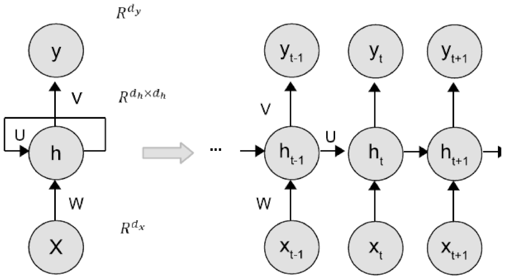
Consider an RNN model that approximates the nonlinear dynamics of the system of Equation (1) with m sequences of T-time-length data points $({\mathbf{x}}_{i,t},{\mathbf{y}}_{i,t})$ where ${\mathbf{x}}_{i,t}\in {\mathbf{R}}^{d_x}$ is the RNN input, and ${\mathbf{y}}_{i,t}\in {\mathbf{R}}^{d_y}$ is the RNN output, $i=1,...,m$ and $t=1,...,T$ (Figure 1). It should be noted that the RNN inputs and outputs do not necessarily represent the nonlinear system inputs and states/outputs in Equation (1). Therefore, to differentiate the notations for RNN inputs/outputs from those for the nonlinear system of Equation (1), all the vectors for RNN models are written in boldface. Additionally, to simplify the discussion, the RNN model of Equations (8) and (9) is developed to predict states over one sampling period with total time steps $T=\frac{\Delta }{h_c}$ (i.e., the RNN model is to predict future states for all the integration time step $h_c$ within one sampling period $\Delta$). As a result, the RNN input ${\mathbf{x}}_{i,t}$ consists of the current state measurements and manipulated inputs that will be applied over $t=1,...,T$, and the RNN output ${\mathbf{y}}_{i,t}$ consists of the predicted states over $t=1,...,T$. Note that ${\mathbf{x}}_{i,t}$ remains unchanged over $t=1,...,T$ due to the sample-and-hold implementation of manipulated inputs.

The dataset is developed consisting of m data sequences drawn independently from some underlying distribution over ${\mathbf{R}}^{d_x\times T}\times {\mathbf{R}}^{d_y\times T}$. In this work, we consider a one-hidden-layer RNN with hidden states ${\mathbf{h}}_i\in {\mathbf{R}}^{d_h}$ computed as follows:

$${\mathbf{h}}_{i,t}={\sigma }_h(U{\mathbf{h}}_{i,t-1}+W{\mathbf{x}}_{i,t})$$

(8)

where ${\sigma }_h$ is the element-wise nonlinear activation function (e.g., ReLU). $U\in {\mathbf{R}}^{d_h\times d_h}$ and $W\in {\mathbf{R}}^{d_h\times d_x}$ are weight matrices connected to the hidden states and input vector, respectively. The output layer ${\mathbf{y}}_{i,t}$ is computed as follows:

$${\mathbf{y}}_{i,t}={\sigma }_y\left(V{\mathbf{h}}_{i,t}\right)$$

(9)

where $V\in {\mathbf{R}}^{d_y\times d_h}$ is the weight matrix, and ${\sigma }_y$ is the element-wise activation function in the output layer (typically linear unit for regression problems).

We consider the loss function $L(\mathbf{y},\overline{\mathbf{y}})$ which calculates the squared difference between the true value $\overline{\mathbf{y}}$ and the predicted value $\mathbf{y}$ (i.e., $L_2$ loss). Without loss of generality, we have the following assumptions on the RNN model and dataset.

Assumption 1.

The RNN inputs are bounded, i.e., $\left|{\mathbf{x}}_{i,t}\right|\le B_X$, for all $i=1,...,m$ and $t=1,...,T$.

Assumption 2.

The Frobenius norms of all the weight matrices are bounded as follows:

$${∥U∥}_F\le B_{U,F},{∥V∥}_F\le B_{V,F},{∥W∥}_F\le B_{W,F}$$

(10)

Assumption 3.

Training, validation, and testing datasets are drawn from the same distribution.

Assumption 4.

The nonlinear activation function ${\sigma }_h$ is 1-Lipschitz continuous, and is positive-homogeneous, i.e., ${\sigma }_h\left(\alpha z\right)=\alpha {\sigma }_h\left(z\right)$ for all $\alpha \ge 0$ and $z\in \mathbf{R}$.

Remark 1.

All the assumptions made are standard in machine learning theory, and can be presented in system-theoretic language as follows. Assumption 1 assumes that the RNN inputs are bounded, which is consistent with the fact that the process states x and inputs u are bounded by $x\in {\mathrm{\Omega }}_{\rho }$ and $u\in U$. Assumption 2 requires the RNN weight matrices to be bounded, which implies that only a finite class of neural network hypotheses are considered for modeling the nonlinear system of Equation (1). Assumption 3 is a natural and necessary assumption for generalization performance analysis. It implies that the machine learning models built from industrial operation data will be applied to the same process with the same data distribution. An example of activation function that satisfies Assumption 4 is Rectified Linear Unit (ReLu), which is a nonlinear activation function that has gained popularity in the machine learning domain.

3. RNN Generalization Error

Since any learning algorithms are evaluated on finite training samples only, and do not provide any information on their predictive performance for unseen data, generalization error provides an important measure of how accurately a neural network model is able to predict output values for input data that has not been used in training. To implement machine learning models into real chemical processes, it is necessary to demonstrate that models are developed with a desired generalization error such that they can be applied for any reasonable operating conditions beyond those in the training dataset while maintaining a sufficiently small modeling error. In this section, we develop an upper bound for the generalization error of RNN models, and demonstrate that this error can be bounded with high probability provided that the training data samples and neural network structure meet a few requirements.

3.1. Preliminaries

We first present some important definitions and lemmas that will be used in the derivation of RNN generalization error. The random variables satisfying sub-Gaussian distribution, which is a probability distribution with strong tail decay, are defined as follows:

Definition 1.

A centered random variable $x\in \mathbf{R}$ is said to be sub-Gaussian with variance proxy ${\sigma }^2$, if $\mathbb{E}\left[x\right]=0$, and the moment generating function satisfies

$$\mathbb{E}[exp\left(aX\right)]\le exp\left(\frac{a^2{\sigma }^2}{2}\right),\forall a\in \mathbf{R}$$

(11)

Lemma 1

(McDiarmid’s inequality [35]). Consider independent random variables $X_1,...,X_n\in X$ and a function $f:X^n\to \mathbf{R}$ with bounded difference property, i.e., there exist positive numbers $c_i$ such that the following inequality holds for all $x_1,...,x_n,x_i^{\prime }\in X$, $x_i\ne x_i^{\prime }$ and $i\in \{1,...,n\}$:

$$|f(x_1,...,x_i,...,x_n)-f(x_1,...,x_i^{\prime },...,x_n)|\le c_i$$

(12)

then the following probability holds for any $a>0$:

$$\mathbb{P}(f(X_1,...,X_n)-\mathbb{E}\left[f(X_1,...,X_n)\right]\ge a)\le exp\left(-\frac{2a^2}{{\sum }_{i=1}^n{c}_i^2}\right)$$

(13)

Let $L({\mathbf{y}}_t,{\overline{\mathbf{y}}}_t)$ be the loss function, where ${\mathbf{y}}_t=h\left({\mathbf{x}}_t\right)$ is the predicted RNN output, and $h(·)$ represents the RNN functions in the hypothesis class $\mathcal{H}$ mapping input $\mathbf{x}\in {\mathbf{R}}^{d_x}$ to output $\mathbf{y}\in {\mathbf{R}}^{d_y}$. The following error definitions are commonly used in machine learning theory.

Definition 2.

Given a function h that predicts output values y for each input x, and an underlying distribution D, theexpected loss/errororgeneralization erroris

$$L_D\left(h\right)\triangleq \mathbb{E}\left[L(h\left(x\right),y)\right]={\int }_{X\times Y}L(h\left(x\right),y)\rho (x,y)dxdy$$

(14)

where $\rho (x,y)$ is joint probability distribution for x and y, and X, Y are the vector space of all possible inputs, and outputs, respectively.

Since in general the joint probability distribution $\rho$ is unknown, we use the data samples drawn from this unknown probability distribution to compute empirical error, which is a proxy measure for the expected loss.

Definition 3.

Given a dataset with m data samples $S=(s_1,...,s_m)$, where $s_i=(x_i,y_i)$, theempirical errororriskis

$${\widehat{\mathbb{E}}}_S\left[L(h\left(x\right),y)\right]=\frac{1}{m}\sum _{i=1}^{m}L(h\left(x_i\right),y_i)$$

(15)

The RNN model is developed by minimizing the empirical risk of Equation (15) using a set of m data sequences. To ensure that the RNN model achieves a desired generalization performance in the sense that it well captures the nonlinear dynamics of the system of Equation (1) for various operation conditions, the objective of this work is to show that the generalization error $\mathbb{E}\left[L\right(h\left(\mathbf{x}\right),\mathbf{y}\left)\right]$ can be bounded provided that the empirical risk is sufficiently small and bounded.

We consider the mean squared error (MSE) as loss function in this work. It is readily shown that the MSE loss function $L(\mathbf{y},\overline{\mathbf{y}})$ is not Lipschitz continuous for all $\mathbf{y},\overline{\mathbf{y}}\in {\mathbf{R}}^{d_y}$. However, since we consider a finite hypothesis class that satisfies Assumptions 1–4, we can show that the RNN output is bounded. This is consistent with the fact that the nonlinear system of Equation (1) is operated in the stability region ${\mathrm{\Omega }}_{\rho }$, and therefore, the RNN outputs are bounded within a compact set.

Let $r_t>0$ denote the upper bound of ${\mathbf{y}}_t$, i.e., $|{\mathbf{y}}_t|\le r_t$, $t=1,...,T$. Without loss of generality, we assume that the true outputs are also bounded by $r_t$. Therefore, the MSE loss function is a locally Lipschitz continuous function satisfying the following inequality for all $|{\mathbf{y}}_t|,|{\overline{\mathbf{y}}}_t|\le r_t$.

$$|L({\mathbf{y}}_1,\overline{\mathbf{y}})-L({\mathbf{y}}_2,\overline{\mathbf{y}})|\le L_r\left|{\mathbf{y}}_1-{\mathbf{y}}_2\right|$$

(16)

where $L_r$ is the local Lipschitz constant.

The generalization error of a neural network function $h_S$ chosen from a hypothesis class $\mathcal{H}$ based on a certain learning algorithm and a training dataset S drawn from distribution D can be decomposed into the approximation error and the estimation error as follows:

$$L_D\left(h_S\right)-L_D\left(h^{\ast }\right)=(\underset{h\in \mathcal{H}}{min}{L}_D\left(h\right)-L_D\left(h^{\ast }\right))+(L_D\left(h_S\right)-\underset{h\in \mathcal{H}}{min}{L}_D\left(h\right))$$

(17)

where the first and second terms in parentheses represent approximation error and estimation error, respectively. Specifically, $L_D\left(h_S\right)$ represents the error evaluated using the hypothesis $h_S$ over the underlying data distribution D. $h^{\ast }$ represents the optimal hypothesis (maybe outside of the finite hypothesis class $\mathcal{H}$) for the data distribution D. ${min}_{h\in \mathcal{H}}{L}_D\left(h\right)$ is the optimal hypothesis within $\mathcal{H}$ that minimizes the loss functions over the distribution D. It can be seen that the approximation error depends on how close the hypothesis class $\mathcal{H}$ is to the optimal hypothesis $h^{\ast }$. In other words, a larger hypothesis class $\mathcal{H}$ generally leads to a lower approximation error since it is more likely that the optimal hypothesis $h^{\ast }$ is included in $\mathcal{H}$. The estimation error depends on both the hypothesis class size and training data, and characterizes how good the selected hypothesis $h_S$ associated with the training dataset S is with respect to the best hypothesis ${min}_{h\in \mathcal{H}}{L}_D\left(h\right)$ within hypothesis class $\mathcal{H}$. As a result, a larger hypothesis class $\mathcal{H}$ may in turn lead to a higher estimation error since it is more difficult to find the optimal hypothesis within $\mathcal{H}$ over the distribution D. From the error decomposition of Equation (17), we demonstrate the dependencies of generalization error on the training dataset size and the complexity of hypothesis class. In the next section, we will take advantage of Rademacher complexity technique to derive a generalization error bound accounting for its dependencies on the above factors in a quantitative aspect. The results will also provide a guide for the design of neural network structures and the collection of training data in order to achieve a desired generalization performance for a specific modeling task.

3.2. Rademacher Complexity Bound

Rademacher complexity quantifies the richness of a class of functions, and is often used in machine learning theory to bound the generalization error. The definition of empirical Rademacher complexity is given below.

Definition 4

(Empirical Rademacher Complexity). Given a hypothesis class $\mathcal{F}$ of real-valued functions, and a set of data samples $S=\{s_1,...,s_m\}$, the empirical Rademacher complexity of $\mathcal{F}$ is defined as

$${\mathcal{R}}_S\left(\mathcal{F}\right)={\mathbb{E}}_{ϵ}\left[\underset{f\in \mathcal{F}}{sup}\frac{1}{m}\sum _{i=1}^m{ϵ}_{i}f\left(s_i\right)\right]$$

(18)

where $ϵ={({ϵ}_1,...,{ϵ}_m)}^T$ with ${ϵ}_i$ being independent and identically distributed (i.i.d.) Rademacher random variables satisfying $\mathbb{P}({ϵ}_i=1)=\mathbb{P}({ϵ}_i=-1)=0.5$.

We also have the following contraction inequality for the hypothesis class $\mathcal{H}$ of vector-valued functions $h\in {\mathbf{R}}^{d_y}$.

Lemma 2

(c.f. Corollary 4 in [36]). Consider a hypothesis class $\mathcal{H}$ of vector-valued functions $h\in {\mathbf{R}}^{d_y}$, and a set of data samples $S=\{s_1,...,s_m\}$. Let $L(·)$ be a $L_r$-Lipschitz function mapping $h\in {\mathbf{R}}^{d_y}$ to $\mathbf{R}$, then we have

$${\mathbb{E}}_{ϵ}\left[\underset{h\in \mathcal{H}}{sup}\sum _{i=1}^m{ϵ}_{i}L(h\left({\mathbf{x}}_i\right),{\mathbf{y}}_i)\right]\le \sqrt{2}{L}_r{\mathbb{E}}_{ϵ}\left[\underset{h\in \mathcal{H}}{sup}\sum _{i=1}^m\sum _{k=1}^{d_y}{ϵ}_{ik}{h}_k\left({\mathbf{x}}_i\right)\right]$$

(19)

where $h_k(·)$ is the k-th component in the vector-valued function $h(·)$, and ${ϵ}_{ik}$ is an $m\times d_y$ matrix of independent Rademacher variables. In the following text, we will omit the subscript ϵ of expectation for simplicity.

Since the RHS of Equation (19) is generally difficult to compute, we can reduce it to scalar classes, and derive the following bound [36]:

$$\mathbb{E}\left[\underset{h\in \mathcal{H}}{sup}\sum _{i=1}^m\sum _{k=1}^{d_y}{ϵ}_{ik}{h}_k\left({\mathbf{x}}_i\right)\right]\le \sum _{k=1}^{d_y}\mathbb{E}\left[\underset{h\in {\mathcal{H}}_k}{sup}\sum _{i=1}^m{ϵ}_{i}h\left({\mathbf{x}}_i\right)\right]$$

(20)

where ${\mathcal{H}}_k$, $k=1,...,d_y$, are classes of scalar-valued functions that correspond to the components of vector-valued functions in $\mathcal{H}$. Equation (20) will later be used in the derivation of the generalization error bound for RNN models approximating the nonlinear system of Equation (1).

Let ${\mathcal{G}}_t$ be the family of loss functions associated to $\mathcal{H}$ mapping the first t-time-step inputs $\{{\mathbf{x}}_1,{\mathbf{x}}_2,...,{\mathbf{x}}_t\}\in {\mathbf{R}}^{d_x\times t}$ to the t-th output ${\mathbf{y}}_t\in {\mathbf{R}}^{d_y}$.

$${\mathcal{G}}_t=\{g_t:(\mathbf{x},\overline{\mathbf{y}})\to L(h\left(\mathbf{x}\right),\overline{\mathbf{y}}),h\in \mathcal{H}\}$$

(21)

where $\mathbf{x}$ is the RNN input vector, and $\overline{\mathbf{y}}$ is the true output vector. The following lemma characterizes the upper bound for the generalization error using Rademacher complexity ${\mathcal{R}}_S\left({\mathcal{G}}_t\right)$.

Lemma 3

(c.f. Theorem 3.3 in [37]). Given a set of m i.i.d. data samples, with probability at least $1-\delta$ over samples $S={({\mathbf{x}}_{i,t},{\mathbf{y}}_{i,t})}_{t=1}^T$, $i=1,...,m$, the following inequality holds for all $g_t\in {\mathcal{G}}_t$:

$$\mathbb{E}\left[g_t(\mathbf{x},\mathbf{y})\right]\le \frac{1}{m}\sum _{i=1}^m{g}_t({\mathbf{x}}_i,{\mathbf{y}}_i)+2{\mathcal{R}}_S\left({\mathcal{G}}_t\right)+3\sqrt{\frac{log\left(\frac{2}{\delta }\right)}{2m}}$$

(22)

Proof. 

While the full proof can be found in many machine learning books, e.g., [37], a proof sketch is presented below to help readers understand the derivation of Equation (22). To simplify the notations, let $\mathbb{E}\left[g_t\right]$ and ${\widehat{\mathbb{E}}}_S\left[g_t\right]$ denote the expected loss $\mathbb{E}\left[g_t(\mathbf{x},\mathbf{y})\right]$ and the empirical loss $\frac{1}{m}{\sum }_{i=1}^m{g}_t({\mathbf{x}}_i,{\mathbf{y}}_i)$ based on a dataset S with m data samples, respectively. Additionally, we assume that $g_t(\mathbf{x},\mathbf{y})$ is bounded in $[0,1]$ (if not, we can scale the RNN output layer or loss function) without loss of generality. We define $\beta \left(S\right)$ to be a function of data samples $S=(s_1,s_2,...,s_m)$ as follows, where $s_i$ represents each data sample $({\mathbf{x}}_{i,t},{\mathbf{y}}_{i,t})$, $i=1,...,m$.

$$\beta \left(S\right)=\underset{g_t\in {\mathcal{G}}_t}{sup}(\mathbb{E}\left[g_t\right]-{\widehat{\mathbb{E}}}_S\left[g_t\right])$$

(23)

Given two datasets $S=(s_1,...,s_i,...,s_m)$ and $S^{\prime }=(s_1,...,s_i^{\prime },...,s_m)$ with only one different data point, i.e., $s_i\ne s_i^{\prime }$, the following inequality holds for any $g_t({\mathbf{x}}_i,{\mathbf{y}}_i)\in [0,1]$:

$$\begin{array}{cc}\hfill \left|\beta \left(S\right)-\beta \left(S^{\prime }\right)\right|& =\left|\underset{g_t\in {\mathcal{G}}_t}{sup}(\mathbb{E}\left[g_t\right]-{\widehat{\mathbb{E}}}_S\left[g_t\right])-\underset{g_t\in {\mathcal{G}}_t}{sup}(\mathbb{E}\left[g_t\right]-{\widehat{\mathbb{E}}}_{S^{\prime }}\left[g_t\right])\right|\hfill \\ \hfill & \le \left|\underset{g_t\in {\mathcal{G}}_t}{sup}({\widehat{\mathbb{E}}}_{S^{\prime }}\left[g_t\right]-{\widehat{\mathbb{E}}}_S\left[g_t\right])\right|\hfill \\ \hfill & =\left|\underset{g_t\in {\mathcal{G}}_t}{sup}\frac{g_t\left(s_i^{\prime }\right)-g_t\left(s_i\right)}{m}\right|\hfill \\ \hfill & \le \frac{1}{m}\hfill \end{array}$$

(24)

Then, using the McDiarmid’s inequality in Lemma 1 and letting $a\ge \sqrt{\frac{log\left(\frac{2}{\delta }\right)}{2m}}$, we have

$$\mathbb{P}[\beta \left(S\right)-{\mathbb{E}}_S\left[\beta \left(S\right)\right]\ge a]\le exp\left(\frac{-2a^2}{{\sum }_{i=1}^m\frac{1}{m^2}}\right)=exp(-2a^{2}m)\le \frac{\delta }{2}$$

(25)

where ${\mathbb{E}}_S\left[\beta \left(S\right)\right]$ denotes the expectation of $\beta \left(S\right)$ with respect to the dataset S of m data samples. Equivalently, the following inequality holds with probability at least $1-\frac{\delta }{2}$, for any $\delta >0$:

$$\beta \left(S\right)\le {\mathbb{E}}_S\left[\beta \left(S\right)\right]+\sqrt{\frac{log\left(\frac{2}{\delta }\right)}{2m}}$$

(26)

Next, we derive the upper bound for ${\mathbb{E}}_S\left[\beta \left(S\right)\right]$ as follows:

$$\begin{array}{cc}\hfill {\mathbb{E}}_S\left[\beta \left(S\right)\right]& ={\mathbb{E}}_S\left[\underset{g_t\in {\mathcal{G}}_t}{sup}(\mathbb{E}\left[g_t\right]-{\widehat{\mathbb{E}}}_S\left[g_t\right])\right]\hfill \\ \hfill & \le {\mathbb{E}}_{S,S^{\prime }}\left[\underset{g_t\in {\mathcal{G}}_t}{sup}({\widehat{\mathbb{E}}}_{S^{\prime }}\left[g_t\right]-{\widehat{\mathbb{E}}}_S\left[g_t\right])\right]\hfill \\ \hfill & ={\mathbb{E}}_{ϵ,S,S^{\prime }}\left[\underset{g_t\in {\mathcal{G}}_t}{sup}\left(\frac{1}{m}\sum _{i=1}^m{ϵ}_i(g_t\left(s_i^{\prime }\right)-g_t\left(s_i\right))\right)\right]\hfill \\ \hfill & \le {\mathbb{E}}_{ϵ,S^{\prime }}\left[\underset{g_t\in {\mathcal{G}}_t}{sup}\left(\frac{1}{m}\sum _{i=1}^m{ϵ}_i{g}_t\left(s_i^{\prime }\right)\right)\right]+{\mathbb{E}}_{ϵ,S}\left[\underset{g_t\in {\mathcal{G}}_t}{sup}\left(\frac{1}{m}\sum _{i=1}^m-{ϵ}_i{g}_t\left(s_i\right)\right)\right]\hfill \\ \hfill & =2{\mathbb{E}}_{ϵ,S}\left[\underset{g_t\in {\mathcal{G}}_t}{sup}\frac{1}{m}\sum _{i=1}^m{ϵ}_i{g}_t\left(s_i\right)\right]=2{\mathbb{E}}_{ϵ,S}\left[{\mathcal{R}}_S\left({\mathcal{G}}_t\right)\right]\hfill \end{array}$$

(27)

where the first line is by substituting the definition of Equation (23) into ${\mathbb{E}}_S\left[\beta \left(S\right)\right]$. The second line is derived using the fact that $\mathbb{E}\left[g_t\right]={\mathbb{E}}_{S^{\prime }}\left[{\widehat{\mathbb{E}}}_{S^{\prime }}\left(g_t\right)\right]$ and the property of supremum function: ${sup}_{g_t\in {\mathcal{G}}_t}{\mathbb{E}}_{S^{\prime }}\left(f(S^{\prime },g_t)\right)\le {\mathbb{E}}_{S^{\prime }}\left[{sup}_{g_t\in {\mathcal{G}}_t}f(S^{\prime },g_t)\right]$ for any function f. The third line is derived by introducing Rademacher variables ${ϵ}_i$, which do not affect its outcome since ${ϵ}_i$ are i.i.d. randome variables taking values in $\{-1,+1\}$. The fourth line is obtained by separating the supremum function as $sup(f+g)\le sup\left(f\right)+sup\left(g\right)$, and the last line is derived using the fact that Rademacher variables ${ϵ}_i$ have a symmetric distribution. Note that ${\mathbb{E}}_{ϵ,S}\left[{\mathcal{R}}_S\left({\mathcal{G}}_t\right)\right]$ in the last line of Equation (27) represents the expectation of the empirical Rademacher complexity, ${\mathcal{R}}_S\left({\mathcal{G}}_t\right)$, over all samples of size m drawn from the same distribution. In order to bound this term, we apply McDiarmid’s inequality again using confidence $\frac{\delta }{2}$, which yields a similar result as in Equation (25). Finally, using union bound which states that $\mathbb{P}\left({\cup }_i{A}_i\right)\le {\sum }_i\mathbb{P}\left(A_i\right)$ holds for any finite or countable set of events $A_i$, $i=1,2,...$, the following inequality holds with probability at least $1-\delta$:

$$\begin{array}{cc}\hfill \beta \left(S\right)& \le 2\left({\mathcal{R}}_S\left({\mathcal{G}}_t\right)+\sqrt{\frac{log\frac{2}{\delta }}{2m}}\right)+\sqrt{\frac{log\frac{2}{\delta }}{2m}}\hfill \\ \hfill & =2{\mathcal{R}}_S\left({\mathcal{G}}_t\right)+3\sqrt{\frac{log\frac{2}{\delta }}{2m}}\hfill \end{array}$$

(28)

By substituting the definition of $\beta \left(S\right)$ of Equation (23) into the above equation, we obtain the result in Equation (22). This completes the proof of Lemma 3. □

It can be seen from Equation (22) that the generalization error bound depends on the empirical error (the first term), Rademacher complexity (the second term), and an error function associated with the confidence $\delta$ and the number of samples m (the last term). Since the first and last terms are known given a set of m training data, in order to characterize the upper bound for the generalization error $\mathbb{E}\left[g_t(\mathbf{x},\mathbf{y})\right]$, we need to determine the upper bound for the Rademacher complexity ${\mathcal{R}}_S\left({\mathcal{G}}_t\right)$. Since most of the established results of Rademacher complexity are with respect to feedforward neural networks modeling real-valued functions only, we will start with a lemma for the hypothesis class of real-valued functions.

Lemma 4.

Given a hypothesis class ${\mathcal{H}}_k$ of real-valued functions corresponding to the k-th component of vector-valued function class $\mathcal{H}$, and a set of m i.i.d. data samples $S={({\mathbf{x}}_{i,t},{\mathbf{y}}_{i,t})}_{t=1}^T$, $i=1,...,m$, the following inequality holds for the scaled empirical Rademacher complexity $m{\mathcal{R}}_S\left({\mathcal{H}}_k\right)=\mathbb{E}\left[{sup}_{h\in {\mathcal{H}}_k}{\sum }_{i=1}^m{ϵ}_{i}h\left({\mathbf{x}}_i\right)\right]$.

$$\begin{array}{cc}\hfill m{\mathcal{R}}_S\left({\mathcal{H}}_k\right)& =\frac{1}{\lambda }logexp\left(\lambda \mathbb{E}\left[\underset{h\in {\mathcal{H}}_k}{sup}\sum _{i=1}^m{ϵ}_{i}h\left({\mathbf{x}}_i\right)\right]\right)\hfill \\ \hfill & \le \frac{1}{\lambda }log\left(\mathbb{E}\left[\underset{h\in {\mathcal{H}}_k}{sup}exp\left(\lambda \sum _{i=1}^m{ϵ}_{i}h\left({\mathbf{x}}_i\right)\right)\right]\right)\hfill \end{array}$$

(29)

where $\lambda >0$ is an arbitrary parameter.

Proof. 

Equation (29) can be readily proved by using Jensen’s inequality which states that given a random variable X and a convex function $\beta (·)$, it holds that $\beta \left(\mathbb{E}\right[X\left]\right)\le \mathbb{E}\left[\beta \right(X\left)\right]$. Equation (29) will be used in the derivation of the upper bound for the Rademacher complexity $R_S\left(\mathcal{H}\right)$ in Lemma 7. □

We can see from the definition of Rademacher complexity of Equation (18) that the value of ${\mathcal{R}}_S\left({\mathcal{G}}_t\right)$ depends on the complexity of hypothesis class ${\mathcal{G}}_t$. However, since the RNN model of Equations (8) and (9) is a complex nonlinear function which is difficult to measure its learning capacity, we need to peel off the nonlinear activation functions and weight matrices through layers. The following lemma shows the “peeling” step used in the derivation of Rademacher complexity for the output layer of RNNs.

Lemma 5

(c.f. Lemma 1 in [27]). Given a hypothesis class $\mathcal{H}$ of vector-valued functions that map the RNN inputs $\mathbf{x}\in {\mathbf{R}}^{d_x}$ to the hidden states $\mathbf{h}\in {\mathbf{R}}^{d_h}$, and any convex and monotonically increasing function $p:\mathbf{R}\to {\mathbf{R}}_{+}$, the following inequality holds for the RNN model of Equations (8) and (9) with a 1-Lipschitz, positive-homogeneous activation function ${\sigma }_y(·)$:

$$\mathbb{E}\left[\underset{h\in {\mathcal{H},\left|\right|V\left|\right|}_F\le B_{V,F}}{sup}p\left(\left|\sum _{i=1}^m{ϵ}_i{\sigma }_y\left(V{\mathbf{h}}_i\right)\right|\right)\right]\le 2·\mathbb{E}\left[\underset{h\in \mathcal{H}}{sup}p\left(B_{V,F}·\left|\sum _{i=1}^m{ϵ}_i{\mathbf{h}}_i\right|\right)\right]$$

(30)

Proof. 

The proof is omitted here as it is similar to the proof for the next lemma, which will be presented in detail. Interested readers can refer to [27] for the proof of Lemma 5. □

Lemma 5 peels off the weight matrix V between the RNN hidden layer and output layer. To further peel off the weight matrices in the RNN hidden layers, we provide the following lemma.

Lemma 6.

Given a hypothesis class $\mathcal{H}$ of vector-valued functions that map the RNN inputs $\mathbf{x}\in {\mathbf{R}}^{d_x}$ to the hidden states $\mathbf{h}\in {\mathbf{R}}^{d_h}$, and any convex and monotonically increasing function $p:\mathbf{R}\to {\mathbf{R}}_{+}$, the following equation holds for the RNN model of Equations (8) and (9) with a 1-Lipschitz, positive-homogeneous activation function ${\sigma }_h(·)$:

$$\begin{array}{cc}\hfill & \mathbb{E}\left[\underset{h\in {\mathcal{H},\left|\right|U\left|\right|}_F\le B_{U,F}{,\left|\right|W\left|\right|}_F\le B_{W,F},}{sup}p\left(\left|\sum _{i=1}^m{ϵ}_i{\mathbf{h}}_{i,t}\right|\right)\right]\hfill \\ \hfill & =\mathbb{E}\left[\underset{h\in {\mathcal{H},\left|\right|U\left|\right|}_F\le B_{U,F}{,\left|\right|W\left|\right|}_F\le B_{W,F}}{sup}p\left(\left|\sum _{i=1}^m{ϵ}_i{\sigma }_h(U{\mathbf{h}}_{i,t-1}+W{\mathbf{x}}_{i,t})\right|\right)\right]\hfill \\ \hfill & \le 2\mathbb{E}\left[\underset{h\in \mathcal{H}}{sup}p\left(B_{U,F}\left|\sum _{i=1}^m{ϵ}_i{\mathbf{h}}_{i,t-1}\right|+B_{W,F}\left|\sum _{i=1}^m{ϵ}_i{\mathbf{x}}_{i,t}\right|\right)\right]\hfill \end{array}$$

(31)

Proof. 

We first define an augmented weight matrix $Z=\left[U\right|W]\in {\mathbf{R}}^{d_h\times (d_h+d_x)}$, and an augmented vector ${\overline{\mathbf{h}}}_{i,t}=\left[{\mathbf{h}}_{i,t-1}\right|{\mathbf{x}}_{i,t}]\in {\mathbf{R}}^{d_h+d_x}$. To simplify the discussion, we assume that the Frobenius norm of the matrix Z is bounded by ${\left|\right|Z\left|\right|}_F\le B_{Z,F}$, given that both U and W are bounded by ${\left|\right|U\left|\right|}_F\le B_{U,F}$ and ${\left|\right|W\left|\right|}_F\le B_{W,F}$. Then, the hidden layer vector at t-th time step, ${\mathbf{h}}_{i,t}$, can be written as follows:

$${\mathbf{h}}_{i,t}={\sigma }_h(U{\mathbf{h}}_{i,t-1}+W{\mathbf{x}}_{i,t})={\sigma }_h\left(Z{\overline{\mathbf{h}}}_{i,t}\right)$$

(32)

Letting ${\mathbf{z}}_1,{\mathbf{z}}_2,...,{\mathbf{z}}_h$ denote the rows of the matrix Z, we have

$${\left|\sum _{i=1}^m{ϵ}_i{\mathbf{h}}_{i,t}\right|}^2=\sum _{j=1}^{d_h}{\left|{\mathbf{z}}_j\right|}^2{\left(\sum _{i=1}^m{ϵ}_i{\sigma }_h\left(\frac{{\mathbf{z}}_j^T}{|{\mathbf{z}}_j|}{\overline{\mathbf{h}}}_{i,t}\right)\right)}^2$$

(33)

The supremum of Equation (33) over all the weight matrix $Z=[{\mathbf{z}}_1{\mathbf{z}}_2...{\mathbf{z}}_h]$ that satisfies ${\left|\right|Z\left|\right|}_F\le B_{Z,F}$ is obtained when $|{\mathbf{z}}_j|=B_{Z,F}$ for some j, and $|{\mathbf{z}}_i|=0$ for all $i\ne j$. Therefore, we have

$$\begin{array}{cc}\hfill & \mathbb{E}\left[\underset{h\in {\mathcal{H},\left|\right|U\left|\right|}_F\le B_{U,F}{,\left|\right|W\left|\right|}_F\le B_{W,F}}{sup}p\left(\left|\sum _{i=1}^m{ϵ}_i{\mathbf{h}}_{i,t}\right|\right)\right]\hfill \\ \hfill & =\mathbb{E}\left[\underset{h\in \mathcal{H},\left|\mathbf{z}\right|=B_{Z,F}}{sup}p\left(\left|\sum _{i=1}^m{ϵ}_i{\sigma }_h\left({\mathbf{z}}^T{\overline{\mathbf{h}}}_{i,t}\right)\right|\right)\right]\hfill \end{array}$$

(34)

Since $p(·)$ is a convex and monotonically increasing function, $p\left(\right|a\left|\right)\le p\left(a\right)+p(-a)$ holds, and the above equation can be further bounded as follows:

$$\begin{array}{cc}\hfill \mathbb{E}\left[\underset{h\in \mathcal{H},\left|\mathbf{z}\right|=B_{Z,F}}{sup}p\left(\left|\sum _{i=1}^m{ϵ}_i{\sigma }_h\left({\mathbf{z}}^T{\overline{\mathbf{h}}}_{i,t}\right)\right|\right)\right]& \le \mathbb{E}\left[\underset{h\in \mathcal{H},\left|\mathbf{z}\right|=B_{Z,F}}{sup}p\left(\sum _{i=1}^m{ϵ}_i{\sigma }_h\left({\mathbf{z}}^T{\overline{\mathbf{h}}}_{i,t}\right)\right)\right]\hfill \\ \hfill & +\mathbb{E}\left[\underset{h\in \mathcal{H},\left|\mathbf{z}\right|=B_{Z,F}}{sup}p\left(-\sum _{i=1}^m{ϵ}_i{\sigma }_h\left({\mathbf{z}}^T{\overline{\mathbf{h}}}_{i,t}\right)\right)\right]\hfill \\ \hfill & =2\mathbb{E}\left[\underset{h\in \mathcal{H},\left|\mathbf{z}\right|=B_{Z,F}}{sup}p\left(\sum _{i=1}^m{ϵ}_i{\sigma }_h\left({\mathbf{z}}^T{\overline{\mathbf{h}}}_{i,t}\right)\right)\right]\hfill \end{array}$$

(35)

where the last equality is derived from the fact that the random variables ${ϵ}_i$ have a symmetric distribution, i.e., $\mathbb{P}({ϵ}_i=1)=\mathbb{P}({ϵ}_i=-1)=0.5$. Following the proof in [27] and Theorem 4.12 in [38], the RHS of Equation (35) can be further bounded by -4.6cm0cm

$$\begin{array}{cc}\hfill 2\mathbb{E}\left[\underset{h\in \mathcal{H},\left|\mathbf{z}\right|=B_{Z,F}}{sup}p\left(\sum _{i=1}^m{ϵ}_i{\sigma }_h\left({\mathbf{z}}^T{\overline{\mathbf{h}}}_{i,t}\right)\right)\right]& \le 2\mathbb{E}\left[\underset{h\in \mathcal{H},\left|\mathbf{z}\right|=B_{Z,F}}{sup}p\left(\sum _{i=1}^m{ϵ}_i{\mathbf{z}}^T{\overline{\mathbf{h}}}_{i,t}\right)\right]\hfill \\ \hfill & \le 2\mathbb{E}\left[\underset{h\in \mathcal{H},\left|\mathbf{u}\right|=B_{U,F},\left|\mathbf{w}\right|=B_{W,F}}{sup}p\left(\left|\mathbf{u}\right|\left|\sum _{i=1}^m{ϵ}_i{\mathbf{h}}_{i,t-1}\right|+\left|\mathbf{w}\right|\left|\sum _{i=1}^m{ϵ}_i{\mathbf{x}}_{i,t}\right|\right)\right]\hfill \\ \hfill & =2\mathbb{E}\left[\underset{h\in \mathcal{H}}{sup}p\left(B_{U,F}\left|\sum _{i=1}^m{ϵ}_i{\mathbf{h}}_{i,t-1}\right|+B_{W,F}\left|\sum _{i=1}^m{ϵ}_i{\mathbf{x}}_{i,t}\right|\right)\right]\hfill \end{array}$$

(36)

□

Based on Lemmas 5 and 6, the following lemma provides an upper bound for the Rademacher complexity of the RNN hypothesis class.

Lemma 7.

Let ${\mathcal{H}}_{k,t}$, $k=1,...,d_y$, be the class of real-valued functions that corresponds to the k-th component of the RNN output at t-th time step, with weight matrices and activation functions satisfying Assumptions 1–4. Given a set of m i.i.d. data samples $S={({\mathbf{x}}_{i,t},{\mathbf{y}}_{i,t})}_{t=1}^T$, $i=1,...,m$, the following equation holds for the Rademacher complexity:

$${\mathcal{R}}_S\left({\mathcal{H}}_{k,t}\right)\le \frac{M(\sqrt{2log\left(2\right)t}+1)B_X}{\sqrt{m}}$$

(37)

where $M=B_{V,F}{B}_{W,F}\frac{{\left(B_{U,F}\right)}^t-1}{B_{U,F}-1}$.

Proof. Let ${\mathbf{v}}_k$ be the k-th row in the weight matrix V. Using Equations (29) and (30), the scaled Rademacher complexity $m{\mathcal{R}}_S\left({\mathcal{H}}_k\right)$ can be bounded as follows:

$$\begin{array}{cc}\hfill m{\mathcal{R}}_S\left({\mathcal{H}}_{k,t}\right)& =\mathbb{E}\left[\underset{h\in {\mathcal{H}}_{k,t}{,\left|\right|V\left|\right|}_F\le B_{V,F}}{sup}\sum _{i=1}^m{ϵ}_i{\sigma }_y\left({\mathbf{v}}_k{\mathbf{h}}_{i,t}\right)\right]\hfill \\ \hfill & \le \frac{1}{\lambda }log\mathbb{E}\left[\underset{h\in {\mathcal{H}}_{k,t}{,\left|\right|V\left|\right|}_F\le B_{V,F}}{sup}exp\left(\lambda \sum _{i=1}^m{ϵ}_i{\sigma }_y\left({\mathbf{v}}_k{\mathbf{h}}_{i,t}\right)\right)\right]\hfill \\ \hfill & \le \frac{1}{\lambda }log\mathbb{E}\left[\underset{h\in {\mathcal{H}}_{k,t}}{sup}exp\left(B_{V,F}\lambda \left|\sum _{i=1}^m{ϵ}_i{\mathbf{h}}_{i,t}\right|\right)\right]\hfill \end{array}$$

(38)

where $exp(·)$ corresponds to the monotonically increasing function $p(·)$ in Lemmas 5 and 6. Then, we use Equation (31) and further derive the bound for the RHS of the above equation as follows:

$$\begin{array}{cc}\hfill \frac{1}{\lambda }& log\mathbb{E}\left[\underset{h\in {\mathcal{H}}_{k,t}}{sup}exp\left(B_{V,F}\lambda \left|\sum _{i=1}^m{ϵ}_i{\mathbf{h}}_{i,t}\right|\right)\right]\hfill \\ \hfill & \le \frac{1}{\lambda }log\left(2·\mathbb{E}\left[\underset{h\in {\mathcal{H}}_{k,t-1}}{sup}exp\left(B_{V,F}\lambda ·\left(B_{U,F}\left|\sum _{i=1}^m{ϵ}_i{\mathbf{h}}_{i,t-1}\right|+B_{W,F}\left|\sum _{i=1}^m{ϵ}_i{\mathbf{x}}_{i,t}\right|\right)\right)\right]\right)\hfill \end{array}$$

(39)

Assuming that the initial hidden states ${\mathbf{h}}_{i,0}=0$, by recursively applying Lemma 6 to the term $\left|{\sum }_{i=1}^m{ϵ}_i{\mathbf{h}}_{i,t-1}\right|$ in Equation (39), we obtain that

$$\begin{array}{cc}\hfill m{\mathcal{R}}_S\left({\mathcal{H}}_{k,t}\right)& \le \frac{1}{\lambda }log\left(2^t·\mathbb{E}\left[exp\left(B_{V,F}\lambda ·\left(B_{W,F}·\left|\sum _{i=1}^m{ϵ}_i{\mathbf{x}}_{i,t}\right|·\sum _{j=0}^{t-1}{\left(B_{U,F}\right)}^j\right)\right)\right]\right)\hfill \\ \hfill & =\frac{1}{\lambda }log\left(2^t·\mathbb{E}\left[exp\left(B_{V,F}\lambda ·\left(B_{W,F}·\left|\sum _{i=1}^m{ϵ}_i{\mathbf{x}}_{i,t}\right|·\frac{{\left(B_{U,F}\right)}^t-1}{B_{U,F}-1}\right)\right)\right]\right)\hfill \end{array}$$

(40)

It is noted that the RNN model in this work is developed to predict one sampling time, for which the RNN inputs ${\mathbf{x}}_{i,t}$ remain the same. If the RNN inputs are varying over time, Equation (40) can be modified by taking the maximum value of $\left|{\sum }_{i=1}^m{ϵ}_i{\mathbf{x}}_{i,t}\right|$ within the prediction period. Subsequently, we define the following random variable q

$$q=M\left|\sum _{i=1}^m{ϵ}_i{\mathbf{x}}_{i,t}\right|$$

(41)

where the randomness comes from the Rademacher variables ${ϵ}_i$, and M denotes the product of all weight matrices, i.e., $M=B_{V,F}{B}_{W,F}\frac{{\left(B_{U,F}\right)}^t-1}{B_{U,F}-1}$. Then, Equation (40) can be written as

$$\begin{array}{cc}\hfill m{\mathcal{R}}_S\left({\mathcal{H}}_{k,t}\right)& \le \frac{1}{\lambda }log(2^t·\mathbb{E}[exp\left(\lambda q\right)])\hfill \\ \hfill & =\frac{tlog\left(2\right)}{\lambda }+\frac{1}{\lambda }log\left(\mathbb{E}\left[exp\left(\lambda \right(q-\mathbb{E}\left[q\right]\left)\right)\right]\right)+\mathbb{E}\left[q\right]\hfill \end{array}$$

(42)

Using Jensen’s inequality, we can bound $\mathbb{E}\left[q\right]$ as follows:

$$\mathbb{E}\left[q\right]=\mathbb{E}\left[M\left|\sum _{i=1}^m{ϵ}_i{\mathbf{x}}_{i,t}\right|\right]\le M\sqrt{\mathbb{E}\left[{\left|{\sum }_{i=1}^m{ϵ}_i{\mathbf{x}}_{i,t}\right|}^2\right]}=M\sqrt{{\sum }_{i=1}^m{\left|{\mathbf{x}}_{i,t}\right|}^2}\le \sqrt{m}M{B}_X$$

(43)

where the second equality comes from the fact that ${ϵ}_i$ are i.i.d. Rademacher random variables, and the last inequality is due to the assumption that $|{\mathbf{x}}_{i,t}|\le B_X$. Subsequently, following the results in [38], we can show q is sub-Gaussian with the following variance factor v since q satisfies a bounded-difference condition with respect to its random variables ${ϵ}_i$, i.e., $q({ϵ}_1,...,{ϵ}_i,...,{ϵ}_m)-q({ϵ}_1,...,-{ϵ}_i,...,{ϵ}_m)\le 2M\left|{\mathbf{x}}_{i,t}\right|$.

$$v=\frac{1}{4}\sum _{i=1}^m{\left(2M\left|{\mathbf{x}}_{i,t}\right|\right)}^2=M^2\sum _{i=1}^m\left|{\mathbf{x}}_{i,t}\right|$$

(44)

According to the property of sub-Gaussian random variables in Definition 1, the following inequality holds for q:

$$\frac{1}{\lambda }log\left(\mathbb{E}[exp\left(\lambda (q-\mathbb{E}\left[q\right])\right)]\right)\le \frac{\lambda M^2{\sum }_{i=1}^m\left|{\mathbf{x}}_{i,t}\right|}{2}$$

(45)

Let $\lambda =\frac{\sqrt{2log\left(2\right)t}}{M\sqrt{{\sum }_{i=1}^m{\left|{\mathbf{x}}_{i,t}\right|}^2}}>0$. The Rademacher complexity $m{\mathcal{R}}_S\left({\mathcal{H}}_{k,t}\right)$ in Equation (42) can be bounded as follows:

$$\begin{array}{cc}\hfill m{\mathcal{R}}_S\left({\mathcal{H}}_{k,t}\right)& \le \frac{tlog\left(2\right)}{\lambda }+\frac{1}{\lambda }log\left(\mathbb{E}[exp\left(\lambda (q-\mathbb{E}\left[q\right])\right)]\right)+\mathbb{E}\left[q\right]\hfill \\ \hfill & \le M(\sqrt{2log\left(2\right)t}+1)\sqrt{{\sum }_{i=1}^m{\left|{\mathbf{x}}_{i,t}\right|}^2}\hfill \\ \hfill & \le M(\sqrt{2log\left(2\right)t}+1)\sqrt{m}{B}_X\hfill \end{array}$$

(46)

□

Lemma 7 develops the Rademacher complexity upper bound for the hypothesis class ${\mathcal{H}}_k$ of real-valued functions that map RNN inputs to the k-th output. Subsequently, we derive the generalization bound for the loss function associated with the vector-valued functions that map the RNN inputs to the output vector by taking advantage of the contraction inequality of Equations (19) and (20).

Theorem 1.

Let ${\mathcal{G}}_t$ be the family of loss function associated to the hypothesis class ${\mathcal{H}}_t$ of vector-valued functions that map the RNN inputs to the RNN output at t-th time step, with weight matrices and activation functions satisfying Assumptions 1–4. Given a set of m i.i.d. data samples $S={({\mathbf{x}}_{i,t},{\mathbf{y}}_{i,t})}_{t=1}^T$, $i=1,...,m$, with probability at least $1-\delta$ over S, we have r

$$\mathbb{E}\left[g_t(\mathbf{x},\mathbf{y})\right]\le \frac{1}{m}\sum _{i=1}^m{g}_t({\mathbf{x}}_i,{\mathbf{y}}_i)+3\sqrt{\frac{log\left(\frac{2}{\delta }\right)}{2m}}+\mathcal{O}\left(L_r{d}_y\frac{M(\sqrt{2log\left(2\right)t}+1)B_X}{\sqrt{m}}\right)$$

(47)

where $M=B_{V,F}{B}_{W,F}\frac{{\left(B_{U,F}\right)}^t-1}{B_{U,F}-1}$.

Proof. 

Using the results in Lemma 7 and Equations (19) and (20), we can derive the following upper bound for the loss function $L(h\left({\mathbf{x}}_i\right),{\mathbf{y}}_i)$ with $h\left({\mathbf{x}}_i\right)$ being vector-valued functions:

$$\begin{array}{cc}\hfill {\mathcal{R}}_S\left({\mathcal{G}}_t\right)=\mathbb{E}\left[\underset{h\in \mathcal{H}}{sup}\frac{1}{m}\sum _{i=1}^m{ϵ}_{i}L(h\left({\mathbf{x}}_i\right),{\mathbf{y}}_i)\right]& \le \sqrt{2}{L}_r\mathbb{E}\left[\underset{h\in \mathcal{H}}{sup}\frac{1}{m}\sum _{i=1}^m\sum _{k=1}^{d_y}{ϵ}_{ik}{h}_k\left({\mathbf{x}}_i\right)\right]\hfill \\ \hfill & \le \sqrt{2}{L}_r{d}_y\frac{M(\sqrt{2log\left(2\right)t}+1)B_X}{\sqrt{m}}\hfill \end{array}$$

(48)

Then, substituting Equation (48) into Equation (22), we derive the generalization error bound in Equation (47). □

Remark 2.

As stated in [27], the assumption of positive-homogeneity for the nonlinear activation function can be loosened in some cases, under which a similar result of generalization error bound can be derived. Interested readers are referred to Lemma 2 and Theorem 2 in [27].

Remark 3.

The generalization error bound of Equation (47) implies that the following attempts can be taken to reduce the generalization error: (1) minimize the empirical loss $\frac{1}{m}{\sum }_{i=1}^m{g}_t({\mathbf{x}}_i,{\mathbf{y}}_i)$ over the training data samples S through a careful design of neural network, and (2) increase the number of training samples m. Additionally, as discussed in the error decomposition of Equation (17), increasing the complexity hypothesis class in terms of larger weight matrices bounds M could decrease the approximation error, but may also increase the estimation error, which corresponds to the last term $\mathcal{O}(·)$ in Equation (47). Therefore, in practice, we generally start with a simple neural network and gradually increase it complexity in terms of more neurons, layers and larger weight matrices bounds to improve the training and testing performance. The whole process stops when the testing error starts increasing, which indicates the occurrence of overfitting.

Remark 4.

While the actual generalization error is difficult to obtain due to unknown data distribution and complexity of hypothesis class, Equation (47) characterizes the upper bound for the gap between the generalization error and empirical error by moving the term $\frac{1}{m}{\sum }_{i=1}^m{g}_t({\mathbf{x}}_i,{\mathbf{y}}_i)$ to the LHS of Equation (47). Since the neural network training process itself is to minimize the training error only, this generalization gap is more useful in practice by showing how good the neural network will be for unseen data under the same data distribution. In terms of modeling the nonlinear system of Equation (1), this generalization gap provides an upper bound for the modeling error for all the states in the operating region, and can be used in the design of model-based controllers that probabilistically ensure closed-loop stability accounting for bounded modeling errors.

Remark 5.

It is noticed that the generalization error bound also depends on the time length t of RNN inputs, which is different from the results derived for the feedforward neural networks in [27]. Additionally, unlike other deep neural networks which utilize different parameters for each hidden layer, RNNs share the same weight matrix U at each time step, and therefore, the bound for the product of weight matrices is derived in the form of $M=B_{V,F}{B}_{W,F}\frac{{\left(B_{U,F}\right)}^t-1}{B_{U,F}-1}$. From Equation (47), it can be seen that as the data sequence length t increases, the network hypothesis becomes more complex, which leads to a larger generalization error bound. Therefore, a shorter time sequence prediction is preferred from the perspective of prediction accuracy. However, it does not necessarily mean a short prediction period is always desirable from the control perspective, especially in model predictive control (MPC) schemes. In Section 5, we will demonstrate that the RNN models predicting a short period of time achieved desired prediction performance in open-loop tests, but perform poorly in closed-loop simulation due to the error accumulated during successive execution of RNN predictions within MPC prediction horizon.

4. RNN-Based MPC with Probabilistic Stability Analysis

In this section, we present the formulation of Lyapunov-based MPC (LMPC) that uses RNN models to predict evolution of future states, along with the closed-loop stability analysis showing the boundedness of closed-loop state of Equation (1) in the stability region for all times in probability.

4.1. Lyapunov-Based Control Using RNN Models

To simplify the discussion of RNN stability properties for the continuous-time nonlinear system of Equation (1), we represent the RNN model in the following continuous-time form [9]:

$$\dot{\widehat{x}}=F_{nn}(\widehat{x},u):=A\widehat{x}+{\mathrm{\Theta }}^{T}z$$

(49)

where $\widehat{x}\in {\mathbf{R}}^n$ and $u\in {\mathbf{R}}^k$ are the RNN state vector and the manipulated input vector, respectively. $z=[z_1,...,z_n,z_{n+1},...,z_{k+n}]=[\sigma \left({\widehat{x}}_1\right),...,\sigma \left({\widehat{x}}_n\right),u_1,...,u_k]\in {\mathbf{R}}^{n+k}$ is a vector of both the input u and the network state $\widehat{x}$, where $\sigma (·)$ represents the nonlinear activation function. A is a diagonal coefficient matrix with all diagonal elements being negative, and $\mathrm{\Theta }=[{\theta }_1,...,{\theta }_n]\in {\mathbf{R}}^{(k+n)\times n}$ with ${\theta }_i=b_i[w_{i1},...,w_{i(k+n)}]$, $i=1,...,n$, where $w_{ij}$ denotes the weight connecting the jth input to the ith neuron, $i=1,...,n$ and $j=1,...,(k+n)$. The weight matrices and activation functions satisfy Assumptions 1–4. To simplify the notation, we use Equation (49) to represent one-hidden-layer RNN model, and bias terms are not explicitly included in Equation (49); however, it is noted that the results that we will derive in this section are not restricted to one-hidden-layer RNN models, and can be extended to deep RNNs with multiple hidden layers.

We assume that there exists a stabilizing feedback controller $u={\mathrm{\Phi }}_{nn}\left(x\right)\in U$ that can render the origin of the RNN model of Equation (49) exponentially stable in an open neighborhood $\widehat{D}$ around the origin. The stabilizability assumption implies the existence of a ${\mathcal{C}}^1$ control Lyapunov function $\widehat{V}\left(x\right)$ such that the following inequalities hold for all x in $\widehat{D}$:

$${\widehat{c}}_1{\left|x\right|}^2\le \widehat{V}\left(x\right)\le {\widehat{c}}_2{\left|x\right|}^2,$$

(50)

$$\frac{\partial \widehat{V}\left(x\right)}{\partial x}{F}_{nn}(x,{\mathrm{\Phi }}_{nn}\left(x\right))\le -{\widehat{c}}_3{\left|x\right|}^2,$$

(51)

$$\left|\frac{\partial \widehat{V}\left(x\right)}{\partial x}\right|\le {\widehat{c}}_4\left|x\right|$$

(52)

where ${\widehat{c}}_1$, ${\widehat{c}}_2$, ${\widehat{c}}_3$, ${\widehat{c}}_4$ are positive constants. The closed-loop stability region for the RNN model of Equation (49) is characterized as a level set of Lyapunov function embedded in $\widehat{D}$ as follows: ${\mathrm{\Omega }}_{\widehat{\rho }}:=\{x\in \widehat{D}|\widehat{V}\left(x\right)\le \widehat{\rho }\}$, where $\widehat{\rho }>0$. Additionally, there exist positive constants $M_{nn}$ and $L_{nn}$ such that the following inequalities hold for all $x,x^{\prime }\in {\mathrm{\Omega }}_{\widehat{\rho }}$ and $u\in U$:

$$\begin{array}{cc}\hfill & |F_{nn}(x,u)|\le M_{nn}\hfill \end{array}$$

(53)

$$\begin{array}{cc}\hfill & \left|\frac{\partial \widehat{V}\left(x\right)}{\partial x}{F}_{nn}(x,u)-\frac{\partial \widehat{V}\left(x^{\prime }\right)}{\partial x}{F}_{nn}(x^{\prime },u)\right|\le L_{nn}|x-x^{\prime }|\hfill \end{array}$$

(54)

Due to the model mismatch between the nonlinear system of Equation (1) and the RNN model of Equation (49), the following proposition is developed to demonstrate that the feedback controller $u={\mathrm{\Phi }}_{nn}\left(x\right)\in U$ is able to stabilize the system of Equation (1) with high probability if the modeling error is sufficiently small.

Proposition 1.

Consider the RNN model trained using a set of m i.i.d. data samples $S={({\mathbf{x}}_{i,t},{\mathbf{y}}_{i,t})}_{t=1}^T$, $i=1,...,m$, and satisfying Assumptions 1–4. Under the assumption that the feedback controller $u={\mathrm{\Phi }}_{nn}\left(x\right)\in U$ renders the the origin of the RNN system of Equation (49) exponentially stable for all $x\in {\mathrm{\Omega }}_{\widehat{\rho }}$, if for all $x\in {\mathrm{\Omega }}_{\widehat{\rho }}$ and $u\in U$, the modeling error can be constrained by $|F(x,u)-F_{nn}(x,u)|\le \gamma |x|$, where γ is a positive real number satisfying $\gamma <{\widehat{c}}_3/{\widehat{c}}_4$, then the controller $u={\mathrm{\Phi }}_{nn}\left(x\right)\in U$ also renders the origin of the nonlinear system of Equation (1) exponentially stable with probability at least $1-\delta$ for all $x\in {\mathrm{\Omega }}_{\widehat{\rho }}$.

Proof. 

To demonstrate that the origin of the nominal system of Equation (1) can be rendered exponentially stable $\forall x\in {\mathrm{\Omega }}_{\widehat{\rho }}$ with probability at least $1-\delta$ under the controller $u={\mathrm{\Phi }}_{nn}\left(x\right)\in U$ designed for the RNN model of Equation (49), we prove that the time-derivative of $\widehat{V}$ associated with the state x of Equation (1) can be rendered negative in probability under $u={\mathrm{\Phi }}_{nn}\left(x\right)\in U$. Based on Equations (51) and (52), $\dot{\widehat{V}}$ is derived as follows:

$$\begin{array}{cc}\hfill \dot{\widehat{V}}=& \frac{\partial \widehat{V}\left(x\right)}{\partial x}F(x,{\mathrm{\Phi }}_{nn}\left(x\right))\hfill \\ \hfill =& \frac{\partial \widehat{V}\left(x\right)}{\partial x}(F_{nn}(x,{\mathrm{\Phi }}_{nn}\left(x\right))+F(x,{\mathrm{\Phi }}_{nn}\left(x\right))-F_{nn}(x,{\mathrm{\Phi }}_{nn}\left(x\right)))\hfill \\ \hfill \le & -{\widehat{c}}_3{\left|x\right|}^2+{\widehat{c}}_4\left|x\right|·\left|(F(x,{\mathrm{\Phi }}_{nn}\left(x\right))-F_{nn}(x,{\mathrm{\Phi }}_{nn}\left(x\right)))\right|\hfill \end{array}$$

(55)

where the last term $|F(x,{\mathrm{\Phi }}_{nn}\left(x\right))-F_{nn}(x,{\mathrm{\Phi }}_{nn}\left(x\right))|$ represents the error between the RNN model and the process model of Equation (1). Since the RNN model is trained using sampled data with a sufficiently small time interval (i.e., integration time step $h_c$), the modeling error term for the same initial state $x\left(t\right)=\widehat{x}\left(t\right)$ can be approximated as follows:

$$\begin{array}{cc}\hfill \left|F\right(x,{\mathrm{\Phi }}_{nn}\left(x\right))& -F_{nn}(x,{\mathrm{\Phi }}_{nn}\left(x\right))|\hfill \\ \hfill & \le \left|\frac{x(t+h_c)-x\left(t\right)}{h_c}-\frac{\widehat{x}(t+h_c)-\widehat{x}\left(t\right)}{h_c}\right|+\mathcal{O}\left(h_c\right)\hfill \\ \hfill & \le \left|\frac{x(t+h_c)-\widehat{x}(t+h_c)}{h_c}\right|+\mathcal{O}\left(h_c\right)\hfill \end{array}$$

(56)

where $\widehat{x}$ is the predicted state by RNN model, and x is the state of actual nonlinear system of Equation (1). $\mathcal{O}\left(h_c\right)$ is the truncation error from finite difference method. Since $|x(t+h_c)-\widehat{x}(t+h_c)|$ represents the Euclidean norm of the prediction error, while the generalization error bound is derived using MSE as loss function in Theorem 1, the modeling error can be bounded as follows:

$$|F(x,{\mathrm{\Phi }}_{nn}\left(x\right))-F_{nn}(x,{\mathrm{\Phi }}_{nn}\left(x\right))|\le E_M$$

(57)

where

$$E_M=\frac{1}{h_c}\sqrt{\frac{1}{m}{\sum }_{i=1}^{m}g(x_i,y_i)+3\sqrt{\frac{log\left(\frac{2}{\delta }\right)}{2m}}+\mathcal{O}\left(L_r{d}_y\frac{M(\sqrt{2log\left(2\right)h_c}+1)B_X}{\sqrt{m}}\right)}+\mathcal{O}\left(h_c\right)$$

(58)

By choosing the number of samples $m\ge m_N(\delta ,h_c,\left|x\right|)$, where $m_N(\delta ,h_c,\left|x\right|)$ is the minimum data sample size satisfying $E_M\le \gamma \left|x\right|$, $\gamma <{\widehat{c}}_3/{\widehat{c}}_4$, we have the following equation showing that $\dot{\widehat{V}}$ can be rendered negative for all $x\in {\mathrm{\Omega }}_{\rho }$ and $x\ne 0$ with probability at least $1-\delta$, i.e., $\mathbb{P}[\dot{\widehat{V}}\le 0]\ge 1-\delta$,

$$\begin{array}{cc}\hfill \dot{\widehat{V}}\le & -{\widehat{c}}_3{\left|x\right|}^2+{\widehat{c}}_4\left|x\right|·|F(x,{\mathrm{\Phi }}_{nn}\left(x\right))-F_{nn}(x,{\mathrm{\Phi }}_{nn}\left(x\right))|\hfill \\ \hfill \le & -{\widehat{c}}_3{\left|x\right|}^2+{\widehat{c}}_4\left|x\right|\frac{{\widehat{c}}_3\left|x\right|}{{\widehat{c}}_4}\hfill \\ \hfill =& -{\tilde{c}}_3{\left|x\right|}^2\hfill \\ \hfill \le & 0\hfill \end{array}$$

(59)

where ${\tilde{c}}_3=-{\widehat{c}}_3+{\widehat{c}}_4\gamma <0$ for any $\gamma <{\widehat{c}}_3/{\widehat{c}}_4$. Therefore, with probability at least $1-\delta$, the closed-loop state of the system of Equation (1) converges to the origin under $u={\mathrm{\Phi }}_{nn}\left(x\right)\in U$ for all $x_0\in {\mathrm{\Omega }}_{\widehat{\rho }}$. □

Remark 6.

The modeling error constraint $E_M\le \gamma \left|x\right|$, $\forall x\in {\mathrm{\Omega }}_{\widehat{\rho }}$ implies that more data is needed for states closer to the origin. This is because when x approaches the origin, the upper bound $\gamma \left|x\right|$ is close to zero, and therefore, the prediction of $\widehat{x}$ should be more accurate in order to yield a desired approximation of system dynamics $\dot{x}=F(x,u)$ using numerical methods. As a result, it seems that an infinite number of data samples may be needed when state converges to the origin (i.e., x is infinitely close to zero). However, we will show in the next subsection that the requirement of such a large dataset for the states around a small neighborhood around the origin is not necessary for operation under MPC. This is because under sample-and-hold implementation of control actions, the states are forced to be bounded in a small ball around the origin, instead of converging to the exact steady-state. Therefore, the modeling error constraint $E_M\le \gamma \left|x\right|$, $\forall x\in {\mathrm{\Omega }}_{\widehat{\rho }}$ can be loosened for states in this small ball, which could improve computational efficiency of training process.

4.2. Stabilization of Nonlinear System under Lyapunov-Based Controller

Subsequently, the following propositions are developed to demonstrate the impact of sample-and-hold implementation of control actions on system stability. Specifically, Proposition 2 demonstrates that in the presence of mismatch between the plant model of Equation (1) and the RNN models of Equation (49), the error between the predicted state and the actual state is bounded in a finite period of time. Then, we consider the Lyapunov-based controller $u={\mathrm{\Phi }}_{nn}\left(x\right)$ applied to the nonlinear system of Equation (1) in sample-and-hold fashion, and demonstrate in Proposition 3 that with high probability, the nonlinear system of Equation (1) can be stabilized using the controller $u={\mathrm{\Phi }}_{nn}\left(x\right)$ designed for the RNN model of Equation (49).

Proposition 2

(c.f. Proposition 3 in [9]). Consider the nonlinear system $\dot{x}=F(x,u)$ of Equation (1) and the RNN model $\dot{\widehat{x}}=F_{nn}(\widehat{x},u)$ of Equation (49) with the same initial condition $x_0={\widehat{x}}_0\in {\mathrm{\Omega }}_{\widehat{\rho }}$. There exists a class $\mathcal{K}$ function $f_w(·)$ and a positive constant κ such that the following inequalities hold $\forall x,\widehat{x}\in {\mathrm{\Omega }}_{\widehat{\rho }}$:

$$\begin{array}{cc}\hfill & |x\left(t\right)-\widehat{x}\left(t\right)|\le f_w\left(t\right):=\frac{E_M}{L_x}(e^{L_{x}t}-1)\hfill \end{array}$$

(60)

$$\begin{array}{cc}\hfill \widehat{V}\left(x\right)& \le \widehat{V}\left(\widehat{x}\right)+\frac{{\widehat{c}}_4\sqrt{\widehat{\rho }}}{\sqrt{{\widehat{c}}_1}}|x-\widehat{x}|+\kappa |x-\widehat{x}{|}^2\hfill \end{array}$$

(61)

Proof. 

The proof can be found in [9], and is omitted here. Note that the proof in [9] considers the nonlinear system subject to bounded disturbances, while in this work, we consider the nominal system without disturbances only. However, the stability results derived in this section can be readily generalized to the disturbed systems provided that the disturbances are sufficiently small and bounded. Additionally, the modeling error term in [9] is replaced by $E_M$ (see the definition of $E_M$ in Equation (58)) in Equations (60) and (61) which accounts for the RNN generalization error derived in a probabilistic manner. □

The following proposition is developed to show probabilistic closed-loop stability of the nonlinear system of Equation (1) under sample-and-hold implementation of the controller $u={\mathrm{\Phi }}_{nn}\left(x\right)\in U$.

Proposition 3

(c.f. Proposition 4 in [9]). Consider the nonlinear system of Equation (1) with the controller $u={\mathrm{\Phi }}_{nn}\left(\widehat{x}\right)\in U$ that meets the conditions of Equations (50)–(52), and the RNN model of Equation (49) that meets all the conditions in Theorem 1. Under the sample-and-hold implementation of control actions, i.e., $u\left(t\right)={\mathrm{\Phi }}_{nn}\left(\widehat{x}\left(t_k\right)\right)$, $\forall t\in [t_k,t_{k+1})$, where $t_{k+1}:=t_k+\Delta$. there exist ${ϵ}_w>0$, $\Delta >0$ and $\widehat{\rho }>{\rho }_{min}>{\rho }_{nn}>{\rho }_s$ that satisfy

$$-\frac{{\tilde{c}}_3}{{\widehat{c}}_2}{\rho }_s+L_x^{{}^{\prime }}{M}_F\Delta \le -{ϵ}_w$$

(62)

and

$$\begin{array}{cc}\hfill {\rho }_{nn}& :=max\left\{\widehat{V}\left(\widehat{x}(t+\Delta )\right)\right|\widehat{x}\left(t\right)\in {\mathrm{\Omega }}_{{\rho }_s},u\in U\}\hfill \end{array}$$

(63)

$$\begin{array}{cc}\hfill {\rho }_{min}& \ge {\rho }_{nn}+\frac{{\widehat{c}}_4\sqrt{\widehat{\rho }}}{\sqrt{{\widehat{c}}_1}}{f}_w(\Delta )+\kappa {\left(f_w(\Delta )\right)}^2\hfill \end{array}$$

(64)

such that for any $x\left(t_k\right)\in {\mathrm{\Omega }}_{\widehat{\rho }}\setminus {\mathrm{\Omega }}_{{\rho }_s}$, with probability at least $1-\delta$, the following inequality holds:

$$\widehat{V}\left(x\left(t\right)\right)\le \widehat{V}\left(x\left(t_k\right)\right),\forall t\in [t_k,t_{k+1})$$

(65)

and the state $x\left(t\right)$ of the nonlinear system of Equation (1) is bounded in ${\mathrm{\Omega }}_{\widehat{\rho }}$ for all times and ultimately bounded in ${\mathrm{\Omega }}_{{\rho }_{min}}$.

Proof. The key steps for the proof of Proposition 3 are presented below, and the full proof is omitted here as it is similar to the proof of Proposition 4 in [9]. The only difference is that Equation (65) now holds in probability due to the probabilistic nature of the modeling error bound.

To show that the state will move towards ${\mathrm{\Omega }}_{{\rho }_s}$, which is a sufficiently small level set of $\widehat{V}$ around the origin, we show that the time derivative of $\widehat{V}$ can be rendered negative for any $x\left(t_k\right)\in {\mathrm{\Omega }}_{\widehat{\rho }}\setminus {\mathrm{\Omega }}_{{\rho }_s}$ under $u={\mathrm{\Phi }}_{nn}\left(x\right)\in U$.

$$\begin{array}{cc}\hfill \dot{\widehat{V}}\left(x\left(t\right)\right)=& \frac{\partial \widehat{V}\left(x\left(t\right)\right)}{\partial x}F(x\left(t\right),{\mathrm{\Phi }}_{nn}\left(x\left(t_k\right)\right))\hfill \\ \hfill =& \frac{\partial \widehat{V}\left(x\left(t_k\right)\right)}{\partial x}F(x\left(t_k\right),{\mathrm{\Phi }}_{nn}\left(x\left(t_k\right)\right))+\frac{\partial \widehat{V}\left(x\left(t\right)\right)}{\partial x}F(x\left(t\right),{\mathrm{\Phi }}_{nn}\left(x\left(t_k\right)\right))\hfill \\ \hfill & -\frac{\partial \widehat{V}\left(x\left(t_k\right)\right)}{\partial x}F(x\left(t_k\right),{\mathrm{\Phi }}_{nn}\left(x\left(t_k\right)\right))\hfill \end{array}$$

(66)

As shown in Proposition 1, by choosing the number of samples $m\ge m_N(\delta ,h_c,\left|x\right|)$ such that $E_M\le \gamma \left|x\right|$, where $\gamma <{\widehat{c}}_3/{\widehat{c}}_4$, it holds that $\mathbb{P}[\dot{\widehat{V}}\le 0]\ge 1-\delta$ under $u={\mathrm{\Phi }}_{nn}\left(x\right)\in U$. Then, using the Lipschitz condition in Equations (5)–(7) and the condition for Lyapounov function in Equations (50)–(52), Equation (66) can be further bounded as follows:

$$\begin{array}{cc}\hfill \dot{\widehat{V}}\left(x\left(t\right)\right)\le & -\frac{{\tilde{c}}_3}{{\widehat{c}}_2}{\rho }_s+\frac{\partial \widehat{V}\left(x\left(t\right)\right)}{\partial x}F(x\left(t\right),{\mathrm{\Phi }}_{nn}\left(x\left(t_k\right)\right))-\frac{\partial \widehat{V}\left(x\left(t_k\right)\right)}{\partial x}F(x\left(t_k\right),{\mathrm{\Phi }}_{nn}\left(x\left(t_k\right)\right))\hfill \\ \hfill \le & -\frac{{\tilde{c}}_3}{{\widehat{c}}_2}{\rho }_s+L_x^{{}^{\prime }}|x\left(t\right)-x\left(t_k\right)|\hfill \\ \hfill \le & -\frac{{\tilde{c}}_3}{{\widehat{c}}_2}{\rho }_s+L_x^{{}^{\prime }}{M}_F\Delta \hfill \end{array}$$

(67)

Therefore, if Equation (62) is satisfied, we can find a negative real number $-{ϵ}_w$ that bounds the time derivative of $\widehat{V}$. This implies that for any state $x\left(t_k\right)\in {\mathrm{\Omega }}_{\widehat{\rho }}\setminus {\mathrm{\Omega }}_{{\rho }_s}$, with probability at least $1-\delta$, the Lyapunov function value will decrease in one sampling time, and therefore, the state can ultimately reach the set ${\mathrm{\Omega }}_{{\rho }_s}$ under $u={\mathrm{\Phi }}_{nn}\left(x\right)\in U$ with a certain probability. Additionally, since $\dot{\widehat{V}}$ may not be rendered negative within ${\mathrm{\Omega }}_{{\rho }_s}$ under sample-and-hold implementation of Lyapunov-based control law $u={\mathrm{\Phi }}_{nn}\left(x\right)\in U$, the predicted state of the RNN model of Equation (49) is only required to be bounded in ${\mathrm{\Omega }}_{{\rho }_{nn}}$, which is a slightly larger level set that includes ${\mathrm{\Omega }}_{{\rho }_s}$ (see definition of ${\mathrm{\Omega }}_{{\rho }_{nn}}$ in Equation 63). In this case, we can show that the state of the actual nonlinear system of Equation (49) is bounded in ${\mathrm{\Omega }}_{{\rho }_{min}}$, which is a superset of ${\mathrm{\Omega }}_{{\rho }_{nn}}$ that accounts for the modeling error within one sampling period (see definition of ${\mathrm{\Omega }}_{{\rho }_{min}}$ in Equation (64)). As a result, we do not impose any constraints on $\dot{\widehat{V}}$ for $x\in {\mathrm{\Omega }}_{{\rho }_s}$. This explains why the modeling error constraint $E_M\le \gamma \left|x\right|$ is not necessary for $x\in {\mathrm{\Omega }}_{{\rho }_s}$ as stated in Remark 6. □

4.3. Lyapunov-Based MPC Using RNN Models for Nonlinear Systems

The Lyapunov-based model predictive control design is given by the following optimization problem [9,10]:

$$\begin{array}{cc}\hfill \mathcal{J}=& \underset{u\in S(\Delta )}{\min }{\int }_{t_k}^{t_{k+N}}{L}_{MPC}(\tilde{x}\left(t\right),u\left(t\right))dt\hfill \end{array}$$

(68)

$$\begin{array}{cc}\hfill \mathrm{s}.\mathrm{t}.& \dot{\tilde{x}}\left(t\right)=F_{nn}(\tilde{x}\left(t\right),u\left(t\right))\hfill \end{array}$$

(69)

$$\begin{array}{cc}\hfill & u\left(t\right)\in U,\forall t\in [t_k,t_{k+N})\hfill \end{array}$$

(70)

$$\begin{array}{cc}\hfill & \tilde{x}\left(t_k\right)=x\left(t_k\right)\hfill \end{array}$$

(71)

$$\begin{array}{cc}\hfill & \dot{\widehat{V}}(x\left(t_k\right),u)\le \dot{\widehat{V}}(x\left(t_k\right),{\mathrm{\Phi }}_{nn}\left(x\left(t_k\right)\right),ifx\left(t_k\right)\in {\mathrm{\Omega }}_{\widehat{\rho }}\setminus {\mathrm{\Omega }}_{{\rho }_{nn}}\hfill \end{array}$$

(72)

$$\begin{array}{cc}\hfill & \widehat{V}\left(\tilde{x}\left(t\right)\right)\le {\rho }_{nn},\forall t\in [t_k,t_{k+N}),ifx\left(t_k\right)\in {\mathrm{\Omega }}_{{\rho }_{nn}}\hfill \end{array}$$

(73)

where $\tilde{x}$, N and $S(\Delta )$ are the predicted states, the prediction horizon length, and the set of piecewise constant functions with period $\Delta$, respectively. We use $\dot{\widehat{V}}(x,u)$ to represent the time derivative of Lyapunov function $\widehat{V}$, i.e., $\dot{\widehat{V}}(x,u)=\frac{\partial \widehat{V}\left(x\right)}{\partial x}\left(F_{nn}(x,u)\right)$. After solving the optimization problem of Equations (68)–(73) at $t=t_k$, we apply the first control action $u\left(t\right)$, $t\in [t_k,t_{k+1})$ from the optimal input trajectory $u^{\ast }\left(t\right)$, $t\in [t_k,t_{k+N})$ to the system of Equation (1). Then the horizon is rolled one sampling period forward, and the LMPC is resolved at the next sampling time with new state measurements available at $t=t_{k+1}$.

The optimization problem of Equations (68)–(73) minimizes the objective function of Equation (68), which is the integral of $L_{MPC}(\tilde{x}\left(t\right),u\left(t\right))$ over the prediction horizon, subject to the constraints of Equations (69)–(73). The RNN model of Equation (49) is used to predict state evolution over $t\in [t_k,t_{k+N})$ given the state measurements at $t=t_k$ in Equation (71). In the constraint of Equation (69), the RNN model of Equation (49) is used to predict the states of the closed-loop system. The constraint of Equation (70) ensures that the input are bounded over the entire prediction horizon. Finally, the constraints of Equations (72)–(73) drives the predicted state towards the origin and ultimately maintain it inside ${\mathrm{\Omega }}_{{\rho }_{nn}}$. It should be noted that despite the probabilistic nature of the RNN generalization error bound, the neural network prediction of Equation (69) is deterministic after training is completed. In other words, given the same initial state $x\left(t_k\right)$, and the manipulated inputs $u\left(t\right)$, $\forall t\in [t_k,t_{k+N})$, the RNN model of Equation (69) produces deterministic results that statistically approximate the evolution of states over $t\in [t_k,t_{k+N})$. This is different from stochastic MPC which uses a stochastic process model in the MPC formulation, and therefore, requires calculation of uncertainty prorogation and accounts for probabilistic constraint satisfaction. The LMPC formulation of Equations (68)–(73) is solved with a deterministic RNN model, based on which recursive feasibility is guaranteed, and probabilistic stability results can be developed.

The following theorem is established to demonstrate that LMPC ensures closed-loop stability for the nonlinear system of Equation (1) with high probability provided that the RNN model is well constructed that satisfies the modeling error constraint in Proposition 1.

Theorem 2.

Consider the closed-loop system of Equation (1) under the LMPC of Equations (68)–(73) based on the controller ${\mathrm{\Phi }}_{nn}\left(x\right)$ that satisfies Equations (50)–(52). Let $\Delta >0$, ${ϵ}_w>0$ and $\widehat{\rho }>{\rho }_{min}>{\rho }_{nn}>{\rho }_s$ satisfy Equations (62)–(64). Then, given any initial state $x_0\in {\mathrm{\Omega }}_{\widehat{\rho }}$, if the RNN model is developed satisfying the conditions in Proposition 2 and Proposition 3, there always exists a feasible solution for the optimization problem of Equations (68)–(73). Additionally, by choosing the number of samples $m\ge m_N(\delta ,h_c,\left|x\right|)$ such that $E_M\le \gamma \left|x\right|$ holds, then for each time step, with probability at least $1-\delta$, closed-loop stability is guaranteed for the system of Equation (1) under the LMPC of Equations (68)–(73) in the sense that $x\left(t\right)\in {\mathrm{\Omega }}_{\widehat{\rho }},\forall t\ge 0$, and $x\left(t\right)$ ultimately converges to ${\mathrm{\Omega }}_{{\rho }_{min}}$.

Proof. 

The proof consists of two parts. In the first part, we prove recursive feasibility of the LMPC optimization problem of Equations (68)–(73). The proof of this part follows closely the proof of Theorem 2 in [9], which shows that the stabilizing controller $u\left(t\right)={\mathrm{\Phi }}_{nn}\left(x\left(t\right)\right)\in U$, $t=[t_k,t_{k+N})$ is a feasible solution to the LMPC optimization problem. Specifically, when $x\left(t_k\right)\in {\mathrm{\Omega }}_{\widehat{\rho }}\setminus {\mathrm{\Omega }}_{{\rho }_{nn}}$ at $t=t_k$, it is readily shown that the control action $u\left(t\right)={\mathrm{\Phi }}_{nn}\left(x\left(t_k\right)\right)$ is a feasible solution that satisfies the constraint of Equation (72) by taking the equal sign. When $x\left(t_k\right)\in {\mathrm{\Omega }}_{{\rho }_{nn}}$, as shown in [9], $u\left(t\right)={\mathrm{\Phi }}_{nn}\left(x\left(t\right)\right)\in U$, $t=[t_k,t_{k+N})$ again are feasible solutions that maintain predicted states within ${\mathrm{\Omega }}_{{\rho }_{nn}}$ within the prediction horizon.

In the second part, we prove that closed-loop stability is guaranteed in probability for the nonlinear system of Equation (1) under LMPC. Specifically, when $x\left(t_k\right)\in {\mathrm{\Omega }}_{\widehat{\rho }}\setminus {\mathrm{\Omega }}_{{\rho }_{nn}}$ at $t=t_k$, we have shown in Proposition 3 that for each sampling time, $\widehat{V}\left(x\left(t\right)\right)\le \widehat{V}\left(x\left(t_k\right)\right)$ holds under $u\left(t\right)={\mathrm{\Phi }}_{nn}\left(x\left(t\right)\right)\in U$ for $t\in [t_k,t_{k+1})$ with probability at least $1-\delta$. This implies that the state of the actual nonlinear system of Equation (1) can be driven towards the origin under the LMPC using RNN models for prediction provided that the modeling error is sufficiently small and satisfies $E_M\le \gamma \left|x\right|$, $\forall x\in {\mathrm{\Omega }}_{\widehat{\rho }}$. When $x\left(t_k\right)\in {\mathrm{\Omega }}_{{\rho }_{nn}}$, the input sequences are optimized to minimize the objective function of Equation (68) while meeting the constraint of Equation (73). However, due to the existence of modeling error, the true states may leave ${\mathrm{\Omega }}_{{\rho }_{nn}}$ while the predicted states remain inside ${\mathrm{\Omega }}_{{\rho }_{nn}}$. In Proposition 3, we have shown that with probability at least $1-\delta$, the true state of the system of Equation (1) can be bounded within ${\mathrm{\Omega }}_{{\rho }_{min}}$, which is a superset of ${\mathrm{\Omega }}_{{\rho }_{nn}}$ designed accounting for the modeling error within one sampling period. Additionally, it is noted that depending on the prediction horizon of RNN models, we may need to perform RNN predictions successively to obtain the full prediction of the state trajectory over the entire prediction horizon, $t\in [t_k,t_{k+N})$. For example, in this work, the RNN model of Equation (49) is developed to predict one sampling period forward, and thus, in order to predict state trajectory over $t\in [t_k,t_{k+N})$, we need to carry out RNN predictions N times. After the initial prediction at $t=t_k$, each prediction uses the previous predicted state as the initial state, along with the manipulated input u to predict the state at the next sampling time. This inevitably accumulates the modeling error over calculation, which may lead to a probability lower than $1-\delta$ for the final state prediction error to be bounded by $E_M\le \gamma \left|x\right|$. As a result, the true states may further deviate from predicted states, and ultimately leave ${\mathrm{\Omega }}_{{\rho }_{min}}$ within finite time. Despite the degradation of prediction performance over time, closed-loop stability is not affected since LMPC is implemented in a rolling horizon manner with feedback state measurements available every sampling time. The input sequences are re-optimized using new state measurements at every sampling time to meet desired closed-loop performance. Additionally, since the modeling error condition $E_M\le \gamma \left|x\right|$ holds for the first sampling period, the state of the actual nonlinear system of Equation (1) is guaranteed to not leave ${\mathrm{\Omega }}_{{\rho }_{min}}$ within one sampling period with probability at least $1-\delta$ as shown in Proposition 3. At the next sampling period, the constraints of Equation (72) and of Equation (73) will be activated depending on the measurement of $x\left(t_{k+1}\right)$. Regardless of where $x\left(t_{k+1}\right)$ is, the LMPC of Equations (68)–(73) will drive the predicted state into ${\mathrm{\Omega }}_{{\rho }_{nn}}$, and correspondingly, maintain the true state within ${\mathrm{\Omega }}_{{\rho }_{min}}$ in probability. Therefore, for any state $x\left(t_k\right)\in {\mathrm{\Omega }}_{\widehat{\rho }}$, with probability at least $1-\delta$, the closed-loop state of the system of Equation (1) is bounded in ${\mathrm{\Omega }}_{\widehat{\rho }}$ for each sampling time, and is ultimately bounded within ${\mathrm{\Omega }}_{{\rho }_{min}}$. This completes the proof of Theorem 2.

□

Remark 7.

It is noted that in Theorem 2, the probability of closed-loop stability (i.e., at least $1-\delta$) is derived for each sampling time since the probability of the modeling error bounded by $\gamma \left|x\right|$ is at least $1-\delta$ for one sampling period only. It is difficult to compute the overall probability of closed-loop stability for the entire state trajectory because given an initial state $x_0\in {\mathrm{\Omega }}_{\widehat{\rho }}$, we do not know how many times steps it will take to drive the state into ${\mathrm{\Omega }}_{{\rho }_{min}}$ beforehand. Additionally, the actual probability of closed-loop stability for each time step could be higher than the lower bound $1-\delta$ due to many reasons. For example, 1) the RNN model is well trained that yields a modeling error far below its upper bound, and 2) closed-loop stability may be unaffected if the next state does not leave ${\mathrm{\Omega }}_{\widehat{\rho }}$ even if the modeling error exceeds its upper bound during one sampling period. Therefore, the probability $1-\delta$ is conservative in many cases, and only provides a lower bound for the probability of closed-loop stability.

5. Application to a Chemical Process Example

We use the same chemical process example as in [10] to illustrate the application of LMPC using RNN models. However, in this work, we will primarily demonstrate the use of generalization error bound framework to provide estimates of their accuracy in the development of RNN models for nonlinear dynamic processes. Specifically, we carry out five case studies to evaluate the relation between RNN generalization error and a number of factors such as data sample size, RNN depth/width, and data time length that impact its performance. Additionally, after the RNN model is incorporated in the LMPC formulation, we will demonstrate the closed-loop performances under the RNN models developed with different data sample size and structures, and evaluate their probabilistic closed-loop stability properties. We consider a well-mixed, non-isothermal continuous stirred tank reactor (CSTR) with an irreversible second-order exothermic reaction in this example. The reaction transforms a reactant A to a product B ($A\to B$), where $C_{A0}$, $T_0$ and F denote the inlet concentration of A, the inlet temperature and feed volumetric flow rate of the reactor, respectively. A heating jacket is used to supply/remove heat to/from the CSTR at a rate Q. The CSTR dynamic model is represented by the following material and energy balance equations:

$$\begin{array}{cc}\hfill & {\displaystyle \frac{d{C}_A}{dt}}={\displaystyle \frac{F}{V}}(C_{A0}-C_A)-k_0{e}^{\frac{-E}{RT}}{C}_A^2\hfill \\ \hfill & {\displaystyle \frac{dT}{dt}}={\displaystyle \frac{F}{V}}(T_0-T)+{\displaystyle \frac{-\Delta H}{{\rho }_L{C}_p}}{k}_0{e}^{\frac{-E}{RT}}{C}_A^2+{\displaystyle \frac{Q}{{\rho }_L{C}_{p}V}}\hfill \end{array}$$

(74)

where $C_A$ and T are the concentration of reactant A and temperature in the reactor, respectively. Q denotes the heat input rate, and V is the volume of the reacting liquid in the reactor. F, $T_0$, and $C_{A0}$ are the volumetric flow rate, the feed temperature and the feed concentration of reactant A, respectively. We assume that the reacting liquid has a constant density of ${\rho }_L$ and a heat capacity of $C_p$. $\Delta H$, $k_0$, E, and R represent the enthalpy of reaction, pre-exponential constant, activation energy, and ideal gas constant, respectively. The list of process parameter values can be found in [10].

The objective of LMPC is to stabilize the CSTR at its unstable equilibrium point $(C_{As},T_s)=(1.95kmol/m^3,402K)$ corresponding to $\left(C_{A{0}_s}{Q}_s\right)=(4kmol/m^3,0kJ/hr)$ by manipulating the inlet concentration of species A and the heat input rate. All the process states $(C_A,T)$ and manipulated inputs $(C_{A0},Q)$ are represented in the deviation variables form, i.e., $\Delta C_{A0}=C_{A0}-C_{A{0}_s}$, $\Delta Q=Q-Q_s$, $\Delta C_A=C_A-C_{As}$, and $\Delta T=T-T_s$. To simplify the notation, we use $x^T=[\Delta C_A\Delta T]$ and $u^T=[\Delta C_{A0}\Delta Q]$ to represent CSTR states and inputs, respectively. By using deviation variables, the equilibrium point of the CSTR of Equation (74) is at the origin of the state-space. The following positive definite P matrix is used to characterize the closed-loop stability region ${\mathrm{\Omega }}_{\widehat{\rho }}$ (i.e., a level set of Lyapunov function $V\left(x\right)=x^{T}Px$) with $\widehat{\rho }=368$:

$$P=\left[\begin{array}{cc}1060& 22\\ 22& 0.52\end{array}\right]$$

(75)

Additionally, the manipulated inputs are required to be bounded as follows: $|\Delta C_{A0}|\le 3.5$ kmol/m${}^3$ and $|\Delta Q|\le 5\times {10}^5$ kJ/hr to meet physical constraints. The integration of RNN models in MPC follows the method in [10,39]. Specifically, the RNN models are developed offline using Keras (version 2.4) [40], and then used to predict future states based on the state measurement at each sampling time in the real-time implementation of MPC. Then, the nonlinear optimization problem of the LMPC of Equations (68)–(73) is solved under the sampling period $\Delta ={10}^{-2}hr$ using PyIpopt, which is the python module of the IPOPT software package (version 3.9.1) [41]. The dynamic model of Equation (74) is integrated using numerical method, i.e., explicit Euler method, with a sufficiently small integration time step of $h_c={10}^{-4}hr$.

5.1. RNN Generalization Performance

In this section, we carry out a number of RNN trainings with different RNN structures and data samples to show the relation between RNN generalization performance and a number of factors such as RNN input length, width, depth, weight bounds and data sample size.

5.1.1. Case Study 1: Data Sample Size

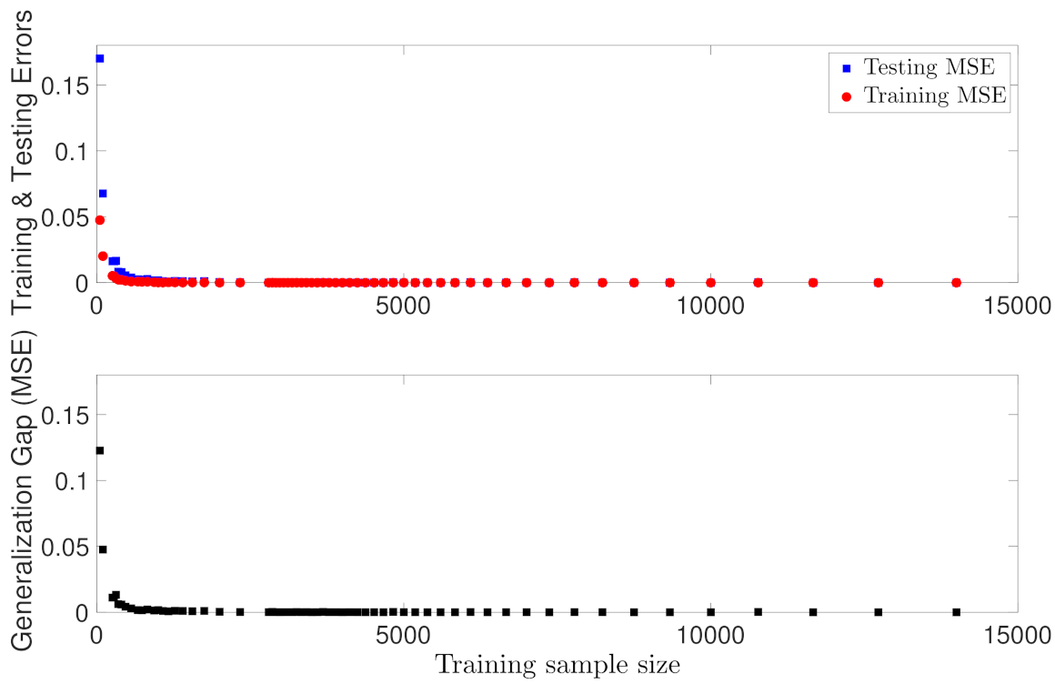
In the first case study, we trained RNN models using different data sample sizes. Specifically, we follow data generation method in [10] to initially generate a large dataset from open-loop simulation of Equation (74) under various control actions $u\in U$ and initial conditions within the stability region, i.e., $x_0\in {\mathrm{\Omega }}_{\widehat{\rho }}$. The dataset consists of 200,000 time-series data samples, and is separated into 140,000 training, 30,000 validation, and 30,000 testing samples. The RNN models are developed by gradually increasing the training sample size, and is tested using unseen data from the testing dataset. It should be noted that only the data sample size is changed in this case study, while all the other parameters such as the RNN structure (i.e., number of layers, neurons, and other hyper-parameters) and training algorithm remain the same for all RNN models. The RNN models are developed with one hidden layer of 50 neurons, and using mean squared errors (MSE) as loss function.

Figure 2 shows the variation of RNN training and testing performances with respect to the training sample size. In the top figure of Figure 2, it is observed that both the testing and training MSEs increase as training data becomes less; in the bottom figure, we show the generalization gap $\mathbb{E}\left[g_t(\mathbf{x},\mathbf{y})\right]-\frac{1}{m}{\sum }_{i=1}^m{g}_t({\mathbf{x}}_i,{\mathbf{y}}_i)$ in Equation (47), where the expected error $\mathbb{E}\left[g_t(\mathbf{x},\mathbf{y})\right]$ is approximated using the testing dataset. The trend in Figure 2 is consistent with the result in Theorem 1, which demonstrates that more training data is needed in order to obtain a lower generalization gap between expected loss and training loss. Additionally, it is noticed when the training sample size is greater than 3000, both training and testing MSEs approach zero, and no significant improvement is observed for the models using more training data. The trend in Figure 2 also follows the relation between generalization error and data sample size in Equation (47), i.e., the generalization gap $\mathbb{E}\left[g_t(\mathbf{x},\mathbf{y})\right]-\frac{1}{m}{\sum }_{i=1}^m{g}_t({\mathbf{x}}_i,{\mathbf{y}}_i)$ is roughly proportional to $\frac{1}{\sqrt{m}}$, which shows that the generalization gap initially decreases fast when the sample size m starts increasing from zero, and changes slowly when m becomes large.

5.1.2. Case Study 2: RNN Depth and Width

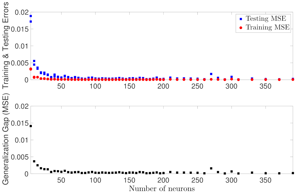
In the second case study, we train RNN models with various depths and widths. 1400 training data, 300 validation data, and 300 testing data are used for all models. We first develop RNN models by fixing the network depth as one hidden layer, and increasing the number of neurons. As shown in Figure 3, both training and testing errors decrease as the network width increases up to 250 neurons. However, as more neurons are added (i.e., 270 and 280 neurons in Figure 3), the testing MSE increases while the training MSE remains close to zero all the time, which implies that overfitting has occurred during training. As a result, the generalization gap in Figure 3 shows a similar pattern, which decreases initially and increases again when a large number of neurons are used. While theoretically the expected error of Equation (47) does not explicitly depend on the network width, the results in Figure 3 are consistent with the fact that increasing the capacity of a model by adding more layers and/or more nodes to layers can improve the network learnability, but may also lead to overfitting.

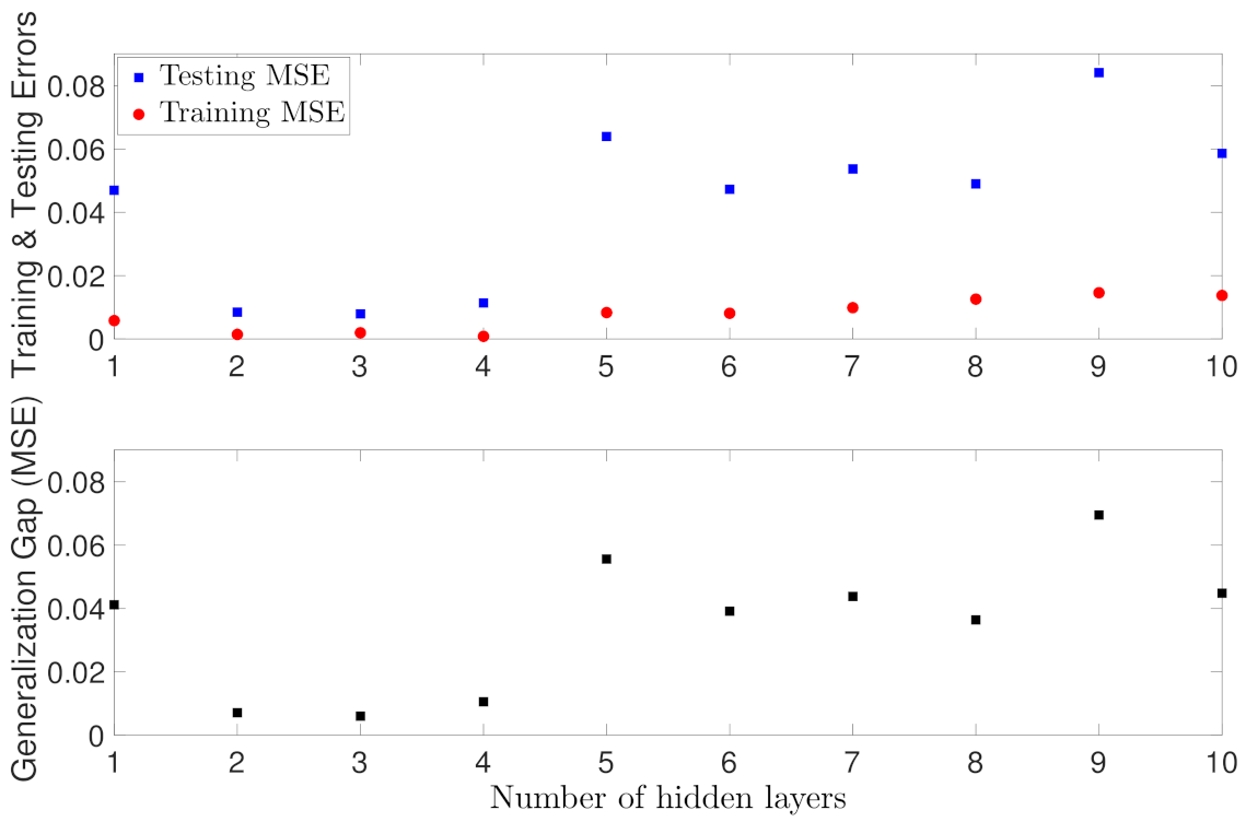
Subsequently, we train RNN models by increasing the number of layers, and fixing five neurons each layer. Figure 4 shows that the testing MSE starts at around 0.02 for one hidden layer, gradually decreases with more layers, and finally increases again as the neural network becomes deeper. Meanwhile, the training MSE remains close to zero at the beginning, yet also slightly increases as the number of hidden layers increase. From Figure 4, it is concluded that one hidden layer is not sufficient to learn the process dynamics well, and with two, three, and four layers, the RNN models achieve the best training and generalization performance among all the models. Similar to Figure 3, the increase of generalization gap in Figure 4 implies that deeper RNN models are overfitting the training data. Additionally, it is also interesting to notice that the training error slightly increases in deeper networks. While in general, the generalization performance deteriorates and the training error remains unaffected when increasing the capacity of a model, the worse training performance in Figure 4 are actually common in neural network development due to the difficulty of training deep networks. Specifically, the optimization problem of neural network training is highly non-convex, and may get stuck at some local minima as the network becomes deeper. This is noticed during the training of RNN models in Figure 4, where both the training and validation losses exhibit a sharp increase at a certain epoch and then get stuck around that point until the end of epochs. Additionally, with more hidden layers, the number of parameters to be trained grows exponentially, which could lead to a poor training performance without a careful tuning of other hyperparameters.

Remark 8.

At first glance, the generalization error trend in Figure 3 and Figure 4 seems in contrast to the results in Equation (47), which shows the generalization error bound is proportional to the complexity of RNN hypothesis class. However, it should be noted that Equation (47) only gives the upper bound for the generalization error of RNN models from the hypothesis class. It does not mean all the RNN models from the hypothesis class have a generalization error as large as its upper bound. From the error decomposition of Equation (17) showing the interplay between approximation and estimation errors, we have learned that as we enlarge the hypothesis class, the approximation error decreases, but the estimation error may increase. In this case study, by increasing the complexity of RNN hypothesis class in terms of more layers and neurons, overall the generalization performance improves; however, as the RNN models become deeper, overfitting also occurs due to a large estimation error. Therefore, in practice, we can do a grid search such as Figure 3 and Figure 4 to determine the optimal number of layers and neurons.

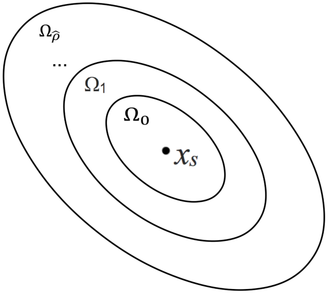
5.1.3. Case Study 3: Different Regions in ${\mathrm{\Omega }}_{\widehat{\rho }}$

As discussed in Remark 6, to meet the modeling error constraint $E_M\le \gamma \left|x\right|$, $\forall x\in {\mathrm{\Omega }}_{\widehat{\rho }}$, more data is needed as the state approaches the origin, i.e., $x\to 0$. It is equivalent to show that under the same data density for different regions within the stability region ${\mathrm{\Omega }}_{\widehat{\rho }}$, a larger constant $\gamma$ is needed to bound the modeling error $E_M\le \gamma \left|x\right|$ for the states close to the origin. Therefore, in this case study, we develop multiple RNN models for different regions inside ${\mathrm{\Omega }}_{\widehat{\rho }}$ with the same data density, and demonstrate the variation of generalization performances. Specifically, we choose 9 level sets of Lyapunov function ${\mathrm{\Omega }}_{{\rho }_i}:=\{x\in {\mathbf{R}}^n|\widehat{V}\left(x\right)\le {\rho }_i\}$, $i=0,...,8$, within ${\mathrm{\Omega }}_{\widehat{\rho }}$, with $\widehat{\rho }=368$ and ${\rho }_i=[40,88,115,138,159,177,195,213,244]$. For example, the first RNN model (model 0 with ${\rho }_0$) is developed and tested using the data within ${\mathrm{\Omega }}_{{\rho }_0}$, the second RNN model (model 1 with ${\rho }_1$) uses the data between ${\mathrm{\Omega }}_{{\rho }_0}$ and ${\mathrm{\Omega }}_{{\rho }_1}$, and so on. Figure 5 shows a schematic of the training regions considered for the CSTR of Equation (74), where $x_s$ is the steady-state, and ${\mathrm{\Omega }}_{\widehat{\rho }}$ is the stability region. The training datasets are generated for each region (i.e., elliptical annuli in Figure 5) with the same data density, where the data density is defined as the ratio of sample size to the area of each elliptical annulus. Similarly, in this case study, we use data from different regions within ${\mathrm{\Omega }}_{\widehat{\rho }}$ to build RNN models, while all the other parameters remain the same. The RNN models are developed with one hidden layer of 20 neurons, and using MSE as loss function.

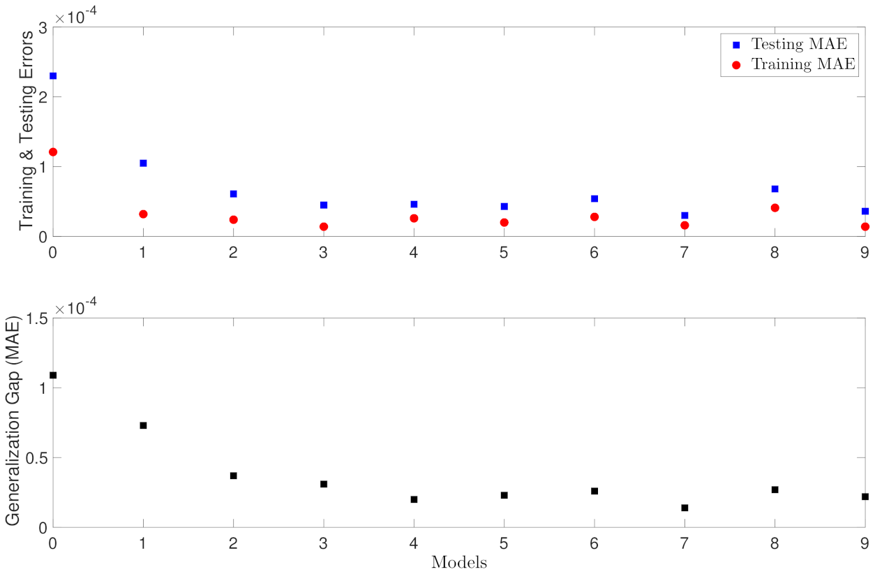
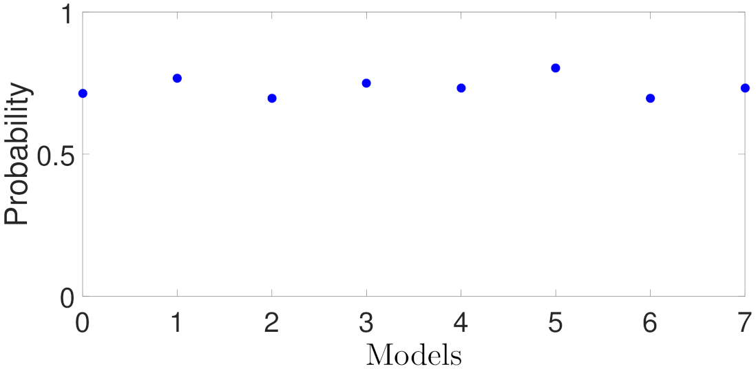
To compute the modeling error $|F(x,u)-F_{nn}(x,u)|=|\frac{dx}{dt}-\frac{d\widehat{x}}{dt}|$ where x and $\widehat{x}$ denote the true state and predicted state, respectively, we carry out prediction for one integration time step, and use finite difference method to approximate the derivatives following Equation (56). Specifically, we first calculate the training and testing mean absolute errors (MAE) and divide them by the integration time step $h_c$, i.e., $|\frac{x(t+h_c)-\widehat{x}(t+h_c)}{h_c}|$. Subsequently, to obtain an approximated value of $\gamma$ for each model, i.e., $\frac{E_M}{\left|x\right|}\le \gamma$, we divide those MAEs by the maximum value of $\left|x\right|$ in each elliptical annulus in Figure 5. Figure 6 shows the training and testing errors for the RNN models trained for different regions inside ${\mathrm{\Omega }}_{\widehat{\rho }}$. It is observed that under the same data density, the models trained for the regions close to the origin (i.e., Models 0, 1, and 2 for ${\mathrm{\Omega }}_{{\rho }_0}$, ${\mathrm{\Omega }}_{{\rho }_1}$ and ${\mathrm{\Omega }}_{{\rho }_2}$) produce larger generalization gaps. This implies a larger $\gamma$, or equivalently, more data is needed to meet the constraint $E_M\le \gamma \left|x\right|$ for x in these regions. Additionally, it is observed that the generalization gap settles at around $2\times {10}^{-5}$ for model 4 and after because those RNN models have achieved the best they can do under the current neural network training settings and data density.

5.1.4. Case Study 4: Weight Matrix Bound

From Equation (48), it is seen that the generalization gap also depends on the weight matrix bound. To evaluate the relation between generalization performance and weight matrix bound, in this case study, we train RNN models with different weight matrix bounds. Specifically, we impose an upper bound constraint for each element in the RNN weight matrices with the following values $[0.8,1.3,1.8,2.5,3.0,3.4,3.9,4.3]$.

The Frobenius norms of all the weight matrices are therefore also bounded. The training and testing errors are calculated following the approach in Case study 1, and are shown in Figure (Figure 7). It is observed that as the weight matrix bound becomes larger, the generalization gap gradually increases and settles at around $8\times {10}^{-4}$. This behavior implies that the RNN model is over-fitting when training with a large weight bound. The reason for the trend in Figure 7 is similar to that for Case study 2, which demonstrates that as the size of neural network hypothesis class becomes larger with increasing weight bounds, it is easier to find a hypothesis that fits training data well, but could also lead to large testing error (i.e., over-fitting).

5.1.5. Case Study 5: RNN Input Length

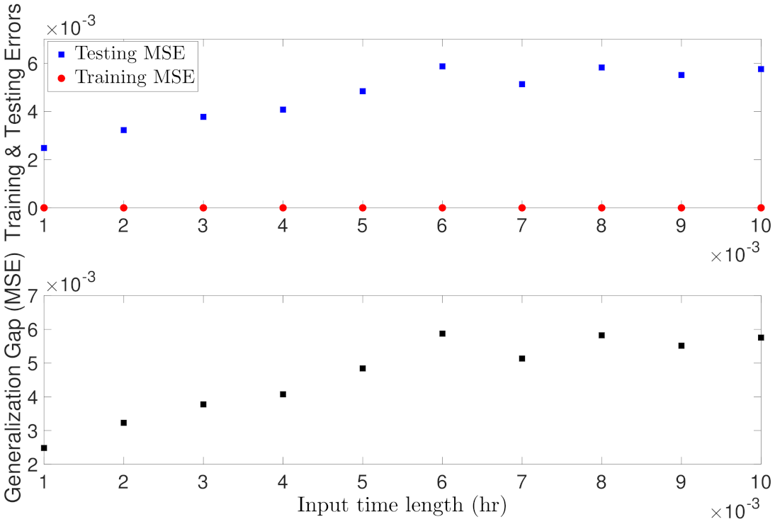
Lastly, we study the dependency of RNN generalization error on the input time length t according to Equation (47). If we unfold a vanilla RNN over time to form a multi-layer feedfoward neural network, then this relation can also be interpreted in the way that a deep feedforward neural network has a large generalization error. In this example, we train RNN models with different input time length as follows: $t={10}^{-3}\times [1,2,3,4,5,6,7,8,9,10]$ hr.

Figure 8 shows the training and testing errors for different time lengths. Specifically, as RNN input time length increases, it is seen that the training error remains at a very low level for all models, but the testing error gradually increases and finally settles at around $6\times {10}^{-3}$. It is concluded from Figure 8 that a shorter input sequence yields better generalization performance, which is consistent with the theoretical result shown in Equation (47). However, it should be noted that a shorter input sequence does not necessarily yield better prediction in the formulation of MPC because as discussed in Theorem 2, in order to predict future states for a long prediction horizon, the RNN prediction needs to be executed successively, which inevitably accumulates the error during calculations. Therefore, when used in MPC, the RNN input length should be carefully chosen to account for MPC prediction horizon and maintain a desired generalization performance simultaneously.

Remark 9.

A small training dataset was chosen in Case studies 2–5 for demonstration purposes. Specifically, it was demonstrated in Case study 1 that with more than 3000 data samples, both training and testing errors are rendered sufficiently small. Therefore, to better demonstrate the relation between RNN generalization error bound and RNN depth/width, and data time length in other case studies, we chose a small training dataset such that significant differences can be observed by varying RNN depths, widths, time sequence length. However, it is noted that in practice, the sample size and all the other factors studied in this manuscript should be carefully chosen in order to improve the RNN generalization performance.

5.2. Closed-Loop Performance Analysis

In this section, we carry out closed-loop simulations of CSTR under the LMPC of Equations (68)–(73) using the different RNN models derived from the previous case studies. Additionally, we demonstrate the probabilistic closed-loop stability properties of RNN-based LMPC through extensive closed-loop simulations for the CSTR of Equation (74) with different initial conditions.

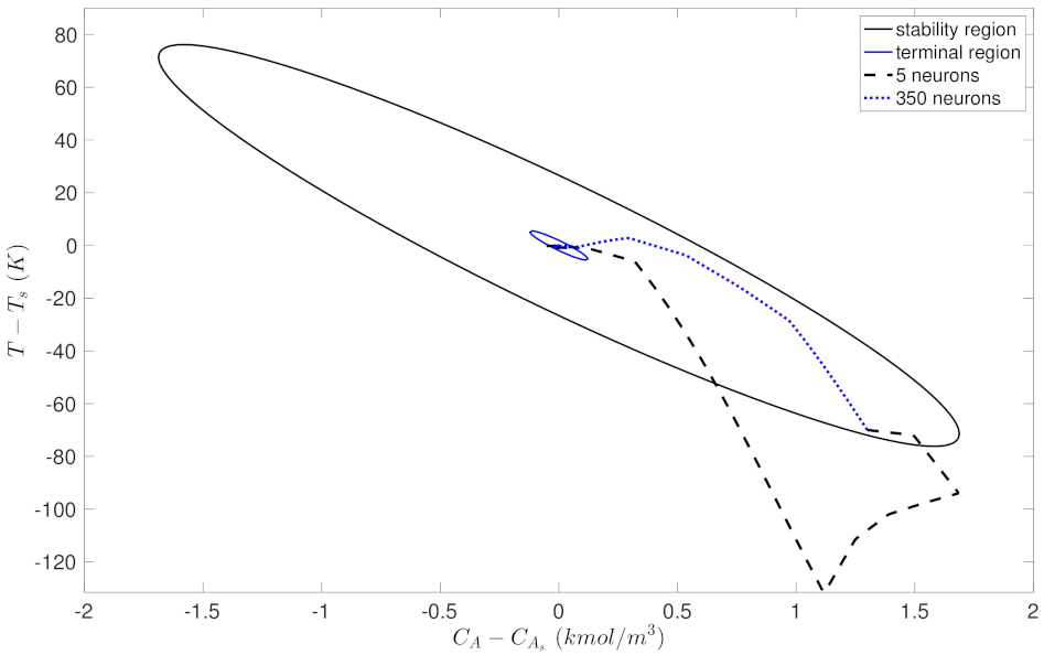
Figure 9, Figure 10, Figure 11 and Figure 12 show the simulation results using 48 different initial conditions within ${\mathrm{\Omega }}_{\widehat{\rho }}$ for a few RNN models trained in Case study 1. Specifically, we first discretize the stability region ${\mathrm{\Omega }}_{\widehat{\rho }}$ and choose 48 initial conditions $x_0\in {\mathrm{\Omega }}_{\widehat{\rho }}$ that are evenly spread within the stability region. Then, we run closed-loop simulations for all initial conditions using the following settings: (1) the whole simulation period $t_p$ is twenty sampling periods (i.e., $20\times 0.01=0.2$ hr), (2) the stability region ${\mathrm{\Omega }}_{\widehat{\rho }}$ and the terminal region ${\mathrm{\Omega }}_{{\rho }_{min}}$ are characterized as $\widehat{\rho }=368$ and ${\rho }_{min}=2$, respectively, and (3) the simulations are carried out using UCLA Hoffman 2 cluster and the optimization problem is solved using the python module of the IPOPT software package (i.e., PyIpopt). After obtaining the closed-loop profiles for each initial condition, the following policies are utilized to determine whether the closed-loop system is stable or not. Specifically, the closed-loop system is considered unstable if (1) the closed-loop state leaves the stability region ${\mathrm{\Omega }}_{\widehat{\rho }}$ at any point during the simulation, or (2) the closed-loop state remains inside ${\mathrm{\Omega }}_{\widehat{\rho }}$, but stays outside of ${\mathrm{\Omega }}_{{\rho }_{min}}$ until the end of simulation or leaves ${\mathrm{\Omega }}_{{\rho }_{min}}$ after entering for the first time.

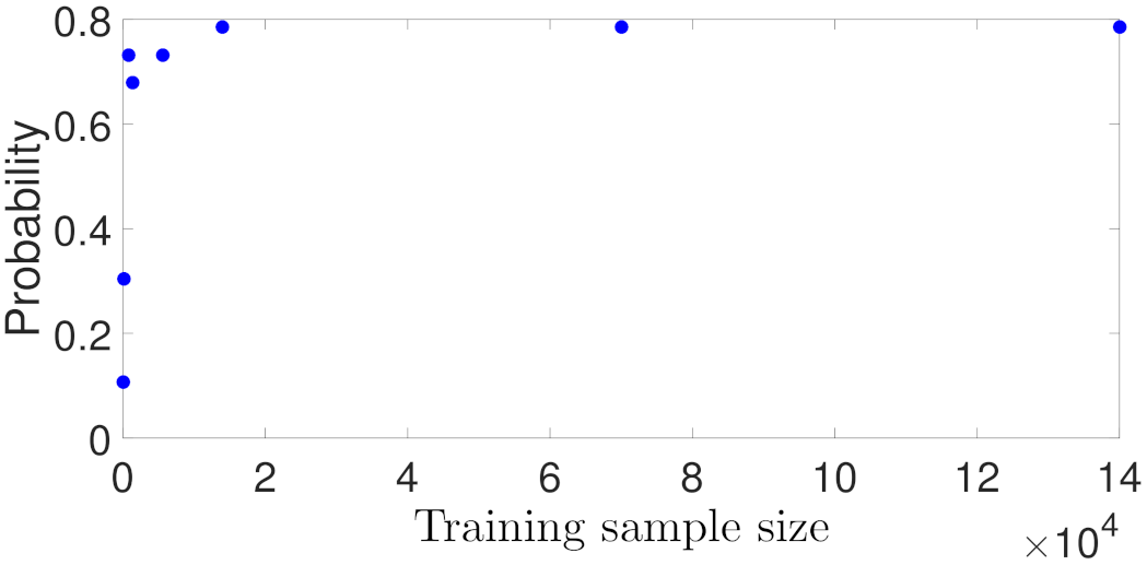
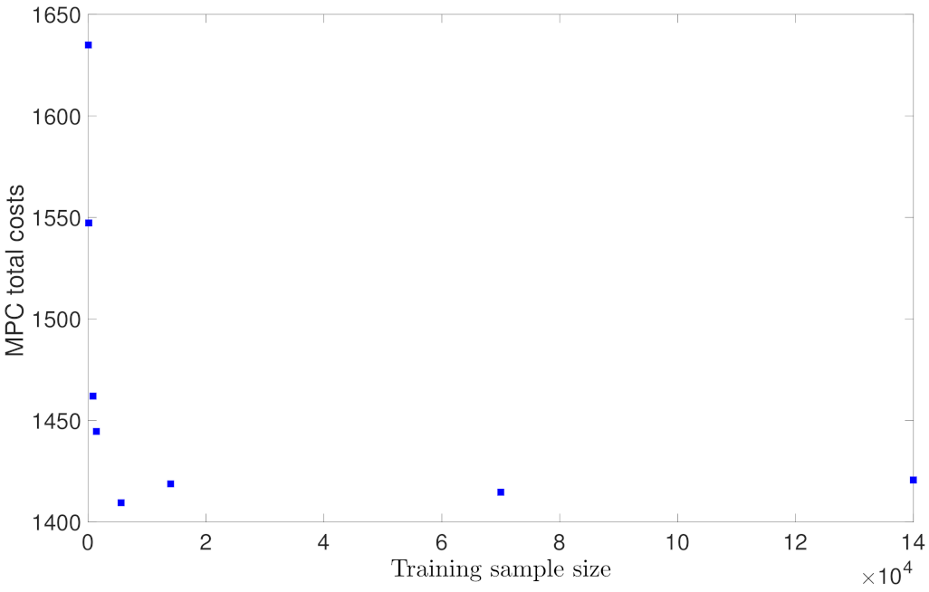
Figure 9 shows the probability of closed-loop stability calculated following the above policies. It is seen that with more training data, the probability of the CSTR of Equation (74) being stabilized at its steady-state becomes higher, and the probability settles at around 0.78 for a sufficiently large dataset. The probability results in Figure 9 for RNN models in Case study 1 are consistent with its generalization performance plot in Figure 2, which shows that the generalization error decreases with more data used for training. In addition to the calculation of the probability for closed-loop stability, we also use the MPC cost function of Equation (68) as an indicator for comparing control performance in terms of the convergence speed and energy consumption. Specifically, the MPC cost function of Equation (68) in this example is designed in the following form:

$$L_{MPC}(x,u)=x^{T}Px+u^{T}Qu$$

(76)

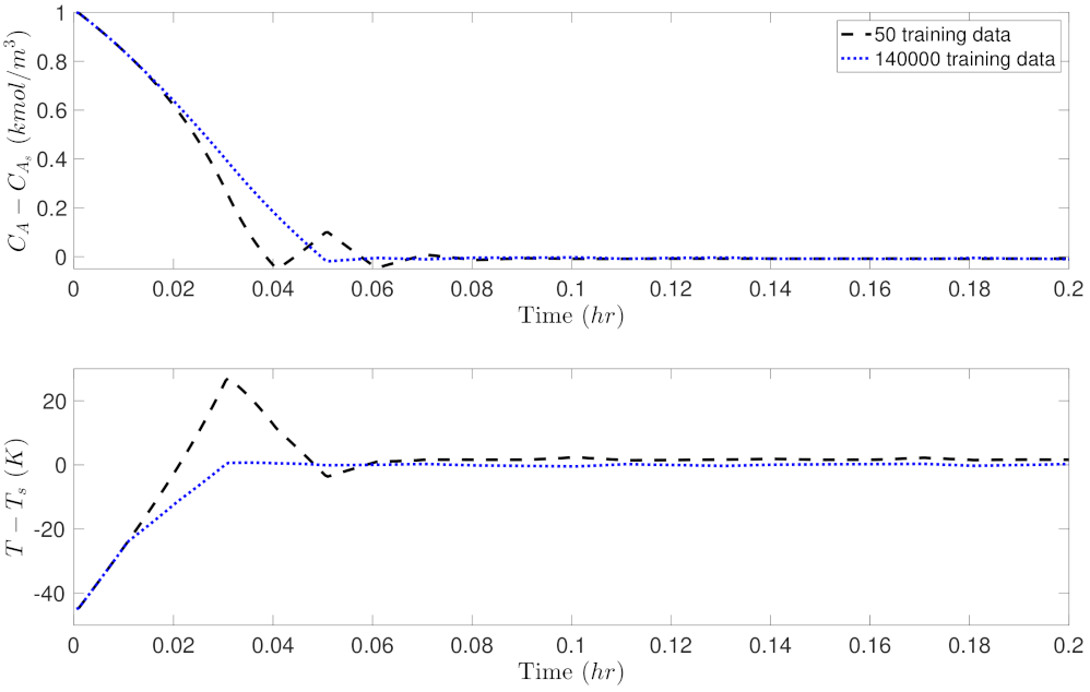
where $P=[10000;01]$ and $Q=[10;03\times {10}^{-10}]$ are chosen such that the two states and the two inputs are in the same order of magnitude, respectively. Also, in this example, we put more penalty on the states x to allow the states to be driven to the steady-state more quickly. For each RNN model, we calculate the total costs ${\int }_{t=0}^{t_p}{L}_{MPC}(x,u)dt$ over the entire simulation period $t_p=0.2$ hr, and sum up the cost values for all the trajectories initiated from 48 different initial conditions. Figure 10 shows the MPC total costs for the RNN models trained with different data sample sizes. It is demonstrated that with less training data, the MPC achieves a higher total cost, representing a slower convergence to the steady-state and/or a higher energy consumption. With a large number of training data (i.e., $\ge 6000$), the MPC total costs remain at around 1420, and no significant improvement is noticed with more data added in training. Additionally, Figure 11 and Figure 12 show the closed-loop state trajectory and state profiles for one of the initial condition out of 48 initial conditions. As shown in Figure 11, the state trajectory using the RNN model trained with 50 training data (dashed line) leaves the stability region due to poor predictions in solving the MPC optimization problem. On the contrary, the state trajectory using the RNN model with 14,000 training data (solid line) moves towards the steady-state smoothly and is ultimately bounded in the terminal set ${\mathrm{\Omega }}_{{\rho }_{min}}$. This can also be seen in the closed-loop state profiles of Figure 12, where the temperature under 50 training data shows a sharp increase at 0.03 hr.

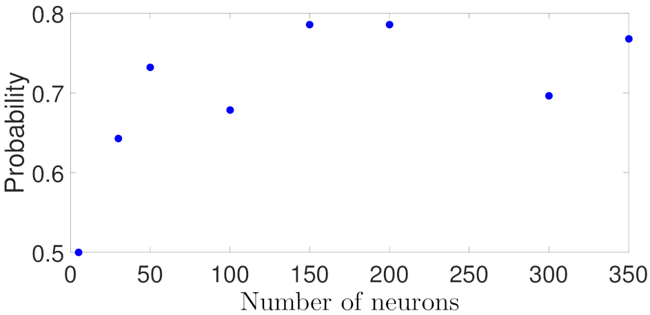
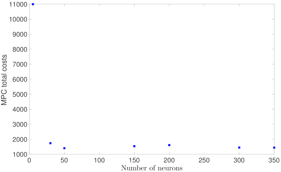
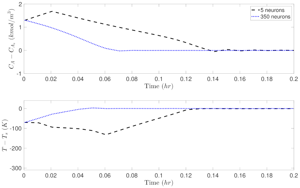
Similar to the analysis for Case study 1, Figure 13, Figure 14, Figure 15 and Figure 16 show the probability of closed-loop stability, MPC total costs, as well as the state-space trajectory and state profiles for one of the initial condition for the RNN models in Case study 2. In Figure 13, it is shown that the probability starts from 0.5, and settles at around 0.7 for wider RNN models (i.e., more neurons). Figure 14 shows the MPC total costs for different models, from which it is demonstrated that the first model with only 5 neurons has a extremely high value, and all the other models achieve a total cost around 1500. Figure 13 and Figure 14 demonstrate that all the RNN models except the first one achieve desired closed-loop performance in terms of high probability of closed-loop stability and low total costs. This is due to the low generalization error (around 0.005) for nearly all the models in Figure 3. Figure 15 shows the comparison of the closed-loop state trajectories under the two RNN models using 5 and 350 neurons, respectively, from which it is demonstrated that the model with 5 neurons (dashed line) drives the state out of the stability region, while the one with 350 neurons successfully stabilizes the system in the terminal set. The corresponding state profiles (i.e., $C_A-C_{As}$ and $T-T_s$) can be found in Figure 16.

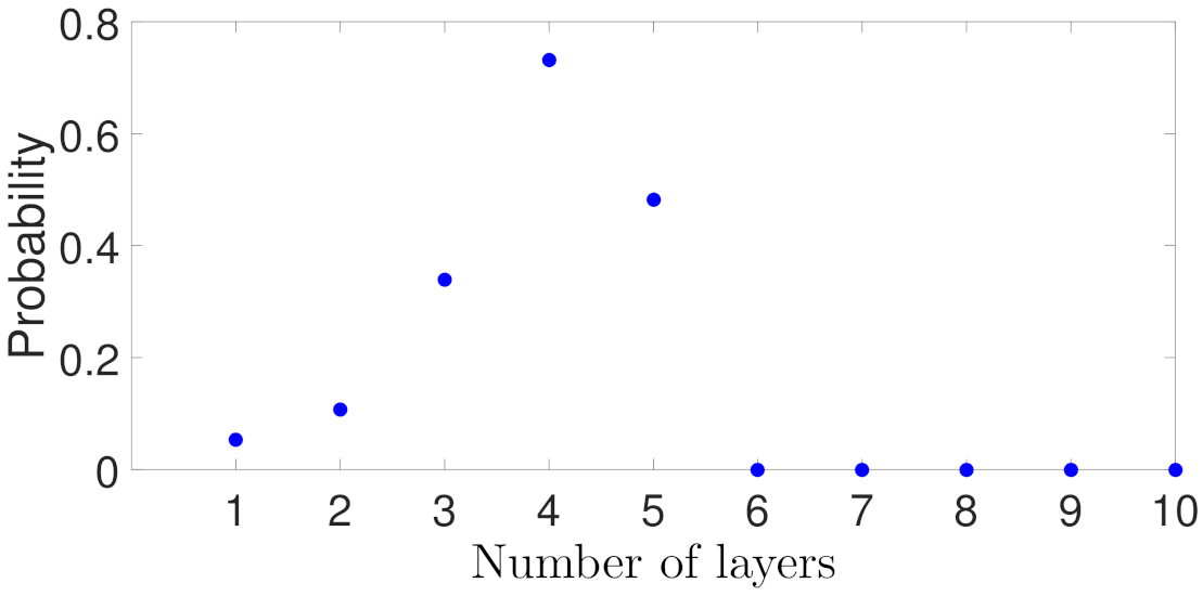
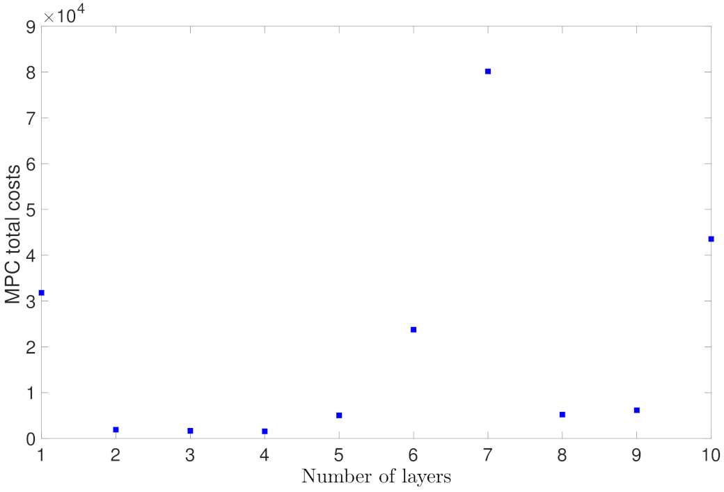
To simplify the discussion for the remaining case studies, we will show the probability plot and MPC total cost plot only. Figure 17 shows the probability of closed-loop stability with respect to different RNN depths. It is demonstrated that the probability starts close to zero for one layer, increases up to 0.7 for four layers, and then decreases to almost zero for six layer and after. This trend follows exactly the generalization error plot in Figure 4, which shows the model with two, three and four layers achieve the lowest generalization error, and the models with more than five layers show worse generalization performance due to overfitting. Comparing to the closed-loop results for the RNNs with various widths in Figure 13 and Figure 14, it is not surprising to see that the overall probability of closed-loop stability in this case study is worse because the open-loop generalization performance for the RNNs developed with different depths (Figure 4) is worse than that for the RNNs developed with different widths (Figure 3). Additionally, in Figure 18, we observe a similar pattern showing that the MPC total costs have the lowest values for two, three and four layers, and rise up for more layers.

Closed-loop simulations for Case study 3 of different regions in ${\mathrm{\Omega }}_{\widehat{\rho }}$ are not carried out in this work, since the MPC formulation of Equations (68)–(73) only uses a single RNN model for prediction. Additionally, it is demonstrated from previous case studies that a single RNN model is sufficient to capture the process dynamics in the stability region, and therefore, there is no need to use different RNN models for different regions in ${\mathrm{\Omega }}_{\widehat{\rho }}$ from the control perspective.

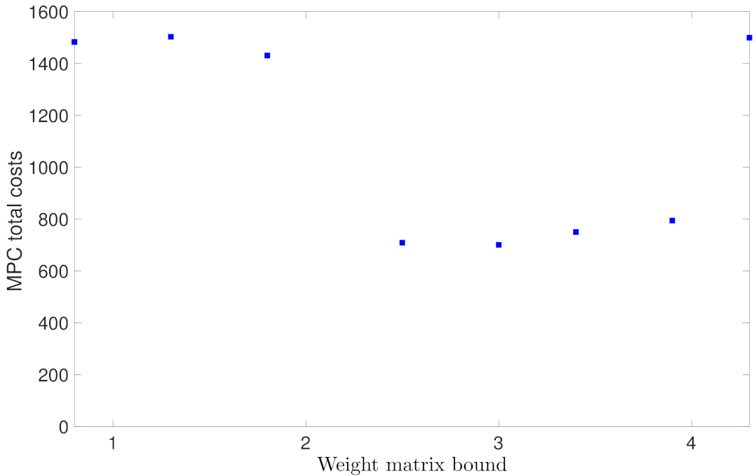
Figure 19 shows the probability of closed-loop stability for the RNN models with different weight matrix bounds in Case study 4. It is shown that all the RNN models achieve a probability up to 0.7. The high probability of closed-loop stability is expected since in the open-loop generalization error plot in Figure 7, it is shown that all the models with different weight matrix bounds have a sufficiently small generalization error around $8\times {10}^{-4}$. As a result, the MPC total costs in Figure 20 are stable around 1000 for all models.

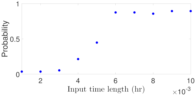
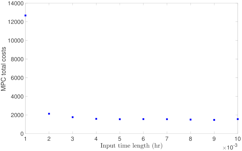
Lastly, Figure 21 and Figure 22 show the closed-loop simulation results for Case study 5. As shown in Figure 21, the probability of closed-loop stability increases as the RNN input time length increases, and settles at around 0.9 for input time length greater than $6\times {10}^{-3}$ hr. This seems inconsistent with the generalization performance of Figure 8 which shows the generalization error increases for longer input sequences at first glance. However, as we have discussed earlier, a low open-loop generalization error for short input sequences does not guarantee a desired closed-loop performance under MPC. Specifically, with shorter input sequences, the RNN prediction needs to be executed successively in each MPC iteration to predict all the future states within the prediction horizon. For example, in order to predict one sampling time $\Delta ={10}^{-2}$ hr, the first RNN model with $1\times {10}^{-3}$ input length in Figure 21 needs to run 10 times, and each time uses the previous predicted state as the initial state. The error accumulates during the calculation, which ultimately leads to poorer closed-loop performance. Therefore, for RNN models used in MPC, the input time length should be chosen carefully accounting for the system sampling time and MPC prediction horizon. Additionally, Figure 22 shows the MPC total costs with respect to different RNN input time lengths. It is seen that the first RNN model achieves the worst cost value, and all the other models have similar cost values around 2000. Through the closed-loop simulation of all the case studies investigated in the previous section, we demonstrate that the closed-loop performance is consistent with the open-loop generalization performance in the way that lower generalization errors typically leads to higher probability of closed-loop stability and lower MPC total costs. Therefore, the generalization error bound proposed in this work provides an efficient method for choosing neural network structure and data sample size to meet the closed-loop stability requirements.

Remark 10.

The RNN models are trained offline, and the RNN-based MPC is solved in real time with new state measurements available at each sampling time. The averaged computation time for solving RNN-based MPC per sampling step is around 10 s, which is less than one sampling period $\Delta =0.01hr=36s$ in this example. Therefore, the RNN-based MPC scheme can be implemented in real time without any computational issues.

6. Conclusions

In this work, we developed a generalization probabilistic error bound for RNN models by taking advantage of the Rademacher complexity method for vector-valued functions. The RNN models were incorporated in the design of MPC, and probabilistic closed-loop stability properties were derived based on the RNN generalization error bounds. A number of case studies were simulated using a nonlinear chemical reactor example to demonstrate the impact of training sample size, the number of neurons and layers, regions where the data was generated, and input time length on the RNN generalization performance. Closed-loop simulation were carried out to further demonstrate the probabilistic closed-loop stability properties derived by the RNN-based LMPC.

References

- Cozad, A.; Sahinidis, N.V.; Miller, D.C. A combined first-principles and data-driven approach to model building. Comput. Chem. Eng. 2015, 73, 116–127. [Google Scholar] [CrossRef]
- Wilson, Z.T.; Sahinidis, N.V. The ALAMO approach to machine learning. Comput. Chem. Eng. 2017, 106, 785–795. [Google Scholar] [CrossRef] [Green Version]
- Ali, J.M.; Hussain, M.A.; Tade, M.O.; Zhang, J. Artificial Intelligence techniques applied as estimator in chemical process systems–A literature survey. Expert Syst. Appl. 2015, 42, 5915–5931. [Google Scholar]
- Han, H.; Wu, X.; Qiao, J. Real-time model predictive control using a self-organizing neural network. IEEE Trans. Neural Netw. Learn. Syst. 2013, 24, 1425–1436. [Google Scholar] [PubMed]
- Wang, T.; Gao, H.; Qiu, J. A combined adaptive neural network and nonlinear model predictive control for multirate networked industrial process control. IEEE Trans. Neural Netw. Learn. Syst. 2016, 27, 416–425. [Google Scholar] [CrossRef] [PubMed]
- Wang, Y. A new concept using LSTM Neural Networks for dynamic system identification. In Proceedings of the American Control Conference 2017, Seattle, WA, USA, 24–26 May 2017; pp. 5324–5329. [Google Scholar]
- Wong, W.; Chee, E.; Li, J.; Wang, X. Recurrent Neural Network-Based Model Predictive Control for Continuous Pharmaceutical Manufacturing. Mathematics 2018, 6, 242. [Google Scholar] [CrossRef] [Green Version]
- Shahnazari, H.; Mhaskar, P.; House, J.M.; Salsbury, T.I. Modeling and fault diagnosis design for HVAC systems using recurrent neural networks. Comput. Chem. Eng. 2019, 126, 189–203. [Google Scholar] [CrossRef]
- Wu, Z.; Tran, A.; Rincon, D.; Christofides, P.D. Machine Learning-Based Predictive Control of Nonlinear Processes. Part I: Theory. AIChE J. 2019, 65, e16729. [Google Scholar] [CrossRef]
- Wu, Z.; Tran, A.; Rincon, D.; Christofides, P.D. Machine Learning-Based Predictive Control of Nonlinear Processes. Part II: Computational Implementation. AIChE J. 2019, 65, e16734. [Google Scholar] [CrossRef]
- Pan, Y.; Wang, J. Nonlinear model predictive control using a recurrent neural network. In Proceedings of the IEEE International Joint Conference on Neural Networks 2008, Hong Kong, China, 1–8 June 2008; pp. 2296–2301. [Google Scholar]
- Pan, Y.; Wang, J. Model predictive control of unknown nonlinear dynamical systems based on recurrent neural networks. IEEE Trans. Ind. Electron. 2011, 59, 3089–3101. [Google Scholar] [CrossRef]
- Xu, J.; Li, C.; He, X.; Huang, T. Recurrent neural network for solving model predictive control problem in application of four-tank benchmark. Neurocomputing 2016, 190, 172–178. [Google Scholar] [CrossRef]
- Hoskins, J.; Himmelblau, D. Process control via artificial neural networks and reinforcement learning. Comput. Chem. Eng. 1992, 16, 241–251. [Google Scholar] [CrossRef]
- Vepa, R. A review of techniques for machine learning of real-time control strategies. Intell. Syst. Eng. 1993, 2, 77–90. [Google Scholar] [CrossRef]
- Hussain, M. Review of the applications of neural networks in chemical process control—Simulation and online implementation. Artif. Intell. Eng. 1999, 13, 55–68. [Google Scholar] [CrossRef]
- Hewing, L.; Wabersich, K.; Menner, M.; Zeilinger, M. Learning-based model predictive control: Toward safe learning in control. Annu. Rev. Control Robot. Auton. Syst. 2020, 3, 269–296. [Google Scholar] [CrossRef]
- Venkatasubramanian, V. The promise of artificial intelligence in chemical engineering: Is it here, finally? AIChE J. 2019, 65, 466–478. [Google Scholar] [CrossRef]
- Mittal, M.; Gallieri, M.; Quaglino, A.; Salehian, S.; Koutník, J. Neural lyapunov model predictive control. arXiv 2020, arXiv:2002.10451. [Google Scholar]
- Limon, D.; Calliess, J.; Maciejowski, J. Learning-based nonlinear model predictive control. IFAC-PapersOnLine 2017, 50, 7769–7776. [Google Scholar] [CrossRef]
- Aswani, A.; Gonzalez, H.; Sastry, S.; Tomlin, C. Provably safe and robust learning-based model predictive control. Automatica 2013, 49, 1216–1226. [Google Scholar] [CrossRef] [Green Version]
- Valiant, L.G. A theory of the learnable. Commun. ACM 1984, 27, 1134–1142. [Google Scholar] [CrossRef] [Green Version]
- Lygeros, J.; Margellos, K.; Prandini, M. Compression learning for chance constrained stochastic MPC. IFAC-PapersOnLine 2015, 48, 286–293. [Google Scholar] [CrossRef]
- Zhou, Y.; Li, D.; Spanos, C. Learning optimization friendly comfort model for HVAC model predictive control. In Proceedings of the 2015 IEEE International Conference on Data Mining Workshop (ICDMW), Atlantic City, NJ, USA, 14–17 November 2015; pp. 430–439. [Google Scholar]
- Bartlett, P.; Foster, D.J.; Telgarsky, M. Spectrally-normalized margin bounds for neural networks. arXiv 2017, arXiv:1706.08498. [Google Scholar]
- Zhang, Y.; Lee, J.; Wainwright, M.; Jordan, M.I. On the learnability of fully-connected neural networks. In Proceedings of the Artificial Intelligence and Statistics PMLR 2017, Fort Lauderdale, FL, USA, 20–22 April 2017; pp. 83–91. [Google Scholar]
- Golowich, N.; Rakhlin, A.; Shamir, O. Size-independent sample complexity of neural networks. In Proceedings of the Conference On Learning Theory PMLR 2018, Stockholm, Sweden, 5–9 July 2018; pp. 297–299. [Google Scholar]
- Cao, Y.; Gu, Q. Tight sample complexity of learning one-hidden-layer convolutional neural networks. arXiv 2019, arXiv:1911.05059. [Google Scholar]
- Chen, M.; Li, X.; Zhao, T. On generalization bounds of a family of recurrent neural networks. arXiv 2019, arXiv:1910.12947. [Google Scholar]
- Cao, Y.; Gu, Q. Generalization bounds of stochastic gradient descent for wide and deep neural networks. arXiv 2019, arXiv:1905.13210. [Google Scholar]
- Zou, D.; Gu, Q. An improved analysis of training over-parameterized deep neural networks. arXiv 2019, arXiv:1906.04688. [Google Scholar]
- Akpinar, N.; Kratzwald, B.; Feuerriegel, S. Sample complexity bounds for recurrent neural networks with application to combinatorial graph problems. arXiv 2019, arXiv:1901.10289. [Google Scholar]
- Reid, M. Generalization bounds. In Encyclopedia of Machine Learning; Springer: Boston, MA, USA, 2010; pp. 447–454. [Google Scholar] [CrossRef]
- Hanson, J.; Raginsky, M.; Sontag, E. Learning Recurrent Neural Net Models of Nonlinear Systems. arXiv 2020, arXiv:2011.09573. [Google Scholar]
- Sammut, C.; Webb, G.I. Encyclopedia of Machine Learning; Springer Science & Business Media: Berlin/Heidelberg, Germany, 2011. [Google Scholar]
- Maurer, A. A vector-contraction inequality for rademacher complexities. In Lecture Notes in Computer Science, Proceedings of the International Conference on Algorithmic Learning Theory, Bari, Italy, 19–21 October 2016; Springer: Berlin/Heidelberg, Germany, 2016; pp. 3–17. [Google Scholar]
- Mohri, M.; Rostamizadeh, A.; Talwalkar, A. Foundations of Machine Learning; MIT Press: Cambridge, MA, USA, 2018. [Google Scholar]
- Ledoux, M.; Talagrand, M. Probability in Banach Spaces: Isoperimetry and Processes; Springer Science & Business Media: Berlin/Heidelberg, Germany, 2013. [Google Scholar]
- Wu, Z.; Rincon, D.; Christofides, P.D. Process structure-based recurrent neural network modeling for model predictive control of nonlinear processes. J. Process Control 2020, 89, 74–84. [Google Scholar] [CrossRef]
- Keras. Available online: https://keras.io (accessed on 1 August 2015).
- Wächter, A.; Biegler, L.T. On the implementation of an interior-point filter line-search algorithm for large-scale nonlinear programming. Math. Program. 2006, 106, 25–57. [Google Scholar] [CrossRef]
Figure 1.
Recurrent neural network structure.
Figure 2.
RNN generalization performance vs. training sample size.
Figure 3.
RNN generalization performance vs. RNN width (One hidden layer with increasing number of neurons).
Figure 4.
RNN generalization performance vs. RNN depth (Increasing the number of hidden layers and fixing 5 neurons for each layer).
Figure 5.
Schematic of different regions inside .
Figure 6.
RNN generalization performance vs. different regions in .
Figure 7.
RNN generalization performance vs. weight matrix bound.
Figure 8.
RNN generalization performance vs. input time length.
Figure 9.
Probability of closed-loop stability vs. training sample sizes.
Figure 10.
MPC total costs vs. training sample size.
Figure 11.
Closed-loop state trajectory under LMPC using two RNN models trained with different data sample sizes.
Figure 12.
Closed-loop state profiles under LMPC using two RNN models trained with different data sample sizes.
Figure 13.
Probability of closed-loop stability vs. RNN width.
Figure 14.
MPC total costs vs. RNN width.
Figure 15.
Closed-loop state trajectory under LMPC using two RNN models trained with different widths.
Figure 16.
Closed-loop state profiles under LMPC using two RNN models trained with different widths.
Figure 17.
Probability of closed-loop stability vs. RNN depth.
Figure 18.
MPC total costs vs. RNN depth.
Figure 19.
Probability of closed-loop stability vs. weight matrix bound.
Figure 20.
MPC total costs vs. weight matrix bound.
Figure 21.
Probability of closed-loop stability vs. input time length.
Figure 22.
MPC total costs vs. input time length.
Publisher’s Note: MDPI stays neutral with regard to jurisdictional claims in published maps and institutional affiliations. |
© 2021 by the authors. Licensee MDPI, Basel, Switzerland. This article is an open access article distributed under the terms and conditions of the Creative Commons Attribution (CC BY) license (https://creativecommons.org/licenses/by/4.0/).
Share and Cite
MDPI and ACS Style
Wu, Z.; Rincon, D.; Gu, Q.; Christofides, P.D. Statistical Machine Learning in Model Predictive Control of Nonlinear Processes. Mathematics 2021, 9, 1912. https://0-doi-org.brum.beds.ac.uk/10.3390/math9161912
AMA Style
Wu Z, Rincon D, Gu Q, Christofides PD. Statistical Machine Learning in Model Predictive Control of Nonlinear Processes. Mathematics. 2021; 9(16):1912. https://0-doi-org.brum.beds.ac.uk/10.3390/math9161912
Chicago/Turabian StyleWu, Zhe, David Rincon, Quanquan Gu, and Panagiotis D. Christofides. 2021. "Statistical Machine Learning in Model Predictive Control of Nonlinear Processes" Mathematics 9, no. 16: 1912. https://0-doi-org.brum.beds.ac.uk/10.3390/math9161912
Note that from the first issue of 2016, this journal uses article numbers instead of page numbers. See further details here.