Hamy Mean Operators Based on Complex q-Rung Orthopair Fuzzy Setting and Their Application in Multi-Attribute Decision Making

Abstract

To determine the connection among any amounts of attributes, the Hamy mean (HM) operator is one of the more broad, flexible, and dominant principles used to operate problematic and inconsistent information in actual life dilemmas. Furthermore, for the option to viably portray more complicated fuzzy vulnerability data, the idea of complex q-rung orthopair fuzzy sets can powerfully change the scope of sign of choice data by changing a boundary q, dependent on the distinctive wavering degree from the leaders, where $\zeta \ge 1$, so they outperform the conventional complex intuitionistic and complex Pythagorean fuzzy sets. In genuine dynamic issues, there is frequently a communication problem between credits. The goal of this study is to initiate the HM operators based on the flexible complex q-rung orthopair fuzzy (Cq-ROF) setting, called the Cq-ROF Hamy mean (Cq-ROFHM) operator and the Cq-ROF weighted Hamy mean (Cq-ROFWHM) operator, and some of their desirable properties are investigated in detail. A multi-attribute decision-making (MADM) dilemma for investigating decision-making problems under the Cq-ROF setting is explored with certain examples. Finally, a down-to-earth model for big business asset-arranging framework determination is provided to check the created approach and to exhibit its reasonableness and adequacy. The exploratory outcomes show that the clever MADM strategy is better than the current MADM techniques for managing MADM issues.

1. Introduction

MADM is the fundamental significance of the decision-making (DM) science whose goal is to perceive the best option(s) from the set of likely ones. In genuine DM, an individual needs to assess the given alternatives by various classes, such as single, span, and so forth, of assessment purposes. Be that as it may, in different capricious conditions, it is generally trying for the individual to deliver their decisions as a fresh number. For this, the principle of intuitionistic fuzzy set (IFS), initiated by Atanassov [1], is used, by putting the falsity grade (FG) in the principle of fuzzy set [2]. The rule of IFS is extensively modified compared to the rule of FS, such that the sum of the duplet cannot exceed the unit interval. When the proposal of IFS was developed, it gained broad attention, and certain researchers have employed it in separate regions. For example, Liu et al. [3] initiated the hybrid approach based on variable weight under IFSs, Garg and Rani [4] elaborated the certain types of measures by using a right-angle triangle under the IFSs, and Xue and Deng [5] proposed the granular uncertainty measures based on IFSs. Thao [6] discovered certain entropy and divergent measures based on IFSs, Rahman et al. [7] explored the generalized Einstein operators under the IFSs, Kar et al. [8] presented the trapezoidal intuitionistic type-2 fuzzy setting and their application in decision-making, Bhattacharyee et al. [9] utilized the optimization theory in the field of IFSs, and Ejegwa and Onyeke [10] elaborated the statistical review of certain types of measures by using IFSs.

In some situations, the theory of IFS has failed. For instance, when a person obtains $0.6$ for the truth grade (TG) and $0.5$ for the FG, the theory of IFS is not able to cope with it, i.e., $0.6+0.5=1.1>1$, and therefore the rule of IFS has been neglected. Similarly, there are certain problems in genuine life concerns where the principle of IFS has been neglected. For this, Yager [11] improved the rule of IFS to initiate the principle of Pythagorean FS (PFS), with a rule stating that the sum of the squares of the duplet cannot exceed [0, 1]. Moreover, Garg [12] comprehensively reviewed the various approaches for solving the decision-making approach under the PFS environment. Bakioglu and Atahan [13] introduced the TOPSIS, AHP, and VIKOR methods for PFSs, Sarkar and Biswas [14] introduced the AHP-TOPSIS method for PFSs, Naeem et al. [15] initiated the Pythagorean m-polar fuzzy sets and their applications, Deb and Roy [16] developed the network information by using software under PFSs, Zulqarnain et al. [17] elaborated the aggregation operators for PFSs, and Satirad et al. [18] presented the UP-algebra in the environment of PFSs.

Researchers have employed the principle of PFS in distinct regions based on their powerful structure. However, in various circumstances, the principle of PFS is neglected, for example, if an individual provided information in the shape of $\left(0.9, 0.8\right)$ for the truth grade (TG) and FG, such that ${0.9}^2+{0.8}^2=0.81+0.64=1.45>1$, then the rule of PFS has been neglected. Similarly, as mentioned above, there are certain problems in genuine life concerns where the principle of PFS has been neglected. Yager [19] improved the rule of PFS to initiate the principle of q-rung orthopair FS (q-ROFS), with a rule that states that the sum of the q-powers of the duplet cannot exceed [0, 1]. IFS and PFS are special cases of the q-ROFS used to effectively determine the consistency of the initiated operators. When the proposal of q-ROFS was developed, it gained broad attention from various researchers, who have employed it in separate regions. For example, Garg [20] initiated possibility degree measures for using q-ROFSs, Liu et al. [21] presented the bidirectional projection under q-ROFSs, Garg [22] proposed the exponential operations under the q-ROFSs, Khan et al. [23] developed the knowledge measures under q-ROFSs, and Jan et al. [24] introduced the generalized dice measures for q-ROFSs.

In everyday life, vulnerability and ambiguity, which are available in the information, happen simultaneously with changes to the stage (periodicity) of the information. Subsequently, the current speculations are inadequate to consider this data, and consequently, there is a data misfortune during the cycle. To defeat it, the theory of complex IFS (CIFS), initiated by Alkouri and Salleh [25], is used, by putting the FG in the principle of complex FS (CFS) [26]. The rule of CIFS is extensively modified compared to the rule of CFS, such that the sum of the real and unreal parts of the duplet cannot exceed [0, 1]. The proposal of CIFS has received attention from various researchers, who have employed it in separate regions. For example, Garg and Rani [27] explored the aggregation operators for complex interval valued IFSs, Rani and Garg [28] proposed certain measures for CIFSs, Garg and Rani [29] introduced the robust measures for CIFSs, and Garg and Rani [30] initiated the aggregation operators for CIFSs. Researchers have employed the principle of CIFSs in distinct regions based on its powerful structure. However, in various circumstances, the principle of CIFS is neglected, for example, if an individual provided information in the shape of $\left(0.6e^{i2\pi \left(0.6\right)},0.5e^{i2\pi \left(0.5\right)}\right)$ for the TG and FG, such that $0.6+0.5=1.1>1, 0.6+0.5=1.1>1$, then the rule of CIFS has been neglected. There are also certain problems in genuine life concerns in which the principle of CIFS has been neglected. For this, Ullah et al. [31] improved the rule of CIFS to initiate the principle of complex PFS (CPFS), with a rule that states that the sum of the squares of the real and unreal parts of the duplet cannot exceed [0, 1]. CIFS is a special case of the CPFS used to effectively determine the consistency of the initiated operators. CPFS gained broad attention from researchers, whohave employed it in separate regions.

The Cq-ROFSs was first evolved by Liu et al. [32,33], which is the speculation of CIFS and CPFS. In Cq-ROFSs, the amount of the q-th force of the genuine part (additionally for the imaginary part) of the participation and the q-th force of the genuine part (likewise for the imaginary part) of the non-enrollment is not multiple. The Cq-ROFSs can manage circumstances which cannot be managed by CIFS and CPFS. For instance, the trait esteem is $\left(0.9e^{i2\pi \left(0.9\right)},0.8e^{i2\pi \left(0.8\right)}\right)$ in the evaluation of the employee’s performance. Obviously, ${0.9}^2+{0.8}^2=0.81+0.64=1.45>1,{0.9}^2+{0.8}^2=0.81+0.64=1.45>1$. However, if $\zeta =5$, then ${0.9}^5+{0.8}^5=0.91817<1$. Consequently, we can utilize Cq-ROFSs to portray information that cannot be managed by CIFS and CPFS. In addition, CIFS and CPFS are for the most part extraordinary instances of the Cq-ROFSs. Some investigations have been carried out, and numerous researchers have used Cq-ROFSs in the environment of various areas. For example, Mahmood and Ali [34] initiated the certain entropy and TOPSIS method for Cq-ROFSs, Ali and Mahmood [35] initiated Maclaurin symmetric mean operators for Cq-ROFSs, and Mahmood and Ali [36] explored the aggregation operators under Cq-ROFSs.

To find the relation between any number of attributes, the HM operator is one of the more broad, flexible, and dominant principles used to operate problematic and inconsistent information in actual life dilemmas, and certain researchers have implemented it in the environment of various areas. For example, Wu et al. [37] initiated the HM operators for interval valued IFSs, Li et al. [38] proposed the Dombi HM operators for IFSs, Wu et al. [39] developed the Dombi HM operators for interval valued IFSs, Liang [40] also initiated the HM operators for IFSs, Li et al. [41] explored the HM operators for PFSs, and Wang et al. [42] investigated the HM operators under the q-ROFSs. However, to date, no one has utilized the principle of HM operators in the environment of CIFS, CPFS, and Cq-ROFSs. Based on the above analysis, we develop certain operators based on Cq-ROFSs. The main aims and contributions of this paper are:

(1)

To initiate the HM operators based on the flexible Cq-ROF setting, called the Cq-ROFHM operator and the Cq-ROFWHM operator.

(2)

By using different values of parameters, certain special cases of the investigated operators are also utilized and justified with the help of numerous examples.

(3)

A down-to-earth model for big business asset-arranging framework determination is provided to check the created approach and to exhibit its reasonableness and adequacy.

(4)

The exploratory outcomes show that the clever MADM strategy outperforms the current MADM techniques for managing MADM issues.

The rest of the paper is structured as follows: A few fundamentals identified with CPFS are audited in Section 2. In Section 3, the Cq-ROFHM and Cq-ROFHM administrators are presented, and their elements are provided. In Section 4, an original MADM technique is presented. In Section 5, a few models are provided to affirm the original technique and a relative investigation is performed with current strategies. Section 6 concludes the paper.

2. Preliminaries

Various researchers have employed the principle of CPFS in distinct regions based on its powerful structure. However, in some circumstances, the principle of CPFS is neglected; for example, if an individual provided information in the shape of $\left(0.9e^{i2\pi \left(0.9\right)},0.8e^{i2\pi \left(0.8\right)}\right)$ for the TG and FG, such that ${0.9}^2+{0.8}^2=0.81+0.64=1.45>1,{0.9}^2+{0.8}^2=0.81+0.64=1.45>1$, then the rule of CPFS has been neglected. For this, Liu et al. [32,33] initiated the theory of CQROFS. CIFS and CPFS are special cases of the Cq-ROFS used to effectively determine the consistency of the initiated operators. The goal of this study is to recall certain prevailing principles, such as Cq-ROFSs and their algebraic laws with HM operators. Throughout this study, the TG, FG, and fixed set are expressed by ${\mu }_E^{\prime }\left(\psi \right),{\xi }_E^{\prime }\left(\psi \right)$ and $X$.

Definition 1.

Reference [32]: A Cq-ROFS is elaborated by:

$$E=\left\{\left(\upsilon ,{\mu }_E^{\prime }\left(\upsilon \right),{\xi }_E^{\prime }\left(\upsilon \right)\right):\upsilon \in X\right\}$$

with the rules:$0\preccurlyeq {\mu }_E^{\zeta }\left(\upsilon \right)+{\xi }_E^{\zeta }\left(\upsilon \right),{\mathsf{\phi }}_{{\mu }_E}^{\zeta }\left(\upsilon \right)+{\mathsf{\phi }}_{{\xi }_E}^{\zeta }\left(\upsilon \right)\preccurlyeq 1$. The Cq-ROFN is expressed by$\mathcal{A}=\left({\mu }_E^{\prime },{\xi }_E^{\prime }\right)=\left({\mu }_E\left(\upsilon \right).e^{\mathrm{ἷ}2{\mathsf{\pi }\mathsf{\phi }}_{{\mu }_E}\left(\upsilon \right)},{\xi }_E\left(\upsilon \right).e^{\mathrm{ἷ}2{\mathsf{\pi }\mathsf{\phi }}_{{\xi }_E}\left(\upsilon \right)}\right)$.

Definition 2.

Reference [33]: Let$\mathcal{A}=\left(\mu .e^{\mathrm{ἷ}2{\mathsf{\pi }\mathsf{\phi }}_{\mu }\left(\upsilon \right)},\xi .e^{\mathrm{ἷ}2{\mathsf{\pi }\mathsf{\phi }}_{\xi }\left(\upsilon \right)}\right),{\mathcal{A}}_1=\left({\mu }_1\left(\upsilon \right).e^{\mathrm{ἷ}2{\mathsf{\pi }\mathsf{\phi }}_{{\mu }_1}\left(\upsilon \right)},{\xi }_1\left(\upsilon \right).e^{\mathrm{ἷ}2{\mathsf{\pi }\mathsf{\phi }}_{{\xi }_1}\left(\upsilon \right)}\right),$and${\mathcal{A}}_2=\left({\mu }_2\left(\upsilon \right).e^{\mathrm{ἷ}2{\mathsf{\pi }\mathsf{\phi }}_{{\mu }_2}\left(\upsilon \right)},{\xi }_2\left(\upsilon \right).e^{\mathrm{ἷ}2{\mathsf{\pi }\mathsf{\phi }}_{{\xi }_2}\left(\upsilon \right)}\right)$be any three Cq-ROFNs, and$\mathsf{\gamma }>0$be the real number, then:

(1) 

${\mathcal{A}}^c=\left(\xi .e^{\mathrm{ἷ}2\pi {\phi }_{\xi }\left(\upsilon \right)},\mu .e^{\mathrm{ἷ}2\pi {\phi }_{\mu }\left(\upsilon \right)}\right)$;

(2) 

${\mathcal{A}}_1\vee {\mathcal{A}}_2=\left(max\left({\mu }_1,{\mu }_2\right).e^{\mathrm{ἷ}2\pi .max\left({\phi }_{{\mu }_1}\left(\psi \right),{\phi }_{{\mu }_2}\left(\psi \right)\right)},min\left({\xi }_1,{\xi }_2\right).e^{\mathrm{ἷ}2\pi .min\left({\phi }_{{\xi }_1}\left(\psi \right),{\phi }_{{\xi }_2}\left(\psi \right)\right)}\right)$;

(3) 

${\mathcal{A}}_1\wedge {\mathcal{A}}_2=\left(min\left({\mu }_1,{\mu }_2\right).e^{\mathrm{ἷ}2\pi .min\left({\phi }_{{\mu }_1}\left(\psi \right),{\phi }_{{\mu }_2}\left(\psi \right)\right)},max\left({\xi }_1,{\xi }_2\right).e^{\mathrm{ἷ}2\pi .max\left({\phi }_{{\xi }_1}\left(\psi \right),{\phi }_{{\xi }_2}\left(\psi \right)\right)}\right)$;

(4) 

${\mathcal{A}}_1\oplus {\mathcal{A}}_2=\left({\left({\mu }_1^{\zeta }+{\mu }_2^{\zeta }-{\mu }_1^{\zeta }{\mu }_2^{\zeta }\right)}^{\frac{1}{\zeta }}.e^{\mathrm{ἷ}2\pi .{\left({\phi }_{{\mu }_1}^{\zeta }+{\phi }_{{\mu }_2}^{\zeta }-{\phi }_{{\mu }_1}^{\zeta }{\phi }_{{\mu }_2}^{\zeta }\right)}^{\frac{1}{\zeta }}},\left({\xi }_1{\xi }_2\right).e^{\mathrm{ἷ}2\pi .\left({\phi }_{{\xi }_1}{\phi }_{{\xi }_2}\right)}\right);$

(5) 

${\mathcal{A}}_1\otimes {\mathcal{A}}_2=\left(\left({\mu }_1{\mu }_2\right).e^{\mathrm{ἷ}2\pi .\left({\phi }_{{\mu }_1}{\phi }_{{\mu }_2}\right)},{\left({\xi }_1^{\zeta }+{\xi }_2^{\zeta }-{\xi }_1^{\zeta }{\xi }_2^{\zeta }\right)}^{\frac{1}{\zeta }}.e^{\mathrm{ἷ}2\pi .{\left({\phi }_{{\xi }_1}^{\zeta }+{\phi }_{{\xi }_2}^{\zeta }-{\phi }_{{\xi }_1}^{\zeta }{\phi }_{{\xi }_2}^{\zeta }\right)}^{\frac{1}{\zeta }}}\right);$

(6) 

$\gamma \mathcal{A}=\left({\left(1-{\left(1-{\mu }^{\zeta }\right)}^{\gamma }\right)}^{\frac{1}{\zeta }}.e^{\mathrm{ἷ}2\pi {\left(1-{\left(1-{\phi }_{\mu }{}^{\zeta }\right)}^{\gamma }\right)}^{\frac{1}{\zeta }}},{\xi }^{\gamma }.e^{\mathrm{ἷ}2\pi {\phi }_{\xi }^{\gamma }}\right)$;

(7) 

${\mathcal{A}}^{\gamma }=\left({\mu }^{\gamma }.e^{\mathrm{ἷ}2\pi {\phi }_{\mu }^{\gamma }},{\left(1-{\left(1-{\xi }^{\zeta }\right)}^{\gamma }\right)}^{\frac{1}{\zeta }}.e^{\mathrm{ἷ}2\pi {\left(1-{\left(1-{\phi }_{\xi }{}^{\zeta }\right)}^{\gamma }\right)}^{\frac{1}{\zeta }}}\right)$

Definition 3.

Reference [33]: Let$\mathcal{A}=\left({\mu }_E\left(\upsilon \right).e^{\mathrm{ἷ}2\pi {\phi }_{{\mu }_E}\left(\upsilon \right)},{\xi }_E\left(\upsilon \right).e^{\mathrm{ἷ}2\pi {\phi }_{{\xi }_E}\left(\upsilon \right)}\right)$be any Cq-ROFN. The score value (SV) is elaborated by:

$$\mathrm{Ṧ}\left(\mathcal{A}\right)=\frac{1}{4}\left(2+{\mu }_E^{\zeta }-{\xi }_E^{\zeta }+{\phi }_{{\mu }_E}^{\zeta }-{\phi }_{{\xi }_E}^{\zeta }\right),\mathrm{Ṧ}\left(\mathcal{A}\right) \in \left[0,1\right]$$

Definition 4.

Reference [33]: Let$\mathcal{A}=\left({\mu }_E\left(\upsilon \right).e^{\mathrm{ἷ}2\pi {\phi }_{{\mu }_E}\left(\upsilon \right)},{\xi }_E\left(\upsilon \right).e^{\mathrm{ἷ}2\pi {\phi }_{{\xi }_E}\left(\upsilon \right)}\right)$be any Cq-ROFN. The accuracy value (AV) is elaborated by:

$$H\left(\mathcal{A}\right)=\frac{1}{2}\left({\mu }_E^{\zeta }+{\xi }_E^{\zeta }+{\phi }_{{\mu }_E}^{\zeta }+{\phi }_{{\xi }_E}^{\zeta }\right),H\left(\mathcal{A}\right) \in \left[0,1\right]$$

Definition 5.

Reference [33]: Let${\mathcal{A}}_1=\left({\mu }_1\left(\upsilon \right).e^{\mathrm{ἷ}2\pi {\phi }_{{\mu }_1}\left(\upsilon \right)},{\xi }_1\left(\upsilon \right).e^{\mathrm{ἷ}2\pi {\phi }_{{\xi }_1}\left(\upsilon \right)}\right)$and${\mathcal{A}}_2=\left({\mu }_2\left(\upsilon \right).e^{\mathrm{ἷ}2\pi {\phi }_{{\mu }_2}\left(\upsilon \right)},{\xi }_2\left(\upsilon \right).e^{\mathrm{ἷ}2\pi {\phi }_{{\xi }_2}\left(\upsilon \right)}\right)$be any two Cq-ROFNs. Then, using Definitions 3 and 4, we have$\mathrm{Ṧ}\left({\mathcal{A}}_1\right)=\frac{1}{4}\left(2+{\mu }_1^{\zeta }-{\xi }_1^{\zeta }+{\phi }_{{\mu }_1}^{\zeta }-{\phi }_{{\xi }_1}^{\zeta }\right), \mathrm{Ṧ}\left({\mathcal{A}}_2\right)=\frac{1}{4}\left(2+{\mu }_2^{\zeta }-{\xi }_2^{\zeta }+{\phi }_{{\mu }_2}^{\zeta }-{\phi }_{{\xi }_2}^{\zeta }\right), H\left({\mathcal{A}}_1\right)=\frac{1}{2}\left({\mu }_1^{\zeta }+{\xi }_1^{\zeta }+{\phi }_{{\mu }_1}^{\zeta }+{\phi }_{{\xi }_1}^{\zeta }\right),$and$H\left({\mathcal{A}}_2\right)=\frac{1}{2}\left({\mu }_2^{\zeta }+{\xi }_2^{\zeta }+{\phi }_{{\mu }_2}^{\zeta }+{\phi }_{{\xi }_2}^{\zeta }\right)$as the SV and AV of${\mathcal{A}}_1$and${\mathcal{A}}_2$, then:

(1) 

If $\mathrm{Ṧ}\left({\mathcal{A}}_1\right)\prec \mathrm{Ṧ}\left({\mathcal{A}}_2\right)$, then ${\mathcal{A}}_1\prec {\mathcal{A}}_2$;

(2) 

If $\mathrm{Ṧ}\left({\mathcal{A}}_1\right)=\mathrm{Ṧ}\left({\mathcal{A}}_2\right)$, then

• If $H\left({\mathcal{A}}_1\right)\prec H\left({\mathcal{A}}_2\right)$, then ${\mathcal{A}}_1\prec {\mathcal{A}}_2$;
• If $H\left({\mathcal{A}}_1\right)=H\left({\mathcal{A}}_2\right)$, then ${\mathcal{A}}_1={\mathcal{A}}_2$.

Definition 6.

Reference [37]: A HM operator is elaborated by:

$${\mathrm{HM}}^{\left(\psi \right)}\left({\mathcal{A}}_1,{\mathcal{A}}_2,\dots ,{\mathcal{A}}_{k𝓇}\right)=\frac{{{\displaystyle \sum }}_{1\preccurlyeq {\mathrm{ἷ}}_1\prec ,\dots ,\prec {\mathrm{ἷ}}_{\psi }\preccurlyeq k𝓇}{\left({{\displaystyle \prod }}_{\mathrm{Ĵ}=1}^{\psi }{\mathcal{A}}_{{\mathrm{ἷ}}_{\mathrm{Ĵ}}}\right)}^{\frac{1}{\psi }}}{C_{k𝓇}^{\psi }}$$

where$\psi =1,2,\dots ,k𝓇,{\mathrm{ἷ}}_1,{\mathrm{ἷ}}_2,\dots ,{\mathrm{ἷ}}_{\psi }$are$\psi$positive integers, showing the parameter from$\left\{1,2,\dots ,k𝓇\right\}$of$k𝓇$positive integers, and$C_{k𝓇}^{\psi }=\frac{k𝓇!}{\psi !\left(k𝓇-\psi \right)!}$expresses the binomial coefficient.

3. Hamy Mean Operators under Cq-ROFNs

In this study, we initiated the Cq-ROFHM and Cq-ROFWHM operators, and some of their desirable properties are investigated in detail. Additionally, the weight vector is expressed by $\mathrm{ὦ}={\left({\mathrm{ὦ}}_1,{\mathrm{ὦ}}_2,\dots ,{\mathrm{ὦ}}_n\right)}^T,{\mathrm{ὦ}}_{\mathrm{ἷ}} \in \left[0, 1\right],$ with a rule ${{\displaystyle \sum }}_{\mathrm{ἷ}=1}^n{\mathrm{ὦ}}_{\mathrm{ἷ}}=1$.

Definition 7.

Let${\mathcal{A}}_{\mathrm{ἷ}}=\left({\mu }_{\mathrm{ἷ}}\left(\upsilon \right).e^{\mathrm{ἷ}2\pi {\phi }_{{\mu }_{\mathrm{ἷ}}}\left(\upsilon \right)},{\xi }_{\mathrm{ἷ}}\left(\upsilon \right).e^{\mathrm{ἷ}2\pi {\phi }_{{\xi }_{\mathrm{ἷ}}}\left(\upsilon \right)}\right), \left(\mathrm{ἷ}=1,2,\dots ,k𝓇\right)$be the family of Cq-ROFNs. The Cq-ROFHM operator is elaborated by:

$$Cq-ROF{\mathrm{HM}}^{\left(\psi \right)}\left({\mathcal{A}}_1,{\mathcal{A}}_2,\dots ,{\mathcal{A}}_{k𝓇}\right)=\frac{{\oplus }_{1\preccurlyeq {\mathrm{ἷ}}_1\prec ,\dots ,\prec {\mathrm{ἷ}}_{\psi }\preccurlyeq k𝓇}{\left({\otimes }_{\mathrm{Ĵ}=1}^{\psi }\left({\mathcal{A}}_{{\mathrm{ἷ}}_{\mathrm{Ĵ}}}\right)\right)}^{\frac{1}{\psi }}}{C_{k𝓇}^{\psi }};$$

where$\psi =1,2,\dots ,k𝓇,{\mathrm{ἷ}}_1,{\mathrm{ἷ}}_2,\dots ,{\mathrm{ἷ}}_{\psi }$are$\psi$positive integers, showing the parameter from$\left\{1,2,\dots ,k𝓇\right\}$of$k𝓇$positive integers, and$C_{k𝓇}^{\psi }=\frac{k𝓇!}{\psi !\left(k𝓇-\psi \right)!}$expresses the binomial coefficient.

Theorem 1.

For any Cq-ROFNs, ${\mathcal{A}}_{\mathrm{ἷ}}=\left({\mu }_{\mathrm{ἷ}}\left(\upsilon \right).e^{\mathrm{ἷ}2\pi {\phi }_{{\mu }_{\mathrm{ἷ}}}\left(\upsilon \right)},{\xi }_{\mathrm{ἷ}}\left(\upsilon \right).e^{\mathrm{ἷ}2\pi {\phi }_{{\xi }_{\mathrm{ἷ}}}\left(\upsilon \right)}\right), \left(\mathrm{ἷ}=1,2,\dots ,k𝓇\right),$ then:

$$\begin{array}{l}Cq-ROF{\mathrm{HM}}^{\left(\psi \right)}\left({\mathcal{A}}_1,{\mathcal{A}}_2,\dots ,{\mathcal{A}}_{k𝓇}\right)=\frac{{\oplus }_{1\preccurlyeq {\mathrm{ἷ}}_1\prec ,\dots ,\prec {\mathrm{ἷ}}_{\psi }\preccurlyeq k𝓇}{\left({\otimes }_{\mathrm{Ĵ}=1}^{\psi }\left({\mathcal{A}}_{{\mathrm{ἷ}}_{\mathrm{Ĵ}}}\right)\right)}^{\frac{1}{\psi }}}{C_{k𝓇}^{\psi }}\\ =\left(\begin{array}{c}{\left(1-{\left({\displaystyle {\displaystyle \prod }_{1\preccurlyeq {\mathrm{ἷ}}_1\prec ,\dots ,\prec {\mathrm{ἷ}}_{\psi }\preccurlyeq k𝓇}}\left(1-{\left({\left({\displaystyle {\displaystyle \prod }_{\mathrm{Ĵ}=1}^{\psi }}{\mu }_{{\mathrm{ἷ}}_{\mathrm{Ĵ}}}\right)}^{\frac{1}{\psi }}\right)}^{\zeta }\right)\right)}^{\frac{1}{C_{k𝓇}^{\psi }}}\right)}^{\frac{1}{\zeta }}.e^{\mathrm{ἷ}2\pi {\left(1-{\left({\displaystyle \prod }_{1\preccurlyeq {\mathrm{ἷ}}_1\prec ,\dots ,\prec {\mathrm{ἷ}}_{\psi }\preccurlyeq k𝓇}\left(1-{\left({\left({{\displaystyle \prod }}_{\mathrm{Ĵ}=1}^{\psi }{\phi }_{{\mu }_{{\mathrm{ἷ}}_{\mathrm{Ĵ}}}}\right)}^{\frac{1}{\psi }}\right)}^{\zeta }\right)\right)}^{\frac{1}{C_{k𝓇}^{\psi }}}\right)}^{\frac{1}{\zeta }}},\\ {\left({\displaystyle {\displaystyle \prod }_{1\preccurlyeq {\mathrm{ἷ}}_1\prec ,\dots ,\prec {\mathrm{ἷ}}_{\psi }\preccurlyeq k𝓇}}{\left(1-{\left({\displaystyle {\displaystyle \prod }_{\mathrm{Ĵ}=1}^{\psi }}\left(1-{\left({\xi }_{{\mathrm{ἷ}}_{\mathrm{Ĵ}}}\right)}^{\zeta }\right)\right)}^{\frac{1}{\psi }}\right)}^{\frac{1}{\zeta }}\right)}^{\frac{1}{C_{k𝓇}^{\psi }}}.e^{\mathrm{ἷ}2\pi {\left({\displaystyle \prod }_{1\preccurlyeq {\mathrm{ἷ}}_1\prec ,\dots ,\prec {\mathrm{ἷ}}_{\psi }\preccurlyeq k𝓇}{\left(1-{\left({{\displaystyle \prod }}_{\mathrm{Ĵ}=1}^{\psi }\left(1-{\left({\phi }_{{\xi }_{{\mathrm{ἷ}}_{\mathrm{Ĵ}}}}\right)}^{\zeta }\right)\right)}^{\frac{1}{\psi }}\right)}^{\frac{1}{\zeta }}\right)}^{\frac{1}{C_{k𝓇}^{\psi }}}}\end{array}\right)\end{array}$$

Proof. 

Based on Definition 2, then:

$${\otimes }_{\mathrm{Ĵ}=1}^{\psi }\left({\mathcal{A}}_{{\mathrm{ἷ}}_{\mathrm{Ĵ}}}\right)=\left({\displaystyle \prod }_{\mathrm{Ĵ}=1}^{\psi }{\mu }_{{\mathrm{ἷ}}_{\mathrm{Ĵ}}}.e^{\mathrm{ἷ}2\pi \left({{\displaystyle \prod }}_{\mathrm{Ĵ}=1}^{\psi }{\phi }_{{\mu }_{{\mathrm{ἷ}}_{\mathrm{Ĵ}}}}\right)},{\left(1-\left({\displaystyle \prod }_{\mathrm{Ĵ}=1}^{\psi }\left(1-{\left({\xi }_{{\mathrm{ἷ}}_{\mathrm{Ĵ}}}\right)}^{\zeta }\right)\right)\right)}^{\frac{1}{\zeta }}.e^{\mathrm{ἷ}2\pi {\left(1-\left({{\displaystyle \prod }}_{\mathrm{Ĵ}=1}^{\psi }\left(1-{\left({\phi }_{{\xi }_{{\mathrm{ἷ}}_{\mathrm{Ĵ}}}}\right)}^{\zeta }\right)\right)\right)}^{\frac{1}{\zeta }}}\right)$$

$${\left({\otimes }_{\mathrm{Ĵ}=1}^{\psi }\left({\mathcal{A}}_{{\mathrm{ἷ}}_{\mathrm{Ĵ}}}\right)\right)}^{\frac{1}{\psi }}=\left({\left({\displaystyle {\displaystyle \prod }_{\mathrm{Ĵ}=1}^{\psi }}{\mu }_{{\mathrm{ἷ}}_{\mathrm{Ĵ}}}\right)}^{\frac{1}{\psi }}.e^{\mathrm{ἷ}2\pi {\left({{\displaystyle \prod }}_{\mathrm{Ĵ}=1}^{\psi }{\phi }_{{\mu }_{{\mathrm{ἷ}}_{\mathrm{Ĵ}}}}\right)}^{\frac{1}{\psi }}},{\left(1-{\left({\displaystyle {\displaystyle \prod }_{\mathrm{Ĵ}=1}^{\psi }}\left(1-{\left({\xi }_{{\mathrm{ἷ}}_{\mathrm{Ĵ}}}\right)}^{\zeta }\right)\right)}^{\frac{1}{\psi }}\right)}^{\frac{1}{\zeta }}.e^{\mathrm{ἷ}2\pi {\left(1-{\left({\displaystyle \prod }_{\mathrm{Ĵ}=1}^{\psi }\left(1-{\left({\phi }_{{\xi }_{{\mathrm{ἷ}}_{\mathrm{Ĵ}}}}\right)}^{\zeta }\right)\right)}^{\frac{1}{\psi }}\right)}^{\frac{1}{\zeta }}}\right)$$

$$\begin{array}{l}{\oplus }_{1\preccurlyeq {\mathrm{ἷ}}_1\prec ,\dots ,\prec {\mathrm{ἷ}}_{\psi }\preccurlyeq k𝓇}{\left({\otimes }_{\mathrm{Ĵ}=1}^{\psi }\left({\mathcal{A}}_{{\mathrm{ἷ}}_{\mathrm{Ĵ}}}\right)\right)}^{\frac{1}{\psi }}\\ =\left(\begin{array}{c}{\left(1-\left({\displaystyle {\displaystyle \prod }_{1\preccurlyeq {\mathrm{ἷ}}_1\prec ,\dots ,\prec {\mathrm{ἷ}}_{\psi }\preccurlyeq k𝓇}}\left(1-{\left({\left({\displaystyle {\displaystyle \prod }_{\mathrm{Ĵ}=1}^{\psi }}{\mu }_{{\mathrm{ἷ}}_{\mathrm{Ĵ}}}\right)}^{\frac{1}{\psi }}\right)}^{\zeta }\right)\right)\right)}^{\frac{1}{\zeta }}.e^{\mathrm{ἷ}2\pi {\left(1-\left({\displaystyle \prod }_{1\preccurlyeq {\mathrm{ἷ}}_1\prec ,\dots ,\prec {\mathrm{ἷ}}_{\psi }\preccurlyeq k𝓇}\left(1-{\left({\left({{\displaystyle \prod }}_{\mathrm{Ĵ}=1}^{\psi }{\phi }_{{\mu }_{{\mathrm{ἷ}}_{\mathrm{Ĵ}}}}\right)}^{\frac{1}{\psi }}\right)}^{\zeta }\right)\right)\right)}^{\frac{1}{\zeta }}},\\ \left({\displaystyle {\displaystyle \prod }_{1\preccurlyeq {\mathrm{ἷ}}_1\prec ,\dots ,\prec {\mathrm{ἷ}}_{\psi }\preccurlyeq k𝓇}}{\left(1-{\left({\displaystyle {\displaystyle \prod }_{\mathrm{Ĵ}=1}^{\psi }}\left(1-{\left({\xi }_{{\mathrm{ἷ}}_{\mathrm{Ĵ}}}\right)}^{\zeta }\right)\right)}^{\frac{1}{\psi }}\right)}^{\frac{1}{\zeta }}\right).e^{\mathrm{ἷ}2\pi \left({\displaystyle \prod }_{1\preccurlyeq {\mathrm{ἷ}}_1\prec ,\dots ,\prec {\mathrm{ἷ}}_{\psi }\preccurlyeq k𝓇}{\left(1-{\left({{\displaystyle \prod }}_{\mathrm{Ĵ}=1}^{\psi }\left(1-{\left({\phi }_{{\xi }_{{\mathrm{ἷ}}_{\mathrm{Ĵ}}}}\right)}^{\zeta }\right)\right)}^{\frac{1}{\psi }}\right)}^{\frac{1}{\zeta }}\right)}\end{array}\right)\end{array}$$

Then:

$$\begin{gathered} C\zeta -ROF{\mathrm{HM}}^{\left(\psi \right)}\left({\mathcal{A}}_1,{\mathcal{A}}_2,\dots ,{\mathcal{A}}_{k𝓇}\right)=\frac{{\oplus }_{1\preccurlyeq {\mathrm{ἷ}}_1\prec ,\dots ,\prec {\mathrm{ἷ}}_{\psi }\preccurlyeq k𝓇}{\left({\otimes }_{\mathrm{Ĵ}=1}^{\psi }\left({\mathcal{A}}_{{\mathrm{ἷ}}_{\mathrm{Ĵ}}}\right)\right)}^{\frac{1}{\psi }}}{C_{k𝓇}^{\psi }} \\ =\left(\begin{array}{c}{\left(1-{\left({\displaystyle {\displaystyle \prod }_{1\preccurlyeq {\mathrm{ἷ}}_1\prec ,\dots ,\prec {\mathrm{ἷ}}_{\psi }\preccurlyeq k𝓇}}\left(1-{\left({\left({\displaystyle {\displaystyle \prod }_{\mathrm{Ĵ}=1}^{\psi }}{\mu }_{{\mathrm{ἷ}}_{\mathrm{Ĵ}}}\right)}^{\frac{1}{\psi }}\right)}^{\zeta }\right)\right)}^{\frac{1}{C_{k𝓇}^{\psi }}}\right)}^{\frac{1}{\zeta }}.e^{\mathrm{ἷ}2\pi {\left(1-{\left({\displaystyle \prod }_{1\preccurlyeq {\mathrm{ἷ}}_1\prec ,\dots ,\prec {\mathrm{ἷ}}_{\psi }\preccurlyeq k𝓇}\left(1-{\left({\left({{\displaystyle \prod }}_{\mathrm{Ĵ}=1}^{\psi }{\phi }_{{\mu }_{{\mathrm{ἷ}}_{\mathrm{Ĵ}}}}\right)}^{\frac{1}{\psi }}\right)}^{\zeta }\right)\right)}^{\frac{1}{C_{k𝓇}^{\psi }}}\right)}^{\frac{1}{\zeta }}},\\ {\left({\displaystyle {\displaystyle \prod }_{1\preccurlyeq {\mathrm{ἷ}}_1\prec ,\dots ,\prec {\mathrm{ἷ}}_{\psi }\preccurlyeq k𝓇}}{\left(1-{\left({\displaystyle {\displaystyle \prod }_{\mathrm{Ĵ}=1}^{\psi }}\left(1-{\left({\xi }_{{\mathrm{ἷ}}_{\mathrm{Ĵ}}}\right)}^{\zeta }\right)\right)}^{\frac{1}{\psi }}\right)}^{\frac{1}{\zeta }}\right)}^{\frac{1}{C_{k𝓇}^{\psi }}}.e^{\mathrm{ἷ}2\pi {\left({\displaystyle \prod }_{1\preccurlyeq {\mathrm{ἷ}}_1\prec ,\dots ,\prec {\mathrm{ἷ}}_{\psi }\preccurlyeq k𝓇}{\left(1-{\left({{\displaystyle \prod }}_{\mathrm{Ĵ}=1}^{\psi }\left(1-{\left({\phi }_{{\xi }_{{\mathrm{ἷ}}_{\mathrm{Ĵ}}}}\right)}^{\zeta }\right)\right)}^{\frac{1}{\psi }}\right)}^{\frac{1}{\zeta }}\right)}^{\frac{1}{C_{k𝓇}^{\psi }}}}\end{array}\right) \end{gathered}$$

$$p={\left(1-{\left({\displaystyle \prod }_{1\preccurlyeq {\mathrm{ἷ}}_1\prec ,\dots ,\prec {\mathrm{ἷ}}_{\psi }\preccurlyeq k𝓇}\left(1-{\left({\left({\displaystyle \prod }_{\mathrm{Ĵ}=1}^{\psi }{\mu }_{{\mathrm{ἷ}}_{\mathrm{Ĵ}}}\right)}^{\frac{1}{\psi }}\right)}^{\zeta }\right)\right)}^{\frac{1}{C_{k𝓇}^{\psi }}}\right)}^{\frac{1}{\zeta }}$$

$$l={\left({\displaystyle \prod }_{1\preccurlyeq {\mathrm{ἷ}}_1\prec ,\dots ,\prec {\mathrm{ἷ}}_{\psi }\preccurlyeq k𝓇}{\left(1-{\left({\displaystyle \prod }_{\mathrm{Ĵ}=1}^{\psi }\left(1-{\left({\xi }_{{\mathrm{ἷ}}_{\mathrm{Ĵ}}}\right)}^{\zeta }\right)\right)}^{\frac{1}{\psi }}\right)}^{\frac{1}{\zeta }}\right)}^{\frac{1}{C_{k𝓇}^{\psi }}}$$

$$p^{\prime }={\left(1-{\left({\displaystyle \prod }_{1\preccurlyeq {\mathrm{ἷ}}_1\prec ,\dots ,\prec {\mathrm{ἷ}}_{\psi }\preccurlyeq k𝓇}\left(1-{\left({\left({\displaystyle \prod }_{\mathrm{ĵ}=1}^{\psi }{\phi }_{{\mu }_{{\mathrm{ἷ}}_{\mathrm{ĵ}}}}\right)}^{\frac{1}{\psi }}\right)}^{\zeta }\right)\right)}^{\frac{1}{C_{k𝓇}^{\psi }}}\right)}^{\frac{1}{\zeta }}$$

$$l^{\prime }={\left({\displaystyle \prod }_{1\preccurlyeq {\mathrm{ἷ}}_1\prec ,\dots ,\prec {\mathrm{ἷ}}_{\psi }\preccurlyeq k𝓇}{\left(1-{\left({\displaystyle \prod }_{\mathrm{ĵ}=1}^{\psi }\left(1-{\left({\phi }_{{\xi }_{{\mathrm{ἷ}}_{\mathrm{ĵ}}}}\right)}^{\zeta }\right)\right)}^{\frac{1}{\psi }}\right)}^{\frac{1}{\zeta }}\right)}^{\frac{1}{C_{k𝓇}^{\psi }}}$$

Additionally, we examined separate techniques:

• $0\preccurlyeq p+l\preccurlyeq 1$, $0\preccurlyeq p^{\prime }+l^{\prime }\preccurlyeq 1.$
• $0\preccurlyeq p^2+l^2\preccurlyeq 1$, $0\preccurlyeq p^{\prime 2}+l^{\prime 2}\preccurlyeq 1.$
• $0\preccurlyeq p^{\zeta }+l^{\zeta }\preccurlyeq 1$, $0\preccurlyeq p^{\prime \zeta }+l^{\prime \zeta }\preccurlyeq 1$.

By using the real part, we obtained:

$${\mu }_{{\mu }_{{\mathrm{ἷ}}_{\mathrm{ĵ}}}}\in \left[0,1\right]\Rightarrow {\displaystyle \prod }_{\mathrm{ĵ}=1}^{\psi }{\mu }_{{\mathrm{ἷ}}_{\mathrm{ĵ}}}\in \left[0,1\right]\Rightarrow {\left({\left({\displaystyle \prod }_{\mathrm{ἷ}=1}^{\psi }{\mu }_{{\mathrm{ἷ}}_{\mathrm{ĵ}}}\right)}^{\frac{1}{\psi }}\right)}^{\zeta }\in \left[0,1\right]\Rightarrow 1-{\left({\left({\displaystyle \prod }_{\mathrm{ἷ}=1}^{\psi }{\mu }_{{\mathrm{ἷ}}_{\mathrm{ĵ}}}\right)}^{\frac{1}{\psi }}\right)}^{\zeta }\in \left[0,1\right]$$

$$\Rightarrow {\displaystyle \prod }_{1\preccurlyeq {\mathrm{ἷ}}_1\prec ,\dots ,\prec {\mathrm{ἷ}}_{\psi }\preccurlyeq k𝓇}\left(1-{\left({\left({\displaystyle \prod }_{\mathrm{ĵ}=1}^{\psi }{\mu }_{{\mathrm{ἷ}}_{\mathrm{ĵ}}}\right)}^{\frac{1}{\psi }}\right)}^{\zeta }\right)\in \left[0,1\right]\Rightarrow {\left({\displaystyle \prod }_{1\preccurlyeq {\mathrm{ἷ}}_1\prec ,\dots ,\prec {\mathrm{ἷ}}_{\psi }\preccurlyeq k𝓇}\left(1-{\left({\left({\displaystyle \prod }_{\mathrm{ĵ}=1}^{\psi }{\mu }_{{\mathrm{ἷ}}_{\mathrm{ĵ}}}\right)}^{\frac{1}{\psi }}\right)}^{\zeta }\right)\right)}^{\frac{1}{C_{k𝓇}^{\psi }}}\in \left[0,1\right]$$

$$\Rightarrow 1-{\left({\displaystyle \prod }_{1\preccurlyeq {\mathrm{ἷ}}_1\prec ,\dots ,\prec {\mathrm{ἷ}}_{\psi }\preccurlyeq k𝓇}\left(1-{\left({\left({\displaystyle \prod }_{\mathrm{ĵ}=1}^{\psi }{\mu }_{{\mathrm{ἷ}}_{\mathrm{ĵ}}}\right)}^{\frac{1}{\psi }}\right)}^{\zeta }\right)\right)}^{\frac{1}{C_{k𝓇}^{\psi }}}\in \left[0,1\right]$$

$$\Rightarrow {\left(1-{\left({\displaystyle \prod }_{1\preccurlyeq {\mathrm{ἷ}}_1\prec ,\dots ,\prec {\mathrm{ἷ}}_{\psi }\preccurlyeq k𝓇}\left(1-{\left({\left({\displaystyle \prod }_{\mathrm{ĵ}=1}^{\psi }{\mu }_{{\mathrm{ἷ}}_{\mathrm{ĵ}}}\right)}^{\frac{1}{\psi }}\right)}^{\zeta }\right)\right)}^{\frac{1}{C_{k𝓇}^{\psi }}}\right)}^{\frac{1}{\zeta }}\in \left[0,1\right]$$

i.e., $0\preccurlyeq p\preccurlyeq 1$.

Similarly,

$${\left({\displaystyle \prod }_{1\preccurlyeq {\mathrm{ἷ}}_1\prec ,\dots ,\prec {\mathrm{ἷ}}_{\psi }\preccurlyeq k𝓇}{\left(1-{\left({\displaystyle \prod }_{\mathrm{ĵ}=1}^{\psi }\left(1-{\left({\xi }_{{\mathrm{ἷ}}_{\mathrm{ĵ}}}\right)}^{\zeta }\right)\right)}^{\frac{1}{\psi }}\right)}^{\frac{1}{\zeta }}\right)}^{\frac{1}{C_{k𝓇}^{\psi }}}\in \left[0,1\right]$$

i.e., $0\preccurlyeq l\preccurlyeq 1$.

Similarly, we obtained the real and unreal parts of the TG and FG by using the rules: $0\preccurlyeq p^{\prime }\preccurlyeq 1$,$0\preccurlyeq l^{\prime }\preccurlyeq 1$. Therefore, we obtained $0\preccurlyeq p+l\preccurlyeq 1$, $0\preccurlyeq p^{\prime }+l^{\prime }\preccurlyeq 1$.

$$\begin{gathered} 0\preccurlyeq {\left({\left(1-{\left({\displaystyle \prod }_{1\preccurlyeq {\mathrm{ἷ}}_1\prec ,\dots ,\prec {\mathrm{ἷ}}_{\psi }\preccurlyeq k𝓇}\left(1-{\left({\left({\displaystyle \prod }_{\mathrm{ĵ}=1}^{\psi }{\mu }_{{\mathrm{ἷ}}_{\mathrm{ĵ}}}\right)}^{\frac{1}{\psi }}\right)}^{\zeta }\right)\right)}^{\frac{1}{C_{k𝓇}^{\psi }}}\right)}^{\frac{1}{\zeta }}\right)}^2+{\left({\left({\displaystyle \prod }_{1\preccurlyeq {\mathrm{ἷ}}_1\prec ,\dots ,\prec {\mathrm{ἷ}}_{\psi }\preccurlyeq k𝓇}{\left(1-{\left({\displaystyle \prod }_{\mathrm{ĵ}=1}^{\psi }\left(1-{\left({\xi }_{{\mathrm{ἷ}}_{\mathrm{ĵ}}}\right)}^{\zeta }\right)\right)}^{\frac{1}{\psi }}\right)}^{\frac{1}{\zeta }}\right)}^{\frac{1}{C_{k𝓇}^{\psi }}}\right)}^2\preccurlyeq 1 \\ 0\preccurlyeq {\left({\left(1-{\left({\displaystyle \prod }_{1\preccurlyeq {\mathrm{ἷ}}_1\prec ,\dots ,\prec {\mathrm{ἷ}}_{\psi }\preccurlyeq k𝓇}\left(1-{\left({\left({\displaystyle \prod }_{\mathrm{ĵ}=1}^{\psi }{\phi }_{{\mu }_{{\mathrm{ἷ}}_{\mathrm{ĵ}}}}\right)}^{\frac{1}{\psi }}\right)}^{\zeta }\right)\right)}^{\frac{1}{C_{k𝓇}^{\psi }}}\right)}^{\frac{1}{\zeta }}\right)}^2+{\left({\left({\displaystyle \prod }_{1\preccurlyeq {\mathrm{ἷ}}_1\prec ,\dots ,\prec {\mathrm{ἷ}}_{\psi }\preccurlyeq k𝓇}{\left(1-{\left({\displaystyle \prod }_{\mathrm{ĵ}=1}^{\psi }\left(1-{\left({\phi }_{{\xi }_{{\mathrm{ἷ}}_{\mathrm{ĵ}}}}\right)}^{\zeta }\right)\right)}^{\frac{1}{\psi }}\right)}^{\frac{1}{\zeta }}\right)}^{\frac{1}{C_{k𝓇}^{\psi }}}\right)}^2\preccurlyeq 1 \end{gathered}$$

We obtained $0\preccurlyeq p^2+l^2\preccurlyeq 1$, $0\preccurlyeq {p^{\prime }}^2+{l^{\prime }}^2\preccurlyeq 1$.

$$\begin{gathered} 0\preccurlyeq {\left({\left(1-{\left({\displaystyle \prod }_{1\preccurlyeq {\mathrm{ἷ}}_1\prec ,\dots ,\prec {\mathrm{ἷ}}_{\psi }\preccurlyeq k𝓇}\left(1-{\left({\left({\displaystyle \prod }_{\mathrm{ĵ}=1}^{\psi }{\mu }_{{\mathrm{ἷ}}_{\mathrm{ĵ}}}\right)}^{\frac{1}{\psi }}\right)}^{\zeta }\right)\right)}^{\frac{1}{C_{k𝓇}^{\psi }}}\right)}^{\frac{1}{\zeta }}\right)}^{\zeta }+{\left({\left({\displaystyle \prod }_{1\preccurlyeq {\mathrm{ἷ}}_1\prec ,\dots ,\prec {\mathrm{ἷ}}_{\psi }\preccurlyeq k𝓇}{\left(1-{\left({\displaystyle \prod }_{\mathrm{ĵ}=1}^{\psi }\left(1-{\left({\xi }_{{\mathrm{ἷ}}_{\mathrm{ĵ}}}\right)}^{\zeta }\right)\right)}^{\frac{1}{\psi }}\right)}^{\frac{1}{\zeta }}\right)}^{\frac{1}{C_{k𝓇}^{\psi }}}\right)}^{\zeta }\preccurlyeq 1 \\ 0\preccurlyeq {\left({\left(1-{\left({\displaystyle \prod }_{1\preccurlyeq {\mathrm{ἷ}}_1\prec ,\dots ,\prec {\mathrm{ἷ}}_{\psi }\preccurlyeq k𝓇}\left(1-{\left({\left({\displaystyle \prod }_{\mathrm{ĵ}=1}^{\psi }{\phi }_{{\mu }_{{\mathrm{ἷ}}_{\mathrm{ĵ}}}}\right)}^{\frac{1}{\psi }}\right)}^{\zeta }\right)\right)}^{\frac{1}{C_{k𝓇}^{\psi }}}\right)}^{\frac{1}{\zeta }}\right)}^{\zeta }+{\left({\left({\displaystyle \prod }_{1\preccurlyeq {\mathrm{ἷ}}_1\prec ,\dots ,\prec {\mathrm{ἷ}}_{\psi }\preccurlyeq k𝓇}{\left(1-{\left({\displaystyle \prod }_{\mathrm{ĵ}=1}^{\psi }\left(1-{\left({\phi }_{{\xi }_{{\mathrm{ἷ}}_{\mathrm{ĵ}}}}\right)}^{\zeta }\right)\right)}^{\frac{1}{\psi }}\right)}^{\frac{1}{\zeta }}\right)}^{\frac{1}{C_{k𝓇}^{\psi }}}\right)}^{\zeta }\preccurlyeq 1 \end{gathered}$$

we obtained $0\preccurlyeq p^{\zeta }+l^{\zeta }\preccurlyeq 1$, $0\preccurlyeq {p^{\prime }}^{\zeta }+{l^{\prime }}^{\zeta }\preccurlyeq 1$.

By using the elaborated operators, we explored certain properties, such as idempotency, monotonicity, and boundedness. □

Proposition 1.

For any Cq-ROFNs, ${\mathcal{A}}_{\mathrm{ἷ}}=\left({\mu }_{\mathrm{ἷ}}\left(\upsilon \right).e^{\mathrm{ἷ}2\pi {\phi }_{{\mu }_{\mathrm{ἷ}}}\left(\upsilon \right)},{\xi }_{\mathrm{ἷ}}\left(\upsilon \right).e^{\mathrm{ἷ}2\pi {\phi }_{{\xi }_{\mathrm{ἷ}}}\left(\upsilon \right)}\right), \left(\mathrm{ἷ}=1,2,\dots ,k𝓇\right)$, if$\mathcal{A}={\mathcal{A}}_{ì}$, then:

$$Cq-ROF{\mathrm{H}\mathrm{{\rm M}}}^{\left(\psi \right)}\left({\mathcal{A}}_1,{\mathcal{A}}_2,\dots ,{\mathcal{A}}_{k𝓇}\right)=\mathcal{A}$$

Proof. 

Based on this hypothesis, we know that for any Cq-ROFNs:

$$\begin{gathered} {\mathcal{A}}_{\mathrm{ἷ}}=\left({\mu }_{\mathrm{ἷ}}\left(\upsilon \right).e^{\mathrm{ἷ}2\pi {\phi }_{{\mu }_{\mathrm{ἷ}}}\left(\upsilon \right)},{\xi }_{\mathrm{ἷ}}\left(\upsilon \right).e^{\mathrm{ἷ}2\pi {\phi }_{{\xi }_{\mathrm{ἷ}}}\left(\upsilon \right)}\right), \left(\mathrm{ἷ}=1,2,\dots ,k𝓇\right), \mathrm{if} \mathcal{A}={\mathcal{A}}_{\mathrm{ἷ}}, \mathrm{then}: \\ Cq-ROF{\mathrm{H}\mathrm{{\rm M}}}^{\left(\psi \right)}\left({\mathcal{A}}_1,{\mathcal{A}}_2,\dots ,{\mathcal{A}}_{k𝓇}\right) \\ =\left(\begin{array}{c}{\left(1-{\left({\displaystyle {\displaystyle \prod }_{1\preccurlyeq {\mathrm{ἷ}}_1\prec ,\dots ,\prec {\mathrm{ἷ}}_{\psi }\preccurlyeq k𝓇}}\left(1-{\left({\left({\displaystyle {\displaystyle \prod }_{\mathrm{ĵ}=1}^{\psi }}{\mu }_{{\mathrm{ἷ}}_{\mathrm{ĵ}}}\right)}^{\frac{1}{\psi }}\right)}^{\zeta }\right)\right)}^{\frac{1}{C_{k𝓇}^{\psi }}}\right)}^{\frac{1}{\zeta }}.e^{\mathrm{ἷ}2\pi {\left(1-{\left({\displaystyle \prod }_{1\preccurlyeq {\mathrm{ἷ}}_1\prec ,\dots ,\prec {\mathrm{ἷ}}_{\psi }\preccurlyeq k𝓇}\left(1-{\left({\left({\displaystyle \prod }_{\mathrm{ĵ}=1}^{\psi }{\phi }_{{\mu }_{{\mathrm{ἷ}}_{\mathrm{ĵ}}}}\right)}^{\frac{1}{\psi }}\right)}^{\zeta }\right)\right)}^{\frac{1}{C_{k𝓇}^{\psi }}}\right)}^{\frac{1}{\zeta }}},\\ {\left({\displaystyle {\displaystyle \prod }_{1\preccurlyeq {\mathrm{ἷ}}_1\prec ,\dots ,\prec {\mathrm{ἷ}}_{\psi }\preccurlyeq k𝓇}}{\left(1-{\left({\displaystyle {\displaystyle \prod }_{\mathrm{ĵ}=1}^{\psi }}\left(1-{\left({\xi }_{{\mathrm{ἷ}}_{\mathrm{ĵ}}}\right)}^{\zeta }\right)\right)}^{\frac{1}{\psi }}\right)}^{\frac{1}{\zeta }}\right)}^{\frac{1}{C_{k𝓇}^{\psi }}}.e^{\mathrm{ἷ}2\pi {\left({\displaystyle \prod }_{1\preccurlyeq {\mathrm{ἷ}}_1\prec ,\dots ,\prec {\mathrm{ἷ}}_{\psi }\preccurlyeq k𝓇}{\left(1-{\left({\displaystyle \prod }_{\mathrm{ĵ}=1}^{\psi }\left(1-{\left({\phi }_{{\xi }_{{\mathrm{ἷ}}_{\mathrm{ĵ}}}}\right)}^{\zeta }\right)\right)}^{\frac{1}{\psi }}\right)}^{\frac{1}{\zeta }}\right)}^{\frac{1}{C_{k𝓇}^{\psi }}}}\end{array}\right) \\ =\left(\begin{array}{c}{\left(1-{\left({\displaystyle {\displaystyle \prod }_{1\preccurlyeq {\mathrm{ἷ}}_1\prec ,\dots ,\prec {\mathrm{ἷ}}_{\psi }\preccurlyeq k𝓇}}\left(1-{\mu }_{\mathrm{ἷ}}^{\zeta }\right)\right)}^{\frac{1}{C_{k𝓇}^{\psi }}}\right)}^{\frac{1}{\zeta }}.e^{\mathrm{ἷ}2\pi {\left(1-{\left({\displaystyle \prod }_{1\preccurlyeq {\mathrm{ἷ}}_1\prec ,\dots ,\prec {\mathrm{ἷ}}_{\psi }\preccurlyeq k𝓇}\left(1-{\phi }_{{\mathrm{ἷ}}_{\mathrm{ĵ}}}^{\zeta }\right)\right)}^{\frac{1}{C_{k𝓇}^{\psi }}}\right)}^{\frac{1}{\zeta }}},\\ {\left({\displaystyle {\displaystyle \prod }_{1\preccurlyeq {\mathrm{ἷ}}_1\prec ,\dots ,\prec {\mathrm{ἷ}}_{\psi }\preccurlyeq k𝓇}}{\left(1-\left(1-{\left({\xi }_{\mathrm{ἷ}}\right)}^{\zeta }\right)\right)}^{\frac{1}{\zeta }}\right)}^{\frac{1}{C_{k𝓇}^{\psi }}}.e^{\mathrm{ἷ}2\pi {\left({\displaystyle \prod }_{1\preccurlyeq {\mathrm{ἷ}}_1\prec ,\dots ,\prec {\mathrm{ἷ}}_{\psi }\preccurlyeq k𝓇}{\left(1-\left(1-{\left({\phi }_{{\xi }_{\mathrm{ἷ}}}^{\zeta }\right)}^{\zeta }\right)\right)}^{\frac{1}{\zeta }}\right)}^{\frac{1}{C_{k𝓇}^{\psi }}}}\end{array}\right) \\ =\left({\left(1-\left(1-{\mu }_{\mathrm{ἷ}}^{\zeta }\right)\right)}^{\frac{1}{\zeta }}.e^{\mathrm{ἷ}2\pi {\left(1-\left(1-{\phi }_{{\mu }_{\mathrm{ἷ}}}^{\zeta }\right)\right)}^{\frac{1}{\zeta }}},{\left(1-\left(1-{\left({\xi }_{\mathrm{ἷ}}\right)}^{\zeta }\right)\right)}^{\frac{1}{\zeta }}.e^{\mathrm{ἷ}2\pi {\left(1-\left(1-{\phi }_{{\xi }_{\mathrm{ἷ}}}^{\zeta }\right)\right)}^{\frac{1}{\zeta }}}\right) \\ =\left({\left(1-\left(1-{\mu }^{\zeta }\right)\right)}^{\frac{1}{\zeta }}.e^{\mathrm{ἷ}2\pi {\left(1-\left(1-{\phi }_{\mu }^{\zeta }\right)\right)}^{\frac{1}{\zeta }}},{\left(1-\left(1-{\left(\xi \right)}^{\zeta }\right)\right)}^{\frac{1}{\zeta }}.e^{\mathrm{ἷ}2\pi {\left(1-\left(1-{\phi }_{\xi }^{\zeta }\right)\right)}^{\frac{1}{\zeta }}}\right) \\ =\left(\mu \left(\psi \right).e^{\mathrm{ἷ}2\pi {\phi }_{\mu }\left(\psi \right)},\xi \left(\psi \right).e^{\mathrm{ἷ}2\pi {\phi }_{\xi }\left(\psi \right)}\right)=\mathcal{A}. \end{gathered}$$

 □

Proposition 2.

For any Cq-ROFNs,${\mathcal{A}}_{\mathrm{ἷ}}=\left({\mu }_{\mathrm{ἷ}\mathrm{ĵ}}\left(\psi \right).e^{\mathrm{ἷ}2\pi {\phi }_{{\mu }_{\mathrm{ἷ}\mathrm{ĵ}}}\left(\psi \right)},{\xi }_{\mathrm{ἷ}\mathrm{ĵ}}\left(\psi \right).e^{\mathrm{ἷ}2\pi {\phi }_{{\xi }_{\mathrm{ἷ}\mathrm{ĵ}}}\left(\psi \right)}\right), \left(\mathrm{ἷ}=1,2,\dots ,k𝓇\right),$and${\mathcal{A}}_{𝓇}^{″}=\left({\mu }_{\mathrm{ἷ}\mathrm{ĵ}}^{″}\left(\psi \right).e^{\mathrm{ἷ}2\pi {\phi }_{{\mu }_{\mathrm{ἷ}\mathrm{ĵ}}^{″}}\left(\psi \right)},{\xi }_{\mathrm{ἷ}\mathrm{ĵ}}^{″}\left(\psi \right).e^{\mathrm{ἷ}2\pi {\phi }_{{\xi }_{\mathrm{ἷ}\mathrm{ĵ}}^{″}}\left(\psi \right)}\right), \left(\mathrm{ἷ}=1,2,\dots ,k𝓇\right)$, if${\mu }_{\mathrm{ἷ}\mathrm{ĵ}}\succcurlyeq {\mu }_{\mathrm{ἷ}\mathrm{ĵ}}^{″},{\phi }_{{\mu }_{\mathrm{ἷ}\mathrm{ĵ}}}\succcurlyeq {\phi }_{{\mu }_{\mathrm{ἷ}\mathrm{ĵ}}^{″}}$and${\xi }_{\mathrm{ἷ}\mathrm{ĵ}}\preccurlyeq {\xi }_{\mathrm{ἷ}\mathrm{ĵ}}^{″},{\phi }_{{\xi }_{\mathrm{ἷ}\mathrm{ĵ}}}\preccurlyeq {\phi }_{{\xi }_{\mathrm{ἷ}\mathrm{ĵ}}^{″}}$, then:

$$Cq-ROF{\mathrm{H}\mathrm{{\rm M}}}^{\left(\psi \right)}\left({\mathcal{A}}_1,{\mathcal{A}}_2,\dots ,{\mathcal{A}}_{k𝓇}\right)\succcurlyeq Cq-ROF{\mathrm{H}\mathrm{{\rm M}}}^{\left(\psi \right)}\left({\mathcal{A}}_1^{″},{\mathcal{A}}_2^{″},\dots ,{\mathcal{A}}_{k𝓇}^{″}\right)$$

Proof. 

Based on this hypothesis, we know that for any Cq-ROFNs, ${\mathcal{A}}_{\mathrm{ἷ}}=\left({\mu }_{\mathrm{ἷ}\mathrm{Ĵ}}\left(\psi \right).e^{\mathrm{ἷ}2\pi {\phi }_{{\mu }_{\mathrm{ἷ}\mathrm{Ĵ}}}\left(\psi \right)},{\xi }_{\mathrm{ἷ}\mathrm{Ĵ}}\left(\psi \right).e^{\mathrm{ἷ}2\pi {\phi }_{{\xi }_{\mathrm{ἷ}\mathrm{Ĵ}}}\left(\psi \right)}\right), \left(\mathrm{ἷ}=1,2,\dots ,k𝓇\right)$, and ${\mathcal{A}}_{\mathrm{ἷ}}^{″}=\left({\mu }_{\mathrm{ἷ}\mathrm{Ĵ}}^{″}\left(\psi \right).e^{\mathrm{ἷ}2\pi {\phi }_{{\mu }_{\mathrm{ἷ}\mathrm{Ĵ}}^{″}}\left(\psi \right)},{\xi }_{\mathrm{ἷ}\mathrm{Ĵ}}^{″}\left(\psi \right).e^{\mathrm{ἷ}2\pi {\phi }_{{\xi }_{\mathrm{ἷ}\mathrm{Ĵ}}^{″}}\left(\psi \right)}\right), \left(\mathrm{ἷ}=1,2,\dots ,k𝓇\right)$, if ${\mu }_{\mathrm{ἷ}\mathrm{Ĵ}}\succcurlyeq {\mu }_{\mathrm{ἷ}\mathrm{Ĵ}}^{″},{\phi }_{{\mu }_{\mathrm{ἷ}\mathrm{Ĵ}}}\succcurlyeq {\phi }_{{\mu }_{\mathrm{ἷ}\mathrm{Ĵ}}^{″}}$ and ${\xi }_{\mathrm{ἷ}\mathrm{Ĵ}}\preccurlyeq {\xi }_{\mathrm{ἷ}\mathrm{Ĵ}}^{″},{\phi }_{{\xi }_{\mathrm{ἷ}\mathrm{Ĵ}}}\preccurlyeq {\phi }_{{\xi }_{\mathrm{ἷ}\mathrm{Ĵ}}^{″}}$, then ${\mu }_{\mathrm{ἷ}\mathrm{Ĵ}}\succcurlyeq {\mu }_{\mathrm{ἷ}\mathrm{Ĵ}}^{″}\succcurlyeq 0,{\phi }_{{\mu }_{\mathrm{ἷ}\mathrm{Ĵ}}}\succcurlyeq {\phi }_{{\mu }_{\mathrm{ἷ}\mathrm{Ĵ}}^{″}}\succcurlyeq 0$ and $0\preccurlyeq {\xi }_{\mathrm{ἷ}\mathrm{Ĵ}}\preccurlyeq {\xi }_{\mathrm{ἷ}\mathrm{Ĵ}}^{″},0\preccurlyeq {\phi }_{{\xi }_{\mathrm{ἷ}\mathrm{Ĵ}}}\preccurlyeq {\phi }_{{\xi }_{\mathrm{ἷ}\mathrm{Ĵ}}^{″}}$, which implies that:

$$\begin{gathered} {\left({\left({\displaystyle \prod }_{\mathrm{Ĵ}=1}^{\psi }{\mu }_{{\mathrm{ἷ}}_{\mathrm{Ĵ}}}\right)}^{\frac{1}{\psi }}\right)}^{\zeta }\succcurlyeq {\left({\left({\displaystyle \prod }_{\mathrm{Ĵ}=1}^{\psi }{\mu }_{{\mathrm{ἷ}}_{\mathrm{Ĵ}}}^{″}\right)}^{\frac{1}{\psi }}\right)}^{\zeta }\Rightarrow 1-{\left({\left({\displaystyle \prod }_{\mathrm{Ĵ}=1}^{\psi }{\mu }_{{\mathrm{ἷ}}_{\mathrm{Ĵ}}}\right)}^{\frac{1}{\psi }}\right)}^{\zeta }\preccurlyeq 1-{\left({\left({\displaystyle \prod }_{\mathrm{Ĵ}=1}^{\psi }{\mu }_{{\mathrm{ἷ}}_{\mathrm{Ĵ}}}^{″}\right)}^{\frac{1}{\psi }}\right)}^{\zeta } \\ \Rightarrow {\left({\displaystyle \prod }_{1\preccurlyeq {\mathrm{ἷ}}_1\prec ,\dots ,\prec {\mathrm{ἷ}}_{\psi }\preccurlyeq k𝓇}\left(1-{\left({\left({\displaystyle \prod }_{\mathrm{Ĵ}=1}^{\psi }{\mu }_{{\mathrm{ἷ}}_{\mathrm{Ĵ}}}\right)}^{\frac{1}{\psi }}\right)}^{\zeta }\right)\right)}^{\frac{1}{C_{k𝓇}^{\psi }}}\preccurlyeq {\left({\displaystyle \prod }_{1\preccurlyeq {\mathrm{ἷ}}_1\prec ,\dots ,\prec {\mathrm{ἷ}}_{\psi }\preccurlyeq k𝓇}\left(1-{\left({\left({\displaystyle \prod }_{\mathrm{Ĵ}=1}^{\psi }{\mu }_{{\mathrm{ἷ}}_{\mathrm{Ĵ}}}^{″}\right)}^{\frac{1}{\psi }}\right)}^{\zeta }\right)\right)}^{\frac{1}{C_{k𝓇}^{\psi }}} \\ \Rightarrow {\left(1-{\left({\displaystyle \prod }_{1\preccurlyeq {\mathrm{ἷ}}_1\prec ,\dots ,\prec {\mathrm{ἷ}}_{\psi }\preccurlyeq k𝓇}\left(1-{\left({\left({\displaystyle \prod }_{\mathrm{Ĵ}=1}^{\psi }{\mu }_{{\mathrm{ἷ}}_{\mathrm{Ĵ}}}\right)}^{\frac{1}{\psi }}\right)}^{\zeta }\right)\right)}^{\frac{1}{C_{k𝓇}^{\psi }}}\right)}^{\frac{1}{\zeta }}\succcurlyeq {\left(1-{\left({\displaystyle \prod }_{1\preccurlyeq {\mathrm{ἷ}}_1\prec ,\dots ,\prec {\mathrm{ἷ}}_{\psi }\preccurlyeq k𝓇}\left(1-{\left({\left({\displaystyle \prod }_{\mathrm{Ĵ}=1}^{\psi }{\mu }_{{\mathrm{ἷ}}_{\mathrm{Ĵ}}}^{″}\right)}^{\frac{1}{\psi }}\right)}^{\zeta }\right)\right)}^{\frac{1}{C_{k𝓇}^{\psi }}}\right)}^{\frac{1}{\zeta }} \\ \Rightarrow {\left(1-{\left({\displaystyle \prod }_{1\preccurlyeq {\mathrm{ἷ}}_1\prec ,\dots ,\prec {\mathrm{ἷ}}_{\psi }\preccurlyeq k𝓇}\left(1-{\left({\left({\displaystyle \prod }_{\mathrm{Ĵ}=1}^{\psi }{\mu }_{{\mathrm{ἷ}}_{\mathrm{Ĵ}}}\right)}^{\frac{1}{\psi }}\right)}^{\zeta }\right)\right)}^{\frac{1}{C_{k𝓇}^{\psi }}}\right)}^{\frac{1}{\zeta }}.e^{\mathrm{ἷ}2\pi {\left(1-{\left({{\displaystyle \prod }}_{1\preccurlyeq {\mathrm{ἷ}}_1\prec ,\dots ,\prec {\mathrm{ἷ}}_{\psi }\preccurlyeq k𝓇}\left(1-{\left({\left({{\displaystyle \prod }}_{\mathrm{Ĵ}=1}^{\psi }{\phi }_{{\mu }_{{\mathrm{ἷ}}_{\mathrm{Ĵ}}}}\right)}^{\frac{1}{\psi }}\right)}^{\zeta }\right)\right)}^{\frac{1}{C_{k𝓇}^{\psi }}}\right)}^{\frac{1}{\zeta }}} \\ \succcurlyeq {\left(1-{\left({\displaystyle \prod }_{1\preccurlyeq {\mathrm{ἷ}}_1\prec ,\dots ,\prec {\mathrm{ἷ}}_{\psi }\preccurlyeq k𝓇}\left(1-{\left({\left({\displaystyle \prod }_{\mathrm{Ĵ}=1}^{\psi }{\mu }_{{\mathrm{ἷ}}_{\mathrm{Ĵ}}}^{″}\right)}^{\frac{1}{\psi }}\right)}^{\zeta }\right)\right)}^{\frac{1}{C_{k𝓇}^{\psi }}}\right)}^{\frac{1}{\zeta }}.e^{\mathrm{ἷ}2\pi {\left(1-{\left({{\displaystyle \prod }}_{1\preccurlyeq {\mathrm{ἷ}}_1\prec ,\dots ,\prec {\mathrm{ἷ}}_{\psi }\preccurlyeq k𝓇}\left(1-{\left({\left({{\displaystyle \prod }}_{\mathrm{Ĵ}=1}^{\psi }{\phi }_{{\mu }_{{\mathrm{ἷ}}_{\mathrm{Ĵ}}}^{″}}\right)}^{\frac{1}{\psi }}\right)}^{\zeta }\right)\right)}^{\frac{1}{C_{k𝓇}^{\psi }}}\right)}^{\frac{1}{\zeta }}} \\ {\left({\displaystyle \prod }_{1\preccurlyeq {\mathrm{ἷ}}_1\prec ,\dots ,\prec {\mathrm{ἷ}}_{\psi }\preccurlyeq k𝓇}{\left(1-{\left({\displaystyle \prod }_{\mathrm{Ĵ}=1}^{\psi }\left(1-{\left({\xi }_{{\mathrm{ἷ}}_{\mathrm{Ĵ}}}\right)}^{\zeta }\right)\right)}^{\frac{1}{\psi }}\right)}^{\frac{1}{\zeta }}\right)}^{\frac{1}{C_{k𝓇}^{\psi }}}.e^{\mathrm{ἷ}2\pi {\left({{\displaystyle \prod }}_{1\preccurlyeq {\mathrm{ἷ}}_1\prec ,\dots ,\prec {\mathrm{ἷ}}_{\psi }\preccurlyeq k𝓇}{\left(1-{\left({{\displaystyle \prod }}_{\mathrm{Ĵ}=1}^{\psi }\left(1-{\left({\phi }_{{\xi }_{{\mathrm{ἷ}}_{\mathrm{Ĵ}}}}\right)}^{\zeta }\right)\right)}^{\frac{1}{\psi }}\right)}^{\frac{1}{\zeta }}\right)}^{\frac{1}{C_{k𝓇}^{\psi }}}} \\ \preccurlyeq {\left({\displaystyle \prod }_{1\preccurlyeq {\mathrm{ἷ}}_1\prec ,\dots ,\prec {\mathrm{ἷ}}_{\psi }\preccurlyeq k𝓇}{\left(1-{\left({\displaystyle \prod }_{\mathrm{Ĵ}=1}^{\psi }\left(1-{\left({\xi }_{{\mathrm{ἷ}}_{\mathrm{Ĵ}}}^{″}\right)}^{\zeta }\right)\right)}^{\frac{1}{\psi }}\right)}^{\frac{1}{\zeta }}\right)}^{\frac{1}{C_{k𝓇}^{\psi }}}.e^{\mathrm{ἷ}2\pi {\left({{\displaystyle \prod }}_{1\preccurlyeq {\mathrm{ἷ}}_1\prec ,\dots ,\prec {\mathrm{ἷ}}_{\psi }\preccurlyeq k𝓇}{\left(1-{\left({{\displaystyle \prod }}_{\mathrm{Ĵ}=1}^{\psi }\left(1-{\left({\phi }_{{\xi }_{{\mathrm{ἷ}}_{\mathrm{Ĵ}}}^{″}}\right)}^{\zeta }\right)\right)}^{\frac{1}{\psi }}\right)}^{\frac{1}{\zeta }}\right)}^{\frac{1}{C_{k𝓇}^{\psi }}}} \end{gathered}$$

By using the SV, we obtained:

(1)

$\mathrm{Ṧ}\left({\mathcal{A}}_{\mathrm{ἷ}}\right)>\mathrm{Ṧ}\left({\mathcal{A}}_{\mathrm{ἷ}}^{″}\right)$, then:

$$Cq-ROF{\mathrm{H}\mathrm{M}}^{\left(\psi \right)}\left({\mathcal{A}}_1,{\mathcal{A}}_2,\dots ,{\mathcal{A}}_{k𝓇}\right)\succcurlyeq Cq-ROF{\mathrm{H}\mathrm{M}}^{\left(\psi \right)}\left({\mathcal{A}}_1^{″},{\mathcal{A}}_2^{″},\dots ,{\mathcal{A}}_{k𝓇}^{″}\right)$$

(2)

$\mathrm{Ṧ}\left({\mathcal{A}}_{\mathrm{ἷ}}\right)=\mathrm{Ṧ}\left({\mathcal{A}}_{\mathrm{ἷ}}^{″}\right)$, then $H\left({\mathcal{A}}_{\mathrm{ἷ}}\right)=H\left({\mathcal{A}}_{\mathrm{ἷ}}^{″}\right)$, then:

$$Cq-ROF{\mathrm{H}\mathrm{M}}^{\left(\psi \right)}\left({\mathcal{A}}_1,{\mathcal{A}}_2,\dots ,{\mathcal{A}}_{k𝓇}\right)=Cq-ROF{\mathrm{H}\mathrm{M}}^{\left(\psi \right)}\left({\mathcal{A}}_1^{″},{\mathcal{A}}_2^{″},\dots ,{\mathcal{A}}_{k𝓇}^{″}\right)$$

□

Proposition 3.

For any Cq-ROFNs,${\mathcal{A}}_{\mathrm{ἷ}}=\left({\mu }_{\mathrm{ἷ}}\left(\upsilon \right).e^{\mathrm{ἷ}2\pi {\phi }_{{\mu }_{\mathrm{ἷ}}}\left(\upsilon \right)},{\xi }_{\mathrm{ἷ}}\left(\upsilon \right).e^{\mathrm{ἷ}2\pi {\phi }_{{\xi }_{\mathrm{ἷ}}}\left(\upsilon \right)}\right), \left(\mathrm{ἷ}=1,2,\dots ,k𝓇\right)$, if:

$$\begin{gathered} {\mathcal{A}}^{+}=\left({\mu }_{ma\psi \mathrm{ἷ}\mathrm{Ĵ}}^{+}.e^{\mathrm{ἷ}2\pi {\phi }_{{\mu }_{ma\psi \mathrm{ἷ}\mathrm{Ĵ}}^{+}}},{\xi }_{ma\psi \mathrm{ἷ}\mathrm{Ĵ}}^{+}.e^{\mathrm{ἷ}2\pi {\phi }_{{\xi }_{ma\psi \mathrm{ἷ}\mathrm{Ĵ}}^{+}}}\right), \left(\mathrm{ἷ}=1,2,\dots ,k𝓇\right), \mathrm{and} \\ {\mathcal{A}}^{-}=\left({\mu }_{m\mathrm{ἷ}n\mathrm{ἷ}\mathrm{Ĵ}}^{-}.e^{\mathrm{ἷ}2\pi {\phi }_{{\mu }_{m\mathrm{ἷ}n\mathrm{ἷ}\mathrm{Ĵ}}^{-}}},{\xi }_{m\mathrm{ἷ}n\mathrm{ἷ}\mathrm{Ĵ}}^{-}.e^{\mathrm{ἷ}2\pi {\phi }_{{\xi }_{m\mathrm{ἷ}n\mathrm{ἷ}\mathrm{Ĵ}}^{-}}}\right), \left(\mathrm{ἷ}=1,2,\dots ,k𝓇\right), \mathrm{then}: \\ {\mathcal{A}}^{-}\prec C\zeta -ROF{\mathrm{H}\mathrm{M}}^{\left(\psi \right)}\left({\mathcal{A}}_1,{\mathcal{A}}_2,\dots ,{\mathcal{A}}_{k𝓇}\right)\prec {\mathcal{A}}^{+} \end{gathered}$$

Proof. 

By using Prepositions 1 and 2, then:

$$\begin{gathered} Cq-ROF{\mathrm{H}\mathrm{M}}^{\left(\psi \right)}\left({\mathcal{A}}_1,{\mathcal{A}}_2,\dots ,{\mathcal{A}}_{k𝓇}\right)\succcurlyeq Cq-RF{\mathrm{H}\mathrm{M}}^{\left(\psi \right)}\left({\mathcal{A}}_1^{-},{\mathcal{A}}_2^{-},\dots ,{\mathcal{A}}_{k𝓇}^{-}\right)={\mathcal{A}}^{-} \\ Cq-ROF{\mathrm{H}\mathrm{M}}^{\left(\psi \right)}\left({\mathcal{A}}_1,{\mathcal{A}}_2,\dots ,{\mathcal{A}}_{k𝓇}\right)\preccurlyeq Cq-ROF{\mathrm{H}\mathrm{M}}^{\left(\psi \right)}\left({\mathcal{A}}_1^{+},{\mathcal{A}}_2^{+},\dots ,{\mathcal{A}}_{k𝓇}^{+}\right)={\mathcal{A}}^{+} \end{gathered}$$

Then, we obtained:

$${\mathcal{A}}^{-}\prec Cq-ROF{\mathrm{H}\mathrm{M}}^{\left(\psi \right)}\left({\mathcal{A}}_1,{\mathcal{A}}_2,\dots ,{\mathcal{A}}_{k𝓇}\right)\prec {\mathcal{A}}^{+}$$

□

Proposition 4.

For any Cq-ROFNs,${\mathcal{A}}_{\mathrm{ἷ}}=\left({\mu }_{\mathrm{ἷ}}\left(\upsilon \right).e^{\mathrm{ἷ}2\pi {\phi }_{{\mu }_{\mathrm{ἷ}}}\left(\upsilon \right)},{\xi }_{\mathrm{ἷ}}\left(\upsilon \right).e^{\mathrm{ἷ}2\pi {\phi }_{{\xi }_{\mathrm{ἷ}}}\left(\upsilon \right)}\right), \left(\mathrm{ἷ}=1,2,\dots ,k𝓇\right),$and${\mathcal{A}}_{\mathrm{ἷ}}^{″}=\left({\mu }_{\mathrm{ἷ}\mathrm{Ĵ}}^{″}.e^{\mathrm{ἷ}2\pi {\phi }_{{\mu }_{\mathrm{ἷ}\mathrm{Ĵ}}^{″}}},{\xi }_{\mathrm{ἷ}\mathrm{Ĵ}}^{″}.e^{\mathrm{ἷ}2\pi {\phi }_{{\xi }_{\mathrm{ἷ}\mathrm{Ĵ}}^{″}}}\right), \left(\mathrm{ἷ}=1,2,\dots ,k𝓇\right),$if$\left({\mathcal{A}}_1^{″},{\mathcal{A}}_2^{″},\dots ,{\mathcal{A}}_{k𝓇}^{″}\right)$is any permutation of$\left({\mathcal{A}}_1,{\mathcal{A}}_2,\dots ,{\mathcal{A}}_{k𝓇}\right)$, then:

$$Cq-ROF{\mathrm{H}\mathrm{M}}^{\left(\psi \right)}\left({\mathcal{A}}_1,{\mathcal{A}}_2,\dots ,{\mathcal{A}}_{k𝓇}\right)=Cq-ROF{\mathrm{H}\mathrm{M}}^{\left(\psi \right)}\left({\mathcal{A}}_1^{″},{\mathcal{A}}_2^{″},\dots ,{\mathcal{A}}_{k𝓇}^{″}\right)$$

Proof. 

Based on this hypothesis, we obtained $\left({\mathcal{A}}_1^{″},{\mathcal{A}}_2^{″},\dots ,{\mathcal{A}}_{k𝓇}^{″}\right)$ as a permutation of $\left({\mathcal{A}}_1,{\mathcal{A}}_2,\dots ,{\mathcal{A}}_{k𝓇}\right)$, then:

$$\frac{{\oplus }_{1\preccurlyeq {\mathrm{ἷ}}_1\prec ,\dots ,\prec {\mathrm{ἷ}}_{\psi }\preccurlyeq k𝓇}{\left({\otimes }_{\mathrm{Ĵ}=1}^{\psi }\left({\mathcal{A}}_{{\mathrm{ἷ}}_{\mathrm{Ĵ}}}\right)\right)}^{\frac{1}{\psi }}}{C_{k𝓇}^{\psi }}=\frac{{\oplus }_{1\preccurlyeq {\mathrm{ἷ}}_1\prec ,\dots ,\prec {\mathrm{ἷ}}_{\psi }\preccurlyeq k𝓇}{\left({\otimes }_{\mathrm{Ĵ}=1}^{\psi }\left({\mathcal{A}}_{{\mathrm{ἷ}}_{\mathrm{Ĵ}}}^{″}\right)\right)}^{\frac{1}{\psi }}}{C_{k𝓇}^{\psi }}$$

we obtained:

$$Cq-ROF{\mathrm{H}\mathrm{M}}^{\left(\psi \right)}\left({\mathcal{A}}_1,{\mathcal{A}}_2,\dots ,{\mathcal{A}}_{k𝓇}\right)=Cq-ROF{\mathrm{H}\mathrm{M}}^{\left(\psi \right)}\left({\mathcal{A}}_1^{″},{\mathcal{A}}_2^{″},\dots ,{\mathcal{A}}_{k𝓇}^{″}\right)$$

Further, by using distinct values of $\psi$, certain cases are discussed below.

Case 1. For $\mathsf{\psi }=1$, the Cq-ROFHM operator is reduced for the arithmetic averaging operator of Cq-ROFNs.

$$\begin{array}{l}Cq-ROF{\mathrm{H}\mathrm{M}}^{\left(1\right)}\left({\mathcal{A}}_1,{\mathcal{A}}_2,\dots ,{\mathcal{A}}_{k𝓇}\right)\\ =\left(\begin{array}{l}{\left(1-{\left({\displaystyle {\displaystyle \prod }_{1\preccurlyeq {\mathrm{ἷ}}_1\prec ,\dots ,\prec {\mathrm{ἷ}}_{\psi }\preccurlyeq k𝓇}}\left(1-{\mu }_{\mathrm{ἷ}}^{\zeta }\right)\right)}^{\frac{1}{k𝓇}}\right)}^{\frac{1}{\zeta }}.e^{\mathrm{ἷ}2\pi {\left(1-{\left({{\displaystyle \prod }}_{1\preccurlyeq {\mathrm{ἷ}}_1\prec ,\dots ,\prec {\mathrm{ἷ}}_{\psi }\preccurlyeq k𝓇}\left(1-{\phi }_{{\mu }_{\mathrm{ἷ}}}^{\zeta }\right)\right)}^{\frac{1}{k𝓇}}\right)}^{\frac{1}{\zeta }}},\\ {\left({\displaystyle {\displaystyle \prod }_{1\preccurlyeq {\mathrm{ἷ}}_1\prec ,\dots ,\prec {\mathrm{ἷ}}_{\psi }\preccurlyeq k𝓇}}{\left(1-\left(1-{\left({\xi }_{\mathrm{ἷ}}\right)}^{\zeta }\right)\right)}^{\frac{1}{\zeta }}\right)}^{\frac{1}{k𝓇}}.e^{\mathrm{ἷ}2\pi {\left({{\displaystyle \prod }}_{1\preccurlyeq {\mathrm{ἷ}}_1\prec ,\dots ,\prec {\mathrm{ἷ}}_{\psi }\preccurlyeq k𝓇}{\left(1-\left(1-{\left({\phi }_{{\xi }_{\mathrm{ἷ}}}\right)}^{\zeta }\right)\right)}^{\frac{1}{\zeta }}\right)}^{\frac{1}{k𝓇}}}\end{array}\right)\\ =\frac{1}{k𝓇}{\oplus }_{\mathrm{ἷ}}^{k𝓇}{\mathcal{A}}_{\mathrm{ἷ}}\end{array}$$

Case 2. For $\mathsf{\psi }=\mathrm{k}𝓇$, the Cq-ROFHM operator becomes a geometric averaging operator of Cq-ROFNs:

$$\begin{gathered} \begin{array}{l}Cq-ROF{\mathrm{H}\mathrm{M}}^{\left(1\right)}\left({\mathcal{A}}_1,{\mathcal{A}}_2,\dots ,{\mathcal{A}}_{k𝓇}\right)\end{array} \\ =\left(\begin{array}{l}{\left(1-{\left({\displaystyle {\displaystyle \prod }_{1\preccurlyeq {\mathrm{ἷ}}_1\prec ,\dots ,\prec {\mathrm{ἷ}}_{\psi }\preccurlyeq k𝓇}}\left(1-{\left({\left({\displaystyle {\displaystyle \prod }_{\mathrm{Ĵ}=1}^{\psi }}{\mu }_{{\mathrm{ἷ}}_{\mathrm{Ĵ}}}\right)}^{\frac{1}{\psi }}\right)}^{\zeta }\right)\right)}^{\frac{1}{C_{k𝓇}^{\psi }}}\right)}^{\frac{1}{\zeta }}.e^{\mathrm{ἷ}2\pi {\left(1-{\left({{\displaystyle \prod }}_{1\preccurlyeq {\mathrm{ἷ}}_1\prec ,\dots ,\prec {\mathrm{ἷ}}_{\psi }\preccurlyeq k𝓇}\left(1-{\left({\left({{\displaystyle \prod }}_{\mathrm{Ĵ}=1}^{\psi }{\phi }_{{\mu }_{{\mathrm{ἷ}}_{\mathrm{Ĵ}}}}\right)}^{\frac{1}{\psi }}\right)}^{\zeta }\right)\right)}^{\frac{1}{C_{k𝓇}^{\psi }}}\right)}^{\frac{1}{\zeta }}},\\ {\left({\displaystyle {\displaystyle \prod }_{1\preccurlyeq {\mathrm{ἷ}}_1\prec ,\dots ,\prec {\mathrm{ἷ}}_{\psi }\preccurlyeq k𝓇}}{\left(1-{\left({\displaystyle {\displaystyle \prod }_{\mathrm{Ĵ}=1}^{\psi }}\left(1-{\left({\xi }_{{\mathrm{ἷ}}_{\mathrm{Ĵ}}}\right)}^{\zeta }\right)\right)}^{\frac{1}{\psi }}\right)}^{\frac{1}{\zeta }}\right)}^{\frac{1}{C_{k𝓇}^{\psi }}}.e^{\mathrm{ἷ}2\pi {\left({{\displaystyle \prod }}_{1\preccurlyeq {\mathrm{ἷ}}_1\prec ,\dots ,\prec {\mathrm{ἷ}}_{\psi }\preccurlyeq k𝓇}{\left(1-{\left({{\displaystyle \prod }}_{\mathrm{Ĵ}=1}^{\psi }\left(1-{\left({\phi }_{{\xi }_{{\mathrm{ἷ}}_{\mathrm{Ĵ}}}}\right)}^{\zeta }\right)\right)}^{\frac{1}{\psi }}\right)}^{\frac{1}{\zeta }}\right)}^{\frac{1}{C_{k𝓇}^{\psi }}}}\end{array}\right) \\ \begin{array}{l}=\left({\left({\displaystyle {\displaystyle \prod }_{\mathrm{ἷ}=1}^{k𝓇}}{\mu }_{\mathrm{ἷ}}\right)}^{\frac{1}{k𝓇}}.e^{\mathrm{ἷ}2\pi {\left({{\displaystyle \prod }}_{\mathrm{ἷ}=1}^{k𝓇}{\phi }_{{\mu }_{\mathrm{ἷ}}}\right)}^{\frac{1}{k𝓇}}},{\left(1-{\left({\displaystyle {\displaystyle \prod }_{\mathrm{ἷ}=1}^{k𝓇}}\left(1-{\left({\xi }_{\mathrm{ἷ}}\right)}^{\zeta }\right)\right)}^{\frac{1}{k𝓇}}\right)}^{\frac{1}{\zeta }}.e^{\mathrm{ἷ}2\pi {\left(1-{\left({{\displaystyle \prod }}_{\mathrm{ἷ}=1}^{k𝓇}\left(1-{\left({\phi }_{{\xi }_{\mathrm{ἷ}}}\right)}^{\zeta }\right)\right)}^{\frac{1}{k𝓇}}\right)}^{\frac{1}{\zeta }}}\right)\\ =\frac{1}{k𝓇}{\oplus }_{\mathrm{ἷ}}^{k𝓇}{\mathcal{A}}_{\mathrm{ἷ}}\end{array} \end{gathered}$$

□

Definition 8.

Let${\mathcal{A}}_{𝓇}=\left({\mu }_{𝓇}\left(\upsilon \right).e^{𝓇2\pi {\phi }_{{\mu }_{\mathrm{ἷ}}}\left(\upsilon \right)},{\xi }_{𝓇}\left(\upsilon \right).e^{𝓇2\pi {\phi }_{{\xi }_{𝓇}}\left(\upsilon \right)}\right), \left(𝓇=1,2,\dots ,k𝓇\right)$, be a family of Cq-ROFNs. Then, the Cq-ROFWHM operator is elaborated by:

$$Cq-ROFW{\mathrm{H}\mathrm{M}}^{\left(\psi \right)}\left({\mathcal{A}}_1,{\mathcal{A}}_2,\dots ,{\mathcal{A}}_{k𝓇}\right)=\left\{\begin{array}{cc}\frac{{\oplus }_{1\preccurlyeq {\mathrm{ἷ}}_1\prec ,\dots ,\prec {\mathrm{ἷ}}_{\psi }\preccurlyeq k𝓇}\left(1-{{\displaystyle \sum }}_{\mathrm{Ĵ}=1}^{\psi }{\mathrm{ὦ}}_{{\mathrm{ἷ}}_{\mathrm{Ĵ}}}\right){\left({\otimes }_{\mathrm{Ĵ}=1}^{\psi }\left({\mathcal{A}}_{{\mathrm{ἷ}}_{\mathrm{Ĵ}}}\right)\right)}^{\frac{1}{\psi }}}{C_{k𝓇}^{\psi }}& 1\preccurlyeq \psi \prec k𝓇\\ {\otimes }_{\mathrm{ἷ}=1}^{\psi }{\mathcal{A}}_{\mathrm{ἷ}}^{\frac{1-{\mathrm{ὦ}}_{\mathrm{ἷ}}}{k𝓇-1}}& \psi =k𝓇\end{array}\right.$$

where$\psi =1,2,\dots ,k𝓇,{\mathrm{ἷ}}_1,{\mathrm{ἷ}}_2,\dots ,{\mathrm{ἷ}}_{\psi }$are$\psi$positive integers with binomial coefficient$C_{k𝓇}^{\psi }=\frac{k𝓇!}{\psi !\left(k𝓇-\psi \right)!}$, by using the weight vectors${{\displaystyle \sum }}_{\mathrm{Ĵ}=1}^{\psi }{\mathrm{ὦ}}_{\mathrm{Ĵ}}=1$,${\mathrm{ὦ}}_{\mathrm{Ĵ}}\in \left[0,1\right],\mathrm{Ĵ}=1,2,3,\dots ,n$.

Theorem 2.

For any Cq-ROFNs, ${\mathcal{A}}_{\mathrm{ἷ}}=\left({\mu }_{\mathrm{ἷ}}\left(\upsilon \right).e^{\mathrm{ἷ}2\pi {\phi }_{{\mu }_{\mathrm{ἷ}}}\left(\upsilon \right)},{\xi }_{\mathrm{ἷ}}\left(\upsilon \right).e^{\mathrm{ἷ}2\pi {\phi }_{{\xi }_{\mathrm{ἷ}}}\left(\upsilon \right)}\right), \left(\mathrm{ἷ}=1,2,\dots ,k𝓇\right)$, then, we obtained:

$$\begin{gathered} Cq-ROFW{\mathrm{H}\mathrm{M}}^{\left(\psi \right)}\left({\mathcal{A}}_1,{\mathcal{A}}_2,\dots ,{\mathcal{A}}_{k𝓇}\right)=\frac{{\oplus }_{1\preccurlyeq {\mathrm{ἷ}}_1\prec ,\dots ,\prec {\mathrm{ἷ}}_{\psi }\preccurlyeq k𝓇}\left(1-{{\displaystyle \sum }}_{\mathrm{Ĵ}=1}^{\psi }{\mathrm{ὦ}}_{{\mathrm{ἷ}}_{\mathrm{Ĵ}}}\right){\left({\otimes }_{\mathrm{Ĵ}=1}^{\psi }\left({\mathcal{A}}_{{\mathrm{ἷ}}_{\mathrm{Ĵ}}}\right)\right)}^{\frac{1}{\psi }}}{C_{k𝓇}^{\psi }} \\ =\left(\begin{array}{c}{\left(1-{\left({\displaystyle {\displaystyle \prod }_{1\preccurlyeq {\mathrm{ἷ}}_1\prec ,\dots ,\prec {\mathrm{ἷ}}_{\psi }\preccurlyeq k𝓇}}{\left(1-{\left({\left({\displaystyle \prod _{\mathrm{Ĵ}=1}^{\psi }}{\mu }_{{\mathrm{ἷ}}_{\mathrm{Ĵ}}}\right)}^{\frac{1}{\psi }}\right)}^{\zeta }\right)}^{\left(1-{\displaystyle \sum }_{\mathrm{Ĵ}=1}^{\psi }{\mathrm{ὦ}}_{{\mathrm{ἷ}}_{\mathrm{Ĵ}}}\right)}\right)}^{\frac{1}{C_{k𝓇}^{\psi }}}\right)}^{\frac{1}{\zeta }}.e^{\mathrm{ἷ}2\pi {\left(1-{\left({\displaystyle \prod }_{1\preccurlyeq {\mathrm{ἷ}}_1\prec ,\dots ,\prec {\mathrm{ἷ}}_{\psi }\preccurlyeq k𝓇}{\left(1-{\left({\left({\displaystyle \prod }_{\mathrm{Ĵ}=1}^{\psi }{\phi }_{{\mu }_{{\mathrm{ἷ}}_{\mathrm{Ĵ}}}}\right)}^{\frac{1}{\psi }}\right)}^{\zeta }\right)}^{\left(1-{\displaystyle \sum }_{\mathrm{Ĵ}=1}^{\psi }{\mathrm{ὦ}}_{{\mathrm{ἷ}}_{\mathrm{Ĵ}}}\right)}\right)}^{\frac{1}{C_{k𝓇}^{\psi }}}\right)}^{\frac{1}{\zeta }}}\\ {\left({\displaystyle {\displaystyle \prod }_{1\preccurlyeq {\mathrm{ἷ}}_1\prec ,\dots ,\prec {\mathrm{ἷ}}_{\psi }\preccurlyeq k𝓇}}{\left({\left(1-{\left({\displaystyle \prod _{\mathrm{Ĵ}=1}^{\psi }}\left(1-{\left({\xi }_{{\mathrm{ἷ}}_{\mathrm{Ĵ}}}\right)}^{\zeta }\right)\right)}^{\frac{1}{\psi }}\right)}^{\frac{1}{\zeta }}\right)}^{\left(1-{\displaystyle \sum }_{\mathrm{Ĵ}=1}^{\psi }{\mathrm{ὦ}}_{{\mathrm{ἷ}}_{\mathrm{Ĵ}}}\right)}\right)}^{\frac{1}{C_{k𝓇}^{\psi }}}.e^{\mathrm{ἷ}2\pi {\left({\displaystyle \prod }_{1\preccurlyeq {\mathrm{ἷ}}_1\prec ,\dots ,\prec {\mathrm{ἷ}}_{\psi }\preccurlyeq k𝓇}{\left({\left(1-{\left({\displaystyle \prod }_{\mathrm{Ĵ}=1}^{\psi }\left(1-{\left({\phi }_{{\xi }_{{\mathrm{ἷ}}_{\mathrm{Ĵ}}}}\right)}^{\zeta }\right)\right)}^{\frac{1}{\psi }}\right)}^{\frac{1}{\zeta }}\right)}^{\left(1-\sum _{\mathrm{Ĵ}=1}^{\psi }{\mathrm{ὦ}}_{{\mathrm{ἷ}}_{\mathrm{Ĵ}}}\right)}\right)}^{\frac{1}{C_{k𝓇}^{\psi }}}}\end{array}\right) \end{gathered}$$

Proof. 

By using Definition 3, we obtained:

$${\left({\otimes }_{\mathrm{Ĵ}=1}^{\psi }\left({\mathcal{A}}_{{\mathrm{ἷ}}_{\mathrm{Ĵ}}}\right)\right)}^{\frac{1}{\psi }}=\left({\left({\displaystyle \prod _{\mathrm{Ĵ}=1}^{\psi }}{\mu }_{{\mathrm{ἷ}}_{\mathrm{Ĵ}}}\right)}^{\frac{1}{\psi }}.e^{\mathrm{ἷ}2\pi {\left({\displaystyle \prod }_{\mathrm{Ĵ}=1}^{\psi }{\phi }_{{\mu }_{{\mathrm{ἷ}}_{\mathrm{Ĵ}}}}\right)}^{\frac{1}{\psi }}},{\left(1-{\left({\displaystyle \prod _{\mathrm{Ĵ}=1}^{\psi }}\left(1-{\left({\xi }_{{\mathrm{ἷ}}_{\mathrm{Ĵ}}}\right)}^{\zeta }\right)\right)}^{\frac{1}{\psi }}\right)}^{\frac{1}{\zeta }}.e^{\mathrm{ἷ}2\pi {\left(1-{\left({\displaystyle \prod }_{\mathrm{Ĵ}=1}^{\psi }\left(1-{\left({\phi }_{{\xi }_{{\mathrm{ἷ}}_{\mathrm{Ĵ}}}}\right)}^{\zeta }\right)\right)}^{\frac{1}{\psi }}\right)}^{\frac{1}{\zeta }}}\right)$$

$$\left(1-{\displaystyle \sum _{\mathrm{Ĵ}=1}^{\psi }}{\mathrm{ὦ}}_{{\mathrm{ἷ}}_{\mathrm{Ĵ}}}\right){\left({\otimes }_{\mathrm{Ĵ}=1}^{\psi }\left({\mathcal{A}}_{{\mathrm{ἷ}}_{\mathrm{Ĵ}}}\right)\right)}^{\frac{1}{\psi }}=\left(\left(\begin{array}{c}{\left(1-\left({\left(1-{\left({\left({\displaystyle \prod _{\mathrm{Ĵ}=1}^{\psi }}{\mu }_{{\mathrm{ἷ}}_{\mathrm{Ĵ}}}\right)}^{\frac{1}{\psi }}\right)}^{\zeta }\right)}^{\left(1-{\displaystyle \sum }_{\mathrm{Ĵ}=1}^{\psi }{\mathrm{ὦ}}_{{\mathrm{ἷ}}_{\mathrm{Ĵ}}}\right)}\right)\right)}^{\frac{1}{\zeta }}.e^{\mathrm{ἷ}2\pi {\left(1-\left({\left(1-{\left({\left({\displaystyle \prod }_{\mathrm{Ĵ}=1}^{\psi }{\phi }_{{\mu }_{{\mathrm{ἷ}}_{\mathrm{Ĵ}}}}\right)}^{\frac{1}{\psi }}\right)}^{\zeta }\right)}^{\left(1-{\displaystyle \sum }_{\mathrm{Ĵ}=1}^{\psi }{\mathrm{ὦ}}_{{\mathrm{ἷ}}_{\mathrm{Ĵ}}}\right)}\right)\right)}^{\frac{1}{\zeta }}}\\ {\left({\left(1-{\left({\displaystyle \prod _{\mathrm{Ĵ}=1}^{\psi }}\left(1-{\left({\xi }_{{\mathrm{ἷ}}_{\mathrm{Ĵ}}}\right)}^{\zeta }\right)\right)}^{\frac{1}{\psi }}\right)}^{\frac{1}{\zeta }}\right)}^{\left(1-{\displaystyle \sum }_{\mathrm{Ĵ}=1}^{\psi }{\mathrm{ὦ}}_{{\mathrm{ἷ}}_{\mathrm{Ĵ}}}\right)}.e^{\mathrm{ἷ}2\pi {\left({\left(1-{\left({\displaystyle \prod }_{\mathrm{Ĵ}=1}^{\psi }\left(1-{\left({\phi }_{{\xi }_{{\mathrm{ἷ}}_{\mathrm{Ĵ}}}}\right)}^{\zeta }\right)\right)}^{\frac{1}{\psi }}\right)}^{\frac{1}{\zeta }}\right)}^{\left(1-{\displaystyle \sum }_{\mathrm{Ĵ}=1}^{\psi }{\mathrm{ὦ}}_{{\mathrm{ἷ}}_{\mathrm{Ĵ}}}\right)}}\end{array}\right)\right)$$

$$\begin{array}{l}{\oplus }_{1\preccurlyeq {\mathrm{ἷ}}_1\prec ,\dots ,\prec {\mathrm{ἷ}}_{\psi }\preccurlyeq k𝓇}\left(1-{\displaystyle {\displaystyle \sum }_{\mathrm{Ĵ}=1}^{\psi }}{\mathrm{ὦ}}_{{\mathrm{ἷ}}_{\mathrm{Ĵ}}}\right){\left({\otimes }_{\mathrm{Ĵ}=1}^{\psi }\left({\mathcal{A}}_{{\mathrm{ἷ}}_{\mathrm{Ĵ}}}\right)\right)}^{\frac{1}{\psi }}\\ =\left\{\begin{array}{l}{\left(1-\left({\displaystyle {\displaystyle \prod }_{1\preccurlyeq {\mathrm{ἷ}}_1\prec ,\dots ,\prec {\mathrm{ἷ}}_{\psi }\preccurlyeq k𝓇}}{\left(1-{\left({\left({\displaystyle {\displaystyle \prod }_{\mathrm{Ĵ}=1}^{\psi }}{\mu }_{{\mathrm{ἷ}}_{\mathrm{Ĵ}}}\right)}^{\frac{1}{\psi }}\right)}^{\zeta }\right)}^{\left(1-{\displaystyle \sum }_{\mathrm{Ĵ}=1}^{\psi }{\mathrm{ὦ}}_{{\mathrm{ἷ}}_{\mathrm{Ĵ}}}\right)}\right)\right)}^{\frac{1}{\zeta }}.e^{\mathrm{ἷ}2\pi {\left(1-\left({\displaystyle {\displaystyle \prod }_{1\preccurlyeq {\mathrm{ἷ}}_1\prec ,\dots ,\prec {\mathrm{ἷ}}_{\psi }\preccurlyeq k𝓇}}{\left(1-{\left({\left({\displaystyle {\displaystyle \prod }_{\mathrm{Ĵ}=1}^{\psi }}{\phi }_{{\mu }_{{\mathrm{ἷ}}_{\mathrm{Ĵ}}}}\right)}^{\frac{1}{\psi }}\right)}^{\zeta }\right)}^{\left(1-{\displaystyle \sum }_{\mathrm{Ĵ}=1}^{\psi }{\mathrm{ὦ}}_{{\mathrm{ἷ}}_{\mathrm{Ĵ}}}\right)}\right)\right)}^{\frac{1}{\zeta }}},\\ \left({\displaystyle {\displaystyle \prod }_{1\preccurlyeq {\mathrm{ἷ}}_1\prec ,\dots ,\prec {\mathrm{ἷ}}_{\psi }\preccurlyeq k𝓇}}{\left({\left(1-{\left({\displaystyle {\displaystyle \prod }_{\mathrm{Ĵ}=1}^{\psi }}\left(1-{\left({\xi }_{{\mathrm{ἷ}}_{\mathrm{Ĵ}}}\right)}^{\zeta }\right)\right)}^{\frac{1}{\psi }}\right)}^{\frac{1}{\zeta }}\right)}^{\left(1-{\displaystyle \sum }_{\mathrm{Ĵ}=1}^{\psi }{\mathrm{ὦ}}_{{\mathrm{ἷ}}_{\mathrm{Ĵ}}}\right)}\right).e^{\mathrm{ἷ}2\pi \left({\displaystyle \prod }_{1\preccurlyeq {\mathrm{ἷ}}_1\prec ,\dots ,\prec {\mathrm{ἷ}}_{\psi }\preccurlyeq k𝓇}{\left({\left(1-{\left({\displaystyle \prod }_{\mathrm{Ĵ}=1}^{\psi }\left(1-{\left({\phi }_{{\xi }_{{\mathrm{ἷ}}_{\mathrm{Ĵ}}}}\right)}^{\zeta }\right)\right)}^{\frac{1}{\psi }}\right)}^{\frac{1}{\zeta }}\right)}^{\left(1-{\displaystyle \sum }_{\mathrm{Ĵ}=1}^{\psi }{𝓇}_{{\mathrm{ἷ}}_{\mathrm{Ĵ}}}\right)}\right)}\end{array}\right\}\end{array}$$

$$\begin{array}{l}Cq-ROFW\mathrm{H}\\ =\left\{\begin{array}{l}{\left(1-{\left({\displaystyle \prod _{1\preccurlyeq {\mathrm{ἷ}}_1\prec ,\dots ,\prec {\mathrm{ἷ}}_{\psi }\preccurlyeq k𝓇}}{\left(1-{\left({\left({\displaystyle \prod _{\mathrm{Ĵ}=1}^{\psi }}{\mu }_{{\mathrm{ἷ}}_{\mathrm{Ĵ}}}\right)}^{\frac{1}{\psi }}\right)}^{\zeta }\right)}^{\left(1-{\displaystyle \sum }_{\mathrm{Ĵ}=1}^{\psi }{\mathrm{ὦ}}_{{\mathrm{ἷ}}_{\mathrm{Ĵ}}}\right)}\right)}^{\frac{1}{C_{k𝓇}^{\psi }}}\right)}^{\frac{1}{\zeta }},.e^{\mathrm{ἷ}2\pi {\left(1-{\left({\displaystyle \prod }_{1\preccurlyeq {\mathrm{ἷ}}_1\prec ,\dots ,\prec {\mathrm{ἷ}}_{\psi }\preccurlyeq k𝓇}{\left(1-{\left({\left({\displaystyle \prod }_{\mathrm{Ĵ}=1}^{\psi }{\phi }_{{\mu }_{{\mathrm{ἷ}}_{\mathrm{Ĵ}}}}\right)}^{\frac{1}{\psi }}\right)}^{\zeta }\right)}^{\left(1-{\displaystyle \sum }_{\mathrm{Ĵ}=1}^{\psi }{\mathrm{ὦ}}_{{\mathrm{ἷ}}_{\mathrm{Ĵ}}}\right)}\right)}^{\frac{1}{C_{k𝓇}^{\psi }}}\right)}^{\frac{1}{\zeta }}}\\ {\left({\displaystyle {\displaystyle \prod }_{1\preccurlyeq {\mathrm{ἷ}}_1\prec ,\dots ,\prec {\mathrm{ἷ}}_{\psi }\preccurlyeq k𝓇}}{\left({\left(1-{\left({\displaystyle {\displaystyle \prod }_{\mathrm{Ĵ}=1}^{\psi }}\left(1-{\left({\xi }_{{\mathrm{ἷ}}_{\mathrm{Ĵ}}}\right)}^{\zeta }\right)\right)}^{\frac{1}{\psi }}\right)}^{\frac{1}{\zeta }}\right)}^{\left(1-{\displaystyle \sum }_{\mathrm{Ĵ}=1}^{\psi }{\mathrm{ὦ}}_{{\mathrm{ἷ}}_{\mathrm{Ĵ}}}\right)}\right)}^{\frac{1}{C_{k𝓇}^{\psi }}}.e^{\mathrm{ἷ}2\pi \left({\displaystyle \prod }_{1\preccurlyeq {\mathrm{ἷ}}_1\prec ,\dots ,\prec {\mathrm{ἷ}}_{\psi }\preccurlyeq k𝓇}{\left({\left(1-{\left({\displaystyle \prod }_{\mathrm{Ĵ}=1}^{\psi }\left(1-{\left({\phi }_{{\xi }_{{\mathrm{ἷ}}_{\mathrm{Ĵ}}}}\right)}^{\zeta }\right)\right)}^{\frac{1}{\psi }}\right)}^{\frac{1}{\zeta }}\right)}^{\left(1-{\displaystyle \sum }_{\mathrm{Ĵ}=1}^{\psi }{𝓇}_{{\mathrm{ἷ}}_{\mathrm{Ĵ}}}\right)}\right)}{}^{\frac{1}{C_{k𝓇}^{\psi }}}\end{array}\right\}{\mathsf{{\rm M}}}^{\left(\psi \right)}\left({\mathcal{A}}_1,{\mathcal{A}}_2,\dots ,{\mathcal{A}}_{k𝓇}\right)\\ =\frac{{\oplus }_{1\preccurlyeq {\mathrm{ἷ}}_1\prec ,\dots ,\prec {\mathrm{ἷ}}_{\psi }\preccurlyeq k𝓇}\left(1-{{\displaystyle \sum }}_{\mathrm{Ĵ}=1}^{\psi }{𝓇}_{{\mathrm{ἷ}}_{\mathrm{Ĵ}}}\right){\left({\otimes }_{\mathrm{Ĵ}=1}^{\psi }\left({\mathcal{A}}_{{\mathrm{ἷ}}_{\mathrm{Ĵ}}}\right)\right)}^{\frac{1}{\psi }}}{C_{k𝓇}^{\psi }}\end{array}$$

For $\psi =k𝓇$, then:

$$\begin{gathered} {\mathcal{A}}_{\mathrm{ἷ}}^{\frac{1-{\mathrm{ὦ}}_{\mathrm{ἷ}}}{k𝓇-1}}=\left({\mu }_{\mathrm{ἷ}}^{\frac{1-{\mathrm{ὦ}}_{\mathrm{ἷ}}}{k𝓇-1}}.e^{\mathrm{ἷ}2\pi \left({\phi }_{{\mu }_{\mathrm{ἷ}}}^{\frac{1-{\mathrm{ὦ}}_{\mathrm{ἷ}}}{k𝓇-1}}\right)},{\left(1-{\left(1-{\left({\xi }_{\mathrm{ἷ}}\right)}^{\zeta }\right)}^{\frac{1-{\mathrm{ὦ}}_{\mathrm{ἷ}}}{k𝓇-1}}\right)}^{\frac{1}{\zeta }}.e^{\mathrm{ἷ}2\pi {\left(1-{\left(1-{\left({\phi }_{{\xi }_{\mathrm{ἷ}}}\right)}^{\zeta }\right)}^{\frac{1-{\mathrm{ὦ}}_{\mathrm{ἷ}}}{k𝓇-1}}\right)}^{\frac{1}{\zeta }}}\right) \\ {\otimes }_{\mathrm{ἷ}=1}^{\psi }{\mathcal{A}}_{\mathrm{ἷ}}^{\frac{1-{\mathrm{ὦ}}_{\mathrm{ἷ}}}{k𝓇-1}}=\left({\displaystyle \prod }_{\mathrm{ἷ}=1}^{k𝓇}{\mu }_{\mathrm{ἷ}}^{\frac{1-{\mathrm{ὦ}}_{\mathrm{ἷ}}}{k\mathrm{ὦ}\mathrm{ἷ}1}}.e^{\mathrm{ἷ}2\pi \left({\displaystyle \prod }_{\mathrm{ἷ}=1}^{k𝓇}{\phi }_{{\mu }_{\mathrm{ἷ}}}^{\frac{1-{\mathrm{ὦ}}_{\mathrm{ἷ}}}{k𝓇-1}}\right)},{\left(1-{\displaystyle \prod }_{\mathrm{ἷ}=1}^{k𝓇}{\left(1-{\left({\xi }_{\mathrm{ἷ}}\right)}^{\zeta }\right)}^{\frac{1-{\mathrm{ὦ}}_{\mathrm{ἷ}}}{k𝓇-1}}\right)}^{\frac{1}{\zeta }}.e^{\mathrm{ἷ}2\pi {\left(1-{\displaystyle \prod }_{\mathrm{ἷ}=1}^{k𝓇}{\left(1-{\left({\phi }_{{\xi }_{\mathrm{ἷ}}}\right)}^{\zeta }\right)}^{\frac{1-{\mathrm{ὦ}}_{\mathrm{ἷ}}}{k𝓇-1}}\right)}^{\frac{1}{\zeta }}}\right) \\ p={\left(1-{\left({\displaystyle \prod }_{1\preccurlyeq {\mathrm{ἷ}}_1\prec ,\dots ,\prec {\mathrm{ἷ}}_{\psi }\preccurlyeq k𝓇}{\left(1-{\left({\left({\displaystyle \prod }_{\mathrm{Ĵ}=1}^{\psi }{\mu }_{{\mathrm{ἷ}}_{\mathrm{Ĵ}}}\right)}^{\frac{1}{\psi }}\right)}^{\zeta }\right)}^{\left(1-{\displaystyle \sum }_{\mathrm{Ĵ}=1}^{\psi }{\mathrm{ὦ}}_{{\mathrm{ἷ}}_{\mathrm{Ĵ}}}\right)}\right)}^{\frac{1}{C_{k𝓇}^{\psi }}}\right)}^{\frac{1}{\zeta }} \\ l={\left({\displaystyle \prod }_{1\preccurlyeq {\mathrm{ἷ}}_1\prec ,\dots ,\prec {\mathrm{ἷ}}_{\psi }\preccurlyeq k𝓇}{\left({\left(1-{\left({\displaystyle \prod }_{\mathrm{ἷ}=1}^{\psi }\left(1-{\left({\xi }_{{\mathrm{Ĵ}}_{\mathrm{ἷ}}}\right)}^{\zeta }\right)\right)}^{\frac{1}{\psi }}\right)}^{\frac{1}{\zeta }}\right)}^{\left(1-{\displaystyle \sum }_{\mathrm{Ĵ}=1}^{\psi }{𝓇}_{{\mathrm{ἷ}}_{\mathrm{Ĵ}}}\right)}\right)}^{\frac{1}{C_{k𝓇}^{\psi }}} \\ {p}^{\prime }={\left(1-{\left({\displaystyle \prod }_{1\preccurlyeq {\mathrm{ἷ}}_1\prec ,\dots ,\prec {\mathrm{ἷ}}_{\psi }\preccurlyeq k𝓇}{\left(1-{\left({\left({\displaystyle \prod }_{\mathrm{Ĵ}=1}^{\psi }{\phi }_{{\mu }_{{\mathrm{ἷ}}_{\mathrm{Ĵ}}}}\right)}^{\frac{1}{\psi }}\right)}^{\zeta }\right)}^{\left(1-{\displaystyle \sum }_{\mathrm{Ĵ}=1}^{\psi }{\mathrm{ὦ}}_{{\mathrm{ἷ}}_{\mathrm{Ĵ}}}\right)}\right)}^{\frac{1}{C_{k𝓇}^{\psi }}}\right)}^{\frac{1}{\zeta }} \\ {l}^{\prime }={\left({\displaystyle \prod }_{1\preccurlyeq {\mathrm{ἷ}}_1\prec ,\dots ,\prec {\mathrm{ἷ}}_{\psi }\preccurlyeq k𝓇}{\left({\left(1-{\left({\displaystyle \prod }_{\mathrm{Ĵ}=1}^{\psi }\left(1-{\left({\phi }_{{\xi }_{{\mathrm{ἷ}}_{\mathrm{Ĵ}}}}\right)}^{\zeta }\right)\right)}^{\frac{1}{\psi }}\right)}^{\frac{1}{\zeta }}\right)}^{\left(1-{\displaystyle \sum }_{\mathrm{Ĵ}=1}^{\psi }{𝓇}_{{\mathrm{ἷ}}_{\mathrm{Ĵ}}}\right)}\right)}^{\frac{1}{C_{k𝓇}^{\psi }}} \end{gathered}$$

By using distinct cases, we obtained:

(1)

$0\preccurlyeq p+l\preccurlyeq 1, 0\preccurlyeq p^{\prime }+l^{\prime }\preccurlyeq 1$;

(2)

$0\preccurlyeq p^2+l^2\preccurlyeq 1, 0\preccurlyeq {p^{\prime }}^2+{l^{\prime }}^2\preccurlyeq 1$;

(3)

$0\preccurlyeq p^{\zeta }+l^{\zeta }\preccurlyeq 1, 0\preccurlyeq {p^{\prime }}^{\zeta }+{l^{\prime }}^{\zeta }\preccurlyeq 1$.

$$\begin{gathered} {\mu }_{{\mathrm{ἷ}}_{Ĵ}}\in \left[0,1\right]\Rightarrow {\displaystyle \prod }_{Ĵ=1}^{\psi }{\mu }_{{\mathrm{ἷ}}_{Ĵ}}\in \left[0,1\right]\Rightarrow {\left({\left({\displaystyle \prod }_{Ĵ=1}^{\psi }{\mu }_{{\mathrm{ἷ}}_{Ĵ}}\right)}^{\frac{1}{\psi }}\right)}^{\zeta }\in \left[0,1\right]\Rightarrow 1-{\left({\left({\displaystyle \prod }_{Ĵ=1}^{\psi }{\mu }_{{\mathrm{ἷ}}_{Ĵ}}\right)}^{\frac{1}{\psi }}\right)}^{\zeta }\in \left[0,1\right] \\ \Rightarrow {\displaystyle \prod }_{1\preccurlyeq {\mathrm{ἷ}}_1\prec ,\dots ,\prec {\mathrm{ἷ}}_{\psi }\preccurlyeq k𝓇}{\left(1-{\left({\left({\displaystyle \prod }_{Ĵ=1}^{\psi }{\mu }_{{\mathrm{ἷ}}_{Ĵ}}\right)}^{\frac{1}{\psi }}\right)}^{\zeta }\right)}^{\left(1-{\displaystyle \sum }_{Ĵ=1}^{\psi }{ὠ}_{{\mathrm{ἷ}}_{Ĵ}}\right)}\in \left[0,1\right]\Rightarrow {\left({\displaystyle \prod }_{1\preccurlyeq {\mathrm{ἷ}}_1\prec ,\dots ,\prec {\mathrm{ἷ}}_{\psi }\preccurlyeq k𝓇}{\left(1-{\left({\left({\displaystyle \prod }_{Ĵ=1}^{\psi }{\mu }_{{\mathrm{ἷ}}_{Ĵ}}\right)}^{\frac{1}{\psi }}\right)}^{\zeta }\right)}^{\left(1-{\displaystyle \sum }_{Ĵ=1}^{\psi }{ὠ}_{{\mathrm{ἷ}}_{Ĵ}}\right)}\right)}^{\frac{1}{C_{k𝓇}^{\psi }}}\in \left[0,1\right] \\ \Rightarrow 1-{\left({\displaystyle \prod }_{1\preccurlyeq {\mathrm{ἷ}}_1\prec ,\dots ,\prec {\mathrm{ἷ}}_{\psi }\preccurlyeq k𝓇}{\left(1-{\left({\left({\displaystyle \prod }_{Ĵ=1}^{\psi }{\mu }_{{\mathrm{ἷ}}_{Ĵ}}\right)}^{\frac{1}{\psi }}\right)}^{\zeta }\right)}^{\left(1-{\displaystyle \sum }_{Ĵ=1}^{\psi }{ὠ}_{{\mathrm{ἷ}}_{Ĵ}}\right)}\right)}^{\frac{1}{C_{k𝓇}^{\psi }}}\in \left[0,1\right] \\ \Rightarrow {\left(1-{\left({\displaystyle \prod }_{1\preccurlyeq {\mathrm{ἷ}}_1\prec ,\dots ,\prec {\mathrm{ἷ}}_{\psi }\preccurlyeq k𝓇}{\left(1-{\left({\left({\displaystyle \prod }_{Ĵ=1}^{\psi }{\mu }_{{\mathrm{ἷ}}_{Ĵ}}\right)}^{\frac{1}{\psi }}\right)}^{\zeta }\right)}^{\left(1-{\displaystyle \sum }_{Ĵ=1}^{\psi }{ὠ}_{{\mathrm{ἷ}}_{Ĵ}}\right)}\right)}^{\frac{1}{C_{k𝓇}^{\psi }}}\right)}^{\frac{1}{\zeta }}\in \left[0,1\right] \end{gathered}$$

i.e., $0\preccurlyeq p\preccurlyeq 1$.

Similarly,

$${\left({{\displaystyle \prod }}_{1\preccurlyeq {\mathrm{ἷ}}_1\prec ,\dots ,\prec {\mathrm{ἷ}}_{\psi }\preccurlyeq k𝓇}{\left({\left(1-{\left({\displaystyle {\displaystyle \prod }_{Ĵ=1}^{\psi }}\left(1-{\left({\xi }_{{\mathrm{ἷ}}_{Ĵ}}\right)}^{\zeta }\right)\right)}^{\frac{1}{\psi }}\right)}^{\frac{1}{\zeta }}\right)}^{\left(1-{\displaystyle \sum }_{Ĵ=1}^{\psi }{ὠ}_{{\mathrm{ἷ}}_{Ĵ}}\right)}\right)}^{\frac{1}{C_{k𝓇}^{\psi }}}\in \left[0,1\right] \mathrm{i}.e., 0\preccurlyeq l\preccurlyeq 1.$$

Similarly, by using the real and unreal parts of the initiated operators, we had the following conditions: $0\preccurlyeq p^{\prime }\preccurlyeq 1$,$0\preccurlyeq l^{\prime }\preccurlyeq 1$. Therefore, we obtained $0\preccurlyeq p+l\preccurlyeq 1$, $0\preccurlyeq p^{\prime }+l^{\prime }\preccurlyeq 1$.

$$\begin{gathered} 0\preccurlyeq {\left({\left(1-{\left({\displaystyle \prod }_{1\preccurlyeq {\mathrm{ἷ}}_1\prec ,\dots ,\prec {\mathrm{ἷ}}_{\psi }\preccurlyeq k𝓇}{\left(1-{\left({\left({\displaystyle \prod }_{Ĵ=1}^{\psi }{\mu }_{{\mathrm{ἷ}}_{Ĵ}}\right)}^{\frac{1}{\psi }}\right)}^{\zeta }\right)}^{\left(1-{\displaystyle \sum }_{Ĵ=1}^{\psi }{ὠ}_{{\mathrm{ἷ}}_{Ĵ}}\right)}\right)}^{\frac{1}{C_{k𝓇}^{\psi }}}\right)}^{\frac{1}{\zeta }}\right)}^2 \\ +{\left({\left({\displaystyle \prod }_{1\preccurlyeq {\mathrm{ἷ}}_1\prec ,\dots ,\prec {\mathrm{ἷ}}_{\psi }\preccurlyeq k𝓇}{\left({\left(1-{\left({\displaystyle \prod }_{Ĵ=1}^{\psi }\left(1-{\left({\xi }_{{\mathrm{ἷ}}_{Ĵ}}\right)}^{\zeta }\right)\right)}^{\frac{1}{\psi }}\right)}^{\frac{1}{\zeta }}\right)}^{\left(1-{\displaystyle \sum }_{Ĵ=1}^{\psi }{ὠ}_{{\mathrm{ἷ}}_{Ĵ}}\right)}\right)}^{\frac{1}{C_{k𝓇}^{\psi }}}\right)}^2\preccurlyeq 1 \\ 0\preccurlyeq {\left({\left(1-{\left({\displaystyle \prod }_{1\preccurlyeq {\mathrm{ἷ}}_1\prec ,\dots ,\prec {\mathrm{ἷ}}_{\psi }\preccurlyeq k𝓇}{\left(1-{\left({\left({\displaystyle \prod }_{Ĵ=1}^{\psi }{\phi }_{{\mu }_{{\mathrm{ἷ}}_{Ĵ}}}\right)}^{\frac{1}{\psi }}\right)}^{\zeta }\right)}^{\left(1-{\displaystyle \sum }_{Ĵ=1}^{\psi }{ὠ}_{{\mathrm{ἷ}}_{Ĵ}}\right)}\right)}^{\frac{1}{C_{k𝓇}^{\psi }}}\right)}^{\frac{1}{\zeta }}\right)}^2 \\ +{\left({\left({\displaystyle \prod }_{1\preccurlyeq {\mathrm{ἷ}}_1\prec ,\dots ,\prec {\mathrm{ἷ}}_{\psi }\preccurlyeq k𝓇}{\left({\left(1-{\left({\displaystyle \prod }_{Ĵ=1}^{\psi }\left(1-{\left({\phi }_{{\xi }_{{\mathrm{ἷ}}_{Ĵ}}}\right)}^{\zeta }\right)\right)}^{\frac{1}{\psi }}\right)}^{\frac{1}{\zeta }}\right)}^{\left(1-{\displaystyle \sum }_{Ĵ=1}^{\psi }{ὠ}_{{\mathrm{ἷ}}_{Ĵ}}\right)}\right)}^{\frac{1}{C_{k𝓇}^{\psi }}}\right)}^2\preccurlyeq 1 \end{gathered}$$

Therefore, we obtained $0\preccurlyeq p^2+l^2\preccurlyeq 1$, $0\preccurlyeq {p^{\prime }}^2+{l^{\prime }}^2\preccurlyeq 1$.

$$\begin{gathered} 0\preccurlyeq {\left({\left(1-{\left({\displaystyle \prod }_{1\preccurlyeq {\mathrm{ἷ}}_1\prec ,\dots ,\prec {\mathrm{ἷ}}_{\psi }\preccurlyeq k𝓇}{\left(1-{\left({\left({\displaystyle \prod }_{Ĵ=1}^{\psi }{\mu }_{{\mathrm{ἷ}}_{Ĵ}}\right)}^{\frac{1}{\psi }}\right)}^{\zeta }\right)}^{\left(1-{\displaystyle \sum }_{Ĵ=1}^{\psi }{ὠ}_{{\mathrm{ἷ}}_{Ĵ}}\right)}\right)}^{\frac{1}{C_{k𝓇}^{\psi }}}\right)}^{\frac{1}{\zeta }}\right)}^{\zeta } \\ +{\left({\left({\displaystyle \prod }_{1\preccurlyeq {\mathrm{ἷ}}_1\prec ,\dots ,\prec {\mathrm{ἷ}}_{\psi }\preccurlyeq k𝓇}{\left({\left(1-{\left({\displaystyle \prod }_{Ĵ=1}^{\psi }\left(1-{\left({\xi }_{{\mathrm{ἷ}}_{Ĵ}}\right)}^{\zeta }\right)\right)}^{\frac{1}{\psi }}\right)}^{\frac{1}{\zeta }}\right)}^{\left(1-{\displaystyle \sum }_{Ĵ=1}^{\psi }{ὠ}_{{\mathrm{ἷ}}_{Ĵ}}\right)}\right)}^{\frac{1}{C_{k𝓇}^{\psi }}}\right)}^{\zeta }\preccurlyeq 1 \\ 0\preccurlyeq {\left({\left(1-{\left({\displaystyle \prod }_{1\preccurlyeq {\mathrm{ἷ}}_1\prec ,\dots ,\prec {\mathrm{ἷ}}_{\psi }\preccurlyeq k𝓇}{\left(1-{\left({\left({\displaystyle \prod }_{Ĵ=1}^{\psi }{\phi }_{{\mu }_{{\mathrm{ἷ}}_{Ĵ}}}\right)}^{\frac{1}{\psi }}\right)}^{\zeta }\right)}^{\left(1-{\displaystyle \sum }_{Ĵ=1}^{\psi }{ὠ}_{{\mathrm{ἷ}}_{Ĵ}}\right)}\right)}^{\frac{1}{C_{k𝓇}^{\psi }}}\right)}^{\frac{1}{\zeta }}\right)}^{\zeta } \\ +{\left({\left({\displaystyle \prod }_{1\preccurlyeq {\mathrm{ἷ}}_1\prec ,\dots ,\prec {\mathrm{ἷ}}_{\psi }\preccurlyeq k𝓇}{\left({\left(1-{\left({\displaystyle \prod }_{Ĵ=1}^{\psi }\left(1-{\left({\phi }_{{\xi }_{{\mathrm{ἷ}}_{Ĵ}}}\right)}^{\zeta }\right)\right)}^{\frac{1}{\psi }}\right)}^{\frac{1}{\zeta }}\right)}^{\left(1-{\displaystyle \sum }_{Ĵ=1}^{\psi }{ὠ}_{{\mathrm{ἷ}}_{Ĵ}}\right)}\right)}^{\frac{1}{C_{k𝓇}^{\psi }}}\right)}^{\zeta }\preccurlyeq 1 \end{gathered}$$

Therefore, we obtained $0\preccurlyeq p^{\zeta }+l^{\zeta }\preccurlyeq 1$, $0\preccurlyeq {p^{\prime }}^{\zeta }+{l^{\prime }}^{\zeta }\preccurlyeq 1$. Additionally, by using the investigated operator, we discussed distinct properties, which are presented below. □

Proposition 5.

For any Cq-ROFNs,${\mathcal{A}}_{\mathrm{ἷ}}=\left({\mu }_{\mathrm{ἷ}}\left(\upsilon \right).e^{\mathrm{ἷ}2\pi {\phi }_{{\mu }_{\mathrm{ἷ}}}\left(\upsilon \right)},{\xi }_{\mathrm{ἷ}}\left(\upsilon \right).e^{\mathrm{ἷ}2\pi {\phi }_{{\xi }_{\mathrm{ἷ}}}\left(\upsilon \right)}\right), \left(\mathrm{ἷ}=1,2,\dots ,k𝓇\right)$, if$\mathcal{A}={\mathcal{A}}_{\mathrm{ἷ}}$, then:

$$Cq-ROFW{\mathrm{H}\mathrm{M}}^{\left(\psi \right)}\left({\mathcal{A}}_1,{\mathcal{A}}_2,\dots ,{\mathcal{A}}_{k\mathrm{ἷ}}\right)=\mathcal{A}$$

Proof. 

Based on this hypothesis, we know that for any Cq-ROFNs, ${\mathcal{A}}_{\mathrm{ἷ}}=\left({\mu }_{\mathrm{ἷ}}\left(\upsilon \right).e^{\mathrm{ἷ}2\pi {\phi }_{{\mu }_{\mathrm{ἷ}}}\left(\upsilon \right)},{\xi }_{\mathrm{ἷ}}\left(\upsilon \right).e^{\mathrm{ἷ}2\pi {\phi }_{{\xi }_{\mathrm{ἷ}}}\left(\upsilon \right)}\right), \left(\mathrm{ἷ}=1,2,\dots ,k𝓇\right)$, if $\mathcal{A}={\mathcal{A}}_{\mathrm{ἷ}}$, and for $1\preccurlyeq \psi \prec k𝓇$, we have:

$$Cq-ROFW{\mathrm{H}\mathrm{M}}^{\left(\psi \right)}\left({\mathcal{A}}_1,{\mathcal{A}}_2,\dots ,{\mathcal{A}}_{k𝓇}\right)$$

$$=\left(\begin{array}{c}{\left(1-{\left({\displaystyle {\displaystyle \prod }_{1\preccurlyeq {\mathrm{ἷ}}_1\prec ,\dots ,\prec {\mathrm{ἷ}}_{\psi }\preccurlyeq k𝓇}}{\left(1-{\left({\left({\displaystyle {\displaystyle \prod }_{Ĵ=1}^{\psi }}{\mu }_{{\mathrm{ἷ}}_{Ĵ}}\right)}^{\frac{1}{\psi }}\right)}^{\zeta }\right)}^{\left(1-{\displaystyle \sum }_{Ĵ=1}^{\psi }{ὠ}_{{ἷ}_{Ĵ}}\right)}\right)}^{\frac{1}{C_{k𝓇-1}^{\psi }}}\right)}^{\frac{1}{\zeta }}·e^{\mathrm{ἷ}2\pi {\left(1-{\left({\displaystyle {\displaystyle \prod }_{1\preccurlyeq {\mathrm{ἷ}}_1\prec ,\dots ,\prec {\mathrm{ἷ}}_{\psi }\preccurlyeq k𝓇}}{\left(1-{\left({\left({\displaystyle {\displaystyle \prod }_{Ĵ=1}^{\psi }}{\phi }_{{\mu }_{{dz}_{Ĵ}}}\right)}^{\frac{1}{\psi }}\right)}^{\zeta }\right)}^{\left(1-{\displaystyle \sum }_{Ĵ=1}^{\psi }{ὠ}_{{ᴷ}_{Ĵ}}\right)}\right)}^{\frac{1}{C_{k𝓇-1}^{\psi }}}\right)}^{\frac{1}{\zeta }}}\\ {\left({\displaystyle \prod _{1\preccurlyeq {\mathrm{ἷ}}_1\prec ,\dots ,\prec {\mathrm{ἷ}}_{\psi }\preccurlyeq k𝓇}}{\left({\left(1-{\left({\displaystyle {\displaystyle \prod }_{Ĵ=1}^{\psi }}\left(1-{\left({\xi }_{{\mathrm{ἷ}}_{Ĵ}}\right)}^{\zeta }\right)\right)}^{\frac{1}{\psi }}\right)}^{\frac{1}{\zeta }}\right)}^{\left(1-{\displaystyle \sum }_{Ĵ=1}^{\psi }{ὠ}_{{\mathrm{ἷ}}_{Ĵ}}\right)}\right)}^{\frac{1}{C_{k𝓇-1}^{\psi }}}.e^{\mathrm{ἷ}2\pi {\left({\displaystyle \prod }_{1\preccurlyeq {\mathrm{ἷ}}_1\prec ,\dots ,\prec {\mathrm{ἷ}}_{\psi }\preccurlyeq k𝓇}{\left({\left(1-{\left({\displaystyle \prod }_{Ĵ=1}^{\psi }\left(1-{\left({\phi }_{{\xi }_{{\mathrm{ἷ}}_{Ĵ}}}\right)}^{\zeta }\right)\right)}^{\frac{1}{\psi }}\right)}^{\frac{1}{\zeta }}\right)}^{\left(1-{\displaystyle \sum }_{Ĵ=1}^{\psi }{ὠ}_{{\mathrm{ἷ}}_{Ĵ}}\right)}\right)}^{\frac{1}{C_{k𝓇-1}^{\psi }}}}\end{array}\right)$$

$$=\left(\begin{array}{c}{\left(1-{\left({\displaystyle {\displaystyle \prod }_{1\preccurlyeq {\mathrm{ἷ}}_1\prec ,\dots ,\prec {\mathrm{ἷ}}_{\psi }\preccurlyeq k𝓇}}{\left(1-{\left({\left({\displaystyle {\displaystyle \prod }_{\hat{j}=1}^{\psi }}\mu \right)}^{\frac{1}{\psi }}\right)}^{\zeta }\right)}^{\left(1-{\displaystyle \sum }_{Ĵ=1}^{\psi }{ὠ}_{{\mathrm{ἷ}}_{Ĵ}}\right)}\right)}^{\frac{1}{C_{k𝓇-1}^{\psi }}}\right)}^{\frac{1}{\zeta }}·e^{\mathrm{ἷ}2\pi {\left(1-{\left({\displaystyle \prod }_{1\preccurlyeq {\mathrm{ἷ}}_1\prec ,\dots ,\prec {\mathrm{ἷ}}_{\psi }\preccurlyeq k𝓇}{\left(1-{\left({\left({\displaystyle \prod }_{Ĵ=1}^{\psi }{\phi }_{\mu }\right)}^{\frac{1}{\psi }}\right)}^{\zeta }\right)}^{\left(1-{\displaystyle \sum }_{Ĵ=1}^{\psi }{ὠ}_{{ᴷ}_{Ĵ}}\right)}\right)}^{\frac{1}{C_{k𝓇-1}^{\psi }}}\right)}^{\frac{1}{\zeta }}}\\ {\left({\displaystyle {\displaystyle \prod }_{1\preccurlyeq {\mathrm{ἷ}}_1\prec ,\dots ,\prec {\mathrm{ἷ}}_{\psi }\preccurlyeq k𝓇}}{\left({\left(1-{\left({\displaystyle {\displaystyle \prod }_{Ĵ=1}^{\psi }}\left(1-{\left(\xi \right)}^{\zeta }\right)\right)}^{\frac{1}{\psi }}\right)}^{\frac{1}{\zeta }}\right)}^{\left(1-{\displaystyle \sum }_{Ĵ=1}^{\psi }{ὠ}_{{\mathrm{ἷ}}_{Ĵ}}\right)}\right)}^{\frac{1}{C_{k𝓇-1}^{\psi }}}.e^{\mathrm{ἷ}2\pi {\left({\displaystyle \prod }_{1\preccurlyeq {\mathrm{ἷ}}_1\prec ,\dots ,\prec {\mathrm{ἷ}}_{\psi }\preccurlyeq k𝓇}{\left({\left(1-{\left({\displaystyle \prod }_{Ĵ=1}^{\psi }\left(1-{\left({\phi }_{\xi }\right)}^{\zeta }\right)\right)}^{\frac{1}{\psi }}\right)}^{\frac{1}{\zeta }}\right)}^{\left(1-{\displaystyle \sum }_{Ĵ=1}^{\psi }{ὠ}_{{\mathrm{ἷ}}_{Ĵ}}\right)}\right)}^{\frac{1}{C_{k𝓇-1}^{\psi }}}}\end{array}\right)$$

$$=\left(\begin{array}{c}{\left(1-{\left({\left(1-{\left(\mu \right)}^{\zeta }\right)}^{\left(C_{k𝓇}^{\psi }-{\displaystyle \sum }_{\hat{j}=1}^{\psi }{C}_{k𝓇-1}^{\psi -1}{ὠ}_{{\mathrm{ἷ}}_{Ĵ}}\right)}\right)}^{\frac{1}{C_{k𝓇-1}^{\psi }}}\right)}^{\frac{1}{\zeta }}.e^{\mathrm{ἷ}2\pi {\left(1-{\left({\left(1-{\left({\phi }_{\mu }\right)}^{\zeta }\right)}^{\left(C_{k𝓇}^{\psi }-{\displaystyle \sum }_{\mathrm{ἷ}=1}^{\psi }{C}_{k𝓇-1}^{\psi -1}{ὠ}_{{\mathrm{ἷ}}_{Ĵ}}\right)}\right)}^{\frac{1}{C_{k𝓇-1}^{\psi }}}\right)}^{\frac{1}{\zeta }}},\\ {\left({\left({\left(1-\left(1-{\left(\xi \right)}^{\zeta }\right)\right)}^{\frac{1}{\zeta }}\right)}^{\left(C_{k𝓇}^{\psi }-{\displaystyle \sum }_{\mathrm{ἷ}=1}^{\psi }{C}_{k𝓇-1}^{\psi -1}{ὠ}_{{\mathrm{ἷ}}_{Ĵ}}\right)}\right)}^{\frac{1}{C_{k𝓇-1}^{\psi }}}.e^{\mathrm{ἷ}2\pi {\left({\left({\left(1-\left(1-{\left({\phi }_{\xi }\right)}^{\zeta }\right)\right)}^{\frac{1}{\zeta }}\right)}^{\left(C_{k𝓇}^{\psi }-{\displaystyle \sum }_{\mathrm{ἷ}=1}^{\psi }{C}_{k𝓇-1}^{\psi -1}{ὠ}_{{\mathrm{ἷ}}_{Ĵ}}\right)}\right)}^{\frac{1}{C_{k𝓇-1}^{\psi }}}}\end{array}\right)$$

$$=\left(\begin{array}{c}{\left(1-{\left({\left(1-{\left(\mu \right)}^{\zeta }\right)}^{\left(C_{k𝓇}^{\psi }-C_{k𝓇-1}^{\psi -1}{\displaystyle \sum }_{\hat{j}=1}^{\psi }{ὠ}_{{\mathrm{ἷ}}_{Ĵ}}\right)}\right)}^{\frac{1}{C_{k𝓇-1}^{\psi }}}\right)}^{\frac{1}{\zeta }}.e^{\mathrm{ἷ}2\pi {\left(1-{\left({\left(1-{\left({\phi }_{\mu }\right)}^{\zeta }\right)}^{\left(C_{k𝓇}^{\psi }-C_{k𝓇-1}^{\psi -1}{\displaystyle \sum }_{\mathrm{ἷ}=1}^{\psi }{ὠ}_{{\mathrm{ἷ}}_{Ĵ}}\right)}\right)}^{\frac{1}{C_{k𝓇-1}^{\psi }}}\right)}^{\frac{1}{\zeta }}},\\ {\left({\left({\left(1-\left(1-{\left(\xi \right)}^{\zeta }\right)\right)}^{\frac{1}{\zeta }}\right)}^{\left(C_{k𝓇}^{\psi }-C_{k𝓇-1}^{\psi -1}{\displaystyle \sum }_{\mathrm{ἷ}=1}^{\psi }{ὠ}_{{\mathrm{ἷ}}_{Ĵ}}\right)}\right)}^{\frac{1}{C_{k𝓇-1}^{\psi }}}.e^{\mathrm{ἷ}2\pi {\left({\left({\left(1-\left(1-{\left({\phi }_{\xi }\right)}^{\zeta }\right)\right)}^{\frac{1}{\zeta }}\right)}^{\left(C_{k𝓇}^{\psi }-C_{k𝓇-1}^{\psi -1}{\displaystyle \sum }_{\mathrm{ἷ}=1}^{\psi }{ὠ}_{{\mathrm{ἷ}}_{Ĵ}}\right)}\right)}^{\frac{1}{C_{k𝓇-1}^{\psi }}}}\end{array}\right)$$

$$=\left(\begin{array}{c}{\left(1-{\left({\left(1-{\left(\mu \right)}^{\zeta }\right)}^{\left(\frac{\left(k𝓇-1\right)!}{\psi !\left(k𝓇-1-\psi \right)!}\right)}\right)}^{\frac{\psi !\left(k𝓇-1-\psi \right)!}{\left(k𝓇-1\right)! }}\right)}^{\frac{1}{\zeta }}.e^{\mathrm{ἷ}2\pi {\left(1-{\left({\left(1-{\left({\phi }_{\mu }\right)}^{\zeta }\right)}^{\left(\frac{\left(k𝓇-1\right)!}{\psi !\left(k𝓇-1-\psi \right)!}\right)}\right)}^{\frac{\psi !\left(k𝓇-1-\psi \right)!}{\left(k𝓇-1\right)! }}\right)}^{\frac{1}{\zeta }}},\\ {\left({\left({\left(1-\left(1-{\left(\xi \right)}^{\zeta }\right)\right)}^{\frac{1}{\zeta }}\right)}^{\left(\frac{\left(k𝓇-1\right)!}{\psi !\left(k𝓇-1-\psi \right)!}\right)}\right)}^{\frac{\psi !\left(k𝓇-1-\psi \right)!}{\left(k𝓇-1\right)! }}.e^{\mathrm{ἷ}2\pi {\left({\left({\left(1-\left(1-{\left({\phi }_{\xi }\right)}^{\zeta }\right)\right)}^{\frac{1}{\zeta }}\right)}^{\left(\frac{\left(k𝓇-1\right)!}{\psi !\left(k𝓇-1-\psi \right)!}\right)}\right)}^{\frac{\psi !\left(k𝓇-1-\psi \right)!}{\left(k𝓇-1\right)! }}}\end{array}\right)$$

$$=\left(\mu \left(\psi \right).e^{\mathrm{ἷ}2\pi {\phi }_{\mu }\left(\psi \right)},\xi \left(\psi \right).e^{\mathrm{ἷ}2\pi {\phi }_{\xi }\left(\psi \right)}\right)=\mathcal{A}$$

For $\psi =k𝓇$, then:

$$\begin{gathered} Cq-ROFW{\mathrm{H}\mathrm{M}}^{\left(\psi \right)}\left({\mathcal{A}}_1,{\mathcal{A}}_2,\dots ,{\mathcal{A}}_{k𝓇}\right) \\ =\left({\displaystyle \prod }_{\mathrm{ἷ}=1}^{k𝓇}{\mu }_{\mathrm{ἷ}}^{\frac{1-{\mathrm{ὦ}}_{\mathrm{ἷ}}}{k𝓇-1}}.e^{\mathrm{ἷ}2\pi \left({\displaystyle \prod }_{\mathrm{ἷ}=1}^{k𝓇}{\phi }_{{\mu }_{\mathrm{ἷ}}}^{\frac{1-{\mathrm{ὦ}}_{\mathrm{ἷ}}}{k𝓇-1}}\right)},{\left(1-{\displaystyle \prod }_{\mathrm{ἷ}=1}^{k𝓇}{\left(1-{\left({\xi }_{\mathrm{ἷ}}\right)}^{\zeta }\right)}^{\frac{1-{\mathrm{ὦ}}_{𝓇}}{k𝓇-1}}\right)}^{\frac{1}{\zeta }}.e^{\mathrm{ἷ}2\pi {\left(1-{\displaystyle \prod }_{\mathrm{ἷ}=1}^{k𝓇}{\left(1-{\left({\phi }_{{\xi }_{\mathrm{ἷ}}}\right)}^{\zeta }\right)}^{\frac{1-{\mathrm{ὦ}}_{\mathrm{ἷ}}}{k𝓇-1}}\right)}^{\frac{1}{\zeta }}}\right) \end{gathered}$$

where ${\displaystyle \sum }_{\mathrm{ἷ}=1}^{\psi }{\mathrm{ὦ}}_{\mathrm{ἷ}}=1$

$$=\left({\mu }^{\frac{k𝓇-1}{k𝓇-1}}.e^{\mathrm{ἷ}2\pi \left({\phi }_{\mu }^{\frac{k𝓇-1}{k𝓇-1}}\right)},{\left(1-{\left(1-{\left(\xi \right)}^{\zeta }\right)}^{\frac{k𝓇-1}{k𝓇-1}}\right)}^{\frac{1}{\zeta }}.e^{\mathrm{ἷ}2\pi {\left(1-{\left(1-{\left({\phi }_{\xi }\right)}^{\zeta }\right)}^{\frac{k𝓇-1}{k𝓇-1}}\right)}^{\frac{1}{\zeta }}}\right)$$

$$=\left(\mu \left(\psi \right).e^{\mathrm{ἷ}2\pi {\phi }_{\mu }\left(\psi \right)},\xi \left(\psi \right).e^{\mathrm{ἷ}2\pi {\phi }_{\xi }\left(\psi \right)}\right)=\mathcal{A}$$

□

Proposition 6.

For any Cq-ROFNs,${\mathcal{A}}_{\mathrm{ἷ}}=\left({\mu }_{\mathrm{ἷ}}\left(\upsilon \right).e^{\mathrm{ἷ}2\pi {\phi }_{{\mu }_{\mathrm{ἷ}}}\left(\upsilon \right)},{\xi }_{\mathrm{ἷ}}\left(\upsilon \right).e^{\mathrm{ἷ}2\pi {\phi }_{{\xi }_{\mathrm{ἷ}}}\left(\upsilon \right)}\right), \left(\mathrm{ἷ}=1,2,\dots ,k𝓇\right),$and${\mathcal{A}}_{\mathrm{ἷ}}^{″}=\left({\mu }_{\mathrm{ἷ}\mathrm{Ĵ}}^{″}.e^{\mathrm{ἷ}2\pi {\phi }_{{\mu }_{\mathrm{ἷ}\mathrm{Ĵ}}^{″}}},{\xi }_{\mathrm{ἷ}\mathrm{Ĵ}}^{″}.e^{\mathrm{ἷ}2\pi {\phi }_{{\xi }_{\mathrm{ἷ}\mathrm{Ĵ}}^{″}}}\right), \left(\mathrm{ἷ}=1,2,\dots ,k𝓇\right)$, if${\mu }_{\mathrm{ἷ}\mathrm{Ĵ}}\succcurlyeq {\mu }_{\mathrm{ἷ}\mathrm{Ĵ}}^{″},{\phi }_{{\mu }_{\mathrm{ἷ}\mathrm{Ĵ}}}\succcurlyeq {\phi }_{{\mu }_{\mathrm{ἷ}\mathrm{Ĵ}}^{″}}$and${\xi }_{\mathrm{ἷ}\mathrm{Ĵ}}\preccurlyeq {\xi }_{\mathrm{ἷ}\mathrm{Ĵ}}^{″},{\phi }_{{\xi }_{\mathrm{ἷ}\mathrm{Ĵ}}}\preccurlyeq {\phi }_{{\xi }_{\mathrm{ἷ}\mathrm{Ĵ}}^{″}}$, then:

$$Cq-ROFW{\mathrm{H}\mathrm{M}}^{\left(\psi \right)}\left({\mathcal{A}}_1,{\mathcal{A}}_2,\dots ,{\mathcal{A}}_{k𝓇}\right)\succcurlyeq Cq-ROFW{\mathrm{H}\mathrm{M}}^{\left(\psi \right)}\left({\mathcal{A}}_1^{″},{\mathcal{A}}_2^{″},\dots ,{\mathcal{A}}_{k𝓇}^{″}\right)$$

Proof. 

Based on this hypothesis, we know that for any Cq-ROFNs, ${\mathcal{A}}_{\mathrm{ἷ}}=\left({\mu }_{\mathrm{ἷ}}\left(\upsilon \right).e^{\mathrm{ἷ}2\pi {\phi }_{{\mu }_{\mathrm{ἷ}}}\left(\upsilon \right)},{\xi }_{\mathrm{ἷ}}\left(\upsilon \right).e^{\mathrm{ἷ}2\pi {\phi }_{{\xi }_{\mathrm{ἷ}}}\left(\upsilon \right)}\right), \left(\mathrm{ἷ}=1,2,\dots ,k𝓇\right),$ and ${\mathcal{A}}_{\mathrm{ἷ}}^{″}=\left({\mu }_{\mathrm{ἷ}\mathrm{Ĵ}}^{″}.e^{\mathrm{ἷ}2\pi {\phi }_{{\mu }_{\mathrm{ἷ}\mathrm{Ĵ}}^{″}}},{\xi }_{\mathrm{ἷ}\mathrm{Ĵ}}^{″}.e^{\mathrm{ἷ}2\pi {\phi }_{{\xi }_{\mathrm{ἷ}\mathrm{Ĵ}}^{″}}}\right), \left(\mathrm{ἷ}=1,2,\dots ,k𝓇\right)$, if ${\mu }_{\mathrm{ἷ}\mathrm{Ĵ}}\succcurlyeq {\mu }_{\mathrm{ἷ}\mathrm{Ĵ}}^{″},{\phi }_{{\mu }_{\mathrm{ἷ}\mathrm{Ĵ}}}\succcurlyeq {\phi }_{{\mu }_{\mathrm{ἷ}\mathrm{Ĵ}}^{″}}$ and ${\xi }_{\mathrm{ἷ}\mathrm{Ĵ}}\preccurlyeq {\xi }_{\mathrm{ἷ}\mathrm{Ĵ}}^{″},{\phi }_{{\xi }_{\mathrm{ἷ}\mathrm{Ĵ}}}\preccurlyeq {\phi }_{{\xi }_{\mathrm{ἷ}\mathrm{Ĵ}}^{″}}$, then:

$${\left({\left({\displaystyle \prod }_{\mathrm{Ĵ}=1}^{\psi }{\mu }_{{\mathrm{ἷ}}_{\mathrm{Ĵ}}}\right)}^{\frac{1}{\psi }}\right)}^{\zeta }\succcurlyeq {\left({\left({\displaystyle \prod }_{\mathrm{Ĵ}=1}^{\psi }{\mu }_{{\mathrm{ἷ}}_{\mathrm{Ĵ}}}^{″}\right)}^{\frac{1}{\psi }}\right)}^{\zeta }\Rightarrow 1-{\left({\left({\displaystyle \prod }_{\mathrm{Ĵ}=1}^{\psi }{\mu }_{{\mathrm{ἷ}}_{\mathrm{Ĵ}}}\right)}^{\frac{1}{\psi }}\right)}^{\zeta }\preccurlyeq 1-{\left({\left({\displaystyle \prod }_{\mathrm{Ĵ}=1}^{\psi }{\mu }_{{\mathrm{ἷ}}_{\mathrm{Ĵ}}}^{″}\right)}^{\frac{1}{\psi }}\right)}^{\zeta }$$

$$\Rightarrow {\left({\displaystyle \prod }_{1\preccurlyeq {\mathrm{ἷ}}_1\prec ,\dots ,\prec {\mathrm{ἷ}}_{\psi }\preccurlyeq k𝓇}{\left(1-{\left({\left({\displaystyle \prod }_{\mathrm{Ĵ}=1}^{\psi }{\mu }_{{\mathrm{ἷ}}_{\mathrm{Ĵ}}}\right)}^{\frac{1}{\psi }}\right)}^{\zeta }\right)}^{\left(1-{\displaystyle \sum }_{\mathrm{Ĵ}=1}^{\psi }{\mathrm{ὦ}}_{{\mathrm{ἷ}}_{\mathrm{Ĵ}}}\right)}\right)}^{\frac{1}{C_{k𝓇}^{\psi }}}\preccurlyeq {\left({\displaystyle \prod }_{1\preccurlyeq {\mathrm{ἷ}}_1\prec ,\dots ,\prec {\mathrm{ἷ}}_{\psi }\preccurlyeq k𝓇}{\left(1-{\left({\left({\displaystyle \prod }_{\mathrm{Ĵ}=1}^{\psi }{\mu }_{{\mathrm{ἷ}}_{\mathrm{Ĵ}}}^{″}\right)}^{\frac{1}{\psi }}\right)}^{\zeta }\right)}^{\left(1-{\displaystyle \sum }_{\mathrm{Ĵ}=1}^{\psi }{\mathrm{ὦ}}_{{\mathrm{ἷ}}_{\mathrm{Ĵ}}}\right)}\right)}^{\frac{1}{C_{k𝓇}^{\psi }}}$$

$$\Rightarrow {\left(1-{\left({\displaystyle \prod }_{1\preccurlyeq {\mathrm{ἷ}}_1\prec ,\dots ,\prec {\mathrm{ἷ}}_{\psi }\preccurlyeq k𝓇}{\left(1-{\left({\left({\displaystyle \prod }_{\mathrm{Ĵ}=1}^{\psi }{\mu }_{{\mathrm{ἷ}}_{\mathrm{Ĵ}}}\right)}^{\frac{1}{\psi }}\right)}^{\zeta }\right)}^{\left(1-{\displaystyle \sum }_{\mathrm{Ĵ}=1}^{\psi }{\mathrm{ὦ}}_{{\mathrm{ἷ}}_{\mathrm{Ĵ}}}\right)}\right)}^{\frac{1}{C_{k𝓇}^{\psi }}}\right)}^{\frac{1}{\zeta }}$$

$$\succcurlyeq {\left(1-{\left({\displaystyle \prod }_{1\preccurlyeq {\mathrm{ἷ}}_1\prec ,\dots ,\prec {\mathrm{ἷ}}_{\psi }\preccurlyeq k𝓇}{\left(1-{\left({\left({\displaystyle \prod }_{Ĵ=1}^{\psi }{\mu }_{{\mathrm{ἷ}}_{\mathrm{Ĵ}}}^{\prime \prime }\right)}^{\frac{1}{\psi }}\right)}^{\zeta }\right)}^{\left(1-{\displaystyle \sum }_{Ĵ=1}^{\psi }{ὠ}_{{\mathrm{ἷ}}_{Ĵ}}\right)}\right)}^{\frac{1}{C_{k𝓇}^{\psi }}}\right)}^{\frac{1}{\zeta }}$$

$$\Rightarrow {\left(1-{\left({\displaystyle \prod }_{1\preccurlyeq {\mathrm{ἷ}}_1\prec ,\dots ,\prec {\mathrm{ἷ}}_{\psi }\preccurlyeq k𝓇}{\left(1-{\left({\left({\displaystyle \prod }_{Ĵ=1}^{\psi }{\mu }_{{\mathrm{ἷ}}_{\mathrm{Ĵ}}}^{\prime \prime }\right)}^{\frac{1}{\psi }}\right)}^{\zeta }\right)}^{\left(1-{\displaystyle \sum }_{Ĵ=1}^{\psi }{ὠ}_{{\mathrm{ἷ}}_{Ĵ}}\right)}\right)}^{\frac{1}{C_{k𝓇}^{\psi }}}\right)}^{\frac{1}{\zeta }}.e^{\mathrm{ἷ}2\pi {\left(1-{\left({\displaystyle \prod }_{1\preccurlyeq {\mathrm{ἷ}}_1\prec ,\dots ,\prec {\mathrm{ἷ}}_{\psi }\preccurlyeq k𝓇}{\left(1-{\left({\left({\displaystyle \prod }_{\mathrm{Ĵ}=1}^{\psi }{\phi }_{\mu {\mathrm{ἷ}}_{\mathrm{Ĵ}}}\right)}^{\frac{1}{\psi }}\right)}^{\zeta }\right)}^{\left(1-{\displaystyle \sum }_{Ĵ=1}^{\psi }{ὠ}_{{\mathrm{ἷ}}_{Ĵ}}\right)}\right)}^{\frac{1}{C_{k𝓇}^{\psi }}}\right)}^{\frac{1}{\zeta }}}$$

$$\succcurlyeq {\left(1-{\left({\displaystyle \prod }_{1\preccurlyeq {\mathrm{ἷ}}_1\prec ,\dots ,\prec {\mathrm{ἷ}}_{\psi }\preccurlyeq k𝓇}{\left(1-{\left({\left({\displaystyle \prod }_{Ĵ=1}^{\psi }{\mu }_{{\mathrm{ἷ}}_{\mathrm{Ĵ}}}^{\prime \prime }\right)}^{\frac{1}{\psi }}\right)}^{\zeta }\right)}^{\left(1-{\displaystyle \sum }_{Ĵ=1}^{\psi }{ὠ}_{{\mathrm{ἷ}}_{Ĵ}}\right)}\right)}^{\frac{1}{C_{k𝓇}^{\psi }}}\right)}^{\frac{1}{\zeta }}.e^{\mathrm{ἷ}2\pi {\left(1-{\left({\displaystyle \prod }_{1\preccurlyeq {\mathrm{ἷ}}_1\prec ,\dots ,\prec {\mathrm{ἷ}}_{\psi }\preccurlyeq k𝓇}{\left(1-{\left({\left({\displaystyle \prod }_{\mathrm{Ĵ}=1}^{\psi }{\phi }_{\mu {\mathrm{ἷ}}_{\mathrm{Ĵ}}}\right)}^{\frac{1}{\psi }}\right)}^{\zeta }\right)}^{\left(1-{\displaystyle \sum }_{Ĵ=1}^{\psi }{ὠ}_{{\mathrm{ἷ}}_{Ĵ}}\right)}\right)}^{\frac{1}{C_{k𝓇}^{\psi }}}\right)}^{\frac{1}{\zeta }}}$$

$${\left({\displaystyle \prod }_{1\preccurlyeq {\mathrm{ἷ}}_1\prec ,\dots ,\prec {\mathrm{ἷ}}_{\psi }\preccurlyeq k𝓇}{\left({\left(1-{\left({\displaystyle \prod }_{\mathrm{Ĵ}=1}^{\psi }\left(1-{\left({\xi }_{{\mathrm{ἷ}}_{\mathrm{Ĵ}}}\right)}^{\zeta }\right)\right)}^{\frac{1}{\psi }}\right)}^{\frac{1}{\zeta }}\right)}^{\left(1-{\displaystyle \sum }_{Ĵ=1}^{\psi }{ὠ}_{{\mathrm{ἷ}}_{Ĵ}}\right)}\right)}^{\frac{1}{C_{k𝓇}^{\psi }}}.e^{\mathrm{ἷ}2\pi {\left({\displaystyle \prod }_{1\preccurlyeq {\mathrm{ἷ}}_1\prec ,\dots ,\prec {\mathrm{ἷ}}_{\psi }\preccurlyeq k𝓇}{\left({\left(1-{\left({\displaystyle \prod }_{\mathrm{Ĵ}=1}^{\psi }\left(1-{\left({\phi }_{{\xi }_{{\mathrm{ἷ}}_{\mathrm{Ĵ}}}}\right)}^{\zeta }\right)\right)}^{\frac{1}{\psi }}\right)}^{\frac{1}{\zeta }}\right)}^{\left(1-{\displaystyle \sum }_{Ĵ=1}^{\psi }{ὠ}_{{ᴷ}_{Ĵ}}\right)}\right)}^{\frac{1}{C_{k𝓇}^{\psi }}}}$$

$$\preccurlyeq {\left({\displaystyle \prod }_{1\preccurlyeq {\mathrm{ἷ}}_1\prec ,\dots ,\prec {\mathrm{ἷ}}_{\psi }\preccurlyeq k𝓇}{\left({\left(1-{\left({\displaystyle \prod }_{\mathrm{Ĵ}=1}^{\psi }\left(1-{\left({\xi }_{{\mathrm{ἷ}}_{\mathrm{Ĵ}}}^{″}\right)}^{\zeta }\right)\right)}^{\frac{1}{\psi }}\right)}^{\frac{1}{\zeta }}\right)}^{\left(1-{\displaystyle \sum }_{Ĵ=1}^{\psi }{ὠ}_{{\mathrm{ἷ}}_{Ĵ}}\right)}\right)}^{\frac{1}{C_{k𝓇}^{\psi }}}.e^{\mathrm{ἷ}2\pi {\left({\displaystyle \prod }_{1\preccurlyeq {\mathrm{ἷ}}_1\prec ,\dots ,\prec {\mathrm{ἷ}}_{\psi }\preccurlyeq k𝓇}{\left({\left(1-{\left({\displaystyle \prod }_{\mathrm{Ĵ}=1}^{\psi }\left(1-{\left({\phi }_{{\xi }_{{\mathrm{ἷ}}_{\mathrm{Ĵ}}}^{″}}\right)}^{\zeta }\right)\right)}^{\frac{1}{\psi }}\right)}^{\frac{1}{\zeta }}\right)}^{\left(1-{\displaystyle \sum }_{Ĵ=1}^{\psi }{ὠ}_{{ᴷ}_{Ĵ}}\right)}\right)}^{\frac{1}{C_{k𝓇}^{\psi }}}}$$

By using the idea of SV and AV, we obtained:

If $\mathrm{Ṧ}\left({\mathcal{A}}_{\mathrm{ἷ}}\right)>\mathrm{Ṧ}\left({\mathcal{A}}_{\mathrm{ἷ}}^{″}\right)$, then:

$$Cq-{ROFW\mathrm{HM}}^{\left(\psi \right)}\left({\mathcal{A}}_1,{\mathcal{A}}_2,\dots ,{\mathcal{A}}_{\mathrm{k}}\right)\succcurlyeq Cq-{ROFW\mathrm{HM}}^{\left(\psi \right)}\left({\mathcal{A}}_1^{″},{\mathcal{A}}_2^{″},\dots ,{\mathcal{A}}_{\mathrm{k}}^{″}\right)$$

If $\mathrm{Ṧ}\left({\mathcal{A}}_{\mathrm{ἷ}}\right)=\left({\mathcal{A}}_{\mathrm{ἷ}}^{\prime \prime }\right)$, then if $H\left({\mathcal{A}}_{\mathrm{ἷ}}\right)=H\left({\mathcal{A}}_{\mathrm{ἷ}}^{″}\right)$, then:

$$Cq-{ROFW\mathrm{HM}}^{\left(\psi \right)}\left({\mathcal{A}}_1,{\mathcal{A}}_2,\dots ,{\mathcal{A}}_{\mathrm{k}}\right)=Cq-{ROFW\mathrm{HM}}^{\left(\psi \right)}\left({\mathcal{A}}_1^{″},{\mathcal{A}}_2^{″},\dots ,{\mathcal{A}}_{k𝓇}^{″}\right)$$

For $\psi =k𝓇$, the proof is similar. □

Proposition 7.

For any Cq-ROFNs, ${\mathcal{A}}_{\mathsf{ἷ}}=\left({\mu }_{\mathsf{ἷ}}\left(\upsilon \right).e^{\mathsf{ἷ}2\pi {\phi }_{{\mu }_{\mathsf{ἷ}}}\left(\upsilon \right)},{\xi }_{\mathsf{ἷ}}\left(\upsilon \right).e^{\mathsf{ἷ}2\pi {\phi }_{{\xi }_{\mathsf{ἷ}}}\left(\upsilon \right)}\right), \left(\mathsf{ἷ}=1,2,\dots ,k𝓇\right)$, if${\mathcal{A}}^{+}=\left({\mu }_{max\mathsf{ἷ}\mathrm{Ĵ}}^{+}.e^{\mathsf{ἷ}2\pi {\phi }_{{\mu }_{max\mathsf{ἷ}\mathrm{Ĵ}}^{+}}},{\xi }_{max\mathsf{ἷ}\mathrm{Ĵ}}^{+}.e^{\mathsf{ἷ}2\pi {\phi }_{{\xi }_{max\mathsf{ἷ}\mathrm{Ĵ}}^{+}}}\right), \left(\mathsf{ἷ}=1,2,\dots ,k𝓇\right),$and${\mathcal{A}}^{-}=\left({\mu }_{m\mathsf{ἷ}n\mathsf{ἷ}\mathrm{Ĵ}}^{-}.e^{\mathsf{ἷ}2\pi {\phi }_{{\mu }_{m\mathsf{ἷ}n\mathsf{ἷ}\mathrm{Ĵ}}^{-}}},{\xi }_{m\mathsf{ἷ}n\mathsf{ἷ}\mathrm{Ĵ}}^{-}.e^{\mathsf{ἷ}2\pi {\phi }_{{\xi }_{m\mathsf{ἷ}n\mathsf{ἷ}\mathrm{Ĵ}}^{-}}}\right), \left(\mathsf{ἷ}=1,2,\dots ,k𝓇\right)$, then:

$${\mathcal{A}}^{-}\prec Cq-ROFW{\mathrm{H}\mathrm{M}}^{\left(\psi \right)}\left({\mathcal{A}}_1,{\mathcal{A}}_2,\dots ,{\mathcal{A}}_{k𝓇}\right)\prec {\mathcal{A}}^{+}$$

Proof. 

By using Prepositions 5 and 6, such that:

$$Cq-ROFW{\mathrm{H}\mathrm{M}}^{\left(\psi \right)}\left({\mathcal{A}}_1,{\mathcal{A}}_2,\dots ,{\mathcal{A}}_{k𝓇}\right)\succcurlyeq Cq-RFW{\mathrm{H}\mathrm{M}}^{\left(\psi \right)}\left({\mathcal{A}}_1^{-},{\mathcal{A}}_2^{-},\dots ,{\mathcal{A}}_{k𝓇}^{-}\right)={\mathcal{A}}^{-}$$

$$Cq-ROFW{\mathrm{H}\mathrm{M}}^{\left(\psi \right)}\left({\mathcal{A}}_1,{\mathcal{A}}_2,\dots ,{\mathcal{A}}_{k𝓇}\right)\preccurlyeq Cq-ROFW{\mathrm{H}\mathrm{M}}^{\left(\psi \right)}\left({\mathcal{A}}_1^{+},{\mathcal{A}}_2^{+},\dots ,{\mathcal{A}}_{k𝓇}^{+}\right)={\mathcal{A}}^{+}$$

Then, we get:

$${\mathcal{A}}^{-}\prec Cq-ROFW{\mathrm{H}\mathrm{M}}^{\left(\psi \right)}\left({\mathcal{A}}_1,{\mathcal{A}}_2,\dots ,{\mathcal{A}}_{k𝓇}\right)\prec {\mathcal{A}}^{+}$$

□

Proposition 8.

For any Cq-ROFNs,${\mathcal{A}}_{\mathsf{ἷ}}=\left({\mu }_{\mathsf{ἷ}}\left(\upsilon \right).e^{\mathsf{ἷ}2\pi {\phi }_{{\mu }_{\mathsf{ἷ}}}\left(\upsilon \right)},{\xi }_{\mathsf{ἷ}}\left(\upsilon \right).e^{\mathsf{ἷ}2\pi {\phi }_{{\xi }_{\mathsf{ἷ}}}\left(\upsilon \right)}\right), \left(\mathsf{ἷ}=1,2,\dots ,k𝓇\right),$and${\mathcal{A}}_{\mathsf{ἷ}}^{″}=\left({\mu }_{\mathsf{ἷ}\mathrm{Ĵ}}^{″}.e^{\mathsf{ἷ}2\pi {\phi }_{{\mu }_{\mathsf{ἷ}\mathrm{Ĵ}}^{″}}},{\xi }_{\mathsf{ἷ}\mathrm{Ĵ}}^{″}.e^{\mathsf{ἷ}2\pi {\phi }_{{\xi }_{\mathsf{ἷ}\mathrm{Ĵ}}^{″}}}\right), \left(\mathsf{ἷ}=1,2,\dots ,k𝓇\right)$, if$\left({\mathcal{A}}_1^{″},{\mathcal{A}}_2^{″},\dots ,{\mathcal{A}}_{k𝓇}^{″}\right)$is any permutation of$\left({\mathcal{A}}_1,{\mathcal{A}}_2,\dots ,{\mathcal{A}}_{k𝓇}\right)$, then:

$$Cq-ROFW{\mathrm{H}\mathrm{M}}^{\left(\psi \right)}\left({\mathcal{A}}_1,{\mathcal{A}}_2,\dots ,{\mathcal{A}}_{k𝓇}\right)=Cq-ROFW{\mathrm{H}\mathrm{M}}^{\left(\psi \right)}\left({\mathcal{A}}_1^{″},{\mathcal{A}}_2^{″},\dots ,{\mathcal{A}}_{k𝓇}^{″}\right)$$

Proof. 

Based on this hypothesis, for any Cq-ROFNs, ${\mathcal{A}}_{\mathsf{ἷ}}=\left({\mu }_{\mathsf{ἷ}}\left(\upsilon \right).e^{\mathsf{ἷ}2\pi {\phi }_{{\mu }_{\mathsf{ἷ}}}\left(\upsilon \right)},{\xi }_{\mathsf{ἷ}}\left(\upsilon \right).e^{\mathsf{ἷ}2\pi {\phi }_{{\xi }_{\mathsf{ἷ}}}\left(\upsilon \right)}\right), \left(\mathsf{ἷ}=1,2,\dots ,k𝓇\right),$ and ${\mathcal{A}}_{\mathsf{ἷ}}^{″}=\left({\mu }_{\mathsf{ἷ}\mathrm{Ĵ}}^{″}.e^{\mathsf{ἷ}2\pi {\phi }_{{\mu }_{\mathsf{ἷ}\mathrm{Ĵ}}^{″}}},{\xi }_{\mathsf{ἷ}\mathrm{Ĵ}}^{″}.e^{\mathsf{ἷ}2\pi {\phi }_{{\xi }_{\mathsf{ἷ}\mathrm{Ĵ}}^{″}}}\right), \left(\mathsf{ἷ}=1,2,\dots ,k𝓇\right)$, if $\left({\mathcal{A}}_1^{″},{\mathcal{A}}_2^{″},\dots ,{\mathcal{A}}_{k𝓇}^{″}\right)$ is any permutation of $\left({\mathcal{A}}_1,{\mathcal{A}}_2,\dots ,{\mathcal{A}}_{k𝓇}\right)$, then:

$$\frac{{\oplus }_{1\preccurlyeq {\mathsf{ἷ}}_1\prec ,\dots ,\prec {\mathsf{ἷ}}_{\psi }\preccurlyeq k𝓇}\left(1-{{\displaystyle \sum }}_{\mathrm{Ĵ}=1}^{\psi }{\mathsf{ὦ}}_{{\mathsf{ἷ}}_{\mathrm{Ĵ}}}\right){\left({\otimes }_{\mathrm{Ĵ}=1}^{\psi }\left({\mathcal{A}}_{{\mathsf{ἷ}}_{\mathrm{Ĵ}}}\right)\right)}^{\frac{1}{\psi }}}{C_{k𝓇}^{\psi }}=\frac{{\oplus }_{1\preccurlyeq {\mathsf{ἷ}}_1\prec ,\dots ,\prec {\mathsf{ἷ}}_{\psi }\preccurlyeq k𝓇}\left(1-{{\displaystyle \sum }}_{\mathrm{Ĵ}=1}^{\psi }{\mathsf{ὦ}}_{{\mathsf{ἷ}}_{\mathrm{Ĵ}}}\right){\left({\otimes }_{\mathrm{Ĵ}=1}^{\psi }\left({\mathcal{A}}_{{\mathsf{ἷ}}_{\mathrm{Ĵ}}}^{″}\right)\right)}^{\frac{1}{\psi }}}{C_{k𝓇}^{\psi }}$$

Therefore,

$Cq-ROFW{\mathrm{H}\mathrm{M}}^{\left(\psi \right)}\left({\mathcal{A}}_1,{\mathcal{A}}_2,\dots ,{\mathcal{A}}_{k𝓇}\right)=Cq-ROFW{\mathrm{H}\mathrm{M}}^{\left(\psi \right)}\left({\mathcal{A}}_1^{″},{\mathcal{A}}_2^{″},\dots ,{\mathcal{A}}_{k𝓇}^{″}\right)$.

By using distinct values of $\psi$, certain cases of the investigated operators are discussed below.

Case 1.For$\mathsf{\psi }=1$, the Cq-ROFWHM operator is reduced for the arithmetic averaging operator of Cq-ROFNs:

$$\begin{gathered} Cq-ROFW{\mathrm{H}\mathrm{M}}^{\left(1\right)}\left({\mathcal{A}}_1,{\mathcal{A}}_2,\dots ,{\mathcal{A}}_{k𝓇}\right) \\ =\left(\begin{array}{c}{\left(1-{\left({\displaystyle {\displaystyle \prod }_{1\preccurlyeq {\mathsf{ἷ}}_1\preccurlyeq k𝓇}}{\left(1-{\mu }_{\mathsf{ἷ}}^{\zeta }\right)}^{1-{\mathsf{ὦ}}_{\mathsf{ἷ}}}\right)}^{\frac{1}{k𝓇-1}}\right)}^{\frac{1}{\zeta }}.e^{\mathsf{ἷ}2\pi {\left(1-{\left({\displaystyle \prod }_{1\preccurlyeq {\mathsf{ἷ}}_1\preccurlyeq k𝓇}{\left(1-{\phi }_{{\mu }_{\mathsf{ἷ}}}^{\zeta }\right)}^{1-{\mathsf{ὦ}}_{\mathsf{ἷ}}}\right)}^{\frac{1}{k𝓇-1}}\right)}^{\frac{1}{\zeta }}},\\ {\left({\displaystyle {\displaystyle \prod }_{1\preccurlyeq {\mathsf{ἷ}}_1\preccurlyeq k𝓇}}{\left({\xi }_{\mathsf{ἷ}}\right)}^{1-{\mathsf{ὦ}}_{\mathsf{ἷ}}}\right)}^{\frac{1}{k𝓇-1}}.e^{\mathsf{ἷ}2\pi {\left({\displaystyle \prod }_{1\preccurlyeq {\mathsf{ἷ}}_1\preccurlyeq k𝓇}{\left({\phi }_{{\xi }_{\mathsf{ἷ}}}\right)}^{1-{\mathsf{ὦ}}_{\mathsf{ἷ}}}\right)}^{\frac{1}{k𝓇-1}}}\end{array}\right) \end{gathered}$$

Case 2. For $\mathsf{\psi }=\mathrm{k}𝓇$, the Cq-ROFWHM operator is reduced for the geometric averaging operator of Cq-ROFNs:

$$\begin{gathered} Cq-ROFW{\mathrm{H}\mathrm{M}}^{\left(1\right)}\left({\mathcal{A}}_1,{\mathcal{A}}_2,\dots ,{\mathcal{A}}_{k𝓇}\right) \\ ={\otimes }_{\mathsf{ἷ}=1}^{\psi }{\mathcal{A}}_{\mathsf{ἷ}}^{\frac{1-{\mathsf{ὦ}}_{\mathsf{ἷ}}}{k𝓇-1}}=\left({\displaystyle \prod }_{\mathsf{ἷ}=1}^{k𝓇}{\mu }_{\mathsf{ἷ}}^{\frac{1-{\mathsf{ὦ}}_{\mathsf{ἷ}}}{k𝓇-1}}.e^{\mathsf{ἷ}2\pi \left({\displaystyle \prod }_{\mathsf{ἷ}=1}^{k𝓇}{\phi }_{{\mu }_{\mathsf{ἷ}}}^{\frac{1-{\mathsf{ὦ}}_{\mathsf{ἷ}}}{k𝓇-1}}\right)},{\left(1-{\displaystyle \prod }_{\mathsf{ἷ}=1}^{k𝓇}{\left(1-{\left({\xi }_{\mathsf{ἷ}}\right)}^{\zeta }\right)}^{\frac{1-{\mathsf{ὦ}}_{\mathsf{ἷ}}}{k𝓇-1}}\right)}^{\frac{1}{\zeta }}.e^{\mathsf{ἷ}2\pi {\left(1-{\displaystyle \prod }_{\mathsf{ἷ}=1}^{k𝓇}{\left(1-{\left({\phi }_{{\xi }_{\mathsf{ἷ}}}\right)}^{\zeta }\right)}^{\frac{1-{\mathsf{ὦ}}_{\mathsf{ἷ}}}{k𝓇-1}}\right)}^{\frac{1}{\zeta }}}\right) \end{gathered}$$

□

Illustrated Examples

In this section, we illustrate two examples for the investigated operators.

Example 1.

For any four Cq-ROFNs,${\mathcal{A}}_1=\left(\left(0.5\right).e^{\mathsf{ἷ}2\pi \left(0.8\right)},\left(0.2\right).e^{\mathsf{ἷ}2\pi \left(0.7\right)}\right),{\mathcal{A}}_2=\left(\left(0.6\right).e^{\mathsf{ἷ}2\pi \left(0.9\right)},\left(0.3\right).e^{\mathsf{ἷ}2\pi \left(0.6\right)}\right),{\mathcal{A}}_3=\left(\left(0.4\right).e^{\mathsf{ἷ}2\pi \left(0.8\right)},\left(0.8\right).e^{\mathsf{ἷ}2\pi \left(0.8\right)}\right),$and${\mathcal{A}}_4=\left(\left(0.78\right).e^{\mathsf{ἷ}2\pi \left(0.87\right)},\left(0.82\right).e^{\mathsf{ἷ}2\pi \left(0.72\right)}\right),$for$\psi =2, \zeta =4$, then:

$$\begin{gathered} Cq-ROF{\mathrm{H}\mathrm{M}}^{\left(2\right)}\left({\mathcal{A}}_1,{\mathcal{A}}_2,\dots ,{\mathcal{A}}_{k𝓇}\right) \\ =\left(\begin{array}{c}{\left(1-{\left({\displaystyle {\displaystyle \prod }_{1\preccurlyeq {\mathrm{Ĵ}}_1\prec ,\dots ,\prec {\mathrm{Ĵ}}_{\psi }\preccurlyeq k𝓇}}\left(1-{\left({\left({\displaystyle {\displaystyle \prod }_{\mathrm{Ĵ}=1}^{\psi }}{\mu }_{{\mathsf{ἷ}}_{\mathrm{Ĵ}}}\right)}^{\frac{1}{\psi }}\right)}^{\zeta }\right)\right)}^{\frac{1}{C_{k𝓇}^{\psi }}}\right)}^{\frac{1}{\zeta }}.e^{\mathsf{ἷ}2\pi {\left(1-{\left({\displaystyle \prod }_{1\preccurlyeq {\mathsf{ἷ}}_1\prec ,\dots ,\prec {\mathsf{ἷ}}_{\psi }\preccurlyeq k𝓇}\left(1-{\left({\left({\displaystyle \prod }_{\mathrm{Ĵ}=1}^{\psi }{\phi }_{{\mu }_{{\mathsf{ἷ}}_{\mathrm{Ĵ}}}}\right)}^{\frac{1}{\psi }}\right)}^{\zeta }\right)\right)}^{\frac{1}{C_{k𝓇}^{\psi }}}\right)}^{\frac{1}{\zeta }}},\\ {\left({\displaystyle {\displaystyle \prod }_{1\preccurlyeq {\mathsf{ἷ}}_1\prec ,\dots ,\prec {\mathsf{ἷ}}_{\psi }\preccurlyeq k𝓇}}{\left(1-{\left({\displaystyle {\displaystyle \prod }_{\mathrm{Ĵ}=1}^{\psi }}\left(1-{\left({\xi }_{{\mathsf{ἷ}}_{\mathrm{Ĵ}}}\right)}^{\zeta }\right)\right)}^{\frac{1}{\psi }}\right)}^{\frac{1}{\zeta }}\right)}^{\frac{1}{C_{k𝓇}^{\psi }}}.e^{\mathsf{ἷ}2\pi {\left({\displaystyle \prod }_{1\preccurlyeq {\mathsf{ἷ}}_1\prec ,\dots ,\prec {\mathsf{ἷ}}_{\psi }\preccurlyeq k𝓇}{\left(1-{\left({\displaystyle \prod }_{\mathrm{Ĵ}=1}^{\psi }\left(1-{\left({\phi }_{{\xi }_{{\mathsf{ἷ}}_{\mathrm{Ĵ}}}}\right)}^{\zeta }\right)\right)}^{\frac{1}{\psi }}\right)}^{\frac{1}{\zeta }}\right)}^{\frac{1}{C_{k𝓇}^{\psi }}}}\end{array}\right) \\ =\left(\begin{array}{c}{\left(1-{\left({\displaystyle {\displaystyle \prod }_{1\preccurlyeq {\mathsf{ἷ}}_1\prec ,\dots ,\prec {\mathsf{ἷ}}_2\preccurlyeq 4}}\left(1-{\left({\left({\displaystyle {\displaystyle \prod }_{\mathrm{Ĵ}=1}^2}{\mu }_{{\mathsf{ἷ}}_{\mathrm{Ĵ}}}\right)}^{\frac{1}{2}}\right)}^4\right)\right)}^{\frac{1}{C_4^2}}\right)}^{\frac{1}{4}}.e^{\mathsf{ἷ}2\pi {\left(1-{\left({\displaystyle \prod }_{1\preccurlyeq {\mathsf{ἷ}}_1\prec ,\dots ,\prec {\mathsf{ἷ}}_2\preccurlyeq 4}\left(1-{\left({\left({\displaystyle \prod }_{\mathrm{Ĵ}=1}^2{\phi }_{{\mu }_{{\mathsf{ἷ}}_{\mathrm{Ĵ}}}}\right)}^{\frac{1}{2}}\right)}^4\right)\right)}^{\frac{1}{C_4^2}}\right)}^{\frac{1}{4}}},\\ {\left({\displaystyle {\displaystyle \prod }_{1\preccurlyeq {\mathsf{ἷ}}_1\prec ,\dots ,\prec {\mathsf{ἷ}}_2\preccurlyeq 4}}{\left(1-{\left({\displaystyle \prod }_{\mathrm{Ĵ}=1}^2\left(1-{\left({\xi }_{{\mathsf{ἷ}}_{\mathrm{Ĵ}}}\right)}^4\right)\right)}^{\frac{1}{2}}\right)}^{\frac{1}{4}}\right)}^{\frac{1}{C_4^2}}.e^{\mathsf{ἷ}2\pi {\left({\displaystyle \prod }_{1\preccurlyeq {\mathsf{ἷ}}_1\prec ,\dots ,\prec {\mathsf{ἷ}}_2\preccurlyeq 4}{\left(1-{\left({\displaystyle \prod }_{\mathrm{Ĵ}=1}^2\left(1-{\left({\phi }_{{\xi }_{{\mathsf{ἷ}}_{\mathrm{Ĵ}}}}\right)}^4\right)\right)}^{\frac{1}{2}}\right)}^{\frac{1}{4}}\right)}^{\frac{1}{C_4^2}}}\end{array}\right) \\ =\left(\begin{array}{c}{\left(1-{\left(\begin{array}{c}\left(1-{\left(0.5\times 0.6\right)}^{\frac{4}{2}}\right)\times \left(1-{\left(0.5\times 0.4\right)}^{\frac{4}{2}}\right)\times \\ \left(1-{\left(0.5\times 0.78\right)}^{\frac{4}{2}}\right)\times \left(1-{\left(0.6\times 0.4\right)}^{\frac{4}{2}}\right)\times \\ \left(1-{\left(0.6\times 0.78\right)}^{\frac{4}{2}}\right)\times \left(1-{\left(0.4\times 0.78\right)}^{\frac{4}{2}}\right)\end{array}\right)}^{\frac{1}{6}}\right)}^{\frac{1}{4}}.e^{\mathsf{ἷ}2\pi {\left(1-{\left(\begin{array}{c}\left(1-{\left(0.8\times 0.9\right)}^{\frac{4}{2}}\right)\times \left(1-{\left(0.8\times 0.8\right)}^{\frac{4}{2}}\right)\times \\ \left(1-{\left(0.8\times 0.87\right)}^{\frac{4}{2}}\right)\times \left(1-{\left(0.9\times 0.8\right)}^{\frac{4}{2}}\right)\times \\ \left(1-{\left(0.9\times 0.87\right)}^{\frac{4}{2}}\right)\times \left(1-{\left(0.8\times 0.87\right)}^{\frac{4}{2}}\right)\end{array}\right)}^{\frac{1}{6}}\right)}^{\frac{1}{4}},}\\ {\left(\begin{array}{c}{\left(1-{\left(\begin{array}{c}\left(1-{\left(0.2\right)}^4\right)\times \\ \left(1-{\left(0.3\right)}^4\right)\end{array}\right)}^{\frac{1}{2}}\right)}^{\frac{1}{4}}\times {\left(1-{\left(\begin{array}{c}\left(1-{\left(0.2\right)}^4\right)\times \\ \left(1-{\left(0.8\right)}^4\right)\end{array}\right)}^{\frac{1}{2}}\right)}^{\frac{1}{4}}\times \\ {\left(1-{\left(\begin{array}{c}\left(1-{\left(0.2\right)}^4\right)\times \\ \left(1-{\left(0.82\right)}^4\right)\end{array}\right)}^{\frac{1}{2}}\right)}^{\frac{1}{4}}\times {\left(1-{\left(\begin{array}{c}\left(1-{\left(0.3\right)}^4\right)\times \\ \left(1-{\left(0.8\right)}^4\right)\end{array}\right)}^{\frac{1}{2}}\right)}^{\frac{1}{4}}\times \\ {\left(1-{\left(\begin{array}{c}\left(1-{\left(0.3\right)}^4\right)\times \\ \left(1-{\left(0.82\right)}^4\right)\end{array}\right)}^{\frac{1}{2}}\right)}^{\frac{1}{4}}\times {\left(1-{\left(\begin{array}{c}\left(1-{\left(0.8\right)}^4\right)\times \\ \left(1-{\left(0.82\right)}^4\right)\end{array}\right)}^{\frac{1}{2}}\right)}^{\frac{1}{4}}\end{array}\right)}^{\frac{1}{6}}.e^{\mathsf{ἷ}2\pi {\left(\begin{array}{c}{\left(1-{\left(\begin{array}{c}\left(1-{\left(0.9\right)}^4\right)\times \\ \left(1-{\left(0.6\right)}^4\right)\end{array}\right)}^{\frac{1}{2}}\right)}^{\frac{1}{4}}\times {\left(1-{\left(\begin{array}{c}\left(1-{\left(0.9\right)}^4\right)\times \\ \left(1-{\left(0.8\right)}^4\right)\end{array}\right)}^{\frac{1}{2}}\right)}^{\frac{1}{4}}\times \\ {\left(1-{\left(\begin{array}{c}\left(1-{\left(0.9\right)}^4\right)\times \\ \left(1-{\left(0.72\right)}^4\right)\end{array}\right)}^{\frac{1}{2}}\right)}^{\frac{1}{4}}\times {\left(1-{\left(\begin{array}{c}\left(1-{\left(0.6\right)}^4\right)\times \\ \left(1-{\left(0.8\right)}^4\right)\end{array}\right)}^{\frac{1}{2}}\right)}^{\frac{1}{4}}\times \\ {\left(1-{\left(\begin{array}{c}\left(1-{\left(0.6\right)}^4\right)\times \\ \left(1-{\left(0.72\right)}^4\right)\end{array}\right)}^{\frac{1}{2}}\right)}^{\frac{1}{4}}\times {\left(1-{\left(\begin{array}{c}\left(1-{\left(0.8\right)}^4\right)\times \\ \left(1-{\left(0.72\right)}^4\right)\end{array}\right)}^{\frac{1}{2}}\right)}^{\frac{1}{4}}\end{array}\right)}^{\frac{1}{6}}}\end{array}\right) \\ Cq-ROF{\mathrm{H}\mathrm{M}}^{\left(2\right)}\left({\mathcal{A}}_1,{\mathcal{A}}_2,{\mathcal{A}}_3,{\mathcal{A}}_4\right)=\left(\left(0.86\right).e^{\mathsf{ἷ}2\pi \left(0.98\right)},\left(0.85\right).e^{\mathsf{ἷ}2\pi \left(0.61\right)}\right) \end{gathered}$$

Example 2.

For any four Cq-ROFNs, ${\mathcal{A}}_1=\left(\left(0.9\right).e^{\mathsf{ἷ}2\pi \left(0.81\right)},\left(0.3\right).e^{\mathsf{ἷ}2\pi \left(0.21\right)}\right),{\mathcal{A}}_2=\left(\left(0.81\right).e^{\mathsf{ἷ}2\pi \left(0.9\right)},\left(0.4\right).e^{\mathsf{ἷ}2\pi \left(0.31\right)}\right),{\mathcal{A}}_3=\left(\left(0.6\right).e^{\mathsf{ἷ}2\pi \left(0.7\right)},\left(0.6\right).e^{\mathsf{ἷ}2\pi \left(0.4\right)}\right),$and${\mathcal{A}}_4=\left(\left(0.65\right).e^{\mathsf{ἷ}2\pi \left(0.56\right)},\left(0.3\right).e^{\mathsf{ἷ}2\pi \left(0.4\right)}\right),$with$\psi =2, \zeta =4$based on the weight vector$\mathsf{ὦ}={\left(0.3,0.3,0.3,0.1\right)}^T$, then:

$$Cq-ROFW{\mathrm{H}\mathrm{M}}^{\left(2\right)}\left({\mathcal{A}}_1,{\mathcal{A}}_2,\dots ,{\mathcal{A}}_{𝑘𝓇}\right)$$

$$\left(\begin{array}{c}{\left(1-{\left({\displaystyle {\displaystyle \prod }_{1\preccurlyeq {\mathrm{ἷ}}_1\prec ,\dots ,\prec {\mathrm{ἷ}}_2\preccurlyeq 4}}{\left(1-{\left({\left({\displaystyle \prod _{\mathrm{Ĵ}=1}^2}{\mu }_{{\mathrm{ἷ}}_{\mathrm{Ĵ}}}\right)}^{\frac{1}{2}}\right)}^4\right)}^{\left(1-{\displaystyle \sum }_{\mathrm{Ĵ}=1}^{\psi }{\mathrm{ὦ}}_{{\mathrm{ἷ}}_{\mathrm{Ĵ}}}\right)}\right)}^{\frac{1}{C_{4-1}^2}}\right)}^{\frac{1}{4}},.e^{\mathrm{ἷ}2\pi {\left(1-{\left({\displaystyle \prod }_{1\preccurlyeq {\mathrm{ἷ}}_1\prec ,\dots ,\prec {\mathrm{ἷ}}_2\preccurlyeq 4}{\left(1-{\left({\left({\displaystyle \prod }_{\mathrm{Ĵ}=1}^2{\phi }_{{\mu }_{{\mathrm{ἷ}}_{\mathrm{Ĵ}}}}\right)}^{\frac{1}{2}}\right)}^4\right)}^{\left(1-{{\displaystyle \sum }}_{\mathrm{Ĵ}=1}^{\psi }{\mathrm{ὦ}}_{{\mathrm{ἷ}}_{\mathrm{Ĵ}}}\right)}\right)}^{\frac{1}{C_{4-1}^2}}\right)}^{\frac{1}{4}}}\\ {\left({\displaystyle {\displaystyle \prod }_{1\preccurlyeq {\mathrm{ἷ}}_1\prec ,\dots ,\prec {\mathrm{ἷ}}_2\preccurlyeq 4}}{\left(1-{\left({\displaystyle \prod _{\mathrm{Ĵ}=1}^2}\left(1-{\left({\xi }_{{\mathrm{ἷ}}_{\mathrm{Ĵ}}}\right)}^4\right)\right)}^{\frac{1}{2}}\right)}^{\frac{1}{4}\left(1-{{\displaystyle \sum }}_{\mathrm{Ĵ}=1}^{\psi }{\mathrm{ὦ}}_{{\mathrm{ἷ}}_{\mathrm{Ĵ}}}\right)}\right)}^{\frac{1}{C_{4-1}^2}}.e^{\mathrm{ἷ}2\pi {\left({\displaystyle \prod }_{1\preccurlyeq {\mathrm{ἷ}}_1\prec ,\dots ,\prec {\mathrm{ἷ}}_2\preccurlyeq 4}{\left(1-{\left({\displaystyle \prod }_{\mathrm{Ĵ}=1}^2\left(1-{\left({\phi }_{{\xi }_{{\mathrm{ἷ}}_{\mathrm{Ĵ}}}}\right)}^4\right)\right)}^{\frac{1}{2}}\right)}^{\frac{1}{4}\left(1-{{\displaystyle \sum }}_{\mathrm{Ĵ}=1}^{\psi }{\mathrm{ὦ}}_{{\mathrm{ἷ}}_{\mathrm{Ĵ}}}\right)}\right)}^{\frac{1}{C_{4-1}^2}}}\end{array}\right)$$

$$=\left(\begin{array}{c}{\left(1-{\left(\begin{array}{c}{\left(1-{\left(0.9\times 0.81\right)}^{\frac{4}{2}}\right)}^{1-0.3\times 0.3}\times {\left(1-{\left(0.9\times 0.6\right)}^{\frac{4}{2}}\right)}^{1-0.3\times 0.3}\times \\ {\left(1-{\left(0.9\times 0.65\right)}^{\frac{4}{2}}\right)}^{1-0.3\times 0.1}\times {\left(1-{\left(0.81\times 0.6\right)}^{\frac{4}{2}}\right)}^{1-0.3\times 0.3}\times \\ {\left(1-{\left(0.81\times 0.65\right)}^{\frac{4}{2}}\right)}^{1-0.3\times 0.1}\times {\left(1-{\left(0.6\times 0.65\right)}^{\frac{4}{2}}\right)}^{1-0.3\times 0.1}\end{array}\right)}^{\frac{1}{3}}\right)}^{\frac{1}{4}}\\ e^{\mathrm{ἷ}2\pi {\left(1-{\left(\begin{array}{c}{\left(1-{\left(0.81\times 0.9\right)}^{\frac{4}{2}}\right)}^{1-0.3\times 0.3}\times {\left(1-{\left(0.81\times 0.7\right)}^{\frac{4}{2}}\right)}^{1-0.3\times 0.3}\times \\ {\left(1-{\left(0.81\times 0.56\right)}^{\frac{4}{2}}\right)}^{1-0.3\times 0.1}\times {\left(1-{\left(0.9\times 0.7\right)}^{\frac{4}{2}}\right)}^{1-0.3\times 0.3}\times \\ {\left(1-{\left(0.9\times 0.56\right)}^{\frac{4}{2}}\right)}^{1-0.3\times 0.1}\times {\left(1-{\left(0.7\times 0.56\right)}^{\frac{4}{2}}\right)}^{1-0.3\times 0.1}\end{array}\right)}^{\frac{1}{3}}\right)}^{\frac{1}{4}}}\\ {\left(\begin{array}{c}{\left(1-{\left(\begin{array}{c}\left(1-{\left(0.3\right)}^4\right)\times \\ \left(1-{\left(0.4\right)}^4\right)\end{array}\right)}^{\frac{1}{2}}\right)}^{\frac{1}{4}\left(1-0.3\times 0.3\right)}\times {\left(1-{\left(\begin{array}{c}\left(1-{\left(0.3\right)}^4\right)\times \\ \left(1-{\left(0.6\right)}^4\right)\end{array}\right)}^{\frac{1}{2}}\right)}^{\frac{1}{4}\left(1-0.3\times 0.3\right)}\times \\ {\left(1-{\left(\begin{array}{c}\left(1-{\left(0.3\right)}^4\right)\times \\ \left(1-{\left(0.3\right)}^4\right)\end{array}\right)}^{\frac{1}{2}}\right)}^{\frac{1}{4}\left(1-0.3\times 0.1\right)}\times {\left(1-{\left(\begin{array}{c}\left(1-{\left(0.4\right)}^4\right)\times \\ \left(1-{\left(0.6\right)}^4\right)\end{array}\right)}^{\frac{1}{2}}\right)}^{\frac{1}{4}\left(1-0.3\times 0.3\right)}\times \\ {\left(1-{\left(\begin{array}{c}\left(1-{\left(0.4\right)}^4\right)\times \\ \left(1-{\left(0.3\right)}^4\right)\end{array}\right)}^{\frac{1}{2}}\right)}^{\frac{1}{4}\left(1-0.3\times 0.1\right)}\times {\left(1-{\left(\begin{array}{c}\left(1-{\left(0.6\right)}^4\right)\times \\ \left(1-{\left(0.3\right)}^4\right)\end{array}\right)}^{\frac{1}{2}}\right)}^{\frac{1}{4}\left(1-0.3\times 0.1\right)}\end{array}\right)}^{\frac{1}{3}}\\ e^{{\mathrm{ἷ}2\pi \begin{array}{c}{\left(1-{\left(\begin{array}{c}\left(1-{\left(0.21\right)}^4\right)\times \\ \left(1-{\left(031\right)}^4\right)\end{array}\right)}^{\frac{1}{2}}\right)}^{\frac{1}{4}\left(1-0.3\times 0.3\right)}\times {\left(1-{\left(\begin{array}{c}\left(1-{\left(0.21\right)}^4\right)\times \\ \left(1-{\left(0.4\right)}^4\right)\end{array}\right)}^{\frac{1}{2}}\right)}^{\frac{1}{4}\left(1-0.3\times 0.3\right)}\times \\ {\left(1-{\left(\begin{array}{c}\left(1-{\left(0.21\right)}^4\right)\times \\ \left(1-{\left(0.4\right)}^4\right)\end{array}\right)}^{\frac{1}{2}}\right)}^{\frac{1}{4}\left(1-0.3\times 0.1\right)}\times {\left(1-{\left(\begin{array}{c}\left(1-{\left(0.31\right)}^4\right)\times \\ \left(1-{\left(0.4\right)}^4\right)\end{array}\right)}^{\frac{1}{2}}\right)}^{\frac{1}{4}\left(1-0.3\times 0.3\right)}\times \\ {\left(1-{\left(\begin{array}{c}\left(1-{\left(0.31\right)}^4\right)\times \\ \left(1-{\left(0.4\right)}^4\right)\end{array}\right)}^{\frac{1}{2}}\right)}^{\frac{1}{4}\left(1-0.3\times 0.1\right)}\times {\left(1-{\left(\begin{array}{c}\left(1-{\left(0.4\right)}^4\right)\times \\ \left(1-{\left(0.4\right)}^4\right)\end{array}\right)}^{\frac{1}{2}}\right)}^{\frac{1}{4}\left(1-0.3\times 0.1\right)}\end{array}}^{\frac{1}{3}}}\end{array}\right)$$

$$Cq-ROFW{\mathrm{H}\mathrm{M}}^{\left(2\right)}\left({\mathcal{A}}_1,{\mathcal{A}}_2,{\mathcal{A}}_3,{\mathcal{A}}_4\right)=\left(\left(0.99\right).e^{\mathrm{ἷ}2\pi \left(0.99\right)},\left(0.01\right).e^{\mathrm{ἷ}2\pi \left(0.003\right)}\right).$$

4. MADM Technique by Using Proposed Operators

Certain researchers have utilized the MADM technique in the environment of distinct regions. Keeping the advantages of the MADM procedure, in this study, we utilized the HM operators under the Cq-ROFNs in decision making to determine the dominance and flexibility of the investigated operators. For this, we chose the family of alternatives $X=\left\{v_1,v_2,\dots ,v_m\right\}$ and their attributes $C=\left\{c_1,c_2,\dots ,c_n\right\}$. Furthermore, we considered the weight vector, whose expressions are follows: $\mathrm{ὦ}={\left\{{\mathrm{ὦ}}_1,{\mathrm{ὦ}}_2,\dots ,{\mathrm{ὦ}}_n\right\}}^T,{\mathrm{ὦ}}_{\mathrm{ἷ}}\in \left[0,1\right]$ under the rule ${{\displaystyle \sum }}_{\mathrm{ἷ}=1}^n{\mathrm{ὦ}}_{\mathrm{ἷ}}=1$. First, we developed the decision matrix (DM), whose items are in the shape of Cq-ROFNs, such that ${\mathcal{A}}_{\mathrm{ἷ}}=\left({\mu }_{\mathrm{ἷ}}.e^{\mathrm{ἷ}2\pi {\phi }_{{\mu }_{\mathrm{ἷ}}}},{\xi }_{\mathrm{ἷ}}.e^{\mathrm{ἷ}2\pi {\phi }_{{\xi }_{\mathrm{ἷ}}}}\right), \left(\mathrm{ἷ}=1,2,\dots ,n\right)$. To resolve the above troubles, we constructed an algorithm, the steps of which are discussed below:

• Step 1: By using the Cq-ROFNs, we build up the DM.
• Step 2: Keeping the Cq-ROFWHM operator, we aggregate the DM obtained in Step 1.
• Step 3: By using the SV, we determine the SV of the aggregated values in Step 2.
• Step 4: By using the SV, we rank all values and determine the best optimal value.

Unfamiliar interest in a current Pakistani organization basically follows the very guidelines as that for new pursuits. Any acquisition of offers by an unfamiliar financial backer would require such speculation to be enlisted with the State Bank of Pakistan in order to empower the qualification of an unfamiliar venture, such as that of another endeavor.

Putting resources into banks and investment companies is one of the least expensive business openings in Pakistan, with low speculation. A financial balance is opened and a modest quantity is stored in it. Resources are put into the account each month. Banks normally offer 10% to 12% yearly returns. A little research is necessary to select the bank that is best suited to the business. For this, we delineated a mathematical model, which is expressed below.

Example 3.

An investment company wants to invest in a company to increase income; for this, we provide an actual example to illustrate the MADM process of the novel MADM method. Assume that there are four companies. In this investigation, we provide a guide to communicate the dependability and viability of the spearheaded approach. An endeavor needs to pick a provider, and there are four providers as applicants, $\mathcal{A}{L}_{\mathrm{ἷ}}=\left(\mathcal{A}{L}_1,\mathcal{A}{L}_2,\mathcal{A}{L}_3,\mathcal{A}{L}_4\right)$. We inspect every provider from four viewpoints,$G_{\mathrm{ἷ}}=\left(G_1,G_2,G_3,G_4\right)$, which are “creation cost”, “creation quality”, “provider’s administration execution”, and “hazard factor”. The weight vector of the qualities is given by$\mathrm{ὦ}={\left(0.3,0.3,0.3,0.1\right)}^T$. Then, at that point, the means of calculation to take care of the issues are given by the following steps.

• Step 1: By using the Cq-ROFNs, we build up the DM, which is implemented in the form of Table 1.

  Table 1. Family of complex q-rung orthopair fuzzy numbers.

  Symbols	${\mathit{G}}_1$	${\mathit{G}}_2$	${\mathit{G}}_3$	${\mathit{G}}_4$
  𝒜L1	$\left(0.4e^{\mathrm{ἷ}2\pi \left(0.24\right)},0.3e^{\mathrm{ἷ}2\pi \left(0.21\right)}\right)$	$\left(0.5e^{\mathrm{ἷ}2\pi \left(0.3\right)},0.4e^{\mathrm{ἷ}2\pi \left(0.31\right)}\right)$	$\left(0.6e^{\mathrm{ἷ}2\pi \left(0.5\right)},0.3e^{\mathrm{ἷ}2\pi \left(0.4\right)}\right)$	$\left(0.65e^{\mathrm{ἷ}2\pi \left(0.56\right)},0.3e^{\mathrm{ἷ}2\pi \left(0.4\right)}\right)$
  𝒜L2	$\left(0.42e^{\mathrm{ἷ}2\pi \left(0.26\right)},0.32e^{\mathrm{ἷ}2\pi \left(0.23\right)}\right)$	$\left(0.51e^{\mathrm{ἷ}2\pi \left(0.35\right)},0.41e^{\mathrm{ἷ}2\pi \left(0.32\right)}\right)$	$\left(0.61e^{\mathrm{ἷ}2\pi \left(0.51\right)},0.31e^{\mathrm{ἷ}2\pi \left(0.41\right)}\right)$	$\left(0.66e^{\mathrm{ἷ}2\pi \left(0.57\right)},0.29e^{\mathrm{ἷ}2\pi \left(0.1\right)}\right)$
  𝒜L3	$\left(0.44e^{\mathrm{ἷ}2\pi \left(0.28\right)},0.34e^{\mathrm{ἷ}2\pi \left(0.25\right)}\right)$	$\left(0.52e^{\mathrm{ἷ}2\pi \left(0.36\right)},0.42e^{\mathrm{ἷ}2\pi \left(0.33\right)}\right)$	$\left(0.62e^{\mathrm{ἷ}2\pi \left(0.52\right)},0.32e^{\mathrm{ἷ}2\pi \left(0.42\right)}\right)$	$\left(0.67e^{\mathrm{ἷ}2\pi \left(0.58\right)},0.28e^{\mathrm{ἷ}2\pi \left(0.2\right)}\right)$
  𝒜L4	$\left(0.46e^{\mathrm{ἷ}2\pi \left(0.3\right)},0.36e^{\mathrm{ἷ}2\pi \left(0.27\right)}\right)$	$\left(0.53e^{\mathrm{ἷ}2\pi \left(0.37\right)},0.43e^{\mathrm{ἷ}2\pi \left(0.34\right)}\right)$	$\left(0.63e^{\mathrm{ἷ}2\pi \left(0.53\right)},0.33e^{\mathrm{ἷ}2\pi \left(0.43\right)}\right)$	$\left(0.68e^{\mathrm{ἷ}2\pi \left(0.59\right)},0.27e^{\mathrm{ἷ}2\pi \left(0.3\right)}\right)$

  Table 1. Family of complex q-rung orthopair fuzzy numbers.

  Symbols	${\mathit{G}}_1$	${\mathit{G}}_2$	${\mathit{G}}_3$	${\mathit{G}}_4$
  𝒜L1	$\left(0.4e^{\mathrm{ἷ}2\pi \left(0.24\right)},0.3e^{\mathrm{ἷ}2\pi \left(0.21\right)}\right)$	$\left(0.5e^{\mathrm{ἷ}2\pi \left(0.3\right)},0.4e^{\mathrm{ἷ}2\pi \left(0.31\right)}\right)$	$\left(0.6e^{\mathrm{ἷ}2\pi \left(0.5\right)},0.3e^{\mathrm{ἷ}2\pi \left(0.4\right)}\right)$	$\left(0.65e^{\mathrm{ἷ}2\pi \left(0.56\right)},0.3e^{\mathrm{ἷ}2\pi \left(0.4\right)}\right)$
  𝒜L2	$\left(0.42e^{\mathrm{ἷ}2\pi \left(0.26\right)},0.32e^{\mathrm{ἷ}2\pi \left(0.23\right)}\right)$	$\left(0.51e^{\mathrm{ἷ}2\pi \left(0.35\right)},0.41e^{\mathrm{ἷ}2\pi \left(0.32\right)}\right)$	$\left(0.61e^{\mathrm{ἷ}2\pi \left(0.51\right)},0.31e^{\mathrm{ἷ}2\pi \left(0.41\right)}\right)$	$\left(0.66e^{\mathrm{ἷ}2\pi \left(0.57\right)},0.29e^{\mathrm{ἷ}2\pi \left(0.1\right)}\right)$
  𝒜L3	$\left(0.44e^{\mathrm{ἷ}2\pi \left(0.28\right)},0.34e^{\mathrm{ἷ}2\pi \left(0.25\right)}\right)$	$\left(0.52e^{\mathrm{ἷ}2\pi \left(0.36\right)},0.42e^{\mathrm{ἷ}2\pi \left(0.33\right)}\right)$	$\left(0.62e^{\mathrm{ἷ}2\pi \left(0.52\right)},0.32e^{\mathrm{ἷ}2\pi \left(0.42\right)}\right)$	$\left(0.67e^{\mathrm{ἷ}2\pi \left(0.58\right)},0.28e^{\mathrm{ἷ}2\pi \left(0.2\right)}\right)$
  𝒜L4	$\left(0.46e^{\mathrm{ἷ}2\pi \left(0.3\right)},0.36e^{\mathrm{ἷ}2\pi \left(0.27\right)}\right)$	$\left(0.53e^{\mathrm{ἷ}2\pi \left(0.37\right)},0.43e^{\mathrm{ἷ}2\pi \left(0.34\right)}\right)$	$\left(0.63e^{\mathrm{ἷ}2\pi \left(0.53\right)},0.33e^{\mathrm{ἷ}2\pi \left(0.43\right)}\right)$	$\left(0.68e^{\mathrm{ἷ}2\pi \left(0.59\right)},0.27e^{\mathrm{ἷ}2\pi \left(0.3\right)}\right)$

• Step 2: Keeping the Cq-ROFWHM operator, we aggregate the DM that was obtained in Step 1, as discussed in Table 2.

  Table 2. Expressions of the aggregated values of the information of Table 1.

  Method	𝒜L1	𝒜L2	𝒜L3	𝒜L4
  Cq-ROFWHM	$\left(\begin{array}{c}0.99e^{\mathrm{ἷ}2\pi \left(0.96\right)},\\ 0.009e^{\mathrm{ἷ}2\pi \left(0.001\right)}\end{array}\right)$	$\left(\begin{array}{c}0.99e^{\mathrm{ἷ}2\pi \left(0.97\right)},\\ 0.01e^{\mathrm{ἷ}2\pi \left(0.004\right)}\end{array}\right)$	$\left(\begin{array}{c}0.99e^{\mathrm{ἷ}2\pi \left(0.97\right)},\\ 0.01e^{\mathrm{ἷ}2\pi \left(0.007\right)}\end{array}\right)$	$\left(\begin{array}{c}0.99e^{\mathrm{ἷ}2\pi \left(0.97\right)},\\ 0.014e^{\mathrm{ἷ}2\pi \left(0.01\right)}\end{array}\right)$

  Table 2. Expressions of the aggregated values of the information of Table 1.

  Method	𝒜L1	𝒜L2	𝒜L3	𝒜L4
  Cq-ROFWHM	$\left(\begin{array}{c}0.99e^{\mathrm{ἷ}2\pi \left(0.96\right)},\\ 0.009e^{\mathrm{ἷ}2\pi \left(0.001\right)}\end{array}\right)$	$\left(\begin{array}{c}0.99e^{\mathrm{ἷ}2\pi \left(0.97\right)},\\ 0.01e^{\mathrm{ἷ}2\pi \left(0.004\right)}\end{array}\right)$	$\left(\begin{array}{c}0.99e^{\mathrm{ἷ}2\pi \left(0.97\right)},\\ 0.01e^{\mathrm{ἷ}2\pi \left(0.007\right)}\end{array}\right)$	$\left(\begin{array}{c}0.99e^{\mathrm{ἷ}2\pi \left(0.97\right)},\\ 0.014e^{\mathrm{ἷ}2\pi \left(0.01\right)}\end{array}\right)$

• Step 3: By using the SV, we determine the SV of the aggregated values in Step 2, as discussed in Table 3.

  Table 3. Score values of the aggregated values of the information in Table 2.

  Methods	𝒜L1	𝒜L2	𝒜L3	𝒜L4
  Score values	$0.962$	$0.967$	$0.9709$	$0.9713$

  Table 3. Score values of the aggregated values of the information in Table 2.

  Methods	𝒜L1	𝒜L2	𝒜L3	𝒜L4
  Score values	$0.962$	$0.967$	$0.9709$	$0.9713$

• Step 4: By using the SV, we rank all values and determine the best optimal value.

  $$\mathcal{A}{L}_4\succcurlyeq \mathcal{A}{L}_3\succcurlyeq \mathcal{A}{L}_2\succcurlyeq \mathcal{A}{L}_1$$

From the above analysis, we obtained the best optimal value as $\mathcal{A}{L}_4$.

Additionally, by using the information in Example 3, the comparative analysis of the elaborated and certain prevailing ideas is discussed. For this, we chose the following prevailing ideas, such as: power aggregation operators based on CIFS, as developed by Rani and Garg [43], the aggregation operators based on CIFS, initiated by Garg and Rani [30], and Liu et al. [32,33] initiated the aggregation operators for complex q-rung orthopair fuzzy linguistic sets and complex q-rung orthopair fuzzy sets. To determine the supremacy and consistency of the initiated operators, the sensitive analysis is discussed in

Table 4. Sensitive analysis of the proposed and certain prevailing operators.

Methods	Score Values	Ranking
Rani and Garg [43]	$\mathrm{Ṧ}\left(\mathcal{A}{L}_1\right)=0.42,\mathrm{Ṧ}\left(\mathcal{A}{L}_2\right)=0.47,$ $\mathrm{Ṧ}\left(\mathcal{A}{L}_3\right)=46,\mathrm{Ṧ}\left(\mathcal{A}{L}_4\right)=48$	$\mathcal{A}{L}_4\succcurlyeq \mathcal{A}{L}_2\succcurlyeq \mathcal{A}{L}_3\succcurlyeq \mathcal{A}{L}_1$
Garg and Rani [30]	$\mathrm{Ṧ}\left(\mathcal{A}{L}_1\right)=0.32,\mathrm{Ṧ}\left(\mathcal{A}{L}_2\right)=0.367,$ $\mathrm{Ṧ}\left(\mathcal{A}{L}_3\right)=0.36,\mathrm{Ṧ}\left(\mathcal{A}{L}_4\right)=0.37$	$\mathcal{A}{L}_4\succcurlyeq \mathcal{A}{L}_2\succcurlyeq \mathcal{A}{L}_3\succcurlyeq \mathcal{A}{L}_1$
Liu et al. [32]	$Cannot be Calculated$	$Cannot be Calculated$
Liu et al. [33]	$\mathrm{Ṧ}\left(\mathcal{A}{L}_1\right)=0.4672,\mathrm{Ṧ}\left(\mathcal{A}{L}_2\right)=0.4691,$ $\mathrm{Ṧ}\left(\mathcal{A}{L}_3\right)=0.4719,\mathrm{Ṧ}\left(\mathcal{A}{L}_4\right)=0.6473$	$\mathcal{A}{L}_4\succcurlyeq \mathcal{A}{L}_3\succcurlyeq \mathcal{A}{L}_2\succcurlyeq \mathcal{A}{L}_1$
Proposed methods for CPFSs	$\mathrm{Ṧ}\left(\mathcal{A}{L}_1\right)=0.934,\mathrm{Ṧ}\left(\mathcal{A}{L}_2\right)=0.941,$ $\mathrm{Ṧ}\left(\mathcal{A}{L}_3\right)=0.945,\mathrm{Ṧ}\left(\mathcal{A}{L}_4\right)=0.946$	$\mathcal{A}{L}_4\succcurlyeq \mathcal{A}{L}_3\succcurlyeq \mathcal{A}{L}_2\succcurlyeq \mathcal{A}{L}_1$
Proposed methods for Cq-ROFSs	$\mathrm{Ṧ}\left(\mathcal{A}{L}_1\right)=0.962,\mathrm{Ṧ}\left(\mathcal{A}{L}_2\right)=0.967,$ $\mathrm{Ṧ}\left(\mathcal{A}{L}_3\right)=0.9709,\mathrm{Ṧ}\left(\mathcal{A}{L}_4\right)=0.9713$	$\mathcal{A}{L}_4\succcurlyeq \mathcal{A}{L}_3\succcurlyeq \mathcal{A}{L}_2\succcurlyeq \mathcal{A}{L}_1$

.

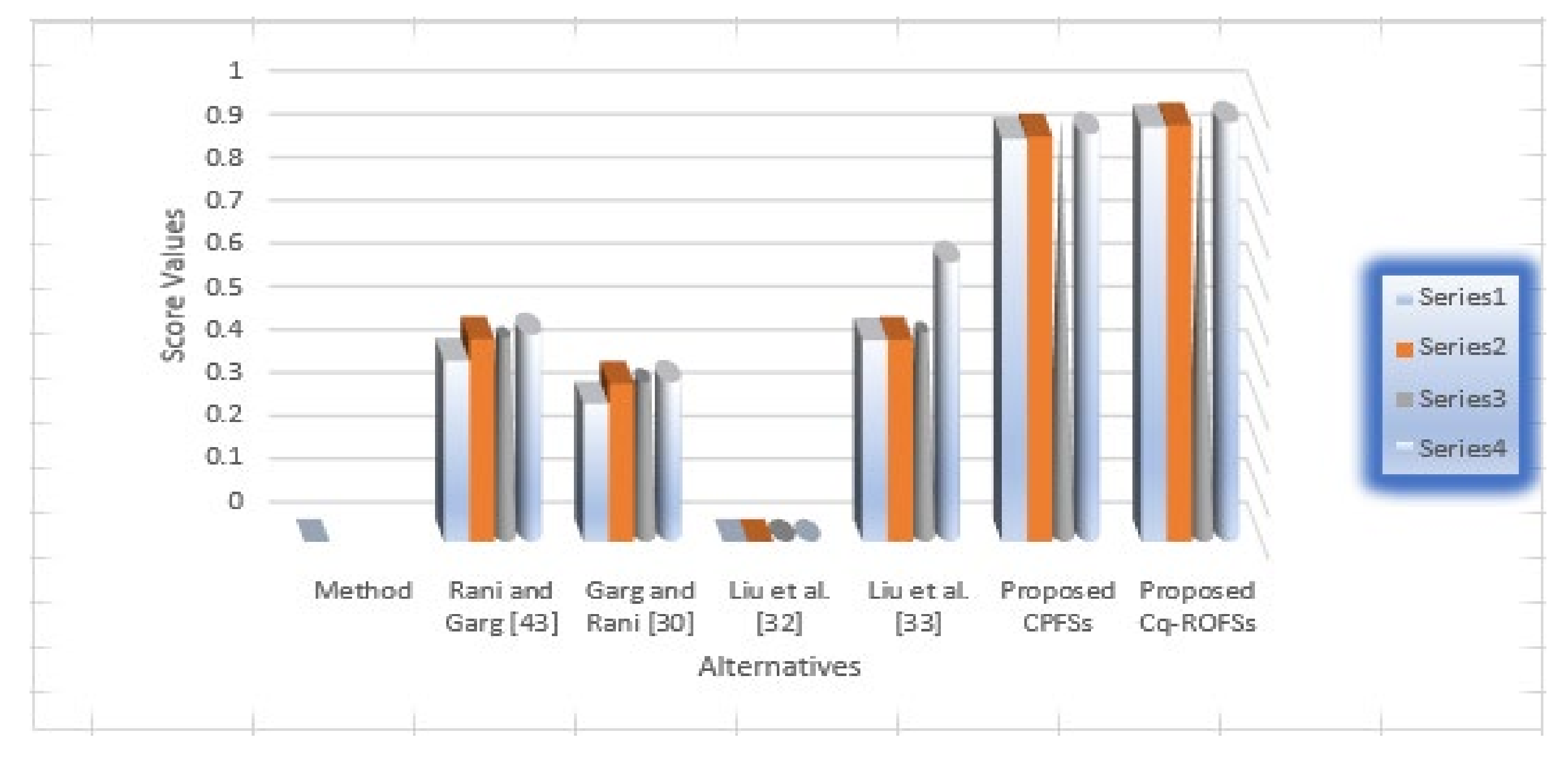
Based on the information in Table 4, we can see that there are similar positioning outcomes by utilizing the strategies proposed in [30,32,33,43] and our proposed strategy dependent on the Cq-ROFWHM operator. Although the positioning outcome dependent on the Cq-ROFWHM operator is somewhat different than the others, the best option is consistently $\mathcal{A}{L}_4$. Therefore, the strategy in this paper is viable and possible. The geometrical understanding of Table 4 is shown in Figure 1.

5. Advantages and Comparative Analysis

In this section, we direct a few correlations from a quantitative viewpoint. We used some leaving strategies to settle on a similar model and consider their last positioning outcomes. We compared our strategy and the technique proposed by Rani and Garg [43], dependent on a power collection administrator that is dependent on CIFS, and the technique proposed by Garg and Rani [30], dependent on an accumulation operator that is dependent on CIFS. The score capacities and positioning outcomes are displayed in Table 4. Be that as it may, our technique depending on the Cq-ROFWHM operators was compared, and existing strategies are discussed about in an outline model (c-f). As a matter of first importance, every one of the techniques aside from our strategy depends on CIFS. As we referenced previously, CIFS is just a unique instance of Cq-ROLS (when q = 1). Alkouri and Salleh [25] proposed the idea of CIFS. The idea of CPFS was proposed by Ullah et al. [31], which is likewise an extraordinary instance of Cq-ROLS (when q = 2). Consequently, our technique is more effective than the various other strategies.

Example 4.

In this investigation, we provide a guide to communicate the dependability and viability of the spearheaded approach. An endeavor needs to pick a provider, and there are four providers as applicants, $\mathcal{A}{L}_{\mathrm{ἷ}}=\left(\mathcal{A}{L}_1,\mathcal{A}{L}_2,\mathcal{A}{L}_3,\mathcal{A}{L}_4\right)$. We inspect every provider from four viewpoints,$G_{\mathrm{ἷ}}=\left(G_1,G_2,G_3,G_4\right)$, which are “creation cost”, “creation quality”, “provider’s administration execution”, and “hazard factor”. The weight vector of the qualities is given by$\mathrm{ὦ}={\left(0.3,0.3,0.3,0.1\right)}^T$. Then, at that point, the means of calculation to take care of the issues are as provided in

Table 5. Expressions of the complex Pythagorean fuzzy matrix.

Symbols	${\mathit{G}}_1$	${\mathit{G}}_2$	${\mathit{G}}_3$	${\mathit{G}}_4$
𝒜L1	$\left(0.5e^{\mathrm{ἷ}2\pi \left(0.44\right)},0.3e^{\mathrm{ἷ}2\pi \left(0.21\right)}\right)$	$\left(0.7e^{\mathrm{ἷ}2\pi \left(0.3\right)},0.4e^{\mathrm{ἷ}2\pi \left(0.31\right)}\right)$	$\left(0.6e^{\mathrm{ἷ}2\pi \left(0.5\right)},0.41e^{\mathrm{ἷ}2\pi \left(0.6\right)}\right)$	$\left(0.65e^{\mathrm{ἷ}2\pi \left(0.56\right)},0.4e^{\mathrm{ἷ}2\pi \left(0.5\right)}\right)$
𝒜L2	$\left(0.52e^{\mathrm{ἷ}2\pi \left(0.46\right)},0.32e^{\mathrm{ἷ}2\pi \left(0.23\right)}\right)$	$\left(0.71e^{\mathrm{ἷ}2\pi \left(0.35\right)},0.41e^{\mathrm{ἷ}2\pi \left(0.32\right)}\right)$	$\left(0.61e^{\mathrm{ἷ}2\pi \left(0.51\right)},0.42e^{\mathrm{ἷ}2\pi \left(0.52\right)}\right)$	$\left(0.66e^{\mathrm{ἷ}2\pi \left(0.57\right)},0.41e^{\mathrm{ἷ}2\pi \left(0.51\right)}\right)$
𝒜L3	$\left(0.54e^{\mathrm{ἷ}2\pi \left(0.48\right)},0.34e^{\mathrm{ἷ}2\pi \left(0.25\right)}\right)$	$\left(0.72e^{\mathrm{ἷ}2\pi \left(0.36\right)},0.42e^{\mathrm{ἷ}2\pi \left(0.33\right)}\right)$	$\left(0.62e^{\mathrm{ἷ}2\pi \left(0.52\right)},0.43e^{\mathrm{ἷ}2\pi \left(0.53\right)}\right)$	$\left(0.67e^{\mathrm{ἷ}2\pi \left(0.58\right)},0.41e^{\mathrm{ἷ}2\pi \left(0.52\right)}\right)$
𝒜L4	$\left(0.56e^{\mathrm{ἷ}2\pi \left(0.5\right)},0.36e^{\mathrm{ἷ}2\pi \left(0.27\right)}\right)$	$\left(0.73e^{\mathrm{ἷ}2\pi \left(0.37\right)},0.43e^{\mathrm{ἷ}2\pi \left(0.34\right)}\right)$	$\left(0.63e^{\mathrm{ἷ}2\pi \left(0.53\right)},0.44e^{\mathrm{ἷ}2\pi \left(0.54\right)}\right)$	$\left(0.68e^{\mathrm{ἷ}2\pi \left(0.59\right)},0.42e^{\mathrm{ἷ}2\pi \left(0.53\right)}\right)$

.

By using the investigated Cq-ROFWHM operator, the SVs of the aggregated values are presented in

Table 6. Score values of the information in Table 5.

Methods	𝒜L1	𝒜L2	𝒜L3	𝒜L4
Score values	$0.978$	$0.982$	$0.9841$	$0.984$

.

By using the information in Table 6, we obtained the ranking values, such that:

$$\mathcal{A}{L}_3\succcurlyeq \mathcal{A}{L}_4\succcurlyeq \mathcal{A}{L}_2\succcurlyeq \mathcal{A}{L}_1$$

We obtained the best optimal value in the form of $\mathcal{A}{L}_3$. By using the information in Table 5, the comparative analysis of the presented and prevailing operators is shown in

Table 7. Sensitive analysis of the explored and prevailing operators by using the information in Table 5.

Methods	Score Values	Ranking
Rani and Garg [43]	$Cannot be Calculated$	$Cannot be Calculated$
Garg and Rani [30]	$Cannot be Calculated$	$Cannot be Calculated$
Liu et al. [32]	$Cannot be Calculated$	$Cannot be Calculated$
Liu et al. [33]	$\mathrm{Ṧ}\left(\mathcal{A}{L}_1\right)=0.5724,\mathrm{Ṧ}\left(\mathcal{A}{L}_2\right)=0.6817,$ $\mathrm{Ṧ}\left(\mathcal{A}{L}_3\right)=0.7821,\mathrm{Ṧ}\left(\mathcal{A}{L}_4\right)=0.8934$	$\mathcal{A}{L}_4\succcurlyeq \mathcal{A}{L}_3\succcurlyeq \mathcal{A}{L}_2\succcurlyeq \mathcal{A}{L}_1$
Proposed methods for CPFSs	$\mathrm{Ṧ}\left(\mathcal{A}{L}_1\right)=0.954,\mathrm{Ṧ}\left(\mathcal{A}{L}_2\right)=0.958,$ $\mathrm{Ṧ}\left(\mathcal{A}{L}_3\right)=0.962,\mathrm{Ṧ}\left(\mathcal{A}{L}_4\right)=0.961$	$\mathcal{A}{L}_3\succcurlyeq \mathcal{A}{L}_4\succcurlyeq \mathcal{A}{L}_2\succcurlyeq \mathcal{A}{L}_1$
Proposed methods for Cq-ROFSs	$\mathrm{Ṧ}\left(\mathcal{A}{L}_1\right)=0.978,\mathrm{Ṧ}\left(\mathcal{A}{L}_2\right)=0.982,$ $\mathrm{Ṧ}\left(\mathcal{A}{L}_3\right)=0.984,\mathrm{Ṧ}\left(\mathcal{A}{L}_4\right)=0.984$	$\mathcal{A}{L}_3\succcurlyeq \mathcal{A}{L}_4\succcurlyeq \mathcal{A}{L}_2\succcurlyeq \mathcal{A}{L}_1$

.

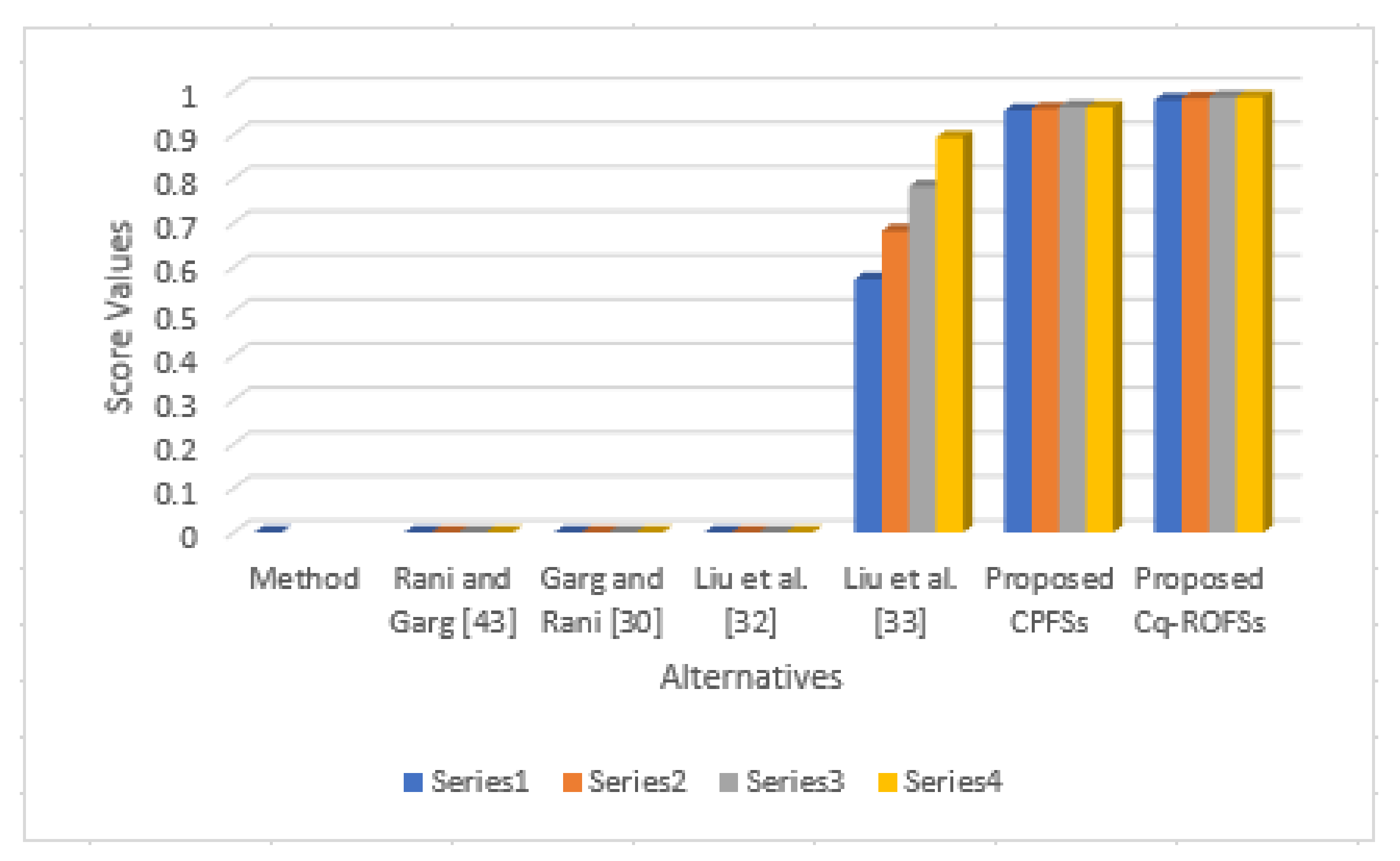
Based on the information in Table 7, we can see that there are similar positioning outcomes by utilizing the strategies proposed in [30,32,33,43] and our proposed strategy dependent on the Cq-ROFWHM operator. Although the positioning outcome dependent on the Cq-ROFWHM operator is somewhat different than the others, the best option is consistently $\mathcal{A}{L}_3$. Therefore, the strategy in this paper is viable and possible. The geometrical understanding of Table 7 is shown in Figure 2.

Example 5.

In this investigation, we provide a guide to communicate the dependability and viability of the spearheaded approach. An endeavor needs to pick a provider, and there are four providers as applicants,$\mathcal{A}{L}_{\mathrm{ἷ}}=\left(\mathcal{A}{L}_1,\mathcal{A}{L}_2,\mathcal{A}{L}_3,\mathcal{A}{L}_4\right)$. We inspect every provider from four viewpoints,$G_{\mathrm{ἷ}}=\left(G_1,G_2,G_3,G_4\right)$, which are “creation cost”, “creation quality”, “provider’s administration execution”, and “hazard factor”. The weight vector of the qualities is given by$\mathrm{ὦ}={\left(0.3,0.3,0.3,0.1\right)}^T$. Then, at that point, the means of calculation to take care of the issues are as shown in

Table 8. Expressions of the complex Pythagorean fuzzy matrix.

Symbols	${\mathit{G}}_1$	${\mathit{G}}_2$	${\mathit{G}}_3$	${\mathit{G}}_4$
𝒜L1	$\left(0.9e^{\mathrm{ἷ}2\pi \left(0.81\right)},0.3e^{\mathrm{ἷ}2\pi \left(0.21\right)}\right)$	$\left(0.81e^{\mathrm{ἷ}2\pi \left(0.9\right)},0.4e^{\mathrm{ἷ}2\pi \left(0.31\right)}\right)$	$\left(0.6e^{\mathrm{ἷ}2\pi \left(0.7\right)},0.6e^{\mathrm{ἷ}2\pi \left(0.4\right)}\right)$	$\left(0.65e^{\mathrm{ἷ}2\pi \left(0.56\right)},0.3e^{\mathrm{ἷ}2\pi \left(0.4\right)}\right)$
𝒜L2	$\left(0.92e^{\mathrm{ἷ}2\pi \left(0.82\right)},0.32e^{\mathrm{ἷ}2\pi \left(0.23\right)}\right)$	$\left(0.87e^{\mathrm{ἷ}2\pi \left(0.93\right)},0.41e^{\mathrm{ἷ}2\pi \left(0.32\right)}\right)$	$\left(0.61e^{\mathrm{ἷ}2\pi \left(0.72\right)},0.66e^{\mathrm{ἷ}2\pi \left(0.41\right)}\right)$	$\left(0.66e^{\mathrm{ἷ}2\pi \left(0.57\right)},0.29e^{\mathrm{ἷ}2\pi \left(0.1\right)}\right)$
𝒜L3	$\left(0.93e^{\mathrm{ἷ}2\pi \left(0.83\right)},0.34e^{\mathrm{ἷ}2\pi \left(0.25\right)}\right)$	$\left(0.88e^{\mathrm{ἷ}2\pi \left(0.94\right)},0.42e^{\mathrm{ἷ}2\pi \left(0.33\right)}\right)$	$\left(0.62e^{\mathrm{ἷ}2\pi \left(0.73\right)},0.59e^{\mathrm{ἷ}2\pi \left(0.42\right)}\right)$	$\left(0.67e^{\mathrm{ἷ}2\pi \left(0.58\right)},0.28e^{\mathrm{ἷ}2\pi \left(0.2\right)}\right)$
𝒜L4	$\left(0.94e^{\mathrm{ἷ}2\pi \left(0.84\right)},0.36e^{\mathrm{ἷ}2\pi \left(0.27\right)}\right)$	$\left(0.89e^{\mathrm{ἷ}2\pi \left(0.95\right)},0.43e^{\mathrm{ἷ}2\pi \left(0.34\right)}\right)$	$\left(0.63e^{\mathrm{ἷ}2\pi \left(0.74\right)},0.62e^{\mathrm{ἷ}2\pi \left(0.43\right)}\right)$	$\left(0.68e^{\mathrm{ἷ}2\pi \left(0.59\right)},0.27e^{\mathrm{ἷ}2\pi \left(0.3\right)}\right)$

.

By using the investigated Cq-ROFWHM operator, the SVs of the aggregated values are shown in

Table 9. Score values of the information in Table 8.

Methods	𝒜L1	𝒜L2	𝒜L3	𝒜L4
Score values	$0.999879$	$0.999936$	$0.999955$	$0.99997$

for $\zeta =4$.

By using the information in Table 9, we obtained the ranking values, such that:

$$\mathcal{A}{L}_4\succcurlyeq \mathcal{A}{L}_3\succcurlyeq \mathcal{A}{L}_2\succcurlyeq \mathcal{A}{L}_1$$

We obtained the best optimal value in the form of $\mathcal{A}{L}_4$. By using the information in Table 8, the comparative analysis of the presented and prevailing operators is shown in

Table 10. Sensitive analysis of the explored and prevailing operators by using the information in Table 8.

Methods	Score Values	Ranking
Rani and Garg [43]	$Cannot be Calculated$	$Cannot be Calculated$
Garg and Rani [30]	$Cannot be Calculated$	$Cannot be Calculated$
Liu et al. [32]	$Cannot be Calculated$	$Cannot be Calculated$
Liu et al. [33]	$\mathrm{Ṧ}\left(\mathcal{A}{L}_1\right)=0.6835,\mathrm{Ṧ}\left(\mathcal{A}{L}_2\right)=0.7928,$ $\mathrm{Ṧ}\left(\mathcal{A}{L}_3\right)=0.8932,\mathrm{Ṧ}\left(\mathcal{A}{L}_4\right)=0.9945$	$\mathcal{A}{L}_4\succcurlyeq \mathcal{A}{L}_3\succcurlyeq \mathcal{A}{L}_2\succcurlyeq \mathcal{A}{L}_1$
Proposed methods for CPFSs	$Cannot be Calculated$	$Cannot be Calculated$
Proposed methods for Cq-ROFSs	$\mathrm{Ṧ}\left(\mathcal{A}{L}_1\right)=0.999879,\mathrm{Ṧ}\left(\mathcal{A}{L}_2\right)=0.999936,$ $\mathrm{Ṧ}\left(\mathcal{A}{L}_3\right)=999955,\mathrm{Ṧ}\left(\mathcal{A}{L}_4\right)=099997$	$\mathcal{A}{L}_4\succcurlyeq \mathcal{A}{L}_3\succcurlyeq \mathcal{A}{L}_2\succcurlyeq \mathcal{A}{L}_1$

.

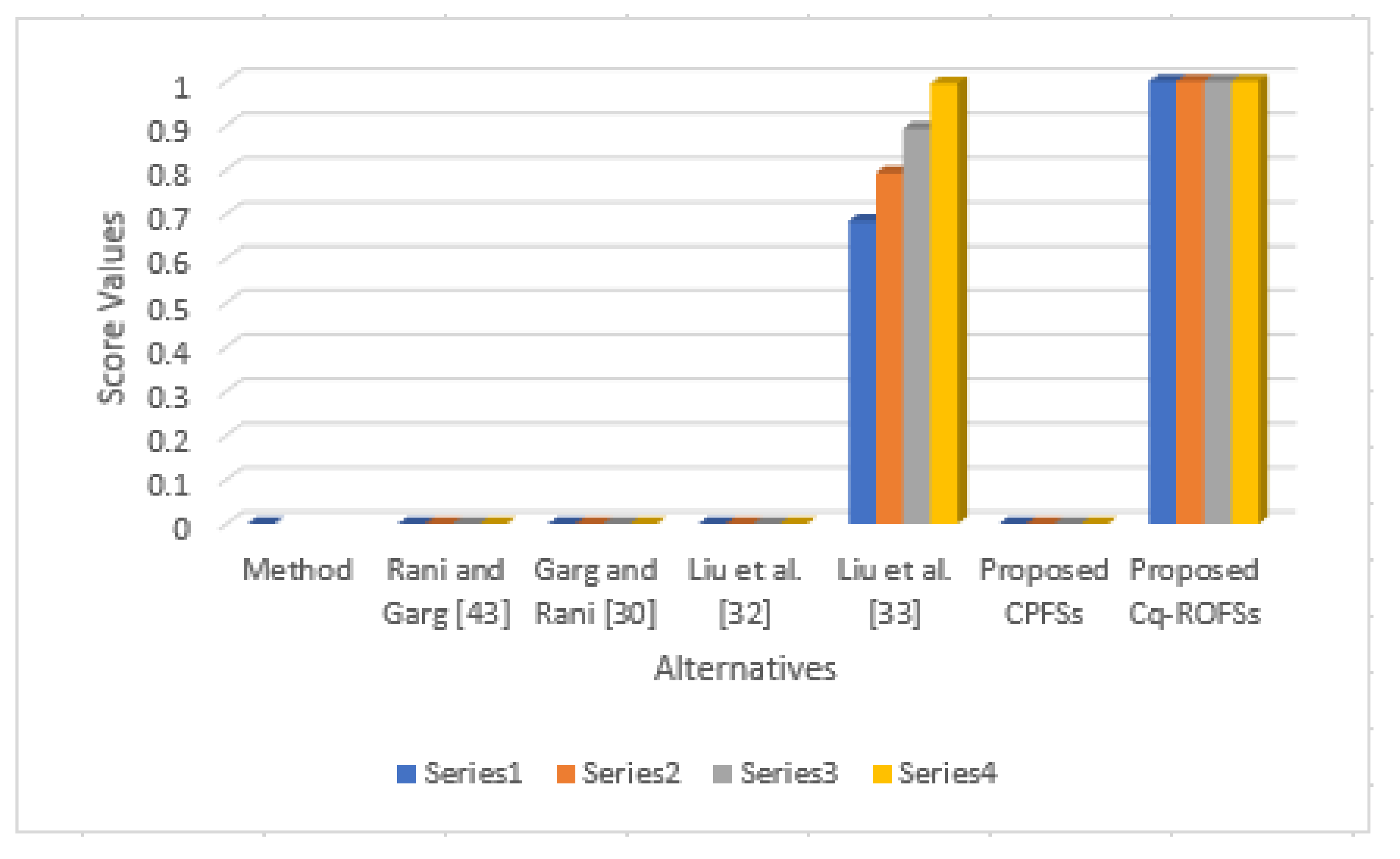
Based on the information in Table 10, we can see that there are similar positioning outcomes by utilizing the strategies proposed in [30,32,33,43] and our proposed strategy dependent on the Cq-ROFWHM operator. Although the positioning outcome dependent on the Cq-ROFWHM operator is somewhat different than the others, the best option is consistently $\mathcal{A}{L}_4$. Therefore, the strategy in this paper is viable and possible. The geometrical understanding of Table 10 is shown in Figure 3.

Therefore, the initiated operators under the Cq-ROFNs are very powerful and more dominant as compared to prevailing ideas [30,43].

6. Conclusions

Several researchers have changed the hypothesis of FSs, however the guidelines of complex QROFS have gained increasing attention from various researchers. In this paper, we have provided an examination of CQROFS and their aggregation operators dependent on the HM and weighted HM operators and their application in MADM. To improve the Cq-ROFNs, the Cq-ROFHM administrator and Cq-ROFWHM administrator have been developed. Additionally, we have applied the Cq-ROFWHM administrator to take care of the MADM issues. Finally, a useful test for undertaking execution framework determination was provided to confirm the proposed approach and to show its practicality and viability. Using the proposed model, we have generally shown that the boundaries of the conglomeration operation operators affect the positions of choices. The Cq-ROFHM and Cq-ROFWHM administrators were distinguished from other existing administrators not only because of the way that the administrators oblige the Cq-ROFNs, but also because of the consideration of the related issues among the contentions, which permits our administrators to have all the wider commonsense application possibilities.

In future research, the use of the proposed improved administrators of Cq-ROFSs should be investigated in the different fuzzy climates [44,45]. Additionally, we will extend the approach to solve different problems, such as solid waste management [46], medical diagnosis [47], bipartite graph theory [48], etc.