Modelling the Phosphorylation of Glucose by Human hexokinase I

Abstract

In this paper, we develop a comprehensive mathematical model to describe the phosphorylation of glucose by the enzyme hexokinase I. Glucose phosphorylation is the first step of the glycolytic pathway, and as such, it is carefully regulated in cells. Hexokinase I phosphorylates glucose to produce glucose-6-phosphate, and the cell regulates the phosphorylation rate by inhibiting the action of this enzyme. The cell uses three inhibitory processes to regulate the enzyme: an allosteric product inhibitory process, a competitive product inhibitory process, and a competitive inhibitory process. Surprisingly, the cellular regulation of hexokinase I is not yet fully resolved, and so, in this study, we developed a detailed mathematical model to help unpack the behaviour. Numerical simulations of the model produced results that were consistent with the experimentally determined behaviour of hexokinase I. In addition, the simulations provided biological insights into the abstruse enzymatic behaviour, such as the dependence of the phosphorylation rate on the concentration of inorganic phosphate or the concentration of the product glucose-6-phosphate. A global sensitivity analysis of the model was implemented to help identify the key mechanisms of hexokinase I regulation. The sensitivity analysis also enabled the development of a simpler model that produced an output that was very close to that of the full model. Finally, the potential utility of the model in assisting experimental studies is briefly indicated.

1. Introduction

Glucose is a major source of energy for most living organisms. Glucose glycolysis is a key pathway for the production of energy in a cell [1], and glycolytic intermediates form precursors for the biosynthesis of other key cellular constituents, such as glycogen, nucleotide sugars, and hyaluronan. The first step of glycolysis is the transformation of glucose into glucose-6-phosphate. This is achieved via a phosphorylation that is catalysed by an enzyme called hexokinase. There are four isozymes of hexokinase found in mammalian tissue [2,3], and these are usually referred to as hexokinase I, II, III, and IV (glucokinase). The molecular weights for hexokinase I, II, and III are all approximately 100 kDa. However, hexokinase IV is a smaller molecule, with a molecular weight of approximately 50 kDa [4].

Previous studies have identified some of the functions and expression levels for the various hexokinase isoforms. Hexokinase I is present in all tissues, where it regulates the rate-limiting step of glycolysis; the mechanism of this regulation forms the topic of the current study. It is the predominant form present in brain cells and red blood cells [5,6]. Hexokinase II is known to be highly expressed in skeletal muscle and adipose tissue [7,8]. Hexokinase III is typically present at low levels in most tissues, with the highest levels being found in the lung, the kidney, and the liver [9,10,11]. Finally, glucokinase is primarily expressed in hepatocytes and pancreatic $\beta$ cells [12,13].

Abnormal levels of hexokinase in cells are known to be linked to a number of diseases. Hexokinase I deficiency is known to be associated with hemolytic anaemia; see [14,15] and the references therein. Hemolytic anaemia is a form of anaemia caused by an abnormally high level of red blood cell destruction in the body. On the other hand, overexpression of hexokinase I is associated with increased levels of basal insulin release [16]. For a therapeutic effect, the results of [17] suggest that overexpression of hexokinase II in endothelial cells can help reverse microvascular disease.

Hexokinase I and II can bind to the outer membrane of mitochondria, a process that has been associated with the prevention of cell death [18,19]. Hexokinase III does not bind to mitochondria and exists predominantly in the cytoplasmic fraction, although there is evidence for hexokinase III perinuclear binding [20]. Hexokinase III overexpression has been associated with a reduction in cell death [21]. As hexokinase III, hexokinase IV (glucokinase) cannot bind to mitochondria and is localised in the cytoplasm, where it plays a key role in the regulation of glucose homoeostasis [22].

The product of glucose phosphorylation, glucose-6-phosphate ($G6P$), inhibits the activity of hexokinase I, II, and III (but not glucokinase) at physiological levels. Inorganic phosphate ($P_i$), however, antagonises the inhibition of hexokinase I by glucose-6-phosphate at low concentrations (few millimolar) and becomes an inhibitor of hexokinase I at high concentrations. In addition, inorganic phosphate inhibits hexokinases II and III at all concentrations [11,21,23]. Only the C-terminal half of hexokinase I contains the catalytic sites, whereas the N-terminal half does not [23,24], but is involved in the $P_i$-antagonism of the product inhibition [24,25]. In contrast, both the C- and N-terminal halves of hexokinase II are catalytically active and sensitive to $G6P$ levels [26,27]. Furthermore, both hexokinase I and II have binding sites for $ATP$, glucose, $G6P$, and $P_i$ in both N- and C-terminal halves [4,24,28]. Similar to hexokinase I, only the C-terminal half of hexokinase III is catalytically active [29,30]. A detailed description of the kinetic mechanism for hexokinase I is given in the next section.

In this study, we for the first time synthesize the current state of knowledge of the cellular regulation of hexokinase I into a comprehensive mathematical model. The model incorporates numerous bound states for the enzyme, together with their associated activation status. Numerical simulations of the model produced results that were consistent with the experimentally determined behaviour of hexokinase I. Simulations of the model provided biological insights into the abstruse enzymatic behaviour, such as the dependence of the phosphorylation rate on the concentration of inorganic phosphate or the concentration of the product glucose-6-phosphate. A global sensitivity analysis of the model was implemented to help identify the key mechanisms of hexokinase I regulation. The sensitivity analysis enabled the development of a simpler model that produced an output that was very close to that of the full model. Finally, the potential utility of the model in assisting experimental studies is indicated.

2. Materials and Methods

2.1. Mathematical Model

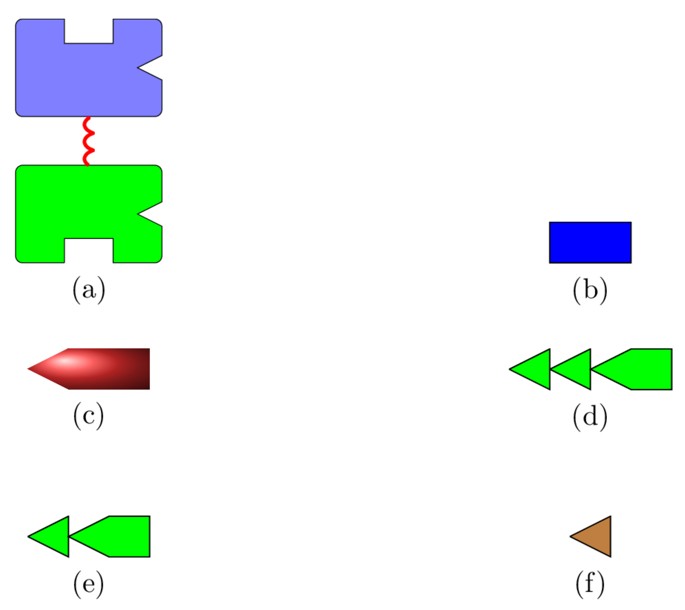
Many cellular factors can influence the phosphorylation of glucose by hexokinase I. In the current paper, we constructed a mathematical model that describes the cellular regulation of glucose phosphorylation. One of the principal aims of the modelling was to gain insight into the roles of $G6P$ and $P_i$ in regulating the phosphorylation process. The model consisted of a system of ordinary differential equations that tracks the evolution in time of the concentrations of various relevant species, including hexokinase enzyme, glucose, $G6P$, $ATP$, $ADP$, and $P_i$. We give schematic representations for each of these species in Figure 1.

Figure 1a represents a single hexokinase I molecule, with blue being used for the N-terminal domain and green for the C-terminal domain. Each hexokinase I molecule possesses binding sites for glucose, $ATP$, $G6P$, and inorganic phosphate in the both the C- and N-domains, even though the C-domain is only catalytically active [4,23,24]. In Figure 1a, the binding sites for glucose on the C- and N-domains are depicted by the ⊔ shape and the binding sites for $ATP$, glucose-6-phosphate, and inorganic phosphate are represented by a ∨ cleft.

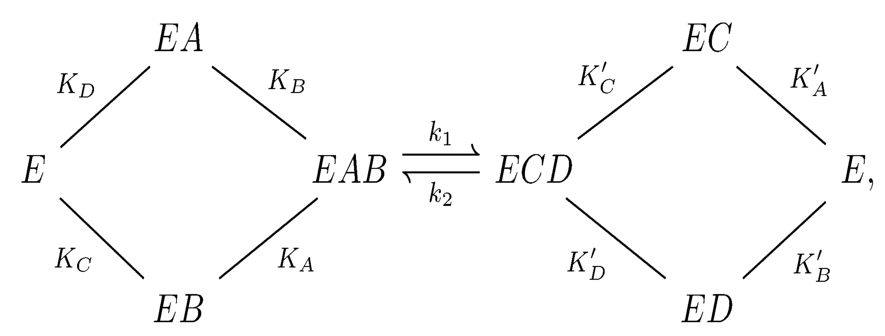
In 1969, Ning et al. [31] proposed a random Bi Bi kinetic mechanism for hexokinase I. This mechanism is represented by the chemical equations shown in Figure 2. There is considerable experimental evidence in support of the Bi Bi mechanism for hexokinase I; see [4,32,33,34,35]. In the context of the current study, it forms a part of a larger kinetic mechanism we developed for hexokinase I.

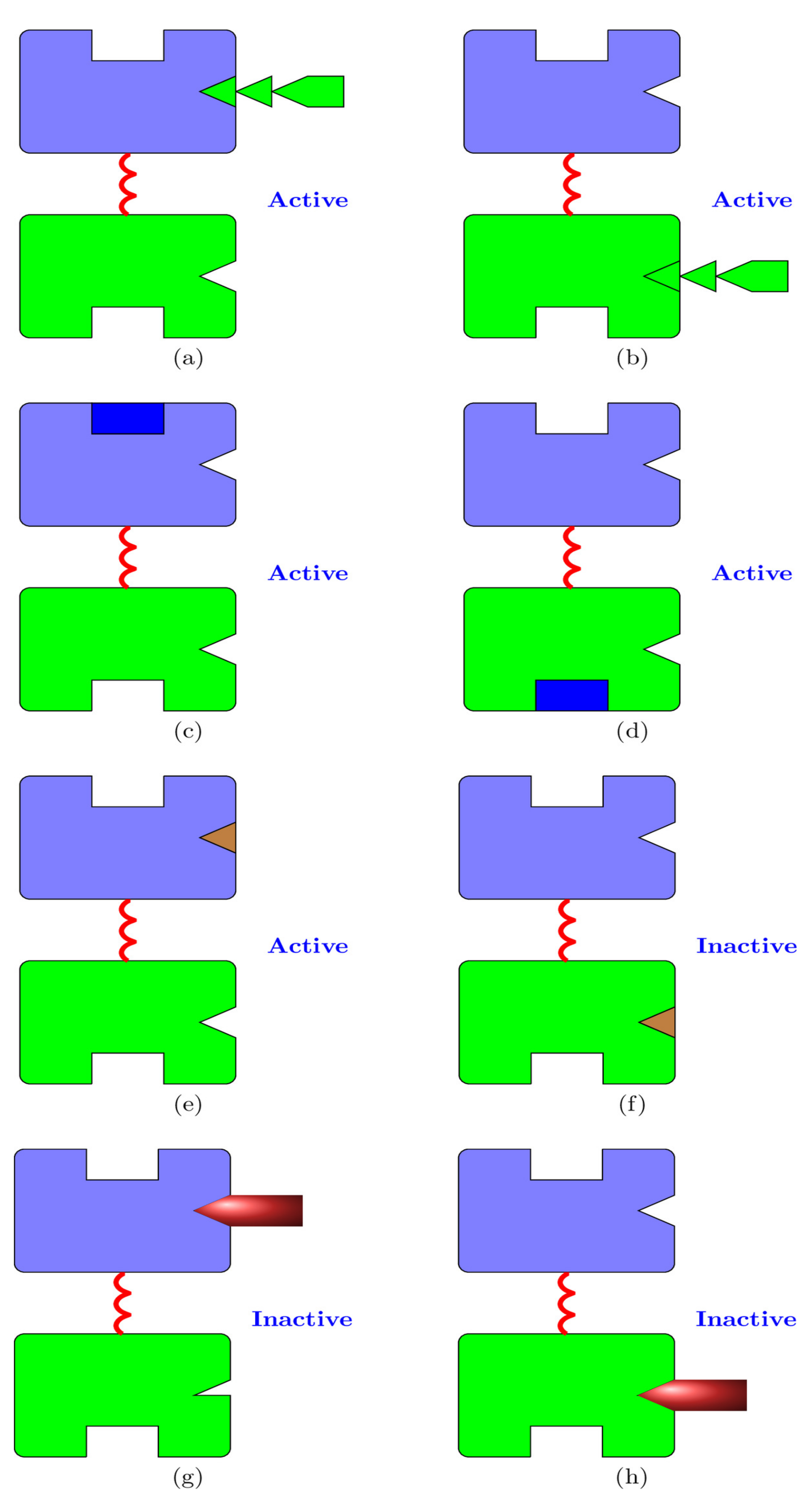
The mathematical model we developed for the phosphorylation of glucose is necessarily large and complex since it describes multiple binding sites, numerous species, almost 150 chemical reactions, and various inhibitory mechanisms. The phosphorylation mechanism of glucose by hexokinase I was already briefly introduced in the Introduction Section, and schematic representations of the relevant species arising are given in Figure 1. Recall that each hexokinase I molecule has two subunits, an N- and a C-terminal domain. Each subunit has its own binding site for glucose and another binding site for $ATP$, $P_i$, and $G6P$ [4]. In Figure 3, we depict the eight possible configurations of the molecule where only one of the binding sites is occupied.

2.1.1. The Kinetic Mechanism

The kinetic mechanism for the phosphorylation of glucose by hexokinase I may be summarized as follows:

• Binding sites: Both the N- and C-domains have two binding sites: one for glucose and another for $ATP$, $P_i$, and $G6P$ [4,25,36,37,38,39,40,41,42]; see Figure 3;
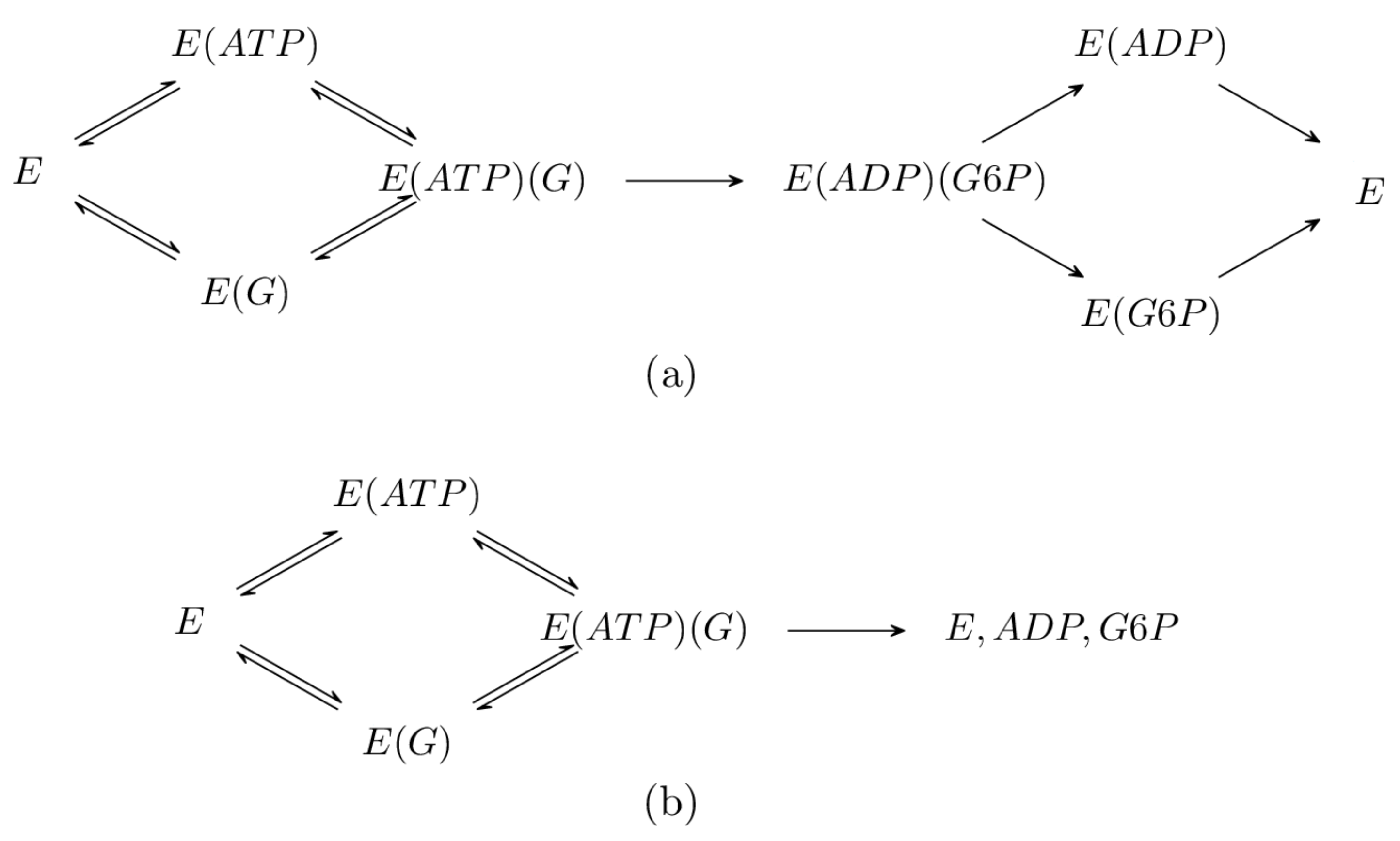
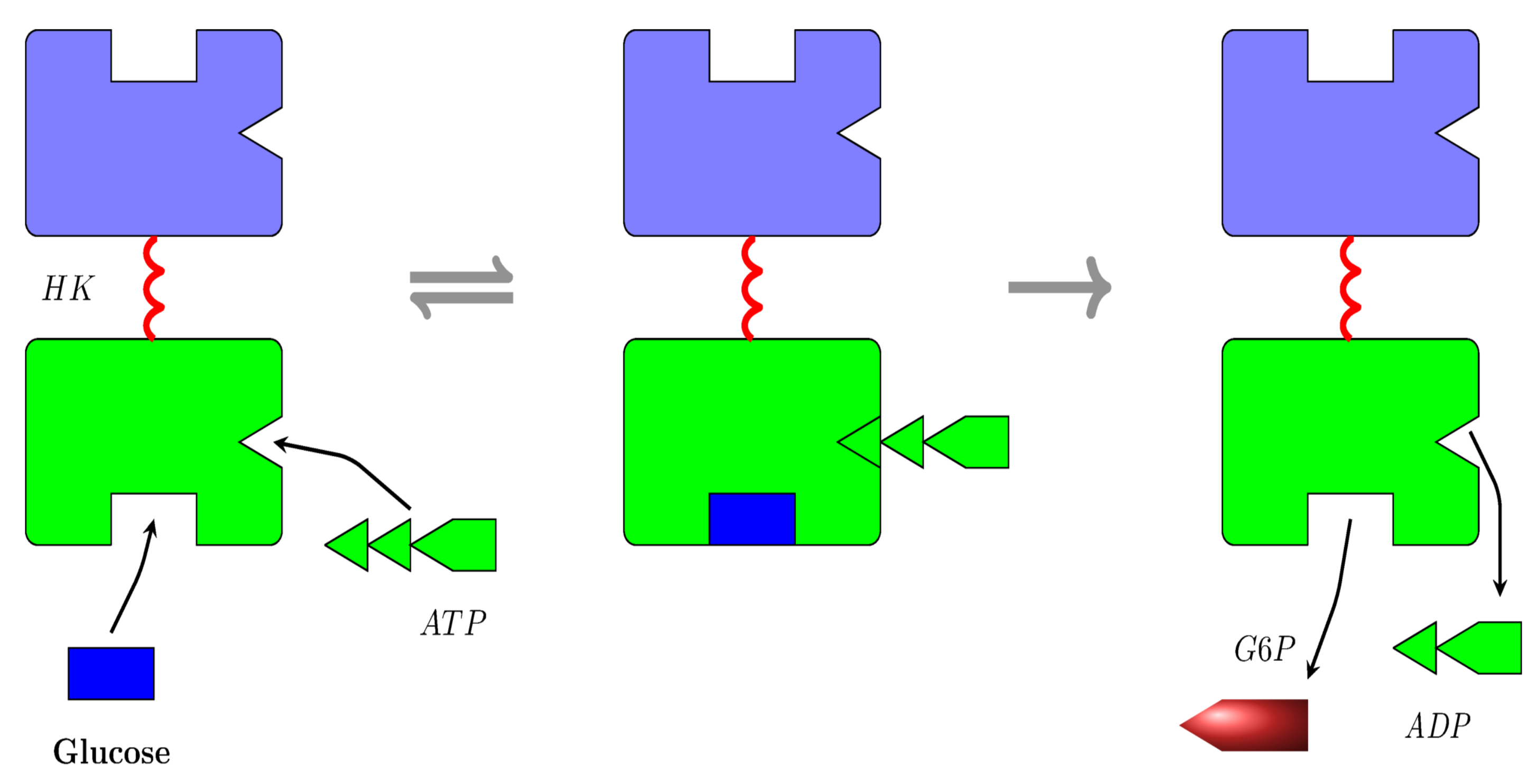
• Product production: The product here is $G6P$, and it is produced by the phosphorylation of glucose by hexokinase I. The phosphorylation is achieved via a Bi Bi mechanism [31], as represented in Figure 4a. However, in the current study, we considered the simplified process represented in Figure 4b. This is partially justified by noting that the simplified mechanism produces the same ultimate products as the Bi Bi mechanism, that is E, $ADP$, and $G6P$. This is because all of the reactions in the right branch of the Bi Bi mechanism are essentially irreversible; see Section 16.2 of [43]. Here, for a $G6P$ molecule to be produced, an $ATP$ molecule must be bound to its C-domain site and a glucose molecule must be bound to its C-domain site; see Figure 5;
• Product production is regulated: The phosphorylation of glucose is inhibited via the following three mechanisms:

  (a)

  Competitive inhibition: $P_i$ competes with $ATP$ for the C-domain binding site; see Figure 3f.

  (b)

  Allosteric product inhibition [44]. Binding of a molecule of $G6P$ to the N-binding site makes a conformational change to the C-domain binding site for $ATP$. This conformational change disables the binding of $ATP$ to the C-domain, resulting in the deactivation of the enzyme [37,38]; see Figure 3g. This inhibition is mitigated by the presence of $P_i$ and $ATP$, which compete with $G6P$ for the N-domain binding site;

  (c)

  Competitive product inhibition: The product $G6P$ competes with $ATP$ for its C-domain binding site, inhibiting product production; see Figure 3h;

• Other details: The following information concerning glucose phosphorylation is also available in the literature:

  (a)

  Only one molecule of $G6P$ can bind to an enzyme molecule at a time [37,38];

  (b)

  The binding of $P_i$ to the N-domain binding site weakens the binding of $G6P$ to the C-domain binding site (that is, it increases the dissociation constant) [39,41];

  (c)

  The $ATP$ binding sites of free or complexed enzyme are open, except for the case where a $G6P$ molecule is bound at the N-binding site;

  (d)

  The high-affinity binding site for $G6P$ is in the C-domain, while the high affinity binding site for $P_i$ is in N-domain [39].

2.1.2. Modelling Assumptions

(a)

It was assumed throughout that the cellular mixture of hexokinase I, glucose, $ATP$, and $P_i$ is well-stirred. This implies that diffusive effects in the phosphorylation process can be neglected and that the concentrations of the various species in the mixture can be described by functions of time only. This further implies that the evolution of the system can be modelled by a coupled system of nonlinear ordinary differential equations and that a partial differential equation model is not required;

(b)

We assumed mass action kinetics throughout [45]; this implies that the rate of a reaction is taken to be proportional to the product of the concentrations of the reactants. We emphasise here that more complex formulae, such as the Michaelis–Menten formula for the rate of product production in an enzyme-catalysed reaction, are derivable from more fundamental mass action considerations under simplifying assumptions [46];

(c)

We focused our attention solely on the phosphorylation of glucose and made no attempt to model in detail the evolution of the intracellular glucose concentration. Rather, we assumed instead a constant initial concentration of glucose and used the model to track its subsequent depletion as it is converted to $G6P$ via phosphorylation;

(d)

The mechanism of the phosphorylation of glucose was assumed to be the simplified Bi Bi process represented in Figure 4b;

(e)

The binding of one substrate does not affect the affinity of the binding sites for other substrates, except that the binding of $P_i$ at the N-domain reduces the affinity of the C-binding site for $G6P$;

(f)

The model allows only one molecule of $G6P$ to bind to an enzyme molecule at a time.

2.1.3. Model Notation

We introduce the following model notation. We write:

$$\begin{array}{cccc}\hfill E& :\mathrm{a}\mathit{hexokinase}I\mathrm{molecule};\hfill & \hfill G& :\mathrm{a}\mathrm{glucose}\mathrm{molecule};\hfill \\ \hfill T& :\mathrm{an}ATP\mathrm{molecule};\hfill & \hfill G6& :\mathrm{a}G6P\mathrm{molecule};\hfill \\ \hfill P& :\mathrm{a}{P}_i\mathrm{molecule};\hfill & \hfill D& :\mathrm{an}ADP\mathrm{molecule}.\hfill \end{array}$$

We also added subscripts and superscripts to E, where a subscript denotes a molecule binding to the C-domain of the enzyme and a superscript denotes a molecule binding to its N-domain. Hence, for example, we have:

$$\begin{array}{ccc}\hfill {}_{G}E& -& \mathrm{A}\mathit{hexokinase}I\mathrm{molecule}\mathrm{with}\mathrm{a}\mathrm{glucose}\mathrm{molecule}\mathrm{bound}\hfill \\ & & \mathrm{to}\mathrm{its}C-\mathrm{domain};\hfill \\ \hfill E^T& -& \mathrm{A}\mathit{hexokinase}I\mathrm{molecule}\mathrm{with}\mathrm{an}ATP\mathrm{molecule}\mathrm{bound}\hfill \\ & & \mathrm{to}\mathrm{its}N-\mathrm{domain};\hfill \\ \hfill {}^G{E}_{G6}& -& \mathrm{A}\mathit{hexokinase}I\mathrm{molecule}\mathrm{with}\mathrm{a} G6P\mathrm{molecule}\mathrm{bound}\hfill \\ & & C-\mathrm{domain}\mathrm{and}\mathrm{a}\mathrm{glucose}\mathrm{molecule}\mathrm{bound}\mathrm{to}\mathrm{its}N-\mathrm{domain};\hfill \\ \hfill {}_G{E}_P^{G6}& -& \mathrm{A}\mathit{hexokinase}I\mathrm{molecule}\mathrm{with}\mathrm{a} P_i\mathrm{molecule}\mathrm{and}\mathrm{a}\mathrm{glucose}\mathrm{molecule}\hfill \\ & & \mathrm{bound}\mathrm{to}\mathrm{its}C-\mathrm{domain}\mathrm{and}\mathrm{a} G6P\mathrm{molecule}\mathrm{bound}\mathrm{to}\mathrm{its}N-\mathrm{domain}.\hfill \end{array}$$

There are 59 such enzyme complexes in total, and adding the 6 uncomplexed species listed at the beginning of this subsection, we see that the model tracks 65 species in all; see Figure 6 and Figure 7 and the Supplementary Material. The concentration of a species X at time t is denoted by $\left[X\right]\left(t\right)$.

We introduce the following notation for the model rate constants.

$$\begin{array}{cc}\hfill k_0:& \mathrm{the}\mathrm{catalytic}\mathrm{constant}(\mathrm{turnover}\mathrm{rate})\mathrm{for}\mathit{hexokinase}I;\hfill \\ \hfill k^G,k^T,k^{G6},k^P:& \mathrm{the}\mathrm{forward}\mathrm{rate}\mathrm{constants}\mathrm{for}\mathrm{the}\mathrm{binding}\mathrm{of}\mathrm{glucose},ATP,G6P,\hfill \\ \hfill & \mathrm{and}{P}_i,\mathrm{respectively},\mathrm{to}\mathrm{their}N-\mathrm{binding}\mathrm{sites};\hfill \\ \hfill k^{-G},k^{-T},k^{-G6},k^{-P}:& \mathrm{the}\mathrm{reverse}\mathrm{rate}\mathrm{constants}\mathrm{for}\mathrm{the}\mathrm{dissociation}\mathrm{of}\mathrm{glucose},ATP,\hfill \\ \hfill & G6P,\mathrm{and}{P}_i,\mathrm{respectively},\mathrm{from}\mathrm{their}N-\mathrm{binding}\mathrm{sites};\hfill \\ \hfill k_G,k_T,k_{G6},k_P:& \mathrm{the}\mathrm{forward}\mathrm{rate}\mathrm{constants}\mathrm{for}\mathrm{the}\mathrm{binding}\mathrm{of}\mathrm{glucose},ATP,G6P,\hfill \\ \hfill & \mathrm{and}{P}_i,\mathrm{respectively},\mathrm{to}\mathrm{their}C-\mathrm{binding}\mathrm{sites};\hfill \\ \hfill k_{-G},k_{-T},k_{-G6},k_{-P}:& \mathrm{the}\mathrm{reverse}\mathrm{rate}\mathrm{constants}\mathrm{for}\mathrm{the}\mathrm{dissociation}\mathrm{of}\mathrm{glucose},ATP,\hfill \\ \hfill & G6P,\mathrm{and}{P}_i,\mathrm{respectively},\mathrm{from}\mathrm{their}C-\mathrm{binding}\mathrm{sites};\hfill \\ \hfill k_{G6}^P,k_{-G6}^P:& \mathrm{the}\mathrm{forward}\mathrm{and}\mathrm{reverse}\mathrm{rate}\mathrm{constants}\mathrm{for}\mathrm{the}\mathrm{binding}/\mathrm{unbinding}\hfill \\ \hfill & \mathrm{of}G6P\mathrm{to}/\mathrm{from}\mathrm{its}C-\mathrm{binding}\mathrm{site},\mathrm{when}\mathrm{the}\mathrm{enzyme}\mathrm{has}\mathrm{a}{P}_i\hfill \\ \hfill & \mathrm{molecule}\mathrm{bound}\mathrm{to}\mathrm{its}N-\mathrm{binding}\mathrm{site}.\hfill \end{array}$$

2.1.4. The Chemical Reactions

The system has numerous chemical reactions because of the large number of possible bound states for the enzyme, and a small selection of these is given by:

$$\begin{array}{cccc}E+G\underset{k^{-G}}{\overset{k^G}{\rightleftharpoons }}{}^{G}E,& E+G\underset{k_{-G}}{\overset{k_G}{\rightleftharpoons }}{}_{G}E,& E+T\underset{k^{-T}}{\overset{k^T}{\rightleftharpoons }}{E}^T,& E+T\underset{k_{-T}}{\overset{k_T}{\rightleftharpoons }}{E}_T,\\ E+G6\underset{k^{-\mathrm{G6}}}{\overset{k^{\mathrm{G6}}}{\rightleftharpoons }}{E}^{G6},& E+G6\underset{k_{-\mathrm{G6}}}{\overset{k_{\mathrm{G6}}}{\rightleftharpoons }}{E}_{G6},& \dots \dots \dots \dots \dots & \end{array}$$

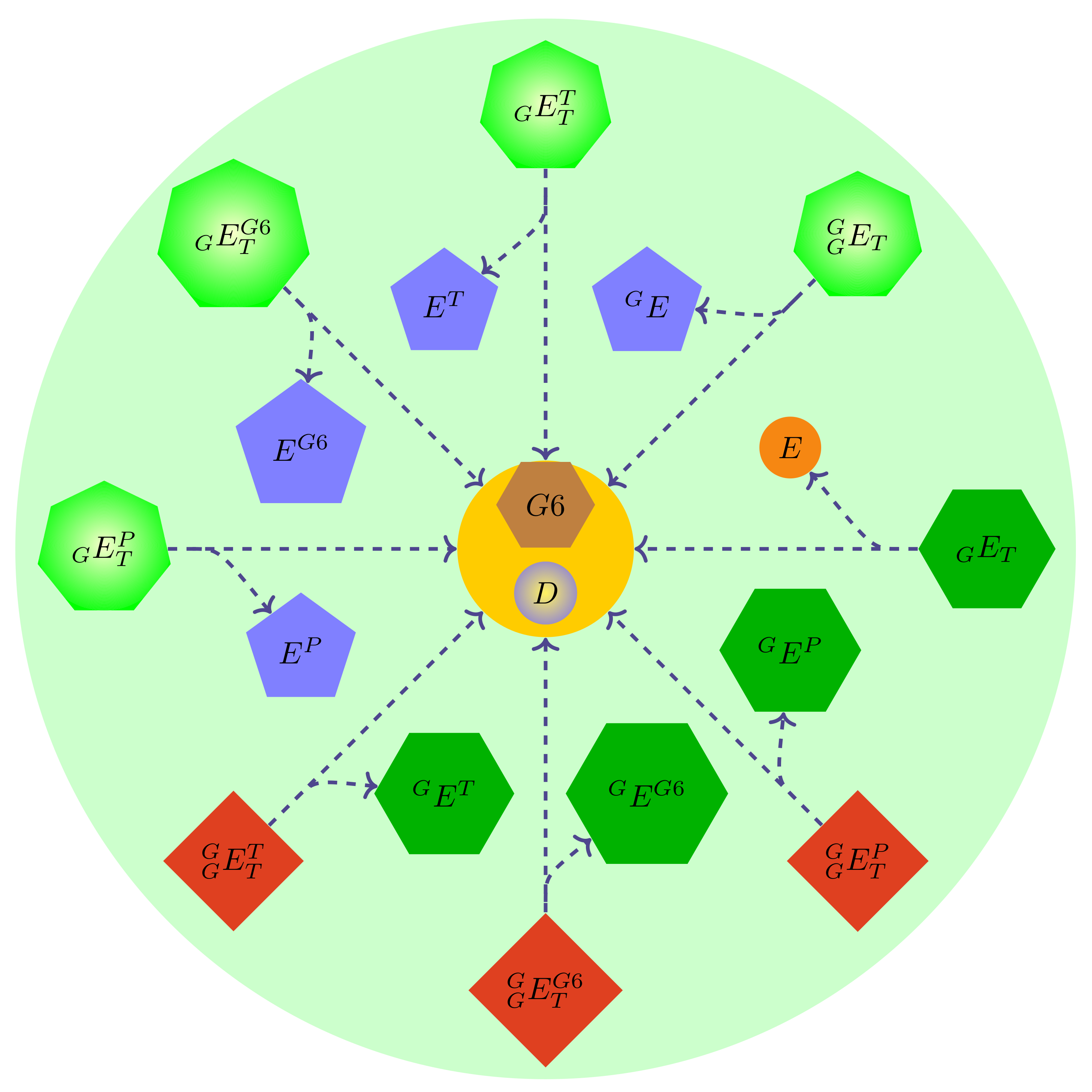
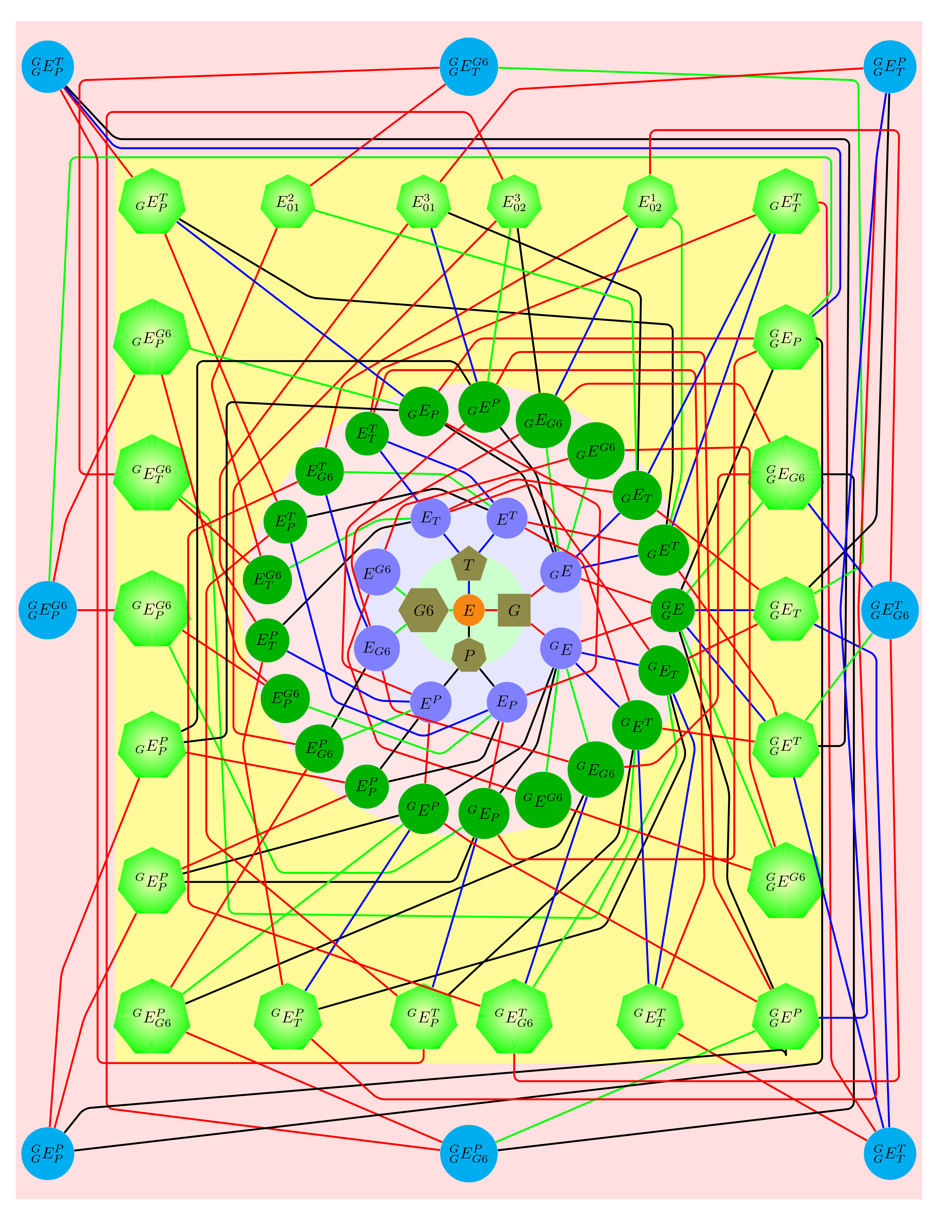
There are 147 reactions in all, and these are listed in detail in the Supplementary Material. In Figure 7, we schematically represent all of the chemical reactions producing an enzyme complex. Figure 6 shows the reactions that lead to the production of the product $G6P$.

2.1.5. Construction of the Governing Ordinary Differential Equations

The complete set of governing equations for the model can be found in the Supplementary Material, but it is not necessary to discuss all of these equations here. However, we do briefly discuss two of them to illustrate how the governing equations are constructed. The equations were developed based on the chemical reactions referred to in the previous subsection and the law of mass action. We begin by considering the equation for the product $G6P$, which is given by:

$$\begin{array}{cc}\hfill {\displaystyle \frac{d\left[G6\right]}{dt}}& =\stackrel{a}{\overbrace{k_0\left({[}_G{E}_T]+{[}_G^G{E}_T]+{[}_G{E}_T^T]+{[}_G{E}_T^{G6}]+{[}_G{E}_T^P]+{[}_G^G{E}_T^T]{+[}_G^G{E}_T^{G6}+{[}_G^G{E}_T^P]\right)}}\hfill \\ \hfill & +\stackrel{b}{\overbrace{k^{-G6}\left(\left[E^{G6}\right]+{[}^G{E}^{G6}]+{[}_G{E}^{G6}]+\left[E_T^{G6}\right]+\left[E_P^{G6}\right]+{[}_G^G{E}^{G6}]+{[}^G{E}_T^{G6}]+{[}^G{E}_P^{G6}]\right.}}\hfill \\ \hfill & \left.+{[}_G{E}_T^{G6}]+{[}_G{E}_P^{G6}]+{[}_G^G{E}_T^{G6}]+{[}_G^G{E}_P^{G6}]\right)\hfill \\ \hfill & +\stackrel{c}{\overbrace{k_{-G6}\left(\left[E_{G6}\right]+{[}_G{E}_{G6}]+{[}^G{E}_{G6}]+\left[E_{G6}^T\right]+{[}_G^G{E}_{G6}]+{[}_G{E}_{G6}^T]+{[}^G{E}_{G6}^T]+{[}_G^G{E}_{G6}^T]\right)}}\hfill \\ \hfill & +\stackrel{d}{\overbrace{k_{-G6}^P\left(\left[E_{G6}^P\right]+{[}^G{E}_{G6}^P]+{[}_G{E}_{G6}^P]+{[}_G^G{E}_{G6}^P]\right)}}\hfill \\ \hfill & -\stackrel{e}{\overbrace{\left[G6\right]\left((k^{G6}+k_{G6})(\left[E\right]+{[}^{G}E]+{[}_{G}E]+{[}_G^{G}E])+k^{G6}(\left[E_T\right]+{[}^G{E}_T]+\left[E_P\right]\right.}}\hfill \\ \hfill & +{[}^G{E}_P]+{[}_G{E}_T]+{[}_G{E}_P]+{[}_G^G{E}_T]+{[}_G^G{E}_P])\hfill \\ \hfill & +k_{G6}^P(\left[E^P\right]+{[}_G{E}^P]+{[}^G{E}^P]+{[}_G^G{E}^P])\hfill \\ \hfill & \left.+k_{G6}(\left[E^T\right]+{[}_G{E}^T]+{[}^G{E}^T]+{[}_G^G{E}^T])\right),\hfill \end{array}$$

(1)

where:

a 

These terms account for the increase in the concentration of $G6P$ due to the creation of product by enzymatic reactions involving the complexes ${}_G{E}_T$, ${}_G^G{E}_T$, ${}_G{E}_T^i$, and ${}_G^G{E}_T^i$, where $i=T,G6,P$; see Figure 6;

b 

The increase in the concentration of $G6P$ due to $G6P$ unbinding from the enzyme complexes $E^{G6}$, ${}^G{E}^{G6}$, ${}_G{E}^{G6}$, ${}_G^G{E}^{G6}$, $E_i^{G6}$, ${}^G{E}_i^{G6}$, ${}_G^G{E}_i^{G6}$, and ${}_G^G{E}_i^{G6}$, where $i=T,P$; see Figure 7;

c 

The increase in the concentration of $G6P$ due to $G6P$ unbinding from the enzyme complexes $E_{G6}$, ${}_G{E}_{G6}$, ${}^G{E}_{G6}$, $E_{G6}^T$,${}_G^G{E}_{G6}$, ${}_G{E}_{G6}^T$, ${}^G{E}_{G6}^T$, and ${}_G^G{E}_{G6}^T$ see Figure 7;

d 

The increase in the concentration of $G6P$ due to $G6P$ unbinding from the complexes $E_{G6}^P$, ${}^G{E}_{G6}^P$, ${}_G{E}_{G6}^P$, and ${}_G^G{E}_{G6}^P$; see Figure 7;

e 

The reduction in concentration of $G6P$ due to $G6P$ binding with the species E, ${}^{G}E$, ${}_{G}E$, ${}_G^{G}E$, $E^i$, $E_i$, ${}_G{E}^i$, ${}^G{E}_i$, ${}^G{E}^i$, ${}_G{E}_i$, ${}_G^G{E}^i$, and ${}_G^G{E}_i$, where $i=T,P$; see Figure 7.

Next, consider the equation for the enzyme concentration, given by:

$$\begin{array}{cc}\hfill {\displaystyle \frac{d\left[E\right]}{dt}}& =\stackrel{\alpha }{\overbrace{k_0{[}_G{E}_T]}}\hfill \\ \hfill & +\stackrel{\beta }{\overbrace{k^{-G}{[}^{G}E]+k_{-G}{[}_{G}E]+k^{-T}\left[E^T\right]+k_{-T}\left[E_T\right]+k^{-G6}\left[E^{G6}\right]}}\hfill \\ \hfill & +k_{-G6}\left[E_{G6}\right]+k^{-P}\left[E^P\right]+k_{-P}\left[E_P\right]\hfill \\ \hfill & -\stackrel{\gamma }{\overbrace{\left[E\right]((k^G+k_G)\left[G\right]+(k^T+k_T)\left[T\right]+(k^{G6}+k_{G6})\left[G6\right]+(k^P+k_P)\left[P\right])}},\hfill \end{array}$$

(2)

where:

$\alpha$

This term accounts for the increase in the concentration of the enzyme due to the recovery of the enzyme after the catalytic step has completed;

$\beta$

This gives the increase in the concentration of the free enzyme due to the unbinding from the complexes ${}^{G}E$, ${}_{G}E$, $E^i$, and $E_i$, where $i=T,G6,P$;

$\gamma$

This gives the reduction in the concentration of the enzyme due to enzyme binding.

2.1.6. Initial Conditions

The equations described in the previous subsection were solved subject to the initial conditions:

$$\begin{array}{cccccc}\hfill & \left[E\right](t=0)=E_0,\hfill & \hfill & \left[G\right](t=0)=G_0,\hfill & \hfill & \left[T\right](t=0)=AT{P}_0,\hfill \\ \hfill & \left[G6\right](t=0)=0,\hfill & \hfill & \left[P\right](t=0)=P_{i0},\hfill & \hfill & \left[D\right](t=0)=0,\hfill \end{array}$$

where $E_0$, $G_0$, $AT{P}_0$, and $P_{i0}$ give the initial constant concentrations of the enzyme, glucose, $ATP$, and $P_i$, respectively. The initial concentrations for all of the enzyme complexes were taken to be zero.

2.2. Computational Methods

In this section, we describe the computational tools used to analyse the model equations. The software developed for this paper was coded using the Python programming language [47].

2.2.1. Numerical Method for Solving the Ordinary Differential Equations

The system of differential equations was numerically integrated using the odeint solver in the module integrate of the SciPy library. SciPy [48] is an open-source Python library that contains numerical routines for applications in science and engineering. The odeint solver [49] uses the LSODA program [50] from the FORTRAN library odepack, and it is capable of solving both stiff and nonstiff systems.

2.2.2. Model Parameter Values

Table 1. Some model parameter values and their literature sources.

Substrate	Domain	${\mathit{K}}_{\mathit{m}}(\mathsf{\mu }$M)	${\mathit{K}}_{\mathit{d}}(\mathsf{\mu }$M)	${\mathit{k}}_{\mathit{cat}}\left({\mathit{k}}_0\right)$s${}^{-1}$	Ref.
Hexokinase I				63	[39]
Glucose	C	53			[39]
$ATP$	C	700			[39]
$G6P$	N		710		[39]
	C		54		[39]
$P_i$	N		22		[41]
	C		220		[51]

shows some of the model parameter values, together with their literature sources. We note that the dissociation constant for $P_i$ at its C-binding site was taken to be ten-times larger than its value at the N-site [51]. This implies that the higher affinity binding site for $P_i$ is in the N-domain, with much weaker binding to the C-site. We recall that the enzyme is active when $P_i$ is bound to its N-site (Figure 3e), but inactive when bound to the C-site (Figure 3f). Hence, for low concentrations of $P_i$ (few millimolar), the higher affinity N-site dominates and the inhibition of $G6P$ is antagonised. However, for higher $P_i$ concentrations, $P_i$ binding to the C-site is significant and enzyme activity is inhibited. This behaviour matches experimental findings [4,11,41].

The Lambda ($\mathsf{\Lambda }$) and Omega ($\mathsf{\Omega }$) methods for approximating kinetic rate constants were discussed in the paper [52]. Rate constants for the current model were estimated using these methods with $\mathsf{\Lambda }=100$, $\mathsf{\Omega }=1.0$ and the data displayed in Table 1; see

Table 2. Values for the model rate constants.

Parameter	Description	Value	Unit
$k_0$	Catalytic constant	63	s${}^{-1}$
$k^G$	Forward rate const. for glucose to the N-site	1.18868$\times {10}^5$	mM${}^{-1}$s${}^{-1}$
$k^{-G}$	Reverse rate const. for glucose from the N-site	6.237$\times {10}^3$	s${}^{-1}$
$k_G$	Forward rate const. for glucose to the C-site	1.18868$\times {10}^5$	mM${}^{-1}$s${}^{-1}$
$k_{-G}$	Reverse rate const. for glucose from the C-site	6.237$\times {10}^3$	s${}^{-1}$
$k^T$	Forward rate const. for $ATP$ to the N-site	9.0$\times {10}^3$	mM${}^{-1}$s${}^{-1}$
$k^{-T}$	Reverse rate const. for $ATP$ from the N-site	6.237$\times {10}^3$	s${}^{-1}$
$k_T$	Forward rate const. for $ATP$ to the C-site	9.0$\times {10}^3$	mM${}^{-1}$s${}^{-1}$
$k_{-T}$	Reverse rate const. for $ATP$ from the C-site	6.237$\times {10}^3$	s${}^{-1}$
$k^{G6}$	Forward rate const. for $G6P$ to the N-site	9.0$\times {10}^3$	mM${}^{-1}$s${}^{-1}$
$k^{-G6}$	Reverse rate const. for $G6P$ from the N-site	6.390$\times {10}^3$	s${}^{-1}$
$k_{G6}$	Forward rate const. for $G6P$ to the C-site	9.0$\times {10}^3$	mM${}^{-1}$s${}^{-1}$
$k_{-G6}$	Reverse rate const. for $G6P$ from the C-site	4.86$\times {10}^2$	s${}^{-1}$
$k^P$	Forward rate const. for $P_i$ to the N-site	9.0$\times {10}^3$	mM${}^{-1}$s${}^{-1}$
$k^{-P}$	Reverse rate const. for $P_i$ from the N-site	1.98$\times {10}^2$	s${}^{-1}$
$k_P$	Forward rate const. for $P_i$ to the C-site	9.0$\times {10}^3$	mM${}^{-1}$s${}^{-1}$
$k_{-P}$	Reverse rate const. for $P_i$ from the C-site	1.980$\times {10}^3$	s${}^{-1}$
$k_{G6}^P$	Forward rate const. for $G6P$ to $E^P$, ${}^G{E}^P$, ${}_G{E}^P$, ${}_G^G{E}^P$	9.0$\times {10}^2$	mM${}^{-1}$s${}^{-1}$
$k_{-G6}^P$	Reverse rate const. for $G6P$ from $E_{G6}^P$, ${}^G{E}_{G6}^P$, ${}_G{E}_{G6}^P$, ${}_G^G{E}_{G6}^P$	90	s${}^{-1}$

. The Michaelis–Menten constants for the C-domain binding sites of glucose and $ATP$ are known [37,39]. The corresponding values for the N-domain are unknown and, so, in the absence of other information, were taken here to be the same as their C-domain values.

Table 3. Intracellular concentrations of hexokinase I and some metabolites.

Substrate	Concentration (mM)	Cell Type	Ref.
Hexokinase I	6.65$\times {10}^{-2}$	General cells	[53]
Glucose	2.5	Adipose cells	[54]
$ATP$	3.0	Brain cells	[55]
$G6P$	0–3.0
$P_i$	0.0–15.0	Brain cells	[41,55]

displays typical intracellular concentrations for hexokinase I and some other model species. These values informed the choice of initial conditions for the numerical solutions.

2.2.3. Global Sensitivity Analysis

A Sobol global sensitivity analysis was implemented to evaluate the importance of the various parameters appearing in the model [56,57]. The model considered in this paper has the structure $\mathbf{y}=\mathbf{f}(\mathbf{q},t)$, where the inputs are the model parameters $\mathbf{q}$ and time t and the output $\mathbf{y}$ is a vector that gives the model predictions for the concentrations of the various species at time t. A Sobol sensitivity analysis enabled us to quantify how variations in the model parameters $\mathbf{q}=\left(q_i\right)$ affect the model output $\mathbf{y}$. This was achieved via the calculation of sensitivity indices.

We now briefly describe the sensitivity indices. The discussion given here largely mirrors that given in Mai et al. [58] and is reproduced here for the convenience of the reader. For the parameter $q_i$, the associated first-order sensitivity index $S_i$ is given by:

$$S_i={\displaystyle \frac{{\overline{D}}_i}{\overline{D}}},$$

where ${\overline{D}}_i$ is the variation of the model output with respect to changes in the parameter $q_i$ and $\overline{D}$ is the variation in the model output with respect to changes in all of the model parameters $\mathbf{q}$. For brevity, we do not explicitly display the formulae for ${\overline{D}}_i$ and $\overline{D}$ here; the details can be found in [57]. These first-order indices represent the effect of an individual parameter $q_i$ on the output without interactions with the other parameters.

For the pair of parameters $q_i$ and $q_j$$(i\ne j)$, the associated second-order sensitivity index $S_{ij}$ is given by:

$$S_{ij}={\displaystyle \frac{{\overline{D}}_{ij}}{\overline{D}}},$$

where ${\overline{D}}_{ij}$ is the variation of the model output with respect to changes in the parameters $q_i$ and $q_j$. This index measures the effect of the interaction between the parameters $q_i$ and $q_j$ on the model output. These ideas generalise in an obvious way for a set of parameters $q_i,q_j,\dots ,q_k$, where we define the sensitivity index:

$$S_{ij...k}={\displaystyle \frac{{\overline{D}}_{ij...k}}{\overline{D}}},$$

and where ${\overline{D}}_{ij...k}$ is the variation of the model output with respect to the parameters $q_i,q_j,\dots ,q_k$. The index $S_{ij\dots k}$ measures the effect of the interaction between the parameters $q_i,q_j,\dots ,q_k$ on the model output.

The total sensitivity index, $S_i^{tot}$, is the sum of all of the indices involving the parameter $q_i$, without repetition. It gives a measure for the total effect of the parameter $q_i$. Rather than display a rather opaque general formula for $S_i^{tot}$ [57], it is more instructive here to illustrate the idea with particular examples. If there are three parameters in total $q_1,q_2,q_3$, then:

$$S_1^{tot}=S_1+S_{12}+S_{13}+S_{123}.$$

For four parameters $q_1,q_2,q_3,q_4$, we have:

$$S_2^{tot}=S_2+S_{12}+S_{23}+S_{24}+S_{123}+S_{234}+S_{124}+S_{1234}.$$

Notice here that we have included $S_{12}$, but not $S_{21}=S_{12}$, and so on.

If it is found that the values of $S_i^{tot}$ and $S_i$ are close, then the higher-order indices are small, and this implies that interactions between the parameter $q_i$ and the other model parameters do not significantly affect the model output.

The sensitivity analysis in the current study was implemented computationally using the Python package SALib [59,60].

3. Results and Discussion

3.1. Numerical Results

The Methods Section introduced the mathematical model. It also described the computational methods used to integrate the model equations and included some discussion of the numerical method, the choice of parameter values, and the initial conditions. In the current section, we describe some of the numerical results obtained.

The principal purpose of the numerical solutions displayed here was to gain insight into the cellular phosphorylation of glucose by hexokinase I. To focus attention on the phosphorylation process itself, we made no attempt to model the evolution of intracellular glucose levels. Instead, we simply assumed a constant initial concentration of glucose and then tracked its subsequent conversion via phosphorylation to $G6P$. For similar reasons, we also made no attempt to model the cellular behaviour of $G6P$ subsequent to its production.

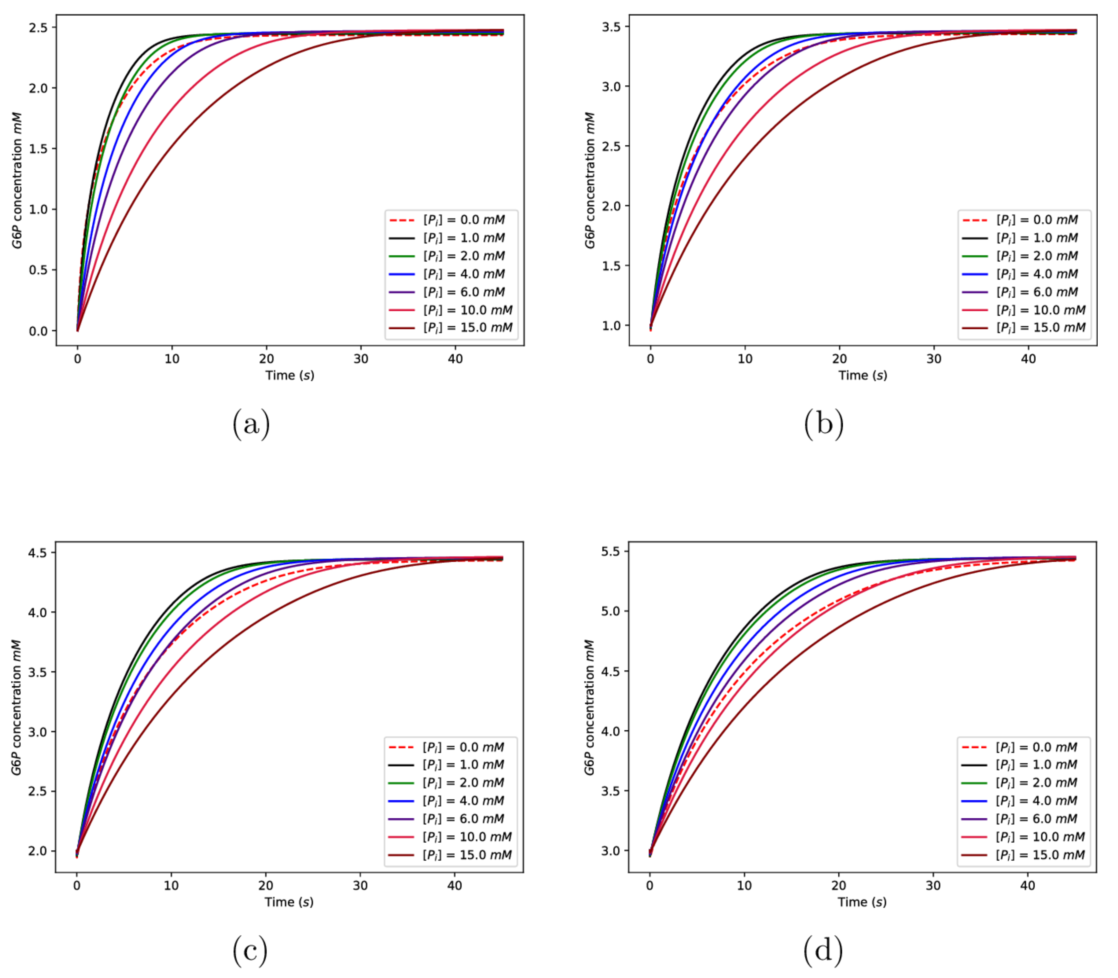
Figure 8 shows the time evolution of the concentration of $G6P$ for a range of different initial concentrations of $P_i$ and $G6P$. In the numerical results displayed here, the initial concentration of glucose was taken to be 2.5 mM [54], and the total concentration of the enzyme was taken to be $6.65\times {10}^{-2}$ mM [53]. We begin by noting some broad features of the behaviour exhibited in Figure 8. All of the curves are increasing functions of time, as would be expected since $G6P$ levels increase as the available glucose is phosphorylated. The levelling off of the curves corresponds to the exhaustion of the available glucose substrate. It is also noteworthy that the time scale over which the phosphorylation process was completed was of the order of ten seconds, a prediction that is consistent with the literature values [61,62].

In Figure 8, Subplots (a), (b), (c), and (d) correspond to differing initial concentrations of $G6P$, with (a) having the lowest initial concentration and (d) the highest. It is clear that the time for the phosphorylation process to be completed increased with increasing initial concentration of $G6P$. This again was as expected since $G6P$ is the species that is responsible for both the allosteric and competitive product inhibition of the enzyme, and so increasing its concentration should slow the phosphorylation process.

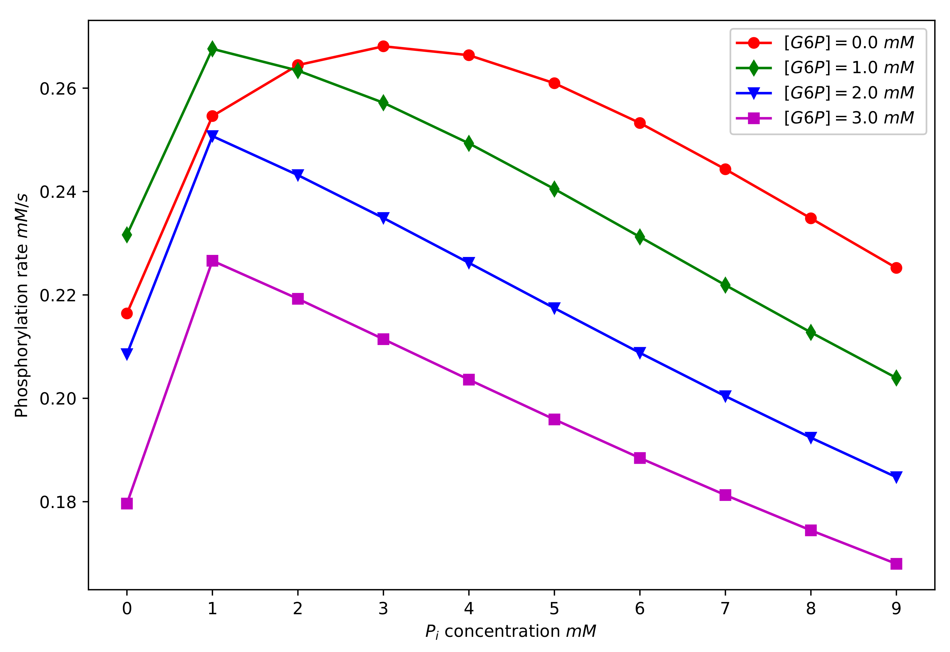
The dependence of the phosphorylation behaviour on the initial concentration of inorganic phosphate is more subtle and interesting. Focus, for example, on the subplot Figure 8d, and begin by considering the curve corresponding to $\left[P_i\right]=0$. This is the curve corresponding to zero initial $P_i$ concentration, and it gives a convenient reference. We note that for relatively low $P_i$ concentrations (1 mM, 2 mM), the phosphorylation process was faster than the phosphate-free case. However, for the higher concentrations ($P_i\ge 10$ mM), we note that the phosphorylation rate was slower relative to the phosphate free case. This is in line with experimental findings [4,11,41], which showed that for low concentrations of phosphate (few millimolar), enzyme inhibition by $G6P$ is antagonised and that for higher phosphate concentrations, enzyme activity is inhibited. In the context of the current modelling, this behaviour is explained by recalling that for low concentrations of $P_i$, the higher affinity N-binding site for $P_i$ dominates and inhibition by $G6P$ is antagonised. However, for higher $P_i$ concentrations, $P_i$ binding to the lower affinity C-site is significant and enzyme activity is inhibited. This phenomenon is clearly exhibited in Figure 9, where we show plots of the phosphorylation rate as a function of inorganic phosphate $P_i$ concentration and for four different initial concentrations of $G6P$.

3.2. Results of the Global Sensitivity Analysis

The Sobol global sensitivity analysis employed in the current study was described in the Methods Section, and it was implemented using the SALib package [59]. A Sobol analysis enabled us to quantify how variations in the model parameters:

$$\mathbf{p}=(k_{-G6}^P,k_{-P},k^{-P},k_{-G6},k^{-G6},k_{-T},k^{-T},k_{-G},k^{-G},k_0,k^G,k_G,k^T,k_T,k^{G6},k_{G6},k^P,k_P,k_{G6}^P)$$

affect the model output. The parameters here are the model rate constants and are described in Table 2. The model is of the form $\mathbf{y}=\mathbf{f}(\mathbf{p},t)$, where the inputs are the parameters $\mathbf{p}$ and the time t, and the output $\mathbf{y}$ gives the predictions for the concentrations of the model species at time t. In the current study, we confined our attention to the output for the $G6P$ concentration since $G6P$ is the product here.

Default settings for the SALib package were used, with one exception: no second-order indices were calculated [59]. We calculated first-order and total sensitivity indices for the times $t=2,4,6,8,10$ s. The output was then $G6P(t=2,4,6,8,10 \mathrm{s})$, and the purpose of the analysis was to evaluate the sensitivity of this output to variations in the parameters using the sensitivity indices. The $G6P$ values were calculated by numerically integrating the governing ordinary differential equations, as previously described. The initial concentration for $G6P$ was taken to be $2.0$ mM when numerically integrating the differential equations. Two choices for the initial concentration of phosphate were made, $2.0$ mM (low $P_i$ concentration) and $10.0$ mM (high $P_i$ concentration). The initial concentrations for the enzyme, glucose, and $ATP$ are given in Table 3. The remaining species had zero initial concentration.

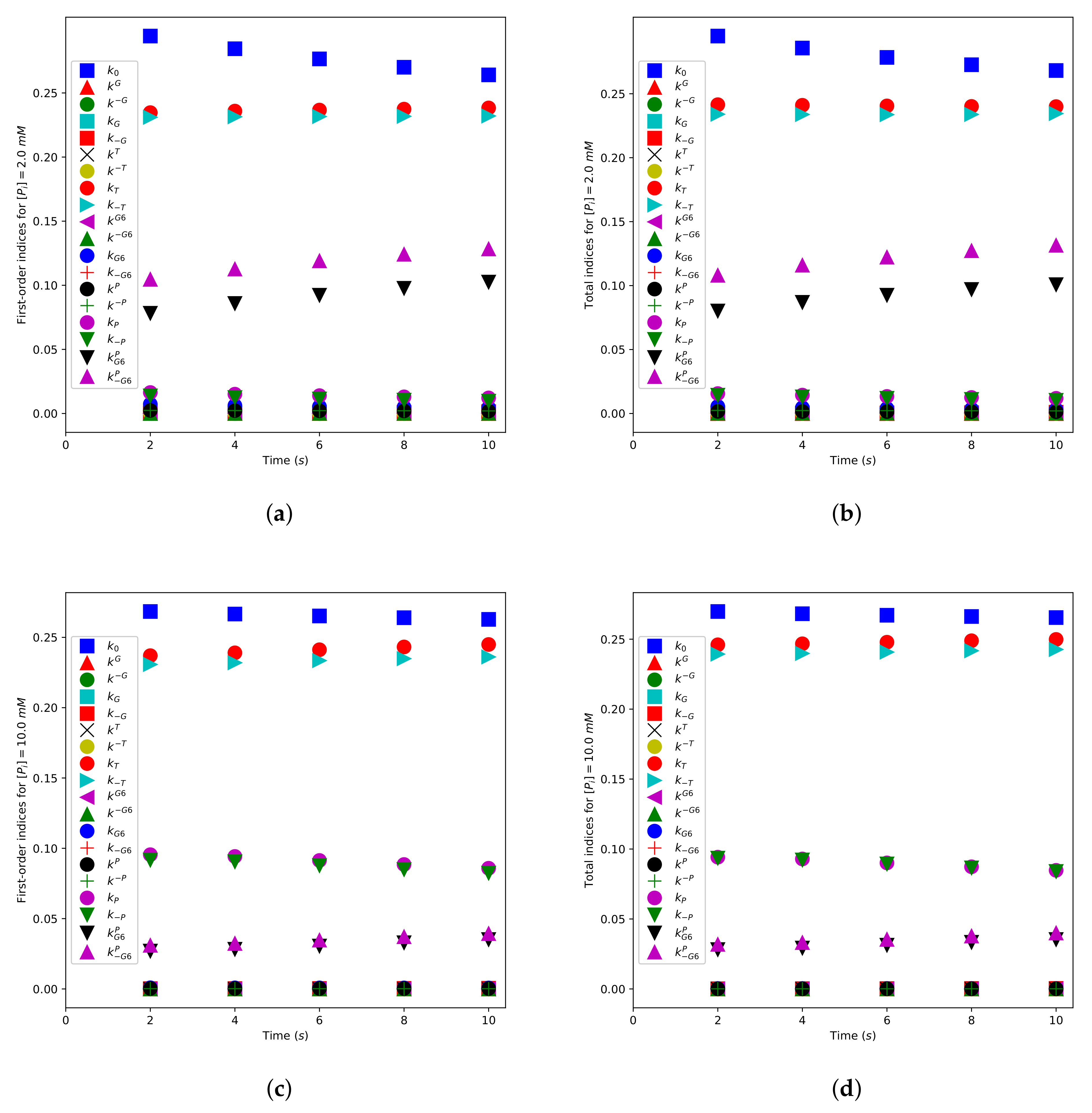
Figure 10 displays first-order sensitivity indices and total sensitivity indices for the model parameters. Figure 10a,b shows values for a low initial phosphate concentration ($2.0$ mM), while Figure 10c,d gives values for a high initial phosphate concentration ($10.0$ mM). For convenience, we split the model parameters into three groups: Group I: $k^G$, $k^{-G}$, $k_G$, $k_{-G}$, $k^T$, $k^{-T}$, $k^{G6}$, $k^{-G6}$, $k_{G6}$, $k_{-G6}$, $k^P$, $k^{-P}$, Group II: $k_P$, $k_{-P}$, and Group III: $k_0$, $k_T$, $k_{-T}$, $k_{G6}^P$, $k_{-G6}^P$. The sensitivity indices for all of the Group I parameters are small. This means that the rate of $G6P$ production is relatively insensitive to modest variations in the assumed values of these parameters. The parameters in Group I describe, among other things, the rate of binding and unbinding of glucose to both the N- and the C-domains of the enzyme and the rate of binding/unbinding of $P_i$ to the N-domain of the enzyme.

We now turn our attention to the parameters in Group III. The first-order sensitivity indices for all of these parameters are relatively large, implying that the $G6P$ production rate is relatively sensitive to variations in the assumed values of these parameters. The Group III parameters determine the turnover rate of the enzyme, the rate of binding/unbinding of $ATP$ to the C- domain of the enzyme, and the rate of binding/unbinding of $G6P$ to the C-domain of the enzyme when a $P_i$ molecule is bound at its N-site. It is noteworthy that the indices $S_9$ and $S_{-9}$ are quite sensitive to the phosphate concentration, being significantly larger for lower initial phosphate concentration. Hence, for low phosphate concentrations, the binding of $P_i$ to the N-binding site is one of the key regulators of enzyme activity.

The parameters for Group II ($k_{-P}$, $k_P$) are also seen to be sensitive to the phosphate concentration, being small for the low phosphate cases and significant for higher phosphate cases. These parameters determine the rate of binding/unbinding of $P_i$ to its C-binding site.

It is clear from Figure 10 that the first-order sensitivity indices are close to the total sensitivity indices. Hence, interactions between any of the parameters $k_i$ and the other model parameters do not significantly affect the model output.

3.3. Further Numerical Results

We now display some further numerical solutions inspired by the results of the sensitivity analysis just presented. In these calculations, the default values used for the k parameters are given in Table 2, and the initial concentrations for the enzyme, glucose and $ATP$ are given in Table 3. The initial concentrations of $G6P$ and $P_i$ were taken to be 3 mM and 6 mM, respectively, corresponding to a high phosphate concentration case.

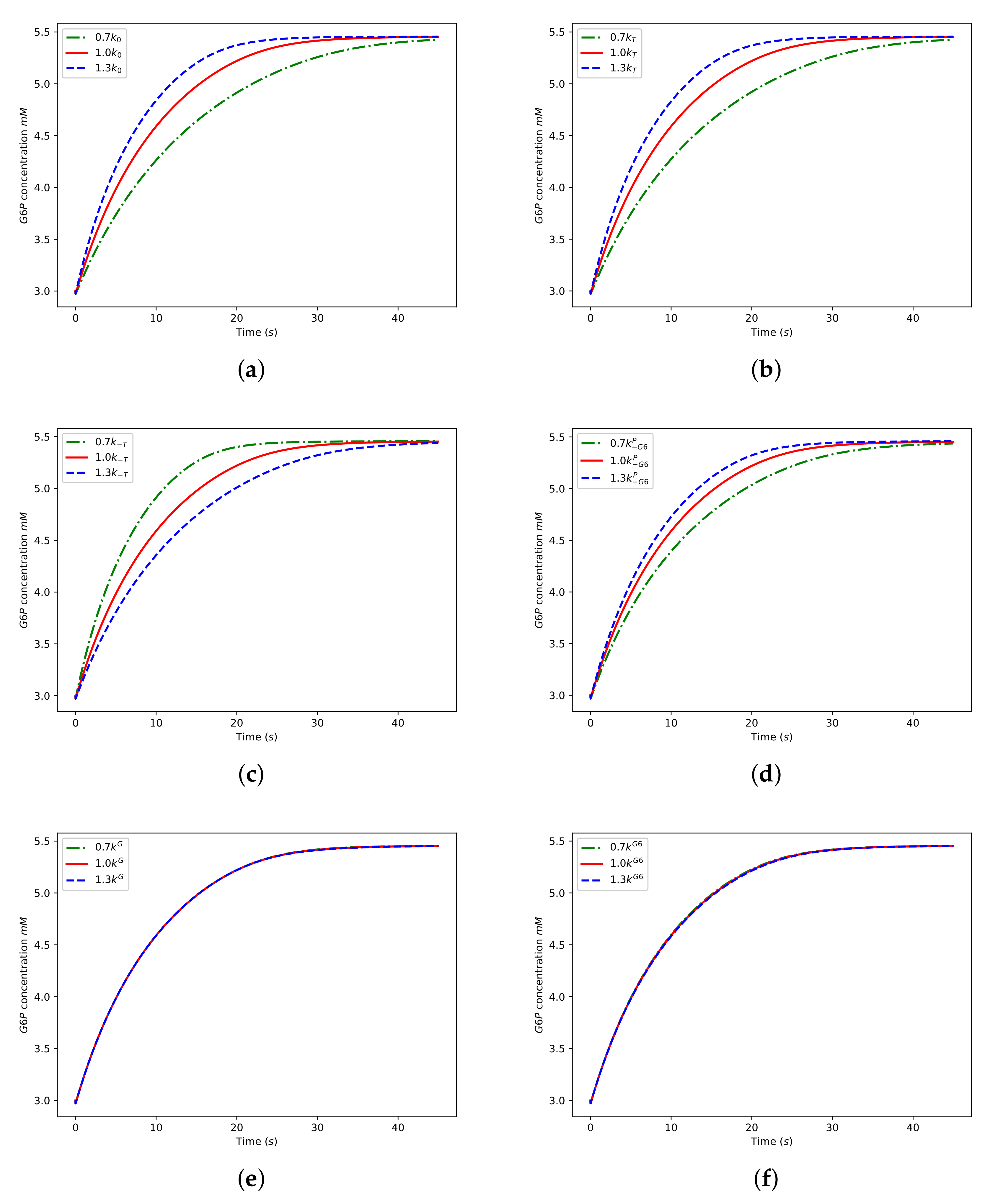
We illustrate how the new numerical results shown in Figure 11 were generated by considering a particular example. Consider the curves displayed in Figure 11a. The solid red curve was generated using the default values for the k parameters. The dashed blue curve was generated using the default values, except that $1.3k_0$ was used rather than $k_0$, and the dash-dotted green curve was generated using $0.7k_0$ rather than $k_0$. Hence, the three curves shown in Figure 11a help evaluate the sensitivity of the model output to variations in the parameter $k_0$. The remaining subplots in Figure 11 were generated by repeating this process for the parameters $k_T$, $k_{-T}$, $k_{-G6}^P$, $k^G$, and $k^{G6}$.

The results shown in Figure 11 are consistent with the predictions of the sensitivity analysis since the model output is seen to be quite sensitive to the parameters with relatively large sensitivity indices ($k_0$, $k_T$, $k_{-T}$, $k_{-G6}^P$), but insensitive to the parameters with small indices ($k^G$, $k^{G6}$).

3.4. Model Reduction

Motivated by the results of the sensitivity analysis, we now consider a simplified model (SM). This model was obtained from the full model by setting:

$$k^G=k^{-G}=k^T=k^{-T}=0.$$

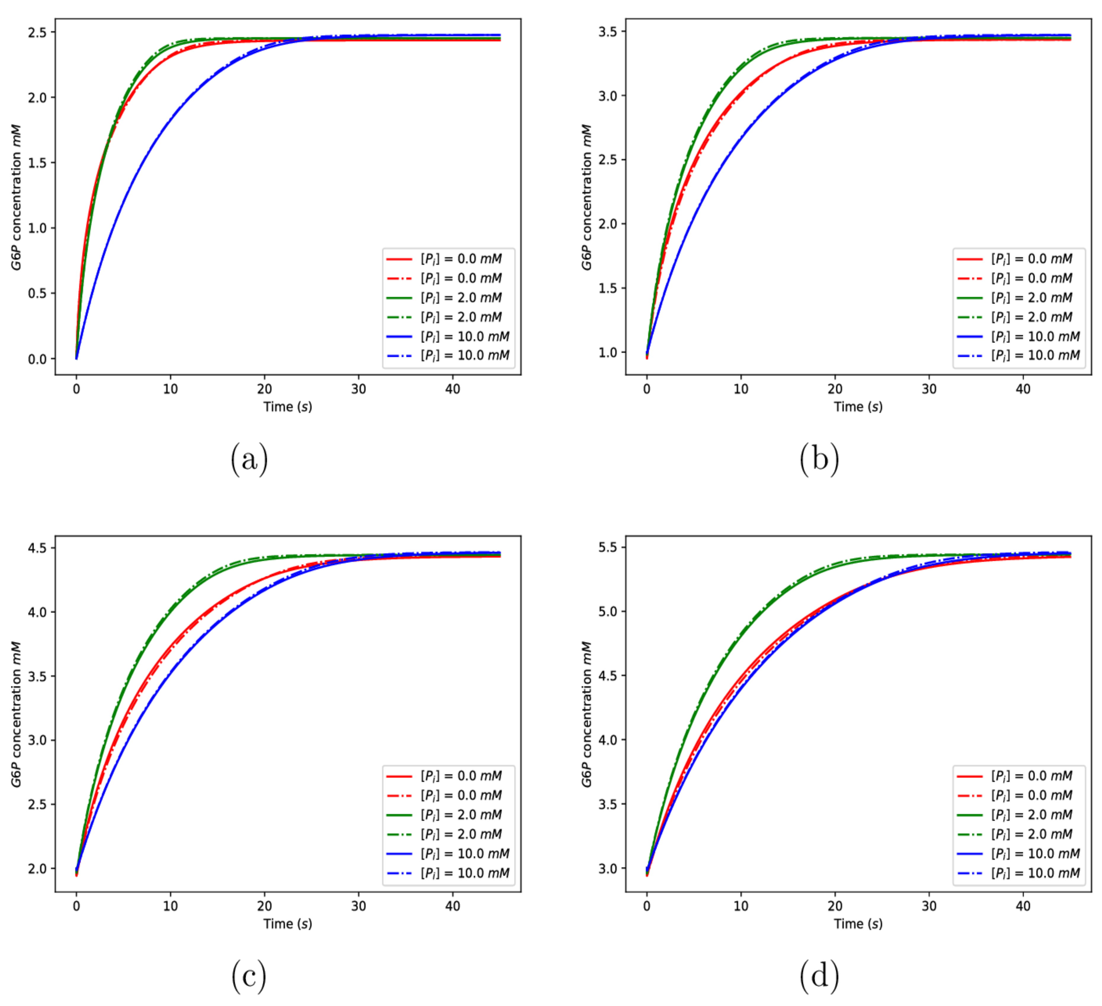
In this SM, glucose molecules do not bind to their N-domain site and $ATP$ molecules do not bind to their N-domain site. This reduction removes 46 chemical reactions from the model system and reduces the number of governing equations by 24. We previously saw that the sensitivity indices for all of these parameters are small, and so we anticipated that the output for these models should typically closely match that for the full model. The initial conditions used to generate the numerical solutions for the SM were the same as those used for the full model, with the exception of the initial conditions for $G6P$ and $P_i$, which are specified on the numerical figures. Figure 12 compares solutions of the full model with solutions of the SM, where solid curves are solutions to the full model and dashed-dotted curves are solutions to the SM.

It is seen in Figure 12 that the results of the full model and the SM are close in all cases, suggesting that the full model may reasonably be simplified by dropping the mechanisms of glucose and $ATP$ binding to the N-domains.

4. Conclusions

In this paper, we developed a comprehensive mathematical model describing the phosphorylation of glucose by the enzyme hexokinase I. Glucose phosphorylation is the first step of the glycolysis pathway, and so, it is carefully regulated by cells. The regulation of hexokinase I is quite complex and includes three inhibitory mechanisms: a competitive product inhibitory mechanism, an allosteric product inhibitory mechanism, and a competitive inhibitory mechanism. We used the mathematical model to help unpack the regulatory behaviour of hexokinase I. We make the following remarks:

• Model novelty: The biological evidence underpinning the modelling developed here has been established elsewhere. Nevertheless, the current study represents the first time that these ideas have been synthesised into a detailed mathematical model. The model incorporates numerous bound states for the enzyme, together with their associated activation status; the potential practical significance of this from the point of view of experimental work is explained in the next point. It is also noteworthy that the current modelling does not make any equilibrium assumptions;
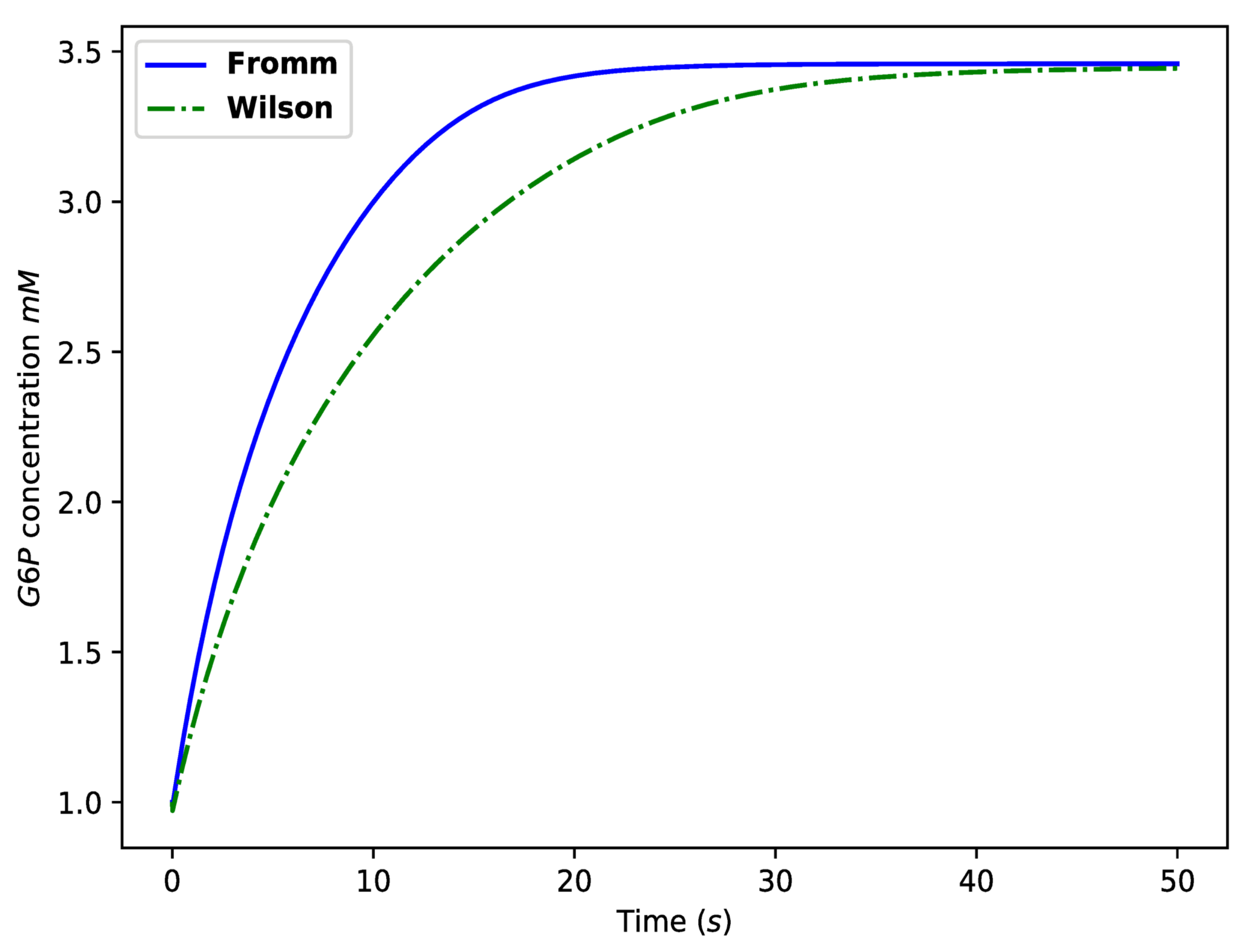
• The mathematical model and experimental data: The model presented here may be of particular value when combined with an appropriate in vitro experimental approach. In particular, the mathematical model may aid in identifying the correct biological mechanism from amongst a set of competing biological mechanisms. For example, two competing models for the function of hexokinase I are the Fromm model and the Wilson model, as described in Chapter III of [63]. Since the model developed here is sufficiently refined, both suggestions may be simulated by choosing appropriate parameter values in the model. Comparing both simulated curves with appropriate experimental data may assist in selecting the correct mechanism; see Figure 13;
• Biological insight: The model was numerically integrated using the SciPy Python library, and the solutions obtained were found to be consistent with the known behaviour of hexokinase I. The simulations also provided biological insights into subtle aspects of the enzyme behaviour, such as the dependence of the phosphorylation rate on the concentration of inorganic phosphate or the concentration of the enzyme product $G6P$. Further insight was obtained by carrying out a global sensitivity analysis, which revealed the key mechanisms of hexokinase I regulation. The results of this analysis showed that the rate of phosphorylation is sensitive to the following factors: the turnover rate of the enzyme; the rate of binding/unbinding of $ATP$ to/from the C-domain of the enzyme; the rate of binding/unbinding of $G6P$ to/from the C-domain of the enzyme with a $P_i$ molecule bound at the N-domain for low phosphate concentration; and the rate of binding/unbinding of phosphate to/from the C-domain of the enzyme for high phosphate concentration;
• Simplified model: One reduced model was developed based on the results of the sensitivity analysis. This simpler model produced results that closely matched the results of the full model;
• Software. The software developed in this study to numerically integrate the governing equations and to implement the sensitivity analysis has been made available in the Supplementary Material and online (https://github.com/vinh-mai/Hexokinase-2019 accessed on 1 August 2021).

Although the model developed in the current study is comprehensive and detailed, there is scope for improvement and future work. For example, one avenue for future research is to incorporate the full detail of the Bi Bi mechanism in the modelling. Furthermore, glucose-6-phosphate binding to its N-binding site not only allosterically inhibits the enzyme, but also stimulates enzyme release from mitochondria [64,65], and the incorporation of this effect provides another interesting avenue for future study. Finally, the possible inhibition of hexokinase I by $ADP$ [51] was not explored in the current study.

References

- Rehberg, M.; Ritter, J.B.; Reichl, U. Glycolysis is governed by growth regime and simple enzyme regulation in adherent MDCK cells. PLoS Comput. Biol. 2014, 10, e1003885. [Google Scholar] [CrossRef] [PubMed] [Green Version]
- Katzen, H.M.; Schimke, R.T. Multiple forms of hexokinase in the rat: Tissue distribution, age dependency, and properties. Proc. Natl. Acad. Sci. USA 1965, 54, 1218–1225. [Google Scholar] [CrossRef] [Green Version]
- Stocchi, V.; Magnani, M.; Canestrari, F.; Dacha, M.; Fornaini, G. Multiple forms of human red blood cell hexokinase. Preparation, characterization, and age dependence. J. Biol. Chem. 1982, 257, 2357–2364. [Google Scholar] [CrossRef]
- Wilson, J. Hexokinases. Rev. Physiol. Biochem. Pharmacol. 1995, 126, 65. [Google Scholar]
- Lowry, O.H.; Passonneau, J.V. The relationships between substrates and enzymes of glycolysis in brain. J. Biol. Chem. 1964, 239, 31–42. [Google Scholar] [CrossRef]
- Rapoport, S. The regulation of glycolysis in mammalian erythrocytes. Essays Biochem. 1968, 4, 69–103. [Google Scholar]
- Ritov, V.B.; Kelley, D.E. Hexokinase isozyme distribution in human skeletal muscle. Diabetes 2001, 50, 1253–1262. [Google Scholar] [CrossRef] [PubMed] [Green Version]
- Heikkinen, S.; Suppola, S.; Malkki, M.; Deeb, S.S.; Jänne, J.; Laakso, M. Mouse hexokinase II gene: Structure, cDNA, promoter analysis, and expression pattern. Mamm. Genome 2000, 11, 91–96. [Google Scholar] [CrossRef]
- Sebastian, S.; Edassery, S.; Wilson, J.E. The human gene for the type III isozyme of hexokinase: Structure, basal promoter, and evolution. Arch. Biochem. Biophys. 2001, 395, 113–120. [Google Scholar] [CrossRef]
- Cardenas, M.L.; Cornish-Bowden, A.; Ureta, T. Evolution and regulatory role of the hexokinases. Biochim. Biophys. Acta (BBA)-Mol. Cell Res. 1998, 1401, 242–264. [Google Scholar] [CrossRef] [Green Version]
- Wilson, J.E. Isozymes of mammalian hexokinase: Structure, subcellular localization and metabolic function. J. Exp. Biol. 2003, 206, 2049–2057. [Google Scholar] [CrossRef] [Green Version]
- Iynedjian, P.B. Mammalian glucokinase and its gene. Biochem. J. 1993, 293, 1. [Google Scholar] [CrossRef]
- Printz, R.L.; Magnuson, M.A.; Granner, D.K. Mammalian glucokinase. Annu. Rev. Nutr. 1993, 13, 463–496. [Google Scholar] [CrossRef] [PubMed]
- Beutler, E. Disorders due to enzyme defects in the red blood cell. Adv. Metab. Disord. 1972, 6, 131–160. [Google Scholar]
- Bianchi, M.; Crinelli, R.; Serafini, G.; Giammarini, C.; Magnani, M. Molecular bases of hexokinase deficiency. Biochim. Biophys. Acta (BBA)-Mol. Basis Dis. 1997, 1360, 211–221. [Google Scholar] [CrossRef] [Green Version]
- Becker, T.C.; BeltrandelRio, H.; Noel, R.J.; Johnson, J.H.; Newgard, C.B. Overexpression of hexokinase I in isolated islets of Langerhans via recombinant adenovirus. Enhancement of glucose metabolism and insulin secretion at basal but not stimulatory glucose levels. J. Biol. Chem. 1994, 269, 21234–21238. [Google Scholar] [CrossRef]
- Pan, M.; Han, Y.; Basu, A.; Dai, A.; Si, R.; Willson, C.; Balistrieri, A.; Scott, B.T.; Makino, A. Overexpression of hexokinase 2 reduces mitochondrial calcium overload in coronary endothelial cells of type 2 diabetic mice. Am. J. Physiol.-Cell Physiol. 2018, 314, C732–C740. [Google Scholar] [CrossRef]
- Azoulay-Zohar, H.; Israelson, A.; Salah, A.H.; Shoshan-Barmatz, V. In self-defence: Hexokinase promotes voltage-dependent anion channel closure and prevents mitochondria-mediated apoptotic cell death. Biochem. J. 2004, 377, 347–355. [Google Scholar] [CrossRef]
- Halestrap, A.P.; McStay, G.P.; Clarke, S.J. The permeability transition pore complex: Another view. Biochimie 2002, 84, 153–166. [Google Scholar] [CrossRef]
- Preller, A.; Wilson, J.E. Localization of the type III isozyme of hexokinase at the nuclear periphery. Arch. Biochem. Biophys. 1992, 294, 482–492. [Google Scholar] [CrossRef]
- Wyatt, E.; Wu, R.; Rabeh, W.; Park, H.W.; Ghanefar, M.; Ardehali, H. Regulation and cytoprotective role of hexokinase III. PLoS ONE 2010, 5, e13823. [Google Scholar] [CrossRef] [PubMed] [Green Version]
- Iynedjian, P. Molecular physiology of mammalian glucokinase. Cell. Mol. Life Sci. 2009, 66, 27. [Google Scholar] [CrossRef] [PubMed] [Green Version]
- White, T.K.; Wilson, J.E. Isolation and characterization of the discrete N-and C-terminal halves of rat brain hexokinase: Retention of full catalytic activity in the isolated C-terminal half. Arch. Biochem. Biophys. 1989, 274, 375–393. [Google Scholar] [CrossRef]
- Arora, K.K.; Filburn, C.R.; Pedersen, P.L. Structure/function relationships in hexokinase. Site-directed mutational analyses and characterization of overexpressed fragments implicate different functions for the N-and C-terminal halves of the enzyme. J. Biol. Chem. 1993, 268, 18259–18266. [Google Scholar] [CrossRef]
- Zeng, C.; Fromm, H.J. Active site residues of human brain hexokinase as studied by site-specific mutagenesis. J. Biol. Chem. 1995, 270, 10509–10513. [Google Scholar] [CrossRef] [PubMed] [Green Version]
- Ardehali, H.; Printz, R.L.; Whitesell, R.R.; May, J.M.; Granner, D.K. Functional interaction between the N-and C-terminal halves of human hexokinase II. J. Biol. Chem. 1999, 274, 15986–15989. [Google Scholar] [CrossRef] [Green Version]
- Ardehali, H.; Yano, Y.; Printz, R.L.; Koch, S.; Whitesell, R.R.; May, J.M.; Granner, D.K. Functional Organization of Mammalian Hexokinase II retention of catalytic and regulatory functions in both the NH- and COOH-terminal halves. J. Biol. Chem. 1996, 271, 1849–1852. [Google Scholar] [CrossRef] [Green Version]
- Schirch, D.M.; Wilson, J.E. Rat brain hexokinase: Location of the substrate hexose binding site in a structural domain at the C-terminus of the enzyme. Arch. Biochem. Biophys. 1987, 254, 385–396. [Google Scholar] [CrossRef]
- Tsai, H.J.; Wilson, J.E. Functional organization of mammalian hexokinases: Characterization of the rat type III isozyme and its chimeric forms, constructed with the N-and C-terminal halves of the type I and type II isozymes. Arch. Biochem. Biophys. 1997, 338, 183–192. [Google Scholar] [CrossRef]
- Tsai, H.J. Functional organization and evolution of mammalian hexokinases: Mutations that caused the loss of catalytic activity in N-terminal halves of type I and type III isozymes. Arch. Biochem. Biophys. 1999, 369, 149–156. [Google Scholar] [CrossRef]
- Ning, J.; Purich, D.L.; Fromm, H.J. Studies on the kinetic mechanism and allosteric nature of bovine brain hexokinase. J. Biol. Chem. 1969, 244, 3840–3846. [Google Scholar] [CrossRef]
- Gerber, G.; Preissler, H.; Heinrich, R.; Rapoport, S.M. Hexokinase of human erythrocytes: Purification, kinetic model and its application to the conditions in the cell. Eur. J. Biochem. 1974, 45, 39–52. [Google Scholar] [CrossRef] [PubMed]
- Purich, D.L.; Fromm, H.J. The kinetics and regulation of rat brain hexokinase. J. Biol. Chem. 1971, 246, 3456–3463. [Google Scholar] [CrossRef]
- Wilson, J.E. Brain hexokinase, the prototype ambiquitous enzyme. In Current Topics in Cellular Regulation; Elsevier: Amsterdam, The Netherlands, 1980; Volume 16, pp. 1–44. [Google Scholar]
- Rudolph, F.B.; Fromm, H.J. Computer simulation studies with yeast hexokinase and additional evidence for the random Bi Bi mechanism. J. Biol. Chem. 1971, 246, 6611–6619. [Google Scholar] [CrossRef]
- Rosano, C.; Sabini, E.; Rizzi, M.; Deriu, D.; Murshudov, G.; Bianchi, M.; Serafini, G.; Magnani, M.; Bolognesi, M. Binding of non-catalytic ATP to human hexokinase I highlights the structural components for enzyme–membrane association control. Structure 1999, 7, 1427–1437. [Google Scholar] [CrossRef] [Green Version]
- Liu, X.; Kim, C.S.; Kurbanov, F.T.; Honzatko, R.B.; Fromm, H.J. Dual mechanisms for glucose 6-phosphate inhibition of human brain hexokinase. J. Biol. Chem. 1999, 274, 31155–31159. [Google Scholar] [CrossRef] [Green Version]
- Sebastian, S.; Wilson, J.E.; Mulichak, A.; Garavito, R.M. Allosteric regulation of type I hexokinase: A site-directed mutational study indicating location of the functional glucose 6-phosphate binding site in the N-terminal half of the enzyme. Arch. Biochem. Biophys. 1999, 362, 203–210. [Google Scholar] [CrossRef]
- Fang, T.Y.; Alechina, O.; Aleshin, A.E.; Fromm, H.J.; Honzatko, R.B. Identification of a phosphate regulatory site and a low affinity binding site for glucose 6-phosphate in the N-terminal half of human brain hexokinase. J. Biol. Chem. 1998, 273, 19548–19553. [Google Scholar] [CrossRef] [Green Version]
- Lazo, P.; Sols, A.; Wilson, J. Brain hexokinase has two spatially discrete sites for binding of glucose-6-phosphate. J. Biol. Chem. 1980, 255, 7548–7551. [Google Scholar] [CrossRef]
- Ellison, W.R.; Lueck, J.; Fromm, H. Studies on the mechanism of orthophosphate regulation of bovine brain hexokinase. J. Biol. Chem. 1975, 250, 1864–1871. [Google Scholar] [CrossRef]
- Aleshin, A.E.; Zeng, C.; Bourenkov, G.P.; Bartunik, H.D.; Fromm, H.J.; Honzatko, R.B. The mechanism of regulation of hexokinase: New insights from the crystal structure of recombinant human brain hexokinase complexed with glucose and glucose-6-phosphate. Structure 1998, 6, 39–50. [Google Scholar] [CrossRef]
- Lubert, S.; John, L.T.; Jeremy, M.B. Biochemistry, 5th ed.; WH Freeman: New York, NY, USA, 2002. [Google Scholar]
- Liu, J.; Nussinov, R. Allostery: An overview of its history, concepts, methods, and applications. PLoS Comput. Biol. 2016, 12, e1004966. [Google Scholar] [CrossRef]
- Voit, E.O.; Martens, H.A.; Omholt, S.W. 150 years of the mass action law. PLoS Comput. Biol. 2015, 11, e1004012. [Google Scholar] [CrossRef] [Green Version]
- Taylor, K.B. Enzyme Kinetics and Mechanisms; Springer Science & Business Media: Berlin/Heidelberg, Germany, 2002; Volume 64. [Google Scholar]
- Python Software Foundation. Available online: https://www.python.org/ (accessed on 19 April 2019).
- SciPy Open Source Python Library. Available online: https://www.scipy.org/ (accessed on 19 April 2019).
- The Odeint Solver in the Integrate Module of the SciPy Library. Available online: https://docs.scipy.org/doc/scipy/reference/generated/scipy.integrate.odeint.html (accessed on 19 April 2019).
- The LDOSA Program in the FORTRAN Library Odepack. Available online: http://www.oecd-nea.org/tools/abstract/detail/uscd1227 (accessed on 19 April 2019).
- Rijksen, G.; Staal, G.E. Regulation of human erythrocyte hexokinase: The influence of glycolytic intermediates and inorganic phosphate. Biochim. Biophys. Acta (BBA)-Enzymol. 1977, 485, 75–86. [Google Scholar] [CrossRef]
- Yang, C.R.; Shapiro, B.E.; Mjolsness, E.D.; Hatfield, G.W. An enzyme mechanism language for the mathematical modeling of metabolic pathways. Bioinformatics 2004, 21, 774–780. [Google Scholar] [CrossRef] [Green Version]
- Segel, I.H. Enzyme Kinetics: Behavior and Analysis of Rapid Equilibrium and Steady State Enzyme Systems; Wiley: New York, NY, USA, 1975. [Google Scholar]
- Foley, J.E.; Cushman, S.W.; Salans, L.B. Intracellular glucose concentration in small and large rat adipose cells. Am. J. Physiol.-Endocrinol. Metab. 1980, 238, E180–E185. [Google Scholar] [CrossRef] [PubMed]
- Wilson, J.E. Brain hexokinase a proposed relation between soluble-particulate distribution and activity in vivo. J. Biol. Chem. 1968, 243, 3640–3647. [Google Scholar] [CrossRef]
- Sobol, I.M. Global sensitivity indices for nonlinear mathematical models and their Monte Carlo estimates. Math. Comput. Simul. 2001, 55, 271–280. [Google Scholar] [CrossRef]
- Saltelli, A.; Ratto, M.; Andres, T.; Campolongo, F.; Cariboni, J.; Gatelli, D.; Saisana, M.; Tarantola, S. Global Sensitivity Analysis: The Primer; John Wiley & Sons: Hoboken, NJ, USA, 2008. [Google Scholar]
- Mai, V.Q.; Vo, T.T.; Meere, M. Modelling hyaluronan degradation by streptococcus pneumoniae hyaluronate lyase. Math. Biosci. 2018, 303, 126–138. [Google Scholar] [CrossRef] [PubMed]
- Herman, J.; Usher, W. SALib: An open-source Python library for sensitivity analysis. J. Open Source Softw. 2017, 2. [Google Scholar] [CrossRef]
- Sensitivity Analysis Library for Systems Modeling. Available online: https://github.com/SALib (accessed on 19 April 2019).
- Milo, R.; Phillips, R. Cell Biology by the Numbers; Garland Science: New York, NY, USA, 2015. [Google Scholar]
- John, S.; Weiss, J.N.; Ribalet, B. Subcellular localization of hexokinases I and II directs the metabolic fate of glucose. PLoS ONE 2011, 6, e17674. [Google Scholar] [CrossRef] [Green Version]
- Shen, L. Allosteric Mechanisms in Recombinant Human Hexokinase Type I. Ph.D. Thesis, Iowa State University, Ames, IA, USA, 2012. [Google Scholar]
- Skaff, D.A.; Kim, C.S.; Tsai, H.J.; Honzatko, R.B.; Fromm, H.J. Glucose 6-phosphate release of wild-type and mutant human brain hexokinases from mitochondria. J. Biol. Chem. 2005, 280, 38403–38409. [Google Scholar] [CrossRef] [Green Version]
- Rose, I.A.; Warms, J.V. Mitochondrial hexokinase release, rebinding, and location. J. Biol. Chem. 1967, 242, 1635–1645. [Google Scholar] [CrossRef]
Figure 1.
Schematic representations for hexokinase, glucose, glucose-6-phosphate, adenosine triphosphate (), adenosine diphosphate (), and inorganic phosphate (). (a) The hexokinase I enzyme. The C- and N-domains are coloured green and light blue, respectively. ⊔: binding sites for glucose; ∨: binding sites for , , and . (b) Glucose. (c) Glucose-6-phosphate. (d) Adenosine triphosphate (). (e) Adenosine diphosphate (). (f) Inorganic phosphate ().
Figure 2.
The Bi Bi mechanism for hexokinase I. Here, E, A, B, C, and D represent the hexokinase enzyme, , glucose, , and , respectively. and are the dissociation constants for .
Figure 3.
The eight possible configurations of a hexokinase molecule where only one of the binding sites is occupied. Figures (a–e) depict active states for the enzyme, while (f–h) depict inactive states. (a) An molecule bound to the N-domain. (b) An molecule bound to the C-domain. (c) A glucose molecule bound to the N-domain. (d) A glucose molecule bound to the C-domain. (e) A molecule bound to the N-domain. (f) A molecule bound to the C-domain (competitive inhibition). (g) A molecule bound to the N-domain (allosteric product inhibition). (h) A molecule bound to the C-domain (competitive product inhibition).
Figure 4.
The Bi Bi mechanism for glucose phosphorylation. (a) The full Bi Bi mechanism for the phosphorylation of glucose. (b) The simplified Bi Bi mechanism modelled in the current study.
Figure 5.
The mechanism for the phosphorylation of glucose by hexokinase I.
Figure 6.
Diagram of chemical reactions producing the product. There are eight such reaction types, and each of them forms one and one molecule (denoted by D) and either a free enzyme or an enzyme complex.
Figure 7.
Diagram of chemical reactions forming all complexes in the mixture. E, 0, 1, 2, and 3 represent the free enzyme, glucose, , , and molecules, respectively. The red lines refer to reversible reactions involving glucose binding; the blue: binding; the green: binding; the brown: binding. Letters E with a superscript(s) and/or subscript(s) denote complexes of the enzyme, for instance is a complex of the enzyme with one glucose and one molecule bound at the N-binding site, and one molecule bound at the C-binding site.
Figure 8.
Numerical solutions of the model equations. The graphs show the concentration of as a function of time for various initial concentrations of and . The initial concentrations for are given in the legends on the graphs, and the initial concentrations are given by (a) 0 mM, (b) 1.0 mM, (c) 2.0 mM, and (d) 3.0 mM. The remaining parameter values can be found in the main text.
Figure 9.
Plots of the phosphorylation rate as a function of the initial concentration of phosphate and for four different initial concentrations of . The parameter values used to generate these curves can be found in Table 2 and Table 3. We note an initial increase in the phosphorylation rate in all cases, followed by a subsequent decrease in the rate. This is discussed further in the main text.
Figure 10.
Results of the global sensitivity analysis. (a) First-order sensitivity indices () and (b) total sensitivity indices () with mM. (c) First-order sensitivity indices and (d) total sensitivity indices with mM. The indices are calculated at the times . The remaining parameter values are given in the main body of the text.
Figure 11.
Numerical solutions of the model equations for a high level of . The graphs show the concentration of as a function of time, and the parameter values used can be found in the main body of the text. The solutions displayed help evaluate the sensitivity of the model output to the parameters (a) , (b) , (c) , (d) , (e) , and (f) .
Figure 12.
Comparison of the numerical solutions to the full model and the simplified model (SM). The solid curves are solutions to the full model, and the dashed-dotted curves are solutions to the SM. The initial concentrations for the phosphate are given on the figures, and the initial concentrations for are given by (a) 0 mM, (b) 1.0 mM, (c) 2.0 mM, and (d) 3.0 mM. The remaining parameter values used can be found in the main body of the text.
Figure 13.
An illustrative calculation comparing the predictions of the Wilson and Fromm models. Such calculations may assist experimental studies in identifying the correct model, as explained in the Conclusions Section. The Fromm model here is the model described in the current paper. The Wilson model is the same as the Fromm model except now can only bind to the N-binding site. The Fromm curve was generated using the parameter values displayed in Table 2 and Table 3 and initial concentrations mM, mM. The Wilson curve was generated using the same parameter values, except for s, mMs, s, s, 20,000 mMs, s, mMs, s.