
A Massively Parallel Hybrid Finite Volume/Finite Element Scheme for Computational Fluid Dynamics


1
Laboratory of Applied Mathematics, DICAM, University of Trento, Via Mesiano 77, 38123 Trento, Italy
2
Departamento de Matemática Aplicada a la Ingeniería Industrial, Universidad Politécnica de Madrid, José Gutierrez Abascal 2, 28006 Madrid, Spain
*
Authors to whom correspondence should be addressed.
Mathematics 2021, 9(18), 2316; https://0-doi-org.brum.beds.ac.uk/10.3390/math9182316
Submission received: 26 August 2021
/
Revised: 7 September 2021
/
Accepted: 9 September 2021
/
Published: 18 September 2021
(This article belongs to the Special Issue Modeling and Numerical Analysis of Energy and Environment 2021)
Abstract
:In this paper, we propose a novel family of semi-implicit hybrid finite volume/finite element schemes for computational fluid dynamics (CFD), in particular for the approximate solution of the incompressible and compressible Navier-Stokes equations, as well as for the shallow water equations on staggered unstructured meshes in two and three space dimensions. The key features of the method are the use of an edge-based/face-based staggered dual mesh for the discretization of the nonlinear convective terms at the aid of explicit high resolution Godunov-type finite volume schemes, while pressure terms are discretized implicitly using classical continuous Lagrange finite elements on the primal simplex mesh. The resulting pressure system is symmetric positive definite and can thus be very efficiently solved at the aid of classical Krylov subspace methods, such as a matrix-free conjugate gradient method. For the compressible Navier-Stokes equations, the schemes are by construction asymptotic preserving in the low Mach number limit of the equations, hence a consistent hybrid FV/FE method for the incompressible equations is retrieved. All parts of the algorithm can be efficiently parallelized, i.e., the explicit finite volume step as well as the matrix-vector product in the implicit pressure solver. Concerning parallel implementation, we employ the Message-Passing Interface (MPI) standard in combination with spatial domain decomposition based on the free software package METIS. To show the versatility of the proposed schemes, we present a wide range of applications, starting from environmental and geophysical flows, such as dambreak problems and natural convection, over direct numerical simulations of turbulent incompressible flows to high Mach number compressible flows with shock waves. An excellent agreement with exact analytical, numerical or experimental reference solutions is achieved in all cases. Most of the simulations are run with millions of degrees of freedom on thousands of CPU cores. We show strong scaling results for the hybrid FV/FE scheme applied to the 3D incompressible Navier-Stokes equations, using millions of degrees of freedom and up to 4096 CPU cores. The largest simulation shown in this paper is the well-known 3D Taylor-Green vortex benchmark run on 671 million tetrahedral elements on 32,768 CPU cores, showing clearly the suitability of the presented algorithm for the solution of large CFD problems on modern massively parallel distributed memory supercomputers.
Keywords:
incompressible and compressible Navier-Stokes equations; shallow water equations; finite element method; finite volume scheme; semi-implicit scheme on staggered unstructured meshes; ADER methodology; High-Performance Computing (HPC); Message-Passing Interface (MPI)MSC:
35L40; 65M08; 65M60; 65Y051. Introduction
Since the advent of modern computers and the first numerical methods for the approximate solution of nonlinear partial differential equations (PDE), the field of computational fluid dynamics (CFD) has been a major driving force for research and new developments in applied mathematics and scientific computing in the last decades, see (e.g., [1,2,3]) for the first finite difference schemes for CFD. Further groundbreaking inventions for the numerical solution of PDE are the finite element (FE) method, which makes use of discrete variational calculus, see (e.g., [4,5,6,7,8,9,10,11,12,13,14,15,16,17,18]), and finite volume (FV) schemes [19,20,21,22,23,24,25], which are based on the integral form of the governing PDE system. While finite element schemes are traditionally preferred for computational solid mechanics and stationary elliptic problems, finite volume schemes are widespread in the context of time-dependent hyperbolic partial differential equations, especially when flows become supersonic/supercritical and discontinuous solutions (shock waves) develop, see [26,27].
In [28,29,30,31], a novel family of semi-implicit hybrid FV/FE schemes has been developed and applied to incompressible, weakly compressible, and all Mach number flows, including shock waves. The main idea behind the hybrid FV/FE framework is a flux-vector splitting of the governing PDE system, see [32], where the purely convective (hyperbolic) terms are discretized with an explicit finite volume scheme, while the remaining pressure terms in the flux vector can be rewritten as a second order wave equation and are thus more conveniently discretized at the aid of an implicit finite element method. For the incompressible Navier-Stokes equations, the resulting pressure equation is indeed elliptic, hence the FE approach is clearly more convenient compared to a finite volume discretization. In order to avoid odd-even decoupling and checkerboard effects, the hybrid FV/FE method makes use of a staggered unstructured mesh, where the pressure field is defined in the vertices of a primal simplex mesh composed of triangles or tetrahedra, while all the other flow variables, such as density and momentum, are defined on a dual edge-based/face-based staggered dual mesh, see also [33,34,35]. The use of staggered meshes in CFD goes back to the pioneering work of Harlow and Welch [36] for the solution of the incompressible Navier-Stokes equations and was subsequently also employed, for example, in [37,38]. For a non-exhaustive overview of efficient semi-implicit schemes for CFD, see (e.g., [39,40,41,42,43,44,45,46,47,48,49,50,51,52,53]) and references therein.
In previous work on hybrid FV/FE schemes for the Navier-Stokes equations [28,29,30,31], all simulations have been performed with a classical sequential implementation, allowing the use of only one CPU core for a simulation, even on modern multi-core workstations. In order to reduce the computational cost and perform large simulations with complex geometries and fine meshes needed in CFD for aircraft and vehicles, see (e.g., [54,55,56,57,58]) and references therein for an overview, it is essential to use a parallel implementation. In this paper, the hybrid FV/FE scheme has been parallelized by using the Message-Passing Interface (MPI) standard. The computational domain is partitioned in space via the free domain decomposition software METIS [59], and each processor handles its own data and its own part of the computational domain, hence using a distributed data and distributed workload paradigm. While the parallelization of the explicit finite volume part is straightforward, the implicit discretization of the pressure terms leads to a very large and sparse linear algebraic system that needs to be solved. However, thanks to the underlying basic properties of the governing PDE and its finite element discretization, the resulting discrete pressure system is always symmetric and positive definite. An efficient parallel solution is therefore achieved at the aid of a matrix-free conjugate gradient (CG) method [60]. For more advanced and optimized linear solvers for finite elements, the reader is referred to [61,62,63,64]. The final structure of the matrix-vector product that needs to be evaluated in each CG iteration is similar to the one of an explicit method and can therefore be parallelized as usual at the aid of spatial domain decomposition. In this way, the computational cost is shared among all the processors, both for the explicit FV part as well as for the implicit FE part of the hybrid FV/FE scheme. The parallelism is achieved in all cases via the communication of data among neighboring MPI ranks via shadow/halo zones. For the efficient parallel implementation of explicit schemes for the solution of hyperbolic PDE, the reader is referred to [65,66,67,68,69,70], for example.
By using this parallel implementation of the hybrid FV/FE scheme, numerical simulations involving meshes with several hundreds of millions of elements can be run on modern massively parallel distributed memory supercomputers. Moreover, good parallel performance is obtained, as confirmed by a strong scaling analysis. The numerical solutions obtained with the parallel hybrid FV/FE scheme have been carefully compared with exact analytical, numerical and experimental reference solutions, obtaining in all cases a very good agreement. Currently, the algorithm presented in this paper is limited to simplex meshes, i.e., triangles in 2D and tetrahedra in 3D. Future work will concern the extension to mixed element unstructured meshes, including also prisms, pyramids, and hexahedra, as well as more general polygonal and polyhedral meshes, using e.g., the virtual element method (VEM), see [71,72,73] and references therein. Another limitation of the algorithm is the use of a pure MPI parallelization instead of a mixed MPI + OpenMP implementation.
The structure of this paper is as follows: The mathematical models and the underlying semi-discretization in time that is necessary for the semi-implicit hybrid FV/FE scheme are introduced in Section 2. In particular, the governing PDE systems solved in this paper are the incompressible, the weakly compressible, and the fully compressible Navier-Stokes equations, as well as the shallow water equations for geophysical free surface flows. The spatial discretization of the hybrid FV/FE scheme is presented in Section 3. Section 4 is devoted to describing the parallelization of the staggered semi-implicit hybrid FV/FE approach using the MPI standard. The performance of the parallel scheme is demonstrated via a quantitative speedup analysis. An extensive set of numerical results is presented in Section 5, ranging from the incompressible over the weakly compressible and fully compressible Navier-Stokes equations to the shallow water equations. The paper closes with some concluding remarks and an outlook to future work in Section 6.
2. Mathematical Models and Semi-Discretization in Time
In this section, we recall the mathematical models considered in this paper: the incompressible Navier-Stokes equations, the weakly compressible formulation of the Navier-Stokes equations in terms of the pressure, the fully compressible Navier-Stokes equations in terms of the total energy density, which are suitable for the description of all Mach number flows, and, last but not least, the shallow water equations for the modeling of geophysical free surface flows. Following the hybrid methodology proposed in [28,29,30,31,74], we rely on a flux vector splitting [32] of the associated semi-discrete systems in time. Consequently, we get a first set of transport-diffusion equations that can be efficiently discretized in space using classical explicit finite volume methods. The remaining set of equations can be expressed as a Poisson-type system in the case of the incompressible Navier-Stokes equations and as a second order wave equation for the pressure in the case of the compressible Navier-Stokes equations and the shallow water system. Continuous finite elements are used to solve this system due to the excellent mathematical properties they present for the solution of second order PDE in general and of elliptic problems in particular. Therefore, the corresponding weak formulation of the implicit pressure terms is presented for each mathematical model. Finally, we will recast the resulting systems into a general formulation easing the introduction of the spatial discretization of the equations in the next section.
2.1. Incompressible Navier-Stokes Equations
The incompressible Navier-Stokes equations read
where is the linear momentum, the density, the velocity vector, is the physical flux tensor related to the nonlinear convective terms in the momentum conservation equation, p denotes the pressure, and corresponds to the viscous stress tensor, which for laminar incompressible flows reads , with the dynamic viscosity.
Applying a projection method [53,75], to decouple the computation of the linear momentum unknowns and the pressure field, together with a semi-discretization in time of the above system yields
Throughout the paper, capital letters are used to identify discrete variables, i.e., is the discrete approximation of , while and so on. Intermediate variables are denoted with a tilde, e.g., is the intermediate variable for the linear momentum including all contributions needed to compute the solution at the new time step but for the spatial gradient of the pressure difference between the two consecutive times, . Besides, we denote with the computational domain and by its boundary, the outward-pointing normal vector, and by a test function. Then, Equations (4) and (5) can be seen as a Poisson-type problem with the following weak formulation:
Weak problem.
Find verifying
2.2. Weakly Compressible Flows
To develop a solver for weakly compressible flows, we consider the mass and momentum equations of the compressible Navier-Stokes system, combined with a pressure equation written in non-conservative form, see [30],
with the state vector and where is the flux related to the mass conservation equation, is the gravity vector, is the heat flux, the thermal conductivity coefficient, the temperature, and is the square of the isentropic sound speed c. Let us also note that the stress tensor for the laminar compressible regime reads , with the identity matrix, and for the ideal gas equation of state (EOS), we have , , with R the specific gas constant and the adiabatic index or ratio of specific heats.
Semi-discretization in time of the former system yields
with . The corresponding second order wave equation for the pressure, derived from (14) and (15), results in
Weak problem.
Find verifying
2.3. Compressible Navier-Stokes Equations for All Mach Number Flows
To get an all Mach number flow solver, we go back to the classical conservative formulation of the compressible Navier-Stokes equations in terms of the total energy density, [31],
Here, the state vector is .
To discretize the compressible system, we follow the flux splitting techniques introduced in [32,48], obtaining the following semi-discrete system in time:
where is the flux related to the kinetic energy. Let us remark that in (23)–(26), we have introduced a Picard iteration procedure, k the Picard index, in order to avoid the solution of a highly nonlinear pressure system, further details can be found in [31]. The weak formulation related to the pressure subsystem (23) reads
Weak problem.
Find verifying
2.4. Shallow Water Equations
Following [40], the well-known shallow water system of partial differential equations can be written as
where is the free surface elevation, h is the water depth, b is the bottom elevation, that we assume constant in time, is the conservative variable related to the velocity field, is the flux of the momentum conservation equation, g is the gravity constant, and is a shorthand notation for the bottom friction.
with the Strickler coefficient and n the Manning coefficient. An important aspect that should be noticed is that the hybrid FV/FE algorithm proposed is well balanced by construction so water at rest solutions are preserved [33,76,77].
After discretization in time and some manipulations of the resulting equations, see [74] for further details, we get
Similar to what we have already seen for the pressure subsystems for the compressible Navier-Stokes equations, we get a second order wave equation for the unknown free surface. Besides, to increase the accuracy in time, we employ the -method that reduces to the classical Crank-Nicolson scheme for . The final weak formulation results in
Weak problem.
Find verifying
In (34), we have introduced a new intermediate variable
2.5. General Formulation
As mentioned before, the former systems can be recast into a general formulation which eases the development of a general code for its solution. In particular, we consider two different sets of equations: the first one is related to the transport-diffusion equations, while the second one corresponds to the second order pressure system. Moreover, an extra set of equations allows the final update of the intermediate variables computed from the transport-diffusion equations once the implicit pressure system has been solved.
Denoting the vector of conservative variables, the general form of the transport-diffusion subsystems reads:
while the second order pressure equation can be reshaped into:
The different terms in the former equation have been clustered into the auxiliary functions to ease the introduction of the numerical method in the next sections. Note that not all arguments are necessary for all models. In what follows, we detail the values taken by each term in (35)–(36) according to the four models considered:
- Incompressible Navier-Stokes equations:
- Weakly compressible flows:Let us remark that in this case, an additional term, , is computed between the approximation of the transport equations and the second order wave equation.
- Compressible Navier-Stokes equations for all Mach number flows:
- Shallow water equations:
3. Spatial Discretization
To complete the description of the numerical method, we now present the spatial discretization of the system (35)–(36). The hybrid FV/FE algorithms [28,29,30,31,74] can be organized into four steps:
- Transport-diffusion stage. A first intermediate approximation is given for the conserved variables by solving (35) using explicit finite volume methods.
- Interpolation stage. For spatial discretization, two staggered grids are employed for each numerical method, so interpolation of some variables between the two different grids is needed.
- Second order pressure equation stage. System (36) is approximated using implicit continuous finite elements.
- Correction stage. The intermediate approximation of the conservative variables obtained in the first stage is updated with the solution of the second order pressure system.
In what follows, we first introduce the staggered unstructured grids employed in our hybrid FV/FE framework. Then, we focus on the finite volume method applied to the transport-diffusion equations. Finally, some key points of the finite element methodology and the correction stage are also provided.
3.1. Staggered Unstructured Grid
In order to deal with complex geometries, unstructured simplex meshes are used to discretize the computational domain . In particular, edge-type (2D)/face-type (3D) unstructured staggered meshes are considered in the spatial discretization. To introduce the notation needed to explain the numerical algorithm, we summarize here the mesh structure in 2D, further details on the generation of three-dimensional face-based staggered meshes can be found in [28,47,50].
The spatial computational domain is covered by a set of disjoint triangular elements , with vertex , , which form the primal mesh, see the left sketch in Figure 1. Moreover, we denote by B and the barycentres of two primal elements sharing one interior edge. To build the dual finite volume mesh, two different kinds of elements are defined: the interior dual elements, which are built by merging the two triangles which result from connecting this common edge with their barycentres (see Figure 1 centre), and the dual boundary elements which are built connecting the two vertices of a boundary edge in the primal mesh to the two barycentres of the triangles sharing this common edge. Each dual element is also called cell. On this dual mesh, the nodes are the barycentres of the edges of the elements on the primal mesh. Similarly, in 3D the primal elements are tetrahedra. Each interior dual element is built by merging the two tetrahedra created connecting one interior face with the barycentres of the two primal elements which contain this face, and each boundary dual element is defined by the vertices of one boundary face and the barycentre of the tetrahedron in the primal mesh containing that face. Thus, the nodes are the barycentres of the faces of the primal elements. Further details on the 2D and 3D staggered meshes are shown in Figure 1 and Figure 2, respectively. The remaining mesh-related notation to be used is as follows:
- is the set of neighboring nodes of a node , which are the barycentres of the dual cells sharing an edge/face with .
- is the boundary of cell and is its outward unit normal.
- is the edge/face between cells , and . is the barycentre of (Figure 1 right), and .
- is the area/volume of cell .
- is the outward unit normal vector to . We define , where, represents the length/area of .
3.2. Transport-Diffusion Stage
Integrating (35) on each dual control volume , applying the Gauss theorem to advection, pressure, and diffusion terms, and considering a path conservative approach for the non-conservative products yields
To approximate the flux term and get a second order scheme in space and time, we make use of the Rusanov flux function [78], combined with a local ADER methodology [29,79]. We first split the integral on the cell boundary in the sum of the integrals at the cell edges/faces. For an arbitrary conservative variable Q, the corresponding numerical flux function reads
with the physical flux in the normal direction and
the Rusanov coefficient, where is the maximum signal speed on the edge, computed as the maximum absolute eigenvalue of the complete transport-diffusion subsystem, and is an optional artificial viscosity coefficient that can be activated to improve the stability properties of the scheme. The value of the half in time evolved reconstructed variables can be obtained following the classical ADER procedure:
- Step 1.
- Piecewise polynomial reconstruction of the data in the neighboring of each edge/face of the cell. To circumvent Godunov’s theorem and obtain a stable scheme, the gradients for the definition of the polynomial are selected using a nonlinear Essentially Non-Oscillatory (ENO) methodology [80]. As alternative limiting strategies, we employ the classical mimmod limiter [23,81] and the more restrictive Barth-Jespersen limiter, see [82]. Besides, the computation of the gradients is done using a Galerkin approach which benefits from the staggered meshes arrangement to get a reduced stencil [30].
- Step 2.
- Computation of the boundary-extrapolated values in the barycentre of the faces by evaluating the piecewise polynomials.
- Step 3.
- Half in time evolution of the data by using a temporal Taylor series expansion. The time derivatives are replaced by spatial derivatives considering a Cauchy-Kovalevskaya procedure based on the original model, i.e., on the continuous PDEs where the splitting technique has not been applied yet.
The second and third integrals in (37) correspond to the non-conservative product computed following the path conservative schemes introduced in [76,83,84,85,86]. Consequently, its contribution is divided into a first part accounting for the jumps between cells and the smooth contribution from inside each cell necessary for getting the second order scheme. For the jump term, needed to preserve equilibrium solutions of the PDEs exactly at the discrete level, we perform the integral on the face following [76,85,87]:
In particular, has been chosen to be the simple straight line segment path, and the trapezoidal rule is used to evaluate the integral in the definition of the Roe-type matrix . Meanwhile, the smooth part of the non-conservative product,
is approximated, assuming a constant value by cell. First, the gradients in the dual elements are obtained as a weighted average of the values at the primal elements computed using the Galerkin approach. Then, we perform the product of matrix by the obtained .
Regarding the pressure term, we assume a known value at each dual vertex and approximate the integral on the face using the corresponding quadrature rule. In case the vertex corresponds to the barycentre of a primal element, the pressure value is taken as the average value at the vertex of the element.
Viscous terms are computed by considering the normal projection of the Galerkin approximation of the gradients on each face. Again a Taylor series expansion in time jointly with a Cauchy-Kovalevskaya procedure, in which advection terms are neglected, are employed to get a second order scheme.
Finally, algebraic source terms can be computed using a high enough quadrature rule. In case source terms depend on the system unknowns, a constant value per cell is assumed while Gauss theorem is applied when its gradients are involved.
3.3. Interpolation Stage
Since two staggered grids are used, interpolation of data between them becomes necessary. To minimize artificial diffusion due to this process, we assume the averaged quantity on dual cells corresponding with the value on the node, and we pass to primal cells following
with the set of indexes pointing to the faces of the primal element , the dual cell related to face i, and the local number of vertex of the faces of the primal element, namely, in 2D and in 3D. The proposed interpolation leads to a provable exact interpolation technique to pass data between the two different staggered grids, see [88].
On the other hand, the interpolation back from the primal vertices to the dual cells is achieved as
where contains the index of the vertex on the face containing the node and is the number of vertex at each face. Further interpolations considered, including the computation of the data in the vertex of primal elements and calculation of auxiliary variables from mixed data originally coming from both grids, can be found, e.g., in [31].
3.4. Finite Element Method
As pointed out in Section 2.5, all second order pressure equations of the considered mathematical models can be recast into a general formulation whose corresponding weak problem reads:
Weak problem.
Find verifying
Discretization in space at the aid of Lagrange finite elements will provide the solution at the vertices of the primal elements. The corresponding linear algebraic system is symmetric and positive definite and can be efficiently solved using a matrix-free conjugate gradient method [60]. Let us remark that for fully compressible flows, a Picard iteration procedure is applied to avoid the complex nonlinear system resulting from the presence of both the enthalpy and the kinetic energy in the integrals on the left-hand side of (36), see [31] for further details. Besides, the -method, introduced in [74] for the shallow water case, could be applied to increase the time accuracy of the overall scheme.
3.5. Correction Stage
Since the intermediate approximations obtained in the transport diffusion stage lack for the contributions of related terms, a correction step must be performed at the end of each time step. To this end, in the correction stage or post-projection stage, we solve an extra update equation of the form
with the functions defined according to Equations (4), (15), (24)–(26) and (33), for each mathematical model considered. Note that depends not only on the value of the variables at the new time step but also on their gradients. To compute this contribution, the gradient is first computed at each primal element, and then a weighted average provides the value in the dual elements.
4. Parallel Implementation
In [28,29,30,31,74], the hybrid FV/FE approach has been widely described for incompressible, weakly compressible, all Mach number flows, and shallow water equations showing several results run using a sequential code, written in Fortran language. There exist many circumstances that lead us to have a high computational cost, such as a large computational domain, an extremely fine mesh, a complex geometry, or a large final time, and it, therefore, becomes necessary to implement the numerical scheme in parallel, hence allowing us to reduce the computational cost of the simulation. High-Performance Computing (HPC) involves different techniques to achieve efficient and fast simulations, such as distributed or shared memory parallelisms, vectorization, or memory access optimization. For the family of hybrid FV/FE methods, we consider parallel programming on distributed memory environments with the Message-Passing Interface (MPI) standard [89], to distribute data and workload. The proposed parallel implementation is based on decomposing the computational domain into many subdomains allotted to various processors (MPI ranks). In the message-passing paradigm, each MPI rank handles the simulation within its subdomain and communicates with the others to send data they have and to receive those necessary data that they can not compute by themselves to achieve parallelism.
4.1. Mesh Partition
For the numerical results, two different kinds of meshes have been considered: completely unstructured meshes, which have been created by using commercial software, such as ANSYS Meshing or Gambit, and regular unstructured meshes generated within the code using a methodology based on split Cartesian meshes. In case the output format of the external meshing software does not coincide with any of the formats admitted by the solver, we make use of the feconv mesh converter [90], to transform it. The mesh partitioning is carried out using the free METIS software package described in [59] when the unstructured grid is created with commercial software. This software provides an allotment where the number of elements of the primal mesh assigned to each MPI rank is almost the same. In this way, we achieve the best performance because computations performed by each CPU are optimized, and the number of MPI communications among CPUs is minimized. However, this method is not the most efficient when the grid is extremely fine. The most relevant reason is that the main rank has to read the entire mesh from disk and subsequently needs to perform mesh-related computations that are not related to the numerical solution but to the algorithm parallelization: generation of the staggered dual mesh topology, data to be distributed has to be prepared before being sent, the mesh has to be partitioned, and these tasks are performed by a single rank or by all ranks without parallelizing the process. Moreover, it can also yield a huge memory consumption which may not be affordable for standard nodes in HPC. To overcome this difficulty, we have implemented a parallel split Cartesian mesh generator that, as its name suggests, creates an initial Cartesian mesh of hexahedra, each of which is then divided into five tetrahedra following [91], and thus a primal mesh of tetrahedra is obtained. Figure 3 shows a cube cartesian mesh of 32 hexahedra in each direction, partitioned in 8 submeshes and a detail of the division of the hexahedra into tetrahedra. To make good use of the parallel implementation, once the total number of hexahedra and the number of partitions in each direction are set, each MPI rank meshes only its own subdomain, using the parallel grid generator previously described. For the MPI parallelization of the explicit finite volume schemes on the dual mesh and for the implicit pressure system, we need to consider a layer of shadow elements around each subdomain in order to exchange the required cell averages (FV) and vertex data (FE) between neighbor processors.
4.2. Neighbour Elements
When the mesh is partitioned, the elements , and vertices of the primal mesh are distributed on the different MPI ranks, and after that, each MPI rank builds the corresponding dual mesh, and the resulting dual cells are subsequently distributed. To compute, for example, the velocity or density fields at cell or the pressure field at each primal element , some information is required from neighbour finite volumes or finite elements, and there is no guaranty that both the element where the field is computed and the neighbour element belong to the same MPI rank. Then, it is necessary to communicate this information from one rank to the other. For this purpose, each rank will have a set of shadow primal elements and shadow dual cells, which contain data coming from neighbour processors. Each rank computes each field only in its own elements and then exchanges information with the neighbour processors that have these elements as a shadow. The exchange of information is performed with non-blocking communications based on standard calls to the MPI library. In the code, there are maps that go from local elements or vertices of the primal mesh (own and shadow elements of the partitioned mesh for each rank) to global elements in the original mesh without the partition and vice versa. In this way, it is easy to go from the original mesh elements to each partition and from the partition elements to the initial mesh. This neighbor search is completed at the beginning and is invariant for the entire simulation.
4.3. Periodic Boundaries
When periodic boundaries are considered, the distribution of the primal mesh elements is the same as without periodic boundaries, but the distribution of the vertices is slightly modified. First of all, notice that if a vertex is on one of the periodic boundaries, another vertex, , is located in the same position on the matching periodic boundary. Both vertices are identified as the same one (merged), and the value of any field at both points must be equal. Then, if a vertex is located in one of the periodic boundaries and belongs to one rank, it is considered that is also own, and if the vertex is a shadow one, then is also shadow. In this way, although each finite element belongs only to one rank, the boundary vertex on a periodic boundary could belong to more than one rank.
4.4. Scalability
To illustrate the advantages of using parallelization in the family of hybrid methods, a scalability study is performed by using the Taylor-Green vortex (TGV) benchmark in a three-dimensional domain (see [46,86] and Section 5.1.2 for further details about this test), with a grid created by using the split Cartesian method. First of all, a strong scaling study is considered. If the problem size n is fixed, the most common measure of scalability is the simulation speedup which can be measured as a function of the number of processors used in the simulation p. Thus, the speedup is given by
where is the execution time required by p processors, and is the time necessary to execute the serial code. The linear speedup is the ideal situation where the speedup is equal to the number of processors (), and every processor contributes of its computational power. Moreover, the efficiency, , can be defined as the ratio of the speedup to the ideal linear speedup, that is,
To perform the scalability study, first of all, the left plot of Figure 4 shows the wall-clock time for solving the TGV benchmark with hexahedra, that is, with 83,886,080 tetrahedra. In this case, the wall-clock time is given as a function of the number of processors. The right plot shows the efficiency in terms of the number of processors going from 16 up to 4096. All the simulations in this section have been run on the high-performance supercomputer SuperMUC-NG of the Leibniz Rechenzentrum (LRZ) in Garching, Germany.
Figure 5 shows the strong scaling study for the parallel computation of the TGV benchmark with three different meshes: tetrahedra, in blue, tetrahedra, in green, and tetrahedra, in magenta. In the left plot, the speedup computed by using (46) is plotted in terms of the number of processors and compared with the ideal wall-clock time from 16 up to 4096 CPUs. The solid lines represent the computed speedup, and the dashed line the ideal linear speedup. The right plot shows the efficiency calculated by using (47). Without doing any code optimization, the achieved efficiency is around on 4096 CPU cores. As it can be observed, the finer the mesh and the greater the number of elements, the better the efficiency and speedup. By increasing the number of elements, the efficiency of the MPI communication improves, as expected.
In strong scaling studies, the problem size is fixed, but in some cases, it is interesting to study how to increase parallelism to solve problems with a bigger size. In these cases, a weak scaling study can be performed and it is used the scaled speedup given by
where is the problem size chosen so that the work per processor remains constant. In Figure 6, the scaled speedup, computed by using (48), of the TGV benchmark is shown. The problem size varies from 163,840 up to 10,485,760 elements, and the number of processors is chosen between 1 and 64 to maintain the number of elements per processor constant and equal to 163,840.
It is important to highlight that the scalability study has been performed without doing any previous code optimization. Part of our future work will consist in optimizing the code to further improve its parallel efficiency. As it can be observed in this section, when we increase the number of processors, we do not reach the ideal efficiency, and it could happen for several reasons. Increasing the number of processes sometimes will not improve the parallel code scaling but may even decrease its performance, and if this happens by increasing the number of CPUs, there is a communication overhead. The parallel algorithm should not generate communication overhead, i.e., each CPU should spend more time performing computations than sending information to achieve an efficient algorithm. And, in addition, sometimes there is a waiting overhead because ranks must wait for data from other ranks to perform a computation.
To guess where to focus our efforts on improving efficiency, we have solved the TGV benchmark with 83,886,080 elements considering the hybrid FV/FE method described in this paper, but we have also solved it considering only finite elements and only finite volumes. The left plot in Figure 7 compares the execution time when we solve with the hybrid FV/FE method with solid blue line, only with finite volumes with dashed red line and only with finite elements with dash-dotted cyan line. As expected, the wall-clock time decreases when using only FV. In the right plot of Figure 7, the efficiency comparison is shown, and, as we suspected, the efficiency when solving with the FE method alone worsens drastically (almost half that with the hybrid methodology). This study suggests that we should optimize over all the FE code. In the projection stage, the pressure equation is solved using a finite element method, and the resulting linear systems are symmetric and positive definite. For this reason, we have used a matrix-free conjugate gradient (CG) method where the parallelization of the matrix-vector product is efficient and almost straightforward. The bottleneck appears when each MPI rank should communicate in each CG iteration to the master rank the scalar norm of the residual produced, and the master checks if the tolerance imposed for the iterative method to finish is reached. Then we have a waiting overhead and an all-to-all communication of the norm of the residual that is very time-consuming on large CPU numbers, and that should be improved in the future. Despite that, we consider that the efficiency is good enough, taking into account that the mesh is really fine and that no optimization has been performed on the code so far. Future work will concern the extension of the parallel implementation of the code to a mixed MPI + OpenMP parallelization, in order to reduce the number of ranks involved in global all-to-all communications.
5. Numerical Results
This section aims at illustrating the behavior of the proposed methodology. To this end, several classical benchmarks are reproduced. The different tests carried out are organized according to the mathematical models solved, i.e., incompressible Navier-Stokes equations, weakly compressible Navier-Stokes equations, fully compressible Navier-Stokes equations, and shallow water equations.
Let us note that, for stability purposes and unless stated otherwise, the time step is dynamically computed according to a CFL-type restriction
for the incompressible and weakly compressible Navier-Stokes equations,
for the fully compressible Navier-Stokes equations and
for the shallow water equations. Above, we have denoted by the maximum absolute eigenvalue related to the convective terms, while corresponds to the one of diffusion terms and is activated only if they are computed using an explicit approach. Furthermore, is the artificial viscosity parameter, set to zero unless a different value is explicitly given, is the heat capacity at constant volume, and denotes the incircle diameter of each dual control volume.
The international system of units (SI) is used throughout all test cases.
5.1. Incompressible Navier-Stokes Equations
The first mathematical model considered here are the incompressible Navier-Stokes equations. First, the accuracy of the proposed hybrid FV/FE methodology is assessed using the Taylor-Green vortex benchmark in 2D. Then, we will show the ability of the scheme to solve also complex three-dimensional flows. To this end, the first test to be addressed is the three-dimensional Taylor-Green vortex which presents a complex laminar to turbulent transition behavior of the fluid flow. Several Reynolds numbers are analyzed, comparing the results obtained with the hybrid FV/FE methodology against available DNS reference data. The last test presented here is the classical lid-driven cavity benchmark in 3D, for whose verification numerical reference data are employed.
5.1.1. Taylor-Green Vortex in a Two-Dimensional Domain
To assess the accuracy of the hybrid FV/FE methodology, we consider the Taylor-Green vortex benchmark in 2D, whose known exact solution is given by
The computational domain is discretized with the mapped triangular primal meshes described in Table 1. Note that, for this test case, the time step has been fixed a priori according to the mesh refinement instead of setting a constant CFL value. As shown in Table 2, the sought second order accuracy is perfectly achieved using the second order local ADER scheme in the transport-diffusion stage. The simulations have been run on 16 cores of an Intel Core i9-10980XE workstation.
5.1.2. Taylor-Green Vortex in a Three-Dimensional Domain
Now, the Taylor-Green vortex in a three-dimensional domain is considered. The initial condition [47,92], is given by
Variation of the viscosity parameter according to predefined Reynolds numbers, , allows the definition of a set of test cases. Despite the initial condition to be smooth, this benchmark rapidly evolves into a turbulent flow. To properly capture the complex structures generated for high Reynolds numbers, very fine grids are required. Generation of the related auxiliary mesh data in a single core might be too RAM demanding for standard HPC nodes. To overcome this issue, the parallel mesh generator described in Section 4.1 is employed. Accordingly, we provide the code with the number of divisions along each axis direction, and each CPU will generate and know only the hexahedral submesh corresponding to its computational subdomain, plus a shadow layer needed for MPI communication. Then, the associated primal mesh made of tetrahedra is built by splitting each hexahedron into five tetrahedra, as well as the related dual mesh. Table 3 details the grid resolution and the number of MPI subdomains employed in each spatial direction for each Reynolds number (Re). The total number of elements of each simulation is, therefore, and the total number of CPU cores and thus MPI ranks is . Periodic boundary conditions are considered everywhere.
The simulations were carried out up to a final time of with and using the local ADER methodology without any limiters or artificial viscosity. The left subplots of Figure 8, Figure 9, Figure 10, Figure 11 and Figure 12 show thirteen equidistant isosurface contours for the pressure field, , at the final time. The total kinetic energy dissipation rates for the considered Reynolds numbers are presented in the corresponding right subplots and compared with available DNS reference data given in [93]. An excellent agreement is observed even for the high Reynolds number test cases.
5.1.3. Lid-Driven Cavity in 3D
The lid-driven cavity test is a classical benchmark for incompressible flow solvers [48,94]. The computational domain, , contains an initial fluid at rest, which starts moving thanks to the displacement of the upper boundary of the domain, whose velocity is of the form . Homogeneous Dirichlet boundary conditions are imposed for the velocity on the bottom and lateral boundaries. Two different Reynolds numbers, and are studied using the incompressible hybrid FV/FE solver with artificial viscosity coefficient for the convection terms. The solution obtained at time is reported in Figure 13. The streamlines clearly show the three-dimensional effects arising in this test case. Contour plots of the velocity components at the mid-planes of the domain allow for a quantitative comparison of the obtained solution against available reference data [48,94]. Moreover, Figure 14 depicts the comparison between the approximated and the reference solution for the horizontal and vertical velocities along the vertical and horizontal 1D cuts in the middle of the domain. A good agreement is observed for both Reynolds numbers studied in this paper.
5.2. Weakly Compressible Navier-Stokes Equations
We now consider the hybrid FV/FE method applied to the non-conservative weakly compressible Navier-Stokes Equations (7)–(9). The first two test cases are focused on natural convection applications and analyze the evolution of the flow field generated by a heated bubble embedded in an initial fluid at rest. The third test case analyses the sound waves generated by the unsteady viscous laminar flow around a circular cylinder and corresponds to a medium Mach number problem.
5.2.1. Rising Bubble in 2D
As first test case addressing thermal convection-driven problems in compressible flows, we consider a two-dimensional rising bubble following classical benchmarks introduced in [30,50,95,96,97,98]. In particular, we define the computational domain , an initial fluid at rest and a thermal bubble centered in :
where is the radius with respect to . We furthermore set the viscosity , the thermal conductivity , the heat capacity ratio , the heat capacity at constant volume , and the gravity . The final simulation time is , and the domain has been discretized using 501,680 primal elements run on 72 CPU cores of HPC2-UNITN supercomputer. Periodic boundary conditions are defined in the y-direction, while the fixed values imposed in the upper and bottom boundaries for the velocity and temperature fields are assumed to match the initial conditions.
According to the magnitude of the physical viscosity and to reduce the computational cost of the algorithm, the viscous terms have been computed implicitly. To this end, the viscous subsystems are defined following [48,88], and continuous finite elements are used for its solution, see [88] for details. The explicit transport stage has been solved using the local ADER method without limiters and .
The contour plot of the temperature field obtained at times is shown in Figure 15. As expected, the bubble starts rising due to gravity and natural convection effects, generating a non-zero velocity field, while the maximum temperature decreases due to heat conduction (see [50]). Let us note that, even if this test case is included in the weakly compressible flows section of this paper, the simulation has been carried out also using the hybrid FV/FE solver for fully compressible flows. A good agreement can be observed between both methods. Due to the low Mach number regime and taking into account the computational cost of both solvers, it is advisable to employ the weakly compressible method within this kind of regime. Consequently, for the three-dimensional natural convection test presented in the next subsection, we will only consider the weakly compressible solver. Further comparisons, in the context of natural convection problems, of the proposed methodology with a very high order DG numerical scheme for all Mach number flows [48], can be found in [30].
5.2.2. Rising Bubble in 3D
This test corresponds to the 3D version of the former rising bubble. We consider the computational domain discretized with a primal mesh made of tetrahedral elements built using the parallel split Cartesian grid generator with , . The initial conditions correspond to (54) with . To complete the setup of this test, we define , , , , . Periodic boundary conditions have been set in x and y directions, while Dirichlet boundary conditions for the conserved variables and Neumann boundary conditions for the pressure are considered in the upper and bottom boundaries. The simulation has been run on the high-performance supercomputer SuperMUC-NG using 2000 CPU cores. Figure 16 depicts the thermal bubble rising up in the domain for times . Due to the differences of temperature between the bubble and the remaining computational domain, a velocity field conveying the heated flow upwards is generated, see Figure 17. Accordingly the initially round bubble rises and gradually deforms into a mushroom-shaped structure. Despite no reference solution is available for this test case, a qualitative comparison against numerical and experimental data can be performed, and the symmetry of the bubble can be checked, confirming the correct behavior of the applied methodology, see (e.g., [50]) for comparison.
5.2.3. Aeolian Tones Generated by the Compressible Flow around a Circular Cylinder
It is well known that the unsteady flow of a von Karman vortex street in the wake of a circular cylinder generates aeolian tones within a compressible fluid, see (e.g., [99]) and references therein. This section reproduces the test according to the setup detailed in [99,100]. Our computational domain is a circle of radius centered in the origin, and the embedded circular cylinder with the same center has a diameter of . The Reynolds number based on the diameter of the cylinder is , while the Mach number of the flow is set to , hence it is sufficient to solve the weakly compressible Navier-Stokes equations. Heat conduction is neglected in our test. The ratio of specific heats is set to the usual value of , the freestream density, pressure, and velocity are , , and , respectively.
The simulation is run on an unstructured triangular mesh composed of 667,340 triangles with a characteristic mesh spacing of at the cylinder and at the outer boundary. As already mentioned before, the computational domain is a circle with radius , and the outer region is used as a sponge layer in order to allow the sound waves to leave the domain without spurious reflections. Within the sponge layer, the degrees of freedom of the pressure are simply overwritten in each timestep as follows:
where are the degrees of freedom (DoF) obtained after the projection stage of the hybrid FV/FE scheme, and is the final value assigned to each DoF after the application of the sponge layer. The absorption coefficient is set to . The simulation is performed on 2400 CPU cores of the SuperMUC-NG supercomputer until .
The sound pressure field generated by the von Karman vortex street is depicted in Figure 18 and agrees qualitatively very well with the sound field obtained in [99,100]. The time series of the velocity component in the point is shown in Figure 19. From this time signal, we obtain a Strouhal number of , which can be compared with the reference value of found by Müller in [99] and the other reference values given therein. The Strouhal number obtained in [100] was . The error with respect to [99,100] is of the order of , hence we obtain a rather good quantitative agreement with reference results published in the literature.
5.3. Fully Compressible Navier-Stokes Equations
This section shows some computational results obtained with the hybrid FV/FE method applied to the fully compressible Navier-Stokes equations in two and three space dimensions, see also [31], where this method was introduced for the first time. The first test is a two-dimensional Kelvin-Helmholtz instability run at a low Mach number, while the second test consists of two shock tube problems in order to show that the proposed scheme is indeed an all Mach number flow solver that is able to solve both low Mach number flows as well as high Mach number flows with shocks and discontinuities.
5.3.1. Kelvin-Helmholtz Instability
The computational domain used for this simulation is the square , with periodic boundary conditions in the direction and slip wall boundaries in the direction. The initial condition of this test problem is given by
The average Mach number of this test problem is, therefore, . The viscosity coefficient is set to , while thermal conduction is neglected, i.e., . A second order accurate local ADER scheme without limiter is employed to discretize the nonlinear convective terms. The simulation is run on 2400 CPU cores of the SuperMUC-NG supercomputer until a final time of , using an unstructured primal simplex mesh with characteristic mesh spacing composed of a total of 2,279,386 triangular elements. The time evolution of the density contours is shown in Figure 20. One can notice the development of the typical vortex structures that are expected for this type of physically unstable shear flow.
5.3.2. Riemann Problems
In this section, we solve two Riemann problems that are well-known standard benchmark problems for numerical methods applied to nonlinear hyperbolic conservation laws, but here we are using an unstructured tetrahedral mesh in three space dimensions in order to check our hybrid FV/FE algorithm in 3D. The computational domain is with Dirichlet boundary conditions in the -direction and periodic boundaries in the - and -directions. The unstructured mesh is a regular one, with elements. The first test problem is the classical Sod shock tube [101], while the second test problem is taken from the textbook of Toro [23] and corresponds to Riemann problem number 4. The initial condition for a generic quantity q takes the form
According to the above-mentioned references, the left and right states for density, velocity component and pressure are briefly summarized in Table 4, including the final time of the simulation and the initial position of the discontinuity . For the 3D setup we set the tangential velocity components to zero, i.e., . For this test we use an inviscid fluid, setting and . Simulations are carried out on 16 CPU cores of an Intel Core i9-10980XE workstation with 64 GB of RAM.
5.4. Shallow Water Equations
The last model discretized using the hybrid FV/FE methodology corresponds to the Saint-Venant equations. We consider two different test cases of dambreaks with known numerical and experimental reference solutions, thus allowing for a careful validation of the proposed algorithm.
5.4.1. 3D Dambreak on a Dry Plane
We consider the three-dimensional dam break on a dry plane proposed in [102], where experimental data and numerical results are provided. The physical domain consists of a tank of dimensions connected to a flat plate through a removable gate that can be opened in less than s, simulating an instantaneous dam break, see Figure 22 for further details on the computational domain. The rupture of the gate leads to a water front traveling over the dry plane, while in the meantime, a rarefaction wave propagates backward inside the tank. In the numerical framework, the test can be reproduced by considering symmetry boundary conditions for the tank walls and free outflow in the three remaining boundaries delimiting the initially dry plane. Within the model, we set the friction coefficient to so that experimental data can be correctly reproduced. Regarding the algorithm, the generation of spurious oscillations is avoided by using a Rusanov-type dissipation in the FE discretization, see [74] for further details.
The simulation has been run up to time in a primal mesh made of 2,178,836 simplex elements using 2400 CPU cores of SuperMUC-NG. Figure 23 depicts the surface elevation obtained at times . Moreover, the time evolution for the wave gauges described in Table 5 is shown in Figure 24 jointly with the experimental data provided in [102]. To ease the comparison with numerical data from different numerical approaches, we also include the solution obtained in [103] using a three-dimensional smooth particle hydrodynamics (SPH) scheme for the weakly compressible free surface Navier-Stokes equations, the numerical results for the diffuse interface method (DIM) for the weakly compressible Euler equations proposed in [104] and the approximation obtained in [102] with a Godunov-type finite volume scheme for the shallow water equations. As expected, the hydrostatic Saint Venant model provides worse results than the non-hydrostatic fully 3D Navier-Stokes solvers at short times due to the hydrostatic pressure assumption in the shallow water equations, but for larger times, the results greatly improve while presenting a reduced computational cost.
Note that this test case has already been run with the hybrid FV/FE scheme using a coarse mesh in [74], assessing the capability of the hybrid FV/FE methodology to address practical applications. Nevertheless, some small structures could not be captured with the grid resolution employed in [74]. To this end, a much finer grid and thus a larger number of parallel processors is needed. The new results presented in this paper confirm the ability of the hybrid methodology to accurately solve dambreak problems showing an excellent agreement with experimental and other numerical reference data, thus demonstrating the importance of the massive parallel computing to attain the level of accuracy sought in practical applications.
5.4.2. Dambreak into a Channel with a 45 Bend (CADAM)
The second dambreak problem studied has been first put forward in [105] in the framework of the European Concerted Action on Dam Break Modeling (CADAM). Figure 25 sketches the geometry considered in the physical experiment, consisting of a reservoir connected to a rectangular channel with a bend. We assume the origin of the coordinate system to be placed at the lower left corner of the reservoir, with dimensions , while the bottom of the first channel section is located at so that a step of height meters is placed at the gate between both subdomains. Like for the previous test case, a physical gate is initially placed at the reservoir exit separating it from the dry channel. Initially, the tank is filled with water at rest up to a height of m from the bottom, that is, with the free surface being m. The gate is then removed, simulating the rupture of a dam. Consequently, the water flows along the channel, hitting the bend walls and yielding to oblique waves propagating down the channel as well as a backward front traveling towards the reservoir. Further details on the experimental test description can be found in [105].
For the setup of the numerical test case, we consider symmetry boundary conditions at the walls and an outflow boundary condition at the end of the channel. Following the guidelines in [105], the friction coefficient is set to . The primal mesh used is composed of 2,495,116 triangular elements to be divided into 2400 CPU cores. The free surface elevation for is represented in Figure 26. All the structures presented are in good qualitative agreement with the experiments in [105], the 3D SPH simulations [106], and the solution obtained for the 3D third-order one-step WENO finite volume scheme [104]. The MPI mesh partition is also depicted in the last subfigure of Figure 26. To better analyze the numerical solution of the hybrid methodology and to ease its comparison with available reference data, we also report the time evolution of the water surface at the fixed locations given in Table 6 and already depicted in Figure 25, see Figure 27. A good agreement is observed for all wave gauges. The solution reasonably matches the expected discharge of the reservoir, and the arrival times for the main wave front are well captured. Moreover, the hybrid FV/FE method is able to reproduce the backward traveling wave in G5 and perfectly matches the experimental time the main wave front arrives at G4, thus performing better than the available 3D solutions of DIM and SPH methodologies and than the pure Godunov-type FV scheme for the shallow water equations.
6. Conclusions
This paper presents a massively parallel implementation of a novel and versatile family of pressure-based staggered semi-implicit hybrid finite volume/finite element schemes for computational fluid dynamics using the MPI standard. The proposed hybrid FV/FE scheme can be applied to a wide range of incompressible flows [28,29], weakly compressible low Mach number flows [30], compressible all Mach number flows [31] as well as to the shallow water equations describing geophysical free surface flows [74].
The parallelization of the scheme, as well as the distribution of data and workload, is carried out using MPI in combination with spatial domain decomposition. For general unstructured meshes, we use the standard METIS software package [59] to distribute the spatial domain onto the various MPI ranks. While MPI parallelization via domain decomposition is straightforward for the explicit finite volume part of the hybrid FV/FE scheme, special care is needed concerning the efficient parallel solution of the implicit pressure system via finite elements. Since the linear algebraic systems that are generated by the finite element discretization of the pressure equation are always symmetric and positive definite, throughout this paper, we make use of a matrix-free implementation of the conjugate gradient (CG) method, which allows an efficient and almost straightforward parallel implementation of the matrix-vector products that are needed by the matrix-free CG method. The structure of the resulting parallel implicit solver is in each CG iteration similar to one of a parallel explicit scheme, with MPI data transfer via a layer of shadow/halo zones around each MPI rank. The only bottleneck is the global communication needed for the exchange of the scalar norm of the residual in the CG algorithm, but which is the least global communication effort that one can imagine in implicit pressure-based solvers. Following this parallel programming paradigm, the code can be run on modern massively parallel distributed memory supercomputers. To validate the efficiency of the parallel implementation, a strong scaling test has been performed for the three-dimensional Taylor-Green vortex problem up to 4096 CPU cores. For sufficiently large problem sizes, the total MPI efficiency was still about 60% even on 4096 CPU cores for the complete semi-implicit hybrid FV/FE algorithm. The largest simulation shown in this paper was the 3D Taylor-Green vortex, run on 32,768 CPU cores and 671 million tetrahedral elements.
The algorithm has been tested on a wide range of test cases, ranging from incompressible flows over weakly compressible low Mach number flows up to compressible flows with shock waves and free-surface flows described by the shallow water equations.
Future work will concern the extension of the present parallel semi-implicit hybrid FV/FE method to more complex PDE systems, like the MHD equations [107], the GPR model of continuum mechanics [108,109,110], as well as to first order hyperbolic reformulations of nonlinear dispersive systems [111,112,113]. We will also consider fluid-structure interaction problems (FSI) on moving meshes via a direct Arbitrary-Lagrangian-Eulerian (ALE) approach on moving conforming simplex meshes [114,115].
Author Contributions
Conceptualization, L.R.-M., S.B., M.D.; methodology, L.R.-M., S.B., M.D.; software, L.R.-M., S.B., M.D.; validation, L.R.-M., S.B., M.D.; investigation, L.R.-M., S.B., M.D.; data curation, L.R.-M., S.B., M.D.; writing—original draft preparation, L.R.-M., S.B., M.D.; writing—review and editing, L.R.-M., S.B., M.D.; visualization, L.R.-M., S.B., M.D.; funding acquisition, S.B., M.D. All authors have read and agreed to the published version of the manuscript.
Funding
This work was financially supported by the Italian Ministry of Education, University and Research (MIUR) in the framework of the PRIN 2017 project Innovative numerical methods for evolutionary partial differential equations and applications and via the Departments of Excellence Initiative 2018–2022 attributed to DICAM of the University of Trento (grant L. 232/2016). S.B. was also funded by INdAM via a GNCS grant for young researchers and by a UniTN starting grant of the University of Trento. S.B., L.R.-M. and M.D. are members of the GNCS group of INdAM.
Data Availability Statement
The datasets generated and analyzed during the current study are available from the corresponding author on reasonable request.
Acknowledgments
The authors would like to acknowledge support from the Leibniz Rechenzentrum (LRZ) in Garching, Germany, for granting access to the SuperMUC-NG supercomputer under project number pr63qo.
Conflicts of Interest
The authors declare no conflict of interest.
References
- Courant, R.; Friedrichs, K.; Lewy, H. Über die partiellen Differenzengleichungen der mathematischen Physik. Math. Ann. 1928, 100, 32–74. [Google Scholar] [CrossRef]
- von Neumann, J.; Richtmyer, R. A method for the calculation of hydrodynamics shocks. J. Appl. Phys. 1950, 21, 232–237. [Google Scholar]
- Courant, R.; Isaacson, E.; Rees, M. On the solution of nonlinear hyperbolic differential equations by finite differences. Comm. Pure Appl. Math. 1952, 5, 243–255. [Google Scholar] [CrossRef]
- Ritz, W. Über eine neue Methode zur Lösung gewisser Variationsprobleme der mathematischen Physik. J. Die Reine Angew. Math. 1909, 135, 1–61. [Google Scholar] [CrossRef]
- Zienkiewicz, O.; Taylor, R.L.; Zhu, J. The Finite Element Method. Its Basis and Fundamentals; Butterworth Heinemann: Oxford, UK, 2005. [Google Scholar]
- Zienkiewicz, O.; Taylor, R.L. The Finite Element Method for Solid and Structural Mechanics; Butterworth Heinemann: Oxford, UK, 2005. [Google Scholar]
- Zienkiewicz, O.; Taylor, R.L.; Nithiarasu, P. The Finite Element Method for Fluid Dynamics; Butterworth Heinemann: Oxford, UK, 2005. [Google Scholar]
- Argyris, J.; Mlejnek, H. Die Methode der Finiten Elemente in der Elementaren Strukturmechanik. Band I: Verschiebungsmethode in der Statik; Vieweg Braunschweig: Wiesbaden, Germany, 1986. [Google Scholar]
- Argyris, J.; Mlejnek, H. Die Methode der Finiten Elemente in der Elementaren Strukturmechanik. Band II: Kraft- und Gemischte Methoden, Nichtlinearitäten; Vieweg Braunschweig: Wiesbaden, Germany, 1987. [Google Scholar]
- Argyris, J.; Mlejnek, H. Die Methode der Finiten Elemente in der Elementaren Strukturmechanik. Band III: Computerdynamik der Tragwerke; Vieweg Braunschweig: Wiesbaden, Germany, 1997. [Google Scholar]
- Brezzi, F.; Fortin, M. Mixed and Hybrid Finite Element Methods; Springer: Berlin, Germany, 1991. [Google Scholar]
- Quarteroni, A.M.; Valli, A. Numerical Approximation of Partial Differential Equations; Springer: Berlin/Heidelberg, Germany, 2008. [Google Scholar]
- Taylor, C.; Hood, P. A numerical solution of the Navier-Stokes equations using the finite element technique. Comput. Fluids 1973, 1, 73–100. [Google Scholar] [CrossRef]
- Hughes, T.; Mallet, M.; Mizukami, M. A new finite element formulation for computational fluid dynamics: II. Beyond SUPG. Comput. Methods Appl. Mech. Eng. 1986, 54, 341–355. [Google Scholar] [CrossRef]
- Fortin, M. Old and new finite elements for incompressible flows. Int. J. Numer. Methods Fluids 1981, 1, 347–364. [Google Scholar] [CrossRef]
- Verfürth, R. Finite element approximation of incompressible Navier-Stokes equations with slip boundary condition II. Numer. Math. 1991, 59, 615–636. [Google Scholar] [CrossRef]
- Heywood, J.G.; Rannacher, R. Finite element approximation of the nonstationary Navier-Stokes Problem. I. Regularity of solutions and second order error estimates for spatial discretization. SIAM J. Numer. Anal. 1982, 19, 275–311. [Google Scholar] [CrossRef]
- Heywood, J.G.; Rannacher, R. Finite element approximation of the nonstationary Navier-Stokes Problem. III. Smoothing property and higher order error estimates for spatial discretization. SIAM J. Numer. Anal. 1988, 25, 489–512. [Google Scholar] [CrossRef]
- Godunov, S.K. A finite difference method for the computation of discontinuous solutions of the equations of fluid dynamics. Mat. Sb. 1959, 47, 357–393. [Google Scholar]
- Roe, P. Approximate Riemann Solvers, Parameter vectors, and Difference schemes. J. Comput. Phys. 1981, 43, 357–372. [Google Scholar] [CrossRef]
- Osher, S.; Solomon, F. Upwind Difference Schemes for Hyperbolic Conservation Laws. Math. Comput. 1982, 38, 339–374. [Google Scholar] [CrossRef]
- Godlewski, E.; Raviart, P.A. Numerical Approximation of Hyperbolic Systems of Conservation Laws; Springer: New York, NY, USA, 1996; Volume 118, p. 510. [Google Scholar]
- Toro, E.F. Riemann Solvers and Numerical Methods for Fluid Dynamics: A Practical Introduction; Springer: Berlin/Heidelberg, Germany, 2009. [Google Scholar]
- LeVeque, R.J. Finite Volume Methods for Hyperbolic Problems; Cambridge University Press: Cambridge, UK, 2002. [Google Scholar]
- Hirsch, C. Numerical Computation of Internal and External Flows: The Fundamentals of Computational Fluid Dynamics; Butterworth-Heinemann: Oxford, UK, 2007. [Google Scholar]
- Riemann, B. Über die Fortpflanzung ebener Luftwellen von endlicher Schwingungsweite. Gött. Nachr. 1859, 19. [Google Scholar] [CrossRef]
- Riemann, B. Über die Fortpflanzung ebener Luftwellen von endlicher Schwingungsweite. Abh. K. Ges. Wiss. Gött. 1860, 8, 43–65. [Google Scholar]
- Bermúdez, A.; Ferrín, J.L.; Saavedra, L.; Vázquez-Cendón, M.E. A projection hybrid finite volume/element method for low-Mach number flows. J. Comput. Phys. 2014, 271, 360–378. [Google Scholar] [CrossRef]
- Busto, S.; Ferrín, J.L.; Toro, E.F.; Vázquez-Cendón, M.E. A projection hybrid high order finite volume/finite element method for incompressible turbulent flows. J. Comput. Phys. 2018, 353, 169–192. [Google Scholar] [CrossRef]
- Bermúdez, A.; Busto, S.; Dumbser, M.; Ferrín, J.L.; Saavedra, L.; Vázquez-Cendón, M.E. A staggered semi-implicit hybrid FV/FE projection method for weakly compressible flows. J. Comput. Phys. 2020, 421, 109743. [Google Scholar] [CrossRef]
- Busto, S.; Río-Martín, L.; Vázquez-Cendón, M.E.; Dumbser, M. A semi-implicit hybrid finite volume/finite element scheme for all Mach number flows on staggered unstructured meshes. Appl. Math. Comput. 2021, 402, 126117. [Google Scholar]
- Toro, E.F.; Vázquez-Cendón, M.E. Flux splitting schemes for the Euler equations. Comput. Fluids 2012, 70, 1–12. [Google Scholar] [CrossRef]
- Bermúdez, A.; Vázquez-Cendón, M.E. Upwind Methods for Hyperbolic Conservation Laws with Source Terms. Comput. Fluids 1994, 23, 1049–1071. [Google Scholar] [CrossRef]
- Vázquez-Cendón, M.E. Improved treatment of source terms in upwind schemes for the shallow water equations in channels with irregular geometry. J. Comput. Phys. 1999, 148, 497–526. [Google Scholar] [CrossRef]
- Toro, E.F.; Hidalgo, A.; Dumbser, M. FORCE schemes on unstructured meshes I: Conservative hyperbolic systems. J. Comput. Phys. 2009, 228, 3368–3389. [Google Scholar] [CrossRef]
- Harlow, F.H.; Welch, J.E. Numerical calculation of time-dependent viscous incompressible flow of fluid with a free surface. Phys. Fluids 1965, 8, 2182–2189. [Google Scholar] [CrossRef]
- Patankar, V. Numerical Heat Transfer and Fluid Flow; Hemisphere Publishing Corporation: London, UK, 1980. [Google Scholar]
- van Kan, J. A second-order accurate pressure correction method for viscous incompressible flow. SIAM J. Sci. Stat. Comput. 1986, 7, 870–891. [Google Scholar] [CrossRef]
- Casulli, V.; Greenspan, D. Pressure method for the numerical solution of transient, compressible fluid flows. Int. J. Numer. Methods Fluids 1984, 4, 1001–1012. [Google Scholar] [CrossRef]
- Casulli, V. Semi-implicit finite difference methods for the two–dimensional shallow water equations. J. Comput. Phys. 1990, 86, 56–74. [Google Scholar] [CrossRef]
- Casulli, V.; Cheng, R.T. Semi-implicit finite difference methods for three–dimensional shallow water flow. Int. J. Numer. Methods Fluids 1992, 15, 629–648. [Google Scholar] [CrossRef]
- Casulli, V.; Walters, R.A. An unstructured grid, three-dimensional model based on the shallow water equations. Int. J. Numer. Methods Fluids 2000, 32, 331–348. [Google Scholar] [CrossRef]
- Bonaventura, L. A Semi-implicit Semi-Lagrangian Scheme Using the Height Coordinate for a Nonhydrostatic and Fully Elastic Model of Atmospheric Flows. J. Comput. Phys. 2000, 158, 186–213. [Google Scholar] [CrossRef]
- Rosatti, G.; Cesari, D.; Bonaventura, L. Semi-implicit, semi-Lagrangian modelling for environmental problems on staggered Cartesian grids with cut cells. J. Comput. Phys. 2005, 204, 353–377. [Google Scholar] [CrossRef]
- Park, J.; Munz, C. Multiple pressure variables methods for fluid flow at all Mach numbers. Int. J. Numer. Methods Fluids 2005, 49, 905–931. [Google Scholar] [CrossRef]
- Fambri, F.; Dumbser, M. Spectral semi-implicit and space-time discontinuous Galerkin methods for the incompressible Navier-Stokes equations on staggered Cartesian grids. Appl. Numer. Math. 2016, 110, 41–74. [Google Scholar] [CrossRef] [Green Version]
- Tavelli, M.; Dumbser, M. A staggered space-time discontinuous Galerkin method for the three-dimensional incompressible Navier-Stokes equations on unstructured tetrahedral meshes. J. Comput. Phys. 2016, 319, 294–323. [Google Scholar] [CrossRef] [Green Version]
- Tavelli, M.; Dumbser, M. A pressure-based semi-implicit space-time discontinuous Galerkin method on staggered unstructured meshes for the solution of the compressible Navier-Stokes equations at all Mach numbers. J. Comput. Phys. 2017, 341, 341–376. [Google Scholar] [CrossRef]
- Boscarino, S.; Russo, G.; Scandurra, L. All Mach number second order semi-implicit scheme for the Euler equations of gasdynamics. J. Sci. Comput. 2018, 77, 850–884. [Google Scholar] [CrossRef] [Green Version]
- Busto, S.; Tavelli, M.; Boscheri, W.; Dumbser, M. Efficient high order accurate staggered semi-implicit discontinuous Galerkin methods for natural convection problems. Comput. Fluids 2020, 198, 104399. [Google Scholar] [CrossRef] [Green Version]
- Dolejsi, V.; Feistauer, M. A semi-implicit discontinuous Galerkin finite element method for the numerical solution of inviscid compressible flow. J. Comput. Phys. 2004, 198, 727–746. [Google Scholar] [CrossRef]
- Dolejsi, V. Semi-implicit interior penalty discontinuous Galerkin methods for viscous compressible flows. Comm. Comput. Phys. 2008, 4, 231–274. [Google Scholar]
- Guermond, J.L.; Minev, P.; Shen, J. An overview of projection methods for incompressible flows. Comput. Methods Appl. Mech. Eng. 2006, 195, 6011–6045. [Google Scholar] [CrossRef] [Green Version]
- Tinoco, E. CFD codes and applications at Boeing. Sadhana 1991, 16, 141–163. [Google Scholar] [CrossRef]
- Johnson, F.; Tinoco, E.; Yu, N.J. Thirty years of development and application of CFD at Boeing Commercial Airplanes, Seattle. Comput. Fluids 2005, 34, 1115–1151. [Google Scholar] [CrossRef] [Green Version]
- Shirai, S.; Ueda, T. Aerodynamic simulation by CFD on flat box girder of super-long-span suspension bridge. J. Wind. Eng. Ind. Aerodyn. 2003, 91, 279–290. [Google Scholar] [CrossRef]
- Song, Y.; Liu, Z.; Wang, H.; Lu, X.; Zhang, J. Nonlinear analysis of wind-induced vibration of high-speed railway catenary and its influence on pantograph–catenary interaction. Veh. Syst. Dyn. 2016, 54, 723–747. [Google Scholar] [CrossRef]
- Zhang, C.; Uddin, M.; Robinson, A.; Foster, L. Full vehicle CFD investigations on the influence of front-end configuration on radiator performance and cooling drag. Appl. Therm. Eng. 2018, 130, 1328–1340. [Google Scholar] [CrossRef]
- Karypis, G.; Kumar, V. Multilevel k-way Partitioning Scheme for Irregular Graphs. J. Parallel Distrib. Comput. 1998, 48, 96–129. [Google Scholar] [CrossRef] [Green Version]
- Hestenes, M.R.; Stiefel, E. Methods of conjugate gradients for solving linear systems. J. Res. Natl. Bur. Stand. 1952, 49, 409–436. [Google Scholar] [CrossRef]
- Sonneveld, P. CGS, a fast Lanczos-type solver for nonsymmetric linear systems. SIAM J. Sci. Stat. Comput. 1989, 10, 36–52. [Google Scholar] [CrossRef]
- Fokkema, D.; Sleijpen, G.; Van der Vorst, H. Generalized conjugate gradient squared. J. Comput. Appl. Math. 1996, 71, 125–146. [Google Scholar] [CrossRef] [Green Version]
- Lu, M.; Peyton, A.; Yin, W. Acceleration of Frequency Sweeping in Eddy-Current Computation. IEEE Trans. Magn. 2017, 53, 1–8. [Google Scholar] [CrossRef] [Green Version]
- Huang, R.; Lu, M.; Peyton, A.; Yin, W. A Novel Perturbed Matrix Inversion Based Method for the Acceleration of Finite Element Analysis in Crack-Scanning Eddy Current NDT. IEEE Access 2020, 8, 12438–12444. [Google Scholar] [CrossRef]
- Dumbser, M.; Boscheri, W.; Semplice, M.; Russo, G. Central weighted ENO schemes for hyperbolic conservation laws on fixed and moving unstructured meshes. SIAM J. Sci. Comput. 2017, 39, A2564–A2591. [Google Scholar] [CrossRef]
- Bungartz, H.; Mehl, M.; Neckel, T.; Weinzierl, T. The PDE framework Peano applied to fluid dynamics: An efficient implementation of a parallel multiscale fluid dynamics solver on octree-like adaptive Cartesian grids. Comput. Mech. 2010, 46, 103–114. [Google Scholar] [CrossRef]
- Weinzierl, T.; Mehl, M. Peano-A traversal and storage scheme for octree-like adaptive Cartesian multiscale grids. SIAM J. Sci. Comput. 2011, 33, 2732–2760. [Google Scholar] [CrossRef]
- Dumbser, M.; Fambri, F.; Tavelli, M.; Bader, M.; Weinzierl, T. Efficient implementation of ADER discontinuous Galerkin schemes for a scalable hyperbolic PDE engine. Axioms 2018, 7, 63. [Google Scholar] [CrossRef] [Green Version]
- Reinarz, A.; Charrier, D.E.; Bader, M.; Bovard, L.; Dumbser, M.; Duru, K.; Fambri, F.; Gabriel, A.-A.; Gallard, J.M.; Köppel, S.; et al. ExaHyPE: An engine for parallel dynamically adaptive simulations of wave problems. Comput. Phys. Commun. 2020, 254, 107251. [Google Scholar] [CrossRef]
- Fambri, F.; Dumbser, M.; Köppel, S.; Rezzolla, L.; Zanotti, O. ADER discontinuous Galerkin schemes for general-relativistic ideal magnetohydrodynamics. Mon. Not. R. Astron. Soc. (MNRAS) 2018, 477, 4543–4564. [Google Scholar] [CrossRef] [Green Version]
- Russo, A. On the choice of the internal degrees of freedom for the nodal Virtual Element Method in two dimensions. Comput. Math. Appl. 2016, 72, 1968–1976. [Google Scholar] [CrossRef]
- ao da Veiga, L.; Dassi, F.; Russo, A. High-order Virtual Element Method on polyhedral meshes. Comput. Math. Appl. 2017, 74, 1110–1122. [Google Scholar] [CrossRef]
- ao da Veiga, L.; Dassi, F.; Russo, A. A C1 Virtual Element Method on polyhedral meshes. Comput. Math. Appl. 2020, 79, 1936–1955. [Google Scholar] [CrossRef]
- Busto, S.; Dumbser, M. A staggered semi-implicit hybrid finite volume/finite element scheme for the shallow water equations at all Froude numbers. 2021. Submitted. [Google Scholar]
- Pember, R.B.; Almgren, A.S.; Bell, J.B.; Colella, P.; Howell, M.; Lai, M. A high order projection method for the simulation of unsteady turbulent non premixed combustion in an industrial burner. In Proceedings of the 8th International Symposium on Transport Phenomena in Combustion, San Francisco, CA, USA, 16–20 July 1995; pp. 16–20. [Google Scholar]
- Gaburro, E.; Castro, M.J.; Dumbser, M. Well-balanced Arbitrary-Lagrangian-Eulerian finite volume schemes on moving nonconforming meshes for the Euler equations of gas dynamics with gravity. Mon. Not. R. Astron. Soc. 2018, 477, 2251–2275. [Google Scholar] [CrossRef] [Green Version]
- Prieto-Arranz, A.; Ramírez, L.; Couceiro, I.; Nogueira, X. A well-balanced SPH-ALE scheme for shallow water applications. J. Sci. Comput. 2021, 88, 84. [Google Scholar] [CrossRef]
- Rusanov, V.V. The calculation of the interaction of non-stationary shock waves and obstacles. USSR Comput. Math. Math. Phys. 1962, 1, 304–320. [Google Scholar] [CrossRef]
- Toro, E.F.; Millington, R.C.; Nejad, L.A.M. Towards very high order Godunov schemes. In Godunov Methods; Springer: Berlin/Heidelberg, Germany, 2001. [Google Scholar]
- Harten, A.; Engquist, B.; Osher, S.; Chakravarthy, S.R. Uniformly high order accurate essentially non-oscillatory schemes, III. In Upwind and High-Resolution Schemes; Springer: Berlin/Heidelberg, Germany, 1987; pp. 218–290. [Google Scholar]
- Roe, P.L. Some Contributions to the Numerical Modelling of Discontinuous Flow; Lectures in Applied Mathematics; American Mathematical Society: Providence, RI, USA, 1985; Volume 22, Available online: https://ui.adsabs.harvard.edu/abs/1985ams..conf..163R/abstract (accessed on 12 May 2021).
- Barth, T.; Jespersen, D. The Design and Application of Upwind Schemes on Unstructured Meshes. In Proceedings of the 27th Aerospace Sciences Meeting, Reno, NV, USA, 9–12 January 1989. Technical Report. [Google Scholar]
- Parés, C. Numerical methods for nonconservative hyperbolic systems: A theoretical framework. SIAM J. Numer. Anal. 2006, 44, 300–321. [Google Scholar] [CrossRef]
- Castro, M.; Fernández-Nieto, E.; Ferreiro, A.; Parés, C. Two-dimensional sediment transport models in shallow water equations. A second order finite volume approach on unstructured meshes. Comput. Methods Appl. Mech. Eng. 2009, 198, 2520–2538. [Google Scholar] [CrossRef] [Green Version]
- Dumbser, M.; Castro, M.; Parés, C.; Toro, E.F. ADER schemes on unstructured meshes for nonconservative hyperbolic systems: Applications to geophysical flows. Comput. Fluids 2009, 38, 1731–1748. [Google Scholar] [CrossRef]
- Dumbser, M.; Peshkov, I.; Romenski, E.; Zanotti, O. High order ADER schemes for a unified first order hyperbolic formulation of continuum mechanics: Viscous heat-conducting fluids and elastic solids. J. Comput. Phys. 2016, 314, 824–862. [Google Scholar] [CrossRef] [Green Version]
- Dumbser, M.; Hidalgo, A.; Castro, M.; Parés, C.; Toro, E.F. FORCE schemes on unstructured meshes II: Non-conservative hyperbolic systems. Comput. Methods Appl. Mech. Eng. 2010, 199, 625–647. [Google Scholar] [CrossRef]
- Busto, S.; Dumbser, M.; del Río-Martín, L. Staggered semi-implicit hybrid finite volume/finite element schemes for turbulent and non-Newtonian flows. 2021. to be submitted. [Google Scholar]
- Forum, M.P.I. MPI: A Message-Passing Interface Standard. 2021. Available online: https://www.mpi-forum.org/docs/mpi-4.0/mpi40-report.pdf (accessed on 15 March 2021).
- FECONV: Finite Element Mesh Conversor. Available online: http://victorsndvg.github.io/FEconv/description.xhtml (accessed on 1 September 2021).
- De Loera, J.; Rambau, J.; Santos, F. Algorithms and Computation in Mathematics. In Triangulations: Structures for Algorithms and Applications; Springer: Berlin/Heidelberg, Germany, 2010. [Google Scholar]
- Colomés, O.; Badia, S.; Codina, R.; Principe, J. Assessment of variational multiscale models for the large eddy simulation of turbulent incompressible flows. Comput. Methods Appl. Mech. Eng. 2015, 285, 32–63. [Google Scholar] [CrossRef] [Green Version]
- Brachet, M.; Meiron, D.; Orszag, S.; Nickel, B.; Morf, R.; Frisch, U. Small-scale structure of the Taylor-Green vortex. J. Fluid Mech. 1983, 130, 411–452. [Google Scholar] [CrossRef] [Green Version]
- Albensoeder, S.; Kuhlmann, H. Accurate three-dimensional lid-driven cavity flow. J. Comput. Phys. 2005, 206, 536–558. [Google Scholar] [CrossRef]
- Müller, A.; Behrens, J.; Giraldo, F.X.; Wirth, V. Comparison between adaptive and uniform discontinuous Galerkin simulations in dry 2D bubble experiments. J. Comput. Phys. 2013, 235, 371–393. [Google Scholar] [CrossRef] [Green Version]
- Yelash, L.; Müller, A.; Lukáčová-Medvid’ová, M.; Giraldo, F.; Wirth, V. Adaptive discontinuous evolution Galerkin method for dry atmospheric flow. J. Comput. Phys. 2014, 268, 106–133. [Google Scholar] [CrossRef] [Green Version]
- Bispen, G.; Lukáčová-Medvid’ová, M.; Yelash, L. Asymptotic preserving IMEX finite volume schemes for low Mach number Euler equations with gravitation. J. Comput. Phys. 2017, 335, 222–248. [Google Scholar] [CrossRef]
- Yi, T.H. Time Integration of Unsteady Nonhydrostatic Equations with Dual Time Stepping and Multigrid Methods. J. Comput. Phys. 2018, 374, 873–892. [Google Scholar] [CrossRef]
- Müller, B. High order numerical simulation of aeolian tones. Comput. Fluids 2008, 37, 450–462. [Google Scholar] [CrossRef]
- Dumbser, M. Arbitrary high order PNPM schemes on unstructured meshes for the compressible Navier-Stokes equations. Comput. Fluids 2010, 39, 60–76. [Google Scholar] [CrossRef]
- Sod, G.A. A survey of several finite difference methods for systems of non-linear hyperbolic conservation laws. J. Comput. Phys. 1978, 27, 1–31. [Google Scholar] [CrossRef] [Green Version]
- Fraccarollo, L.; Toro, E. Experimental and numerical assessment of the shallow water model for two-dimensional dam-break type problems. J. Hydraul. Res. 1995, 33, 843–864. [Google Scholar] [CrossRef]
- Ferrari, A.; Fraccarollo, L.; Dumbser, M.; Toro, E.; Armanini, A. Three-dimensional flow evolution after a dambreak. J. Fluid Mech. 2010, 663, 456–477. [Google Scholar] [CrossRef]
- Dumbser, M. A diffuse interface method for complex three–dimensional free surface flows. Comput. Methods Appl. Mech. Eng. 2013, 257, 47–64. [Google Scholar] [CrossRef]
- Frazao, S.; Sillen, X.; Zech, Y. Dam-Break Flow through Sharp Bends-Physical Model and 2D Boltzmann Model Validation. 1999. Available online: https://www.researchgate.net/publication/245296510_Dam_Break_in_Channels_with_90_Bend (accessed on 23 June 2021).
- Ferrari, A.; Dumbser, M.; Toro, E.; Armanini, A. A new 3D parallel SPH scheme for free surface flows. Comput. Fluids 2009, 38, 1203–1217. [Google Scholar] [CrossRef]
- Dumbser, M.; Balsara, D.S.; Tavelli, M.; Fambri, F. A divergence-free semi-implicit finite volume scheme for ideal, viscous and resistive magnetohydrodynamics. Int. J. Numer. Methods Fluids 2019, 89, 16–42. [Google Scholar] [CrossRef]
- Peshkov, I.; Romenski, E. A hyperbolic model for viscous Newtonian flows. Contin. Mech. Thermodyn. 2016, 28, 85–104. [Google Scholar] [CrossRef] [Green Version]
- Boscheri, W.; Dumbser, M.; Ioriatti, M.; Peshkov, I.; Romenski, E. A structure-preserving staggered semi-implicit finite volume scheme for continuum mechanics. J. Comput. Phys. 2010, 2021, 109866. [Google Scholar]
- Busto, S.; Chiocchetti, S.; Dumbser, M.; Gaburro, E.; Peshkov, I. High order ADER schemes for continuum mechanics. Front. Phys. 2020, 8, 32. [Google Scholar] [CrossRef] [Green Version]
- Favrie, N.; Gavrilyuk, S. A rapid numerical method for solving Serre-Green-Naghdi equations describing long free surface gravity waves. Nonlinearity 2017, 30, 2718–2736. [Google Scholar] [CrossRef] [Green Version]
- Dhaouadi, F.; Favrie, N.; Gavrilyuk, S. Extended Lagrangian approach for the defocusing nonlinear Schrödinger equation. Stud. Appl. Math. 2018, 1–20. [Google Scholar] [CrossRef] [Green Version]
- Busto, S.; Dumbser, M.; Escalante, C.; Gavrilyuk, S.; Favrie, N. On high order ADER discontinuous Galerkin schemes for first order hyperbolic reformulations of nonlinear dispersive systems. J. Sci. Comput. 2021, 87, 48. [Google Scholar] [CrossRef]
- Boscheri, W.; Dumbser, M. Arbitrary–Lagrangian–Eulerian One–Step WENO Finite Volume Schemes on Unstructured Triangular Meshes. Commun. Comput. Phys. 2013, 14, 1174–1206. [Google Scholar] [CrossRef]
- Boscheri, W.; Dumbser, M. A direct Arbitrary-Lagrangian-Eulerian ADER-WENO finite volume scheme on unstructured tetrahedral meshes for conservative and non-conservative hyperbolic systems in 3D. J. Comput. Phys. 2014, 275, 484–523. [Google Scholar] [CrossRef] [Green Version]
Figure 1.
Construction of face-type dual elements from a 2D triangular mesh. (Left) primal elements , , with vertex . (Center) dual interior cells , (shadowed in grey); white triangles correspond to boundary cells. (Right) boundary face, (highlighted in red), between the dual elements and .
Figure 1.
Construction of face-type dual elements from a 2D triangular mesh. (Left) primal elements , , with vertex . (Center) dual interior cells , (shadowed in grey); white triangles correspond to boundary cells. (Right) boundary face, (highlighted in red), between the dual elements and .

Figure 2.
Staggered dual mesh in 3D. (Left) interior finite volume. (Right) boundary finite volume.

Figure 3.
(Left) Split-Cartesian mesh of hexahedra and MPI ranks. (Right) Detail of the division of hexahedra into tetrahedra.
Figure 3.
(Left) Split-Cartesian mesh of hexahedra and MPI ranks. (Right) Detail of the division of hexahedra into tetrahedra.

Figure 4.
(Left) Wall-clock time as a function of the processor number to solve the TGV benchmark with 83,886,080 primal elements. (Right) Efficiency.
Figure 4.
(Left) Wall-clock time as a function of the processor number to solve the TGV benchmark with 83,886,080 primal elements. (Right) Efficiency.

Figure 5.
Speedup graph (left) comparing the measured and the ideal wall-clock time from 16 to 4096 CPUs, and efficiency graph (right) considering three different meshes: tetrahedra (in blue), tetrahedra (in green), and tetrahedra (in cyan).
Figure 5.
Speedup graph (left) comparing the measured and the ideal wall-clock time from 16 to 4096 CPUs, and efficiency graph (right) considering three different meshes: tetrahedra (in blue), tetrahedra (in green), and tetrahedra (in cyan).

Figure 6.
Scaled speedup of a parallel simulation of the TGV benchmark. The number of elements per processor remains constant.
Figure 6.
Scaled speedup of a parallel simulation of the TGV benchmark. The number of elements per processor remains constant.

Figure 7.
Comparative of the wall-clock time (left) and the efficiency (right) considering the hybrid FV/FE method (solid blue line), finite volumes (dashed red line) and finite elements (dash-dotted cyan line) to solve the TGV benchmark with 83,886,080 primal elements.
Figure 7.
Comparative of the wall-clock time (left) and the efficiency (right) considering the hybrid FV/FE method (solid blue line), finite volumes (dashed red line) and finite elements (dash-dotted cyan line) to solve the TGV benchmark with 83,886,080 primal elements.

Figure 8.
Three-dimensional Taylor-Green vortex with . Pressure isosurfaces at time for , (left) and 1D plot of the total kinetic energy dissipation rate compared against the DNS data in [93] (right).
Figure 8.
Three-dimensional Taylor-Green vortex with . Pressure isosurfaces at time for , (left) and 1D plot of the total kinetic energy dissipation rate compared against the DNS data in [93] (right).

Figure 9.
Three-dimensional Taylor-Green vortex with . Pressure isosurfaces at time for , (left) and 1D plot of the total kinetic energy dissipation rate compared against the DNS data in [93] (right).
Figure 9.
Three-dimensional Taylor-Green vortex with . Pressure isosurfaces at time for , (left) and 1D plot of the total kinetic energy dissipation rate compared against the DNS data in [93] (right).

Figure 10.
Three-dimensional Taylor-Green vortex with . Pressure isosurfaces at time for , (left) and 1D plot of the total kinetic energy dissipation rate compared against the DNS data in [93] (right).
Figure 10.
Three-dimensional Taylor-Green vortex with . Pressure isosurfaces at time for , (left) and 1D plot of the total kinetic energy dissipation rate compared against the DNS data in [93] (right).

Figure 11.
Three-dimensional Taylor-Green vortex with . Pressure isosurfaces at time for , (left) and 1D plot of the total kinetic energy dissipation rate compared against the DNS data in [93] (right).
Figure 11.
Three-dimensional Taylor-Green vortex with . Pressure isosurfaces at time for , (left) and 1D plot of the total kinetic energy dissipation rate compared against the DNS data in [93] (right).

Figure 12.
Three-dimensional Taylor-Green vortex with . Pressure isosurfaces at time (left) and 1D plot of the total kinetic energy dissipation rate compared against the DNS data in [93] (right).
Figure 12.
Three-dimensional Taylor-Green vortex with . Pressure isosurfaces at time (left) and 1D plot of the total kinetic energy dissipation rate compared against the DNS data in [93] (right).

Figure 13.
Streamlines and velocity contour colors (m/s) for the three–dimensional lid–driven cavity at (left) and (right) at time .
Figure 13.
Streamlines and velocity contour colors (m/s) for the three–dimensional lid–driven cavity at (left) and (right) at time .

Figure 14.
1D cuts through the numerical solution for the 3D lid–driven cavity at time and comparison with available numerical reference solutions in [48,94]. (Left) . (Right) .

Figure 15.
Comparison of the temperature field obtained using the weakly compressible scheme (left) and the all Mach number solver. From top to bottom: , , .
Figure 15.
Comparison of the temperature field obtained using the weakly compressible scheme (left) and the all Mach number solver. From top to bottom: , , .

Figure 16.
Temperature contours at plane and isosurfaces for the 3D rising bubble. From top left to bottom right: , , , , , .
Figure 16.
Temperature contours at plane and isosurfaces for the 3D rising bubble. From top left to bottom right: , , , , , .

Figure 17.
Mach contours and velocity vectors at plane for the 3D rising bubble. From left to right: , , .
Figure 17.
Mach contours and velocity vectors at plane for the 3D rising bubble. From left to right: , , .

Figure 18.
Sound field generated by the weakly compressible flow around a circular cylinder at time .
Figure 18.
Sound field generated by the weakly compressible flow around a circular cylinder at time .

Figure 19.
Time series of the velocity component at in the time interval . The resulting Strouhal number is .
Figure 19.
Time series of the velocity component at in the time interval . The resulting Strouhal number is .

Figure 20.
Temporal evolution of the density contours of the 2D compressible Kelvin–Helmholtz instability at times , , , , , from top to bottom. Three periods of the periodic domain in the direction are shown.
Figure 20.
Temporal evolution of the density contours of the 2D compressible Kelvin–Helmholtz instability at times , , , , , from top to bottom. Three periods of the periodic domain in the direction are shown.


Figure 21.
Riemann problems solved on a regular unstructured 3D mesh composed of primal simplex elements. Top row: results obtained for the Sod shock tube at time . Bottom row: results obtained for the Riemann problem RP4 of Toro at time .
Figure 21.
Riemann problems solved on a regular unstructured 3D mesh composed of primal simplex elements. Top row: results obtained for the Sod shock tube at time . Bottom row: results obtained for the Riemann problem RP4 of Toro at time .

Figure 22.
Sketch of the computational domain for the 3D dambreak on a dry plane test case including the position of the wave gauges.
Figure 22.
Sketch of the computational domain for the 3D dambreak on a dry plane test case including the position of the wave gauges.

Figure 23.
Water surface for the dambreak over a plane dry bed obtained at times , from top left to bottom right. The last figure also depicts the MPI partition of the computational domain considered to run the simulation on 2400 CPU cores of the SuperMUC-NG supercomputer.
Figure 23.
Water surface for the dambreak over a plane dry bed obtained at times , from top left to bottom right. The last figure also depicts the MPI partition of the computational domain considered to run the simulation on 2400 CPU cores of the SuperMUC-NG supercomputer.

Figure 24.
Time evolution of the free surface elevation obtained at wave gauges 0, A, A, A, 1 A and 8 A for the dambreak over a plane dry bed. Hybrid FV/FE scheme applied to the shallow water equations (blue line); experimental results of Fraccarollo and Toro [102] (squares); explicit Godunov-type finite volume scheme (red line); fully nonhydrostatic 3D SPH scheme [103] (black dashed line); 3D diffuse interface method [104] (black line).

Figure 25.
Computational domain and wave gauges locations for the 3D CADAM test case.

Figure 26.
Free surface elevation of the CADAM test case obtained at times . Right bottom figure also depicts the MPI partition obtained using METIS and used to run the test on 2400 CPU cores of SuperMUC-NG supercomputer.
Figure 26.
Free surface elevation of the CADAM test case obtained at times . Right bottom figure also depicts the MPI partition obtained using METIS and used to run the test on 2400 CPU cores of SuperMUC-NG supercomputer.

Figure 27.
Time evolution of the free surface at wave gauges G1, G3, G4, G5, G7, G8 (from left top to right bottom) for CADAM benchmark. Hybrid FV/FE scheme applied to the shallow water equations run in 2400 CPU cores (blue line); experimental results of Fraccarollo and Toro [102] (squares); explicit Godunov-type finite volume scheme (red line); fully nonhydrostatic 3D SPH scheme [106] (black dashed line); 3D diffuse interface method [104] (black line).


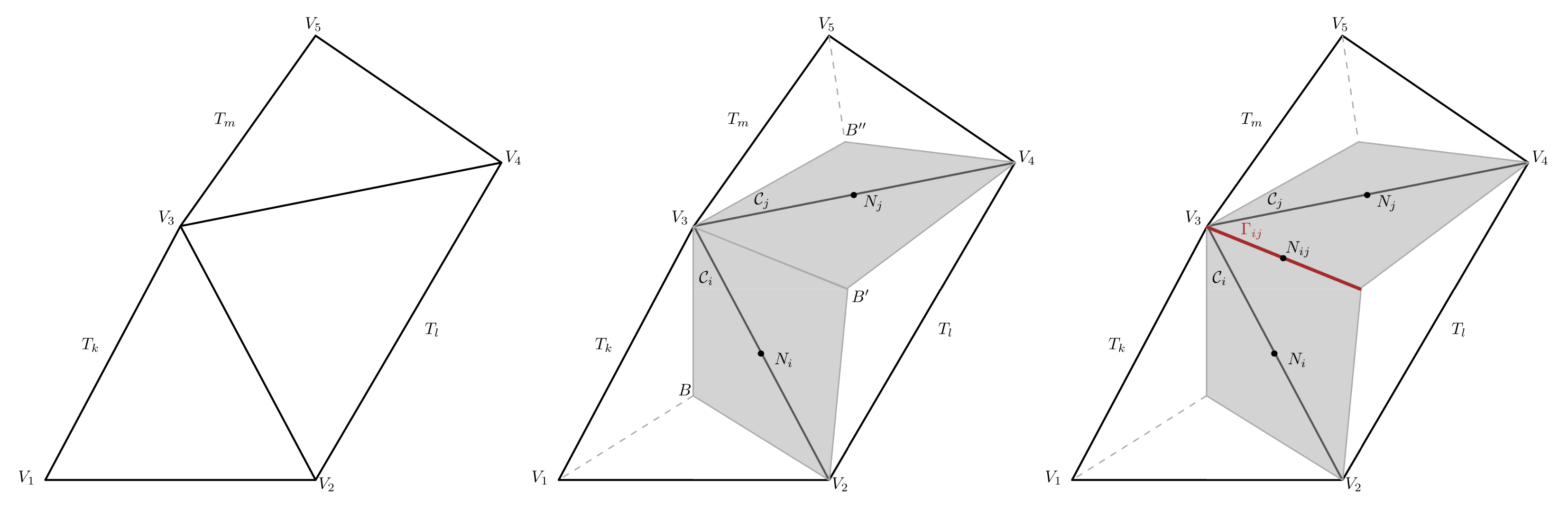
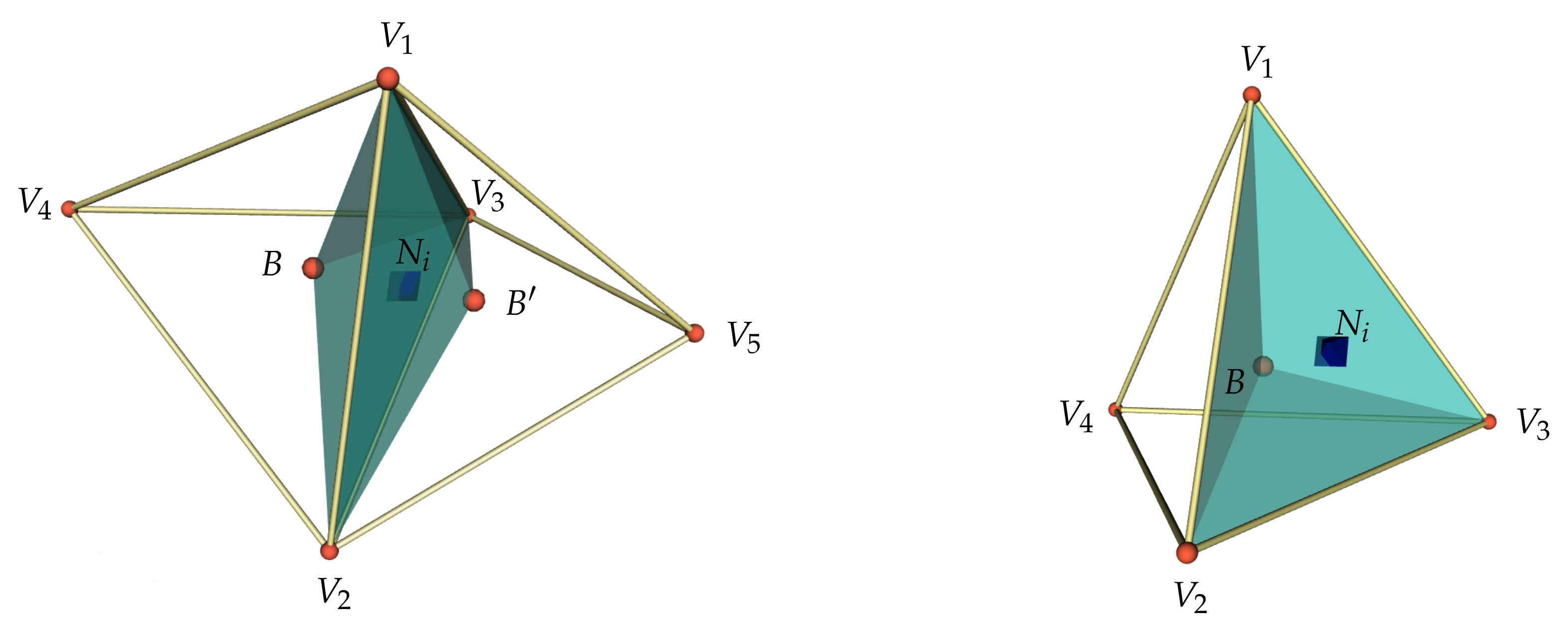
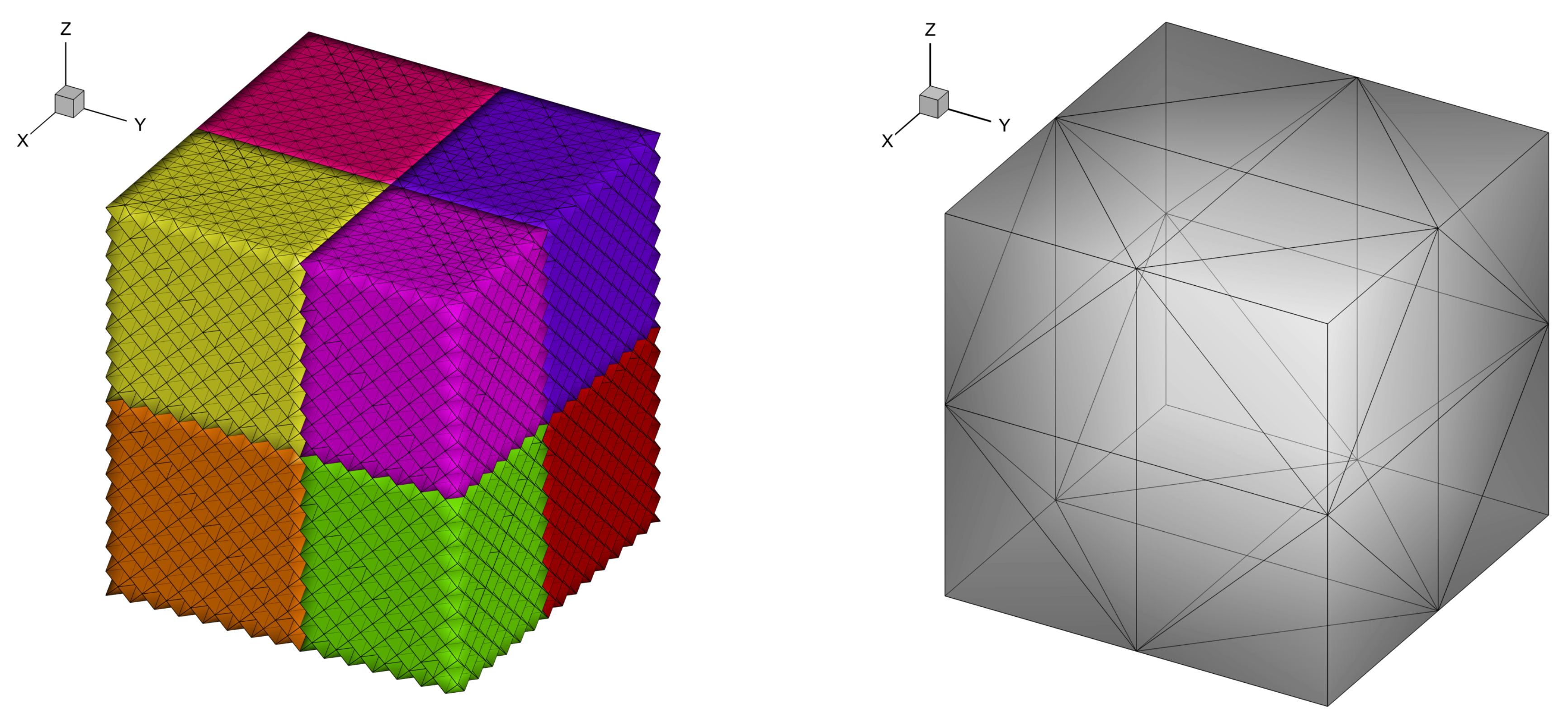
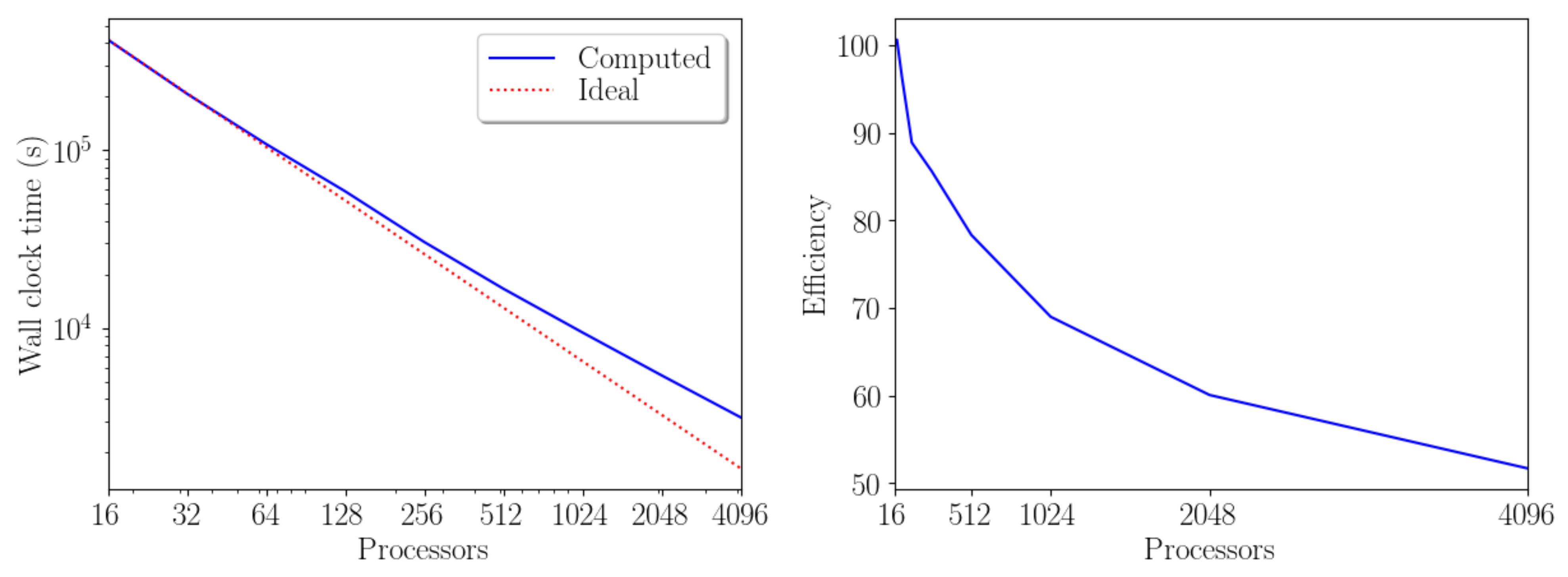
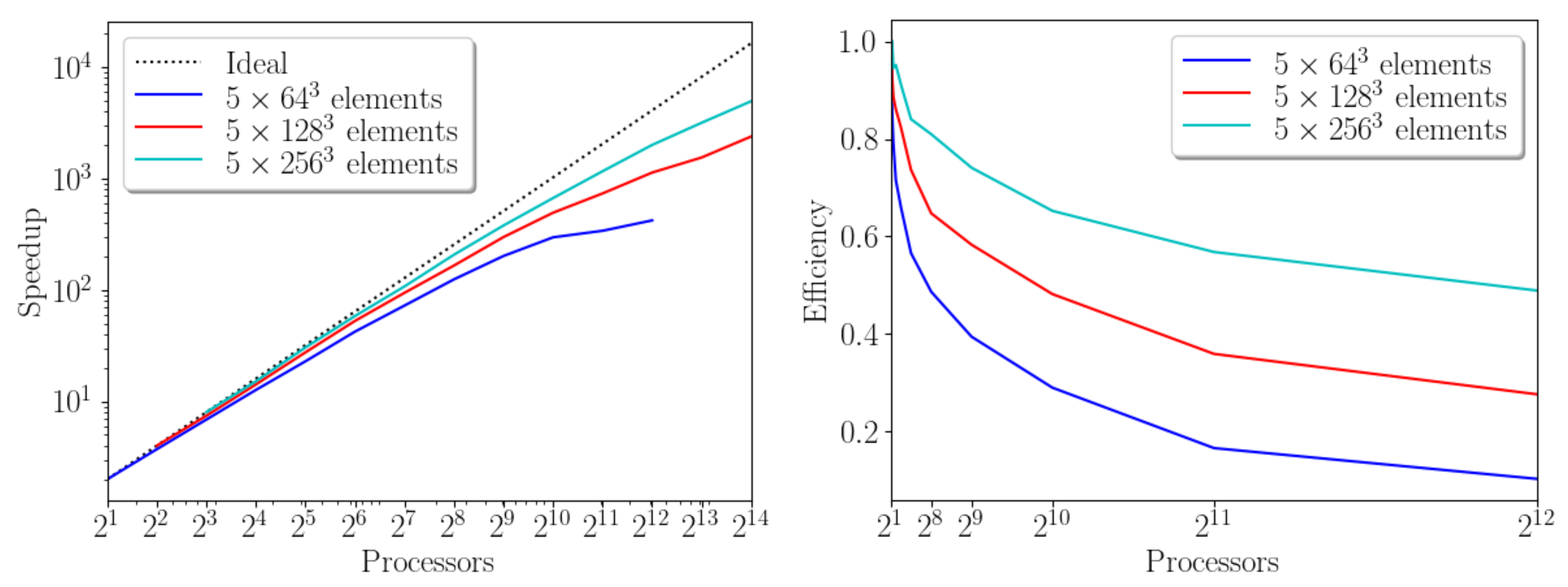
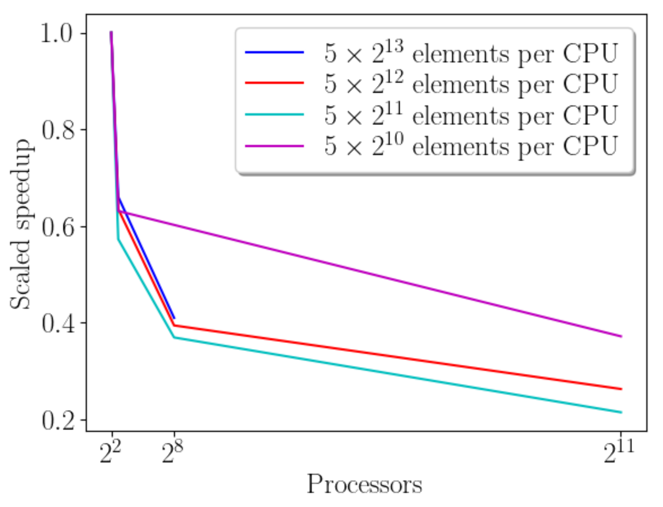
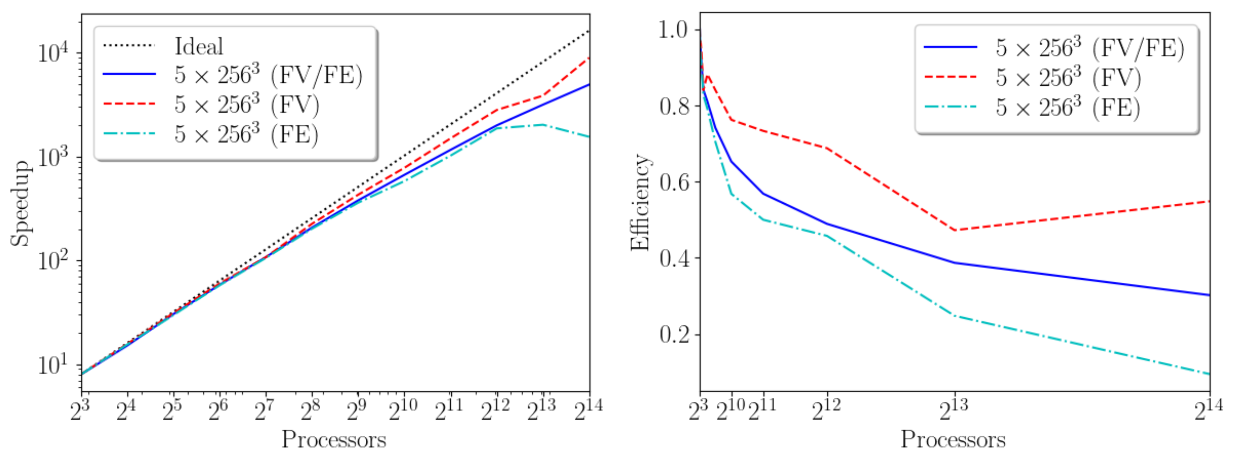
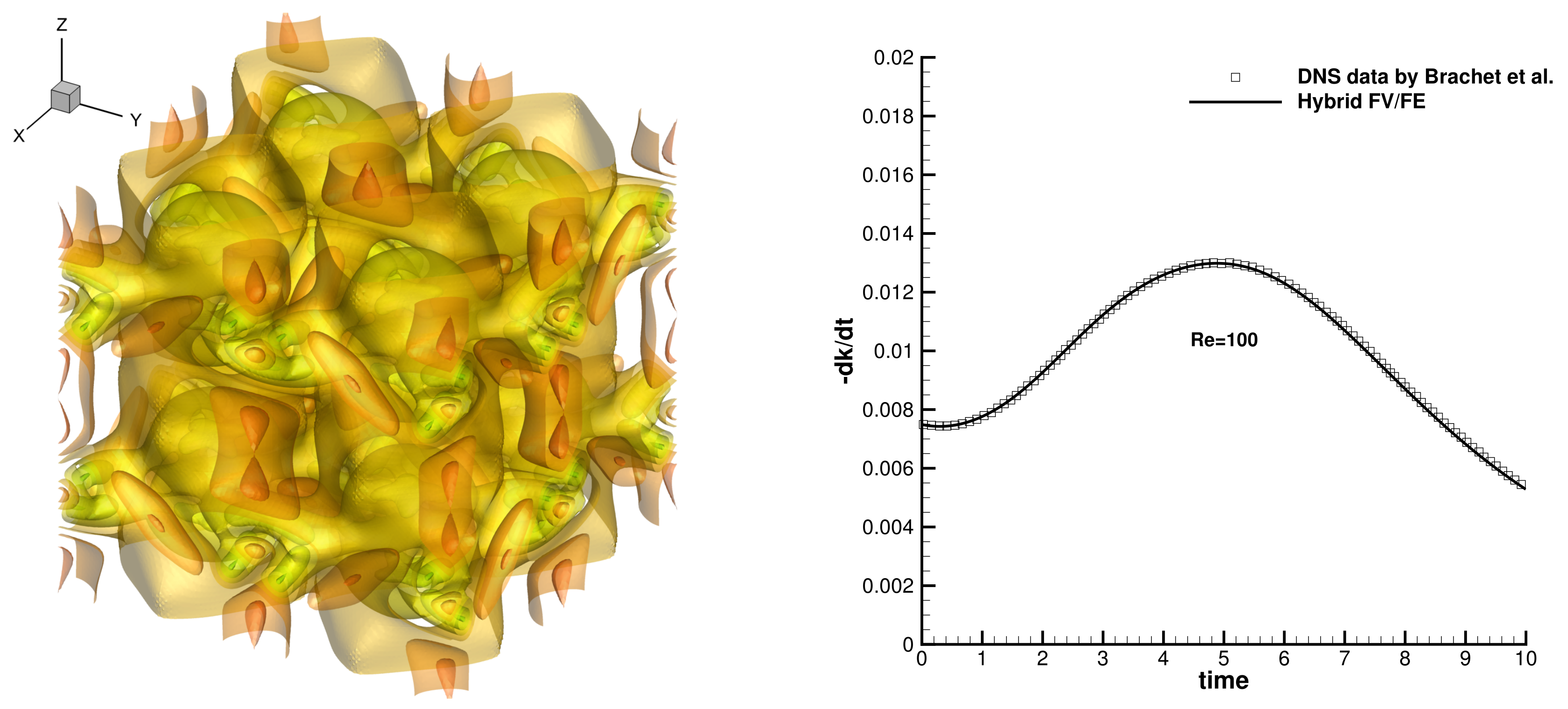
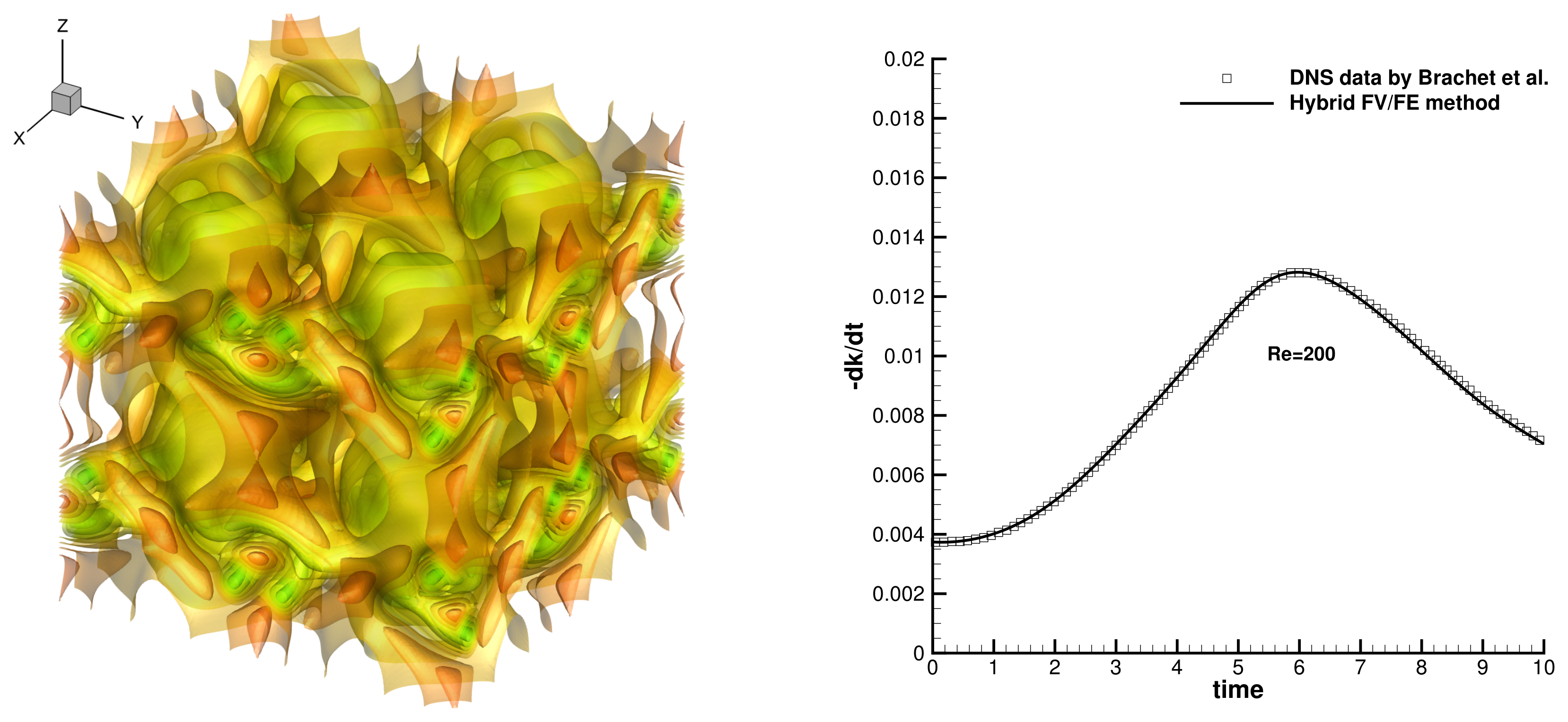
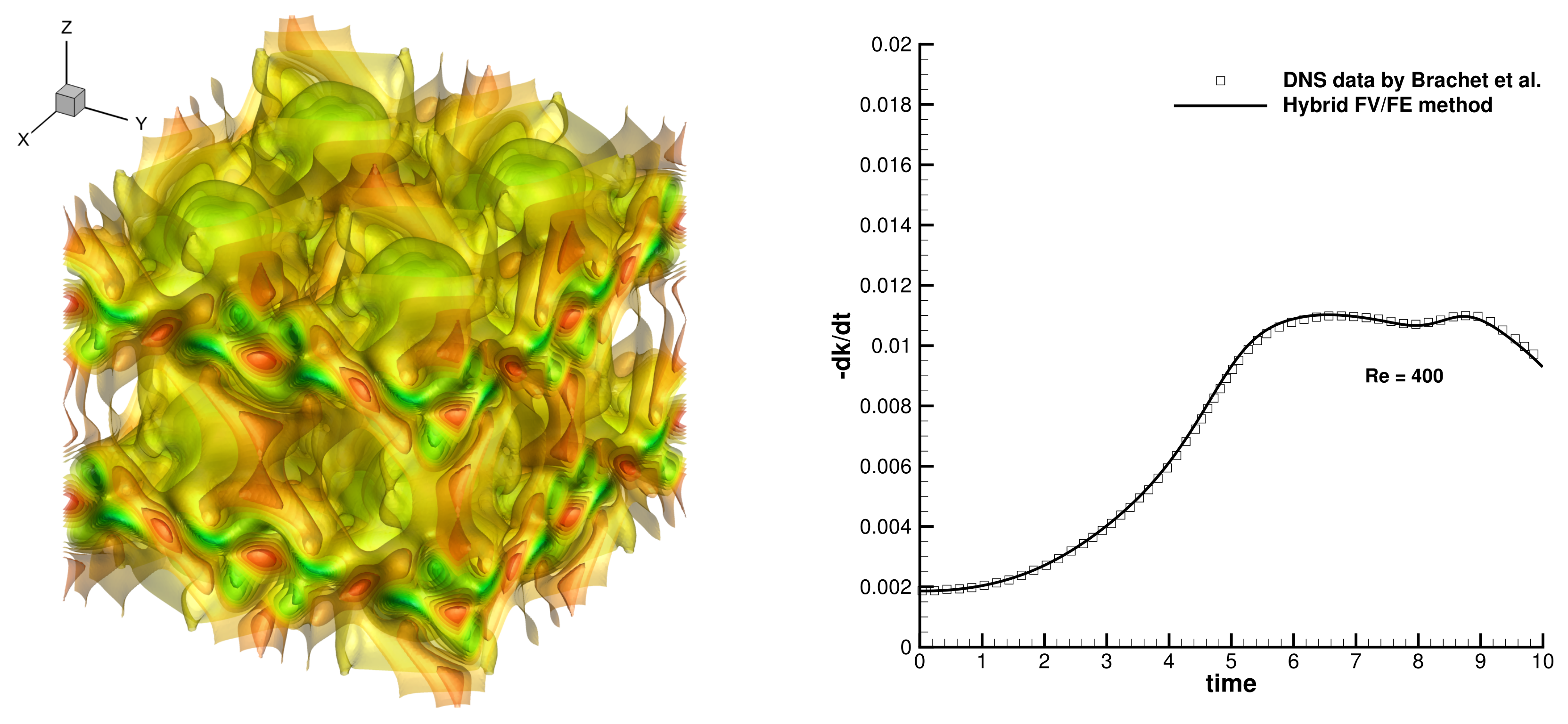
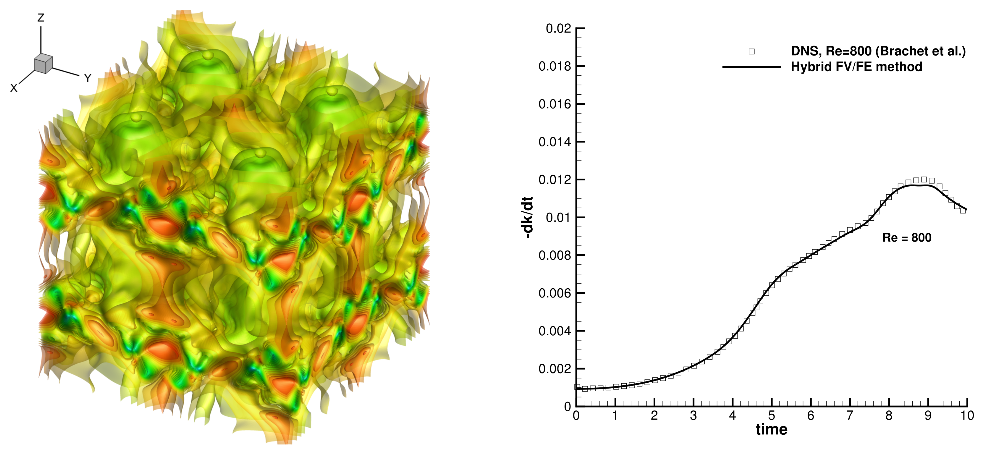
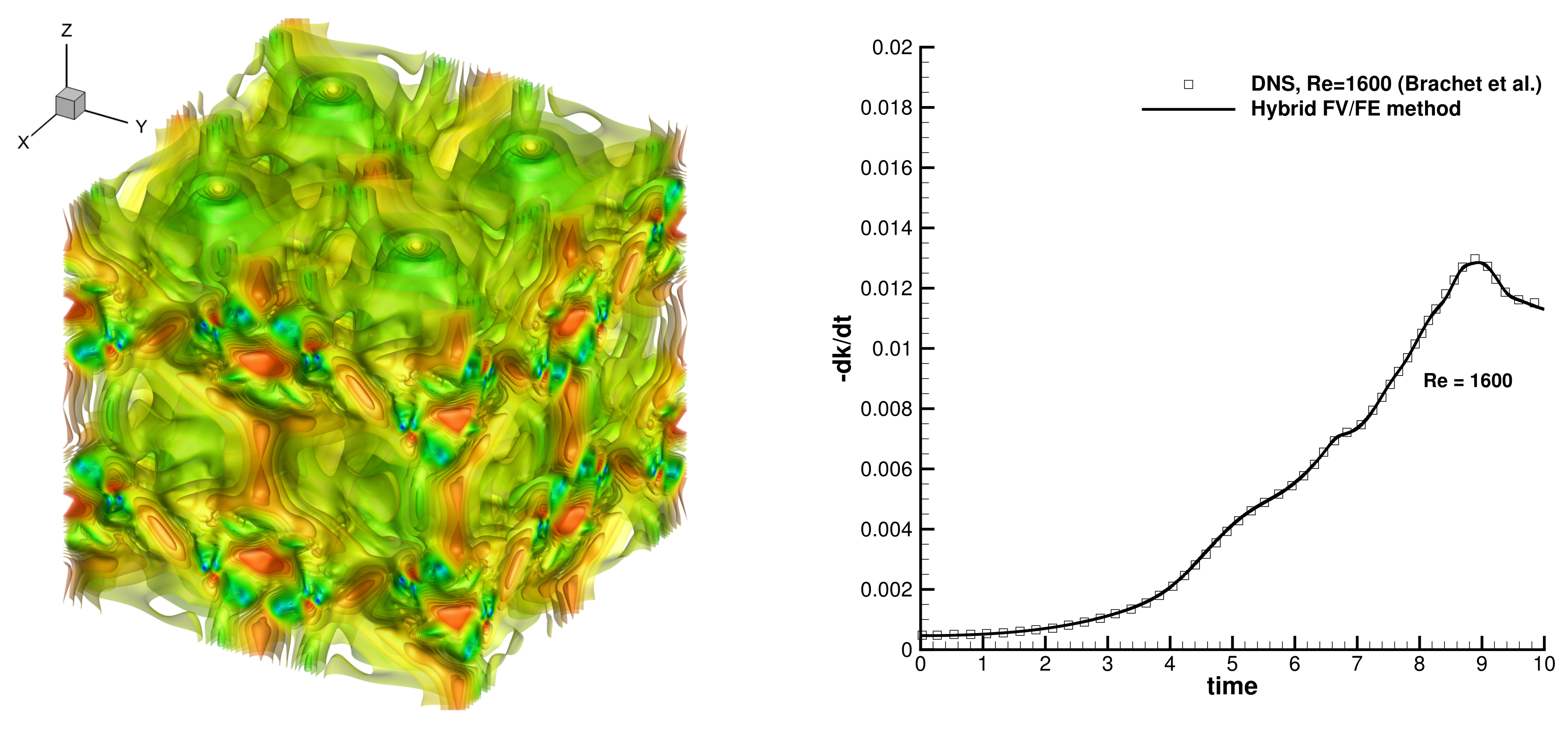
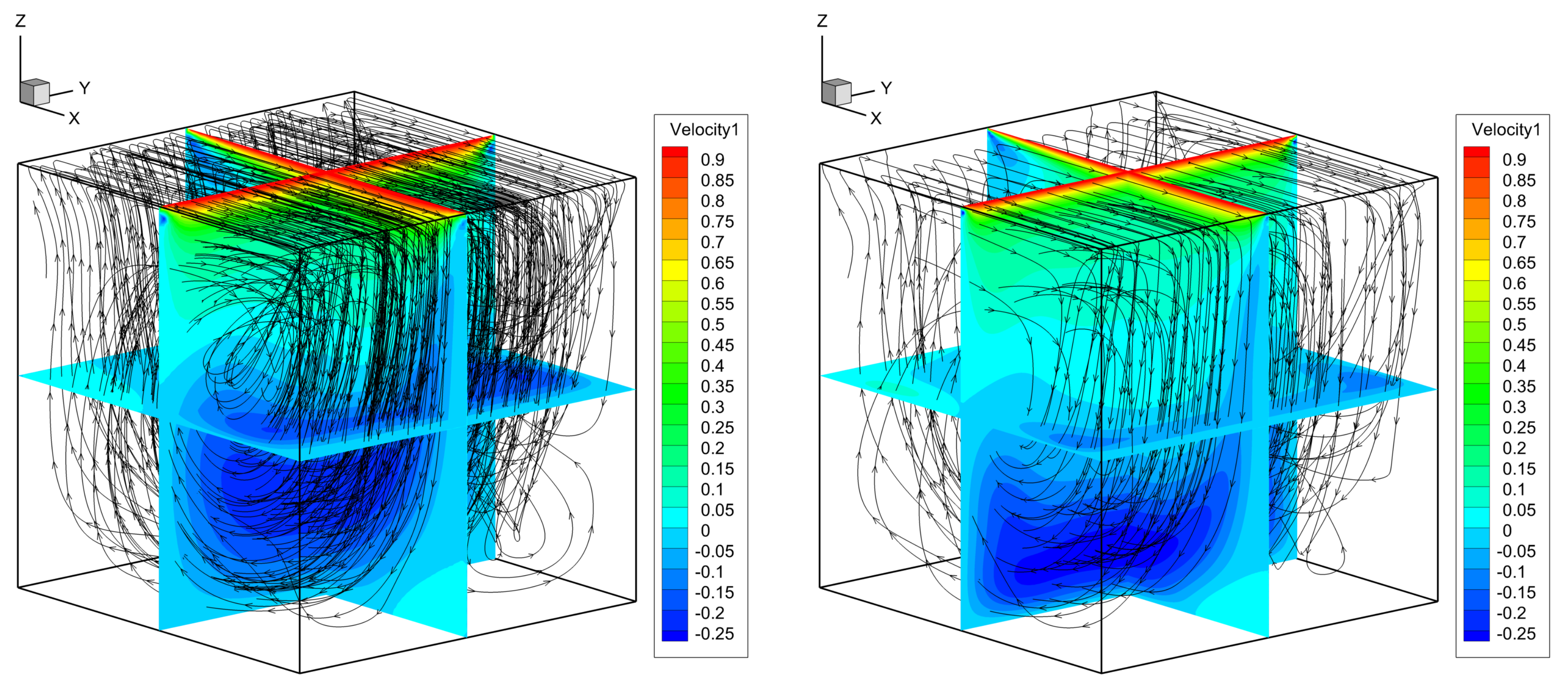
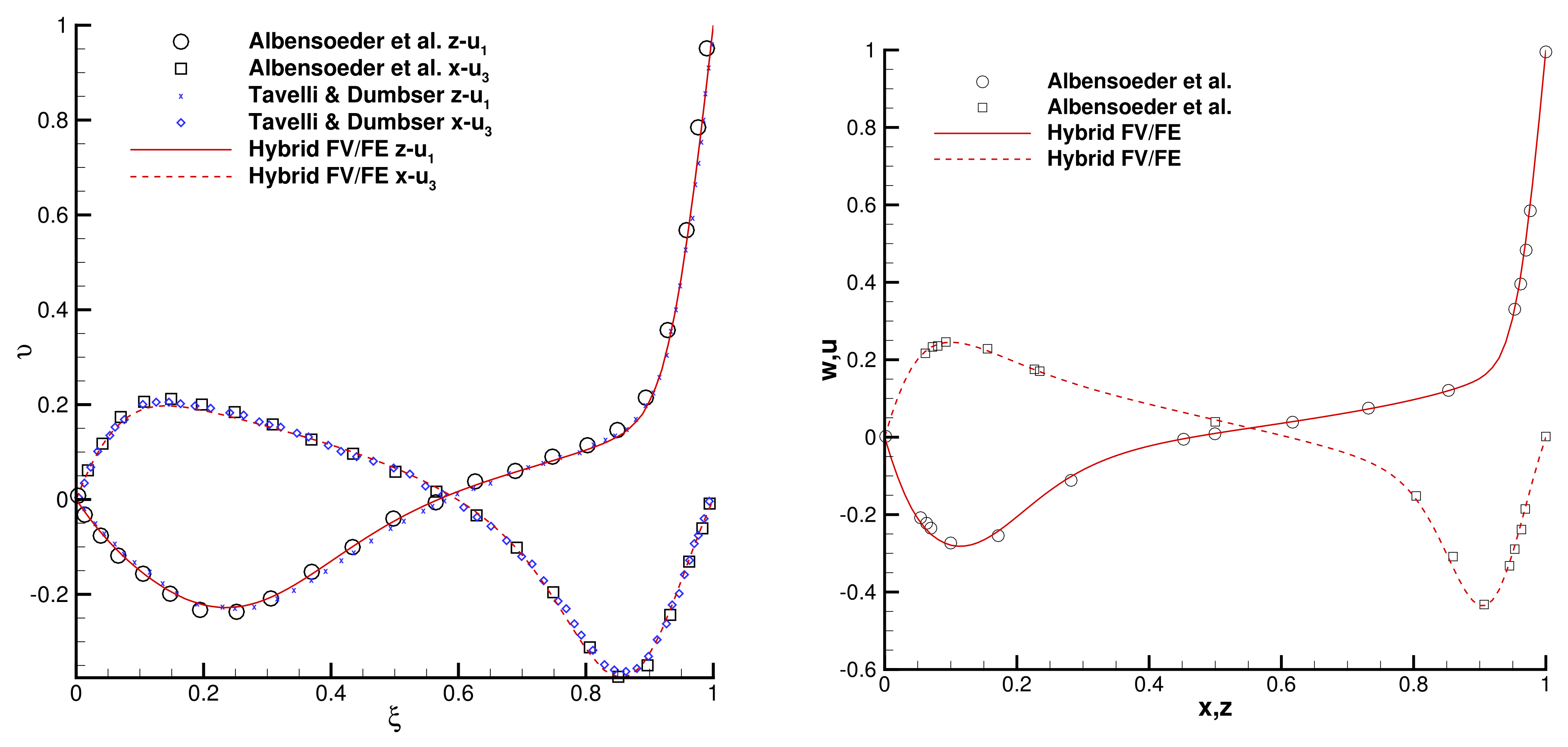
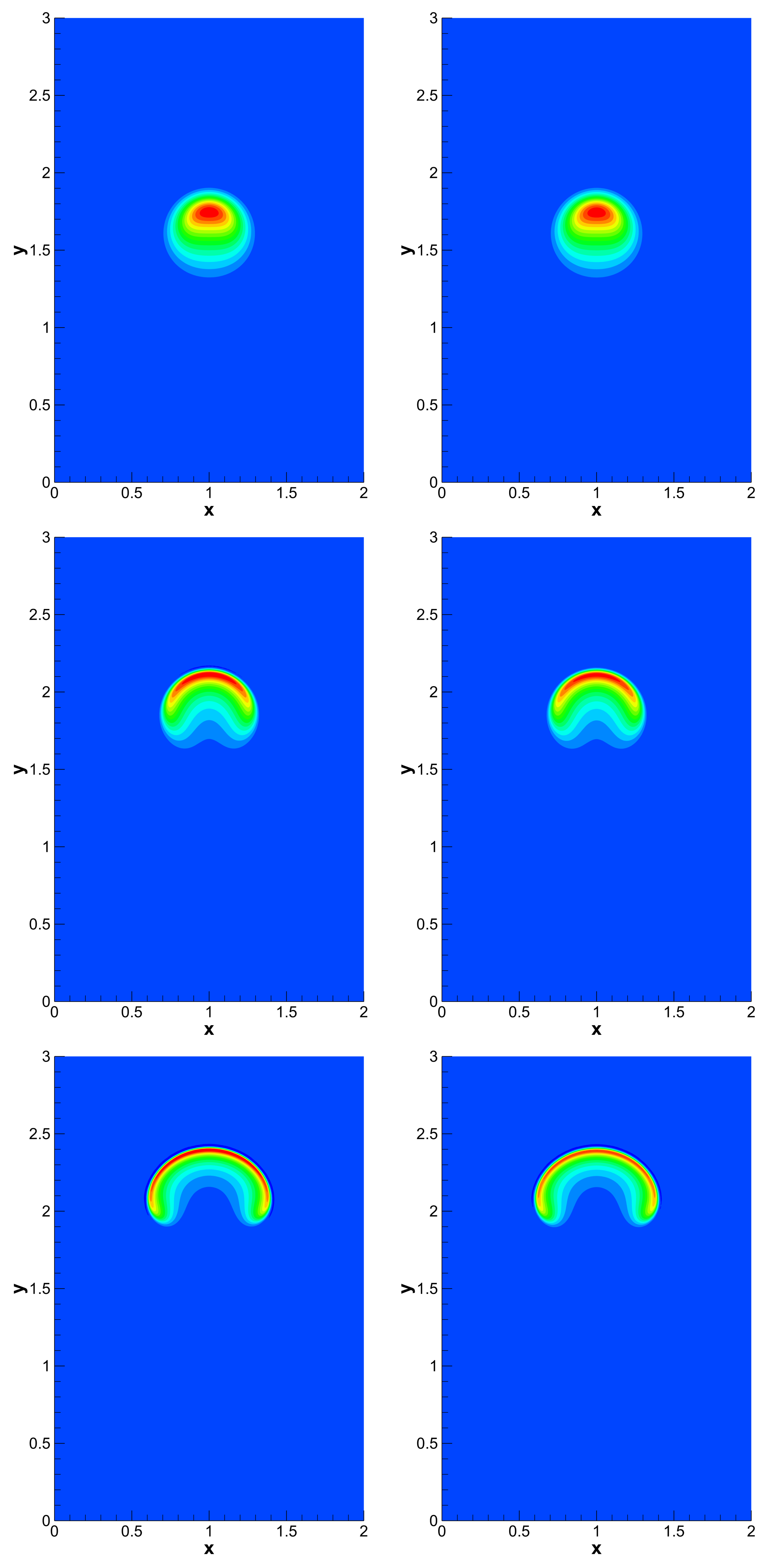
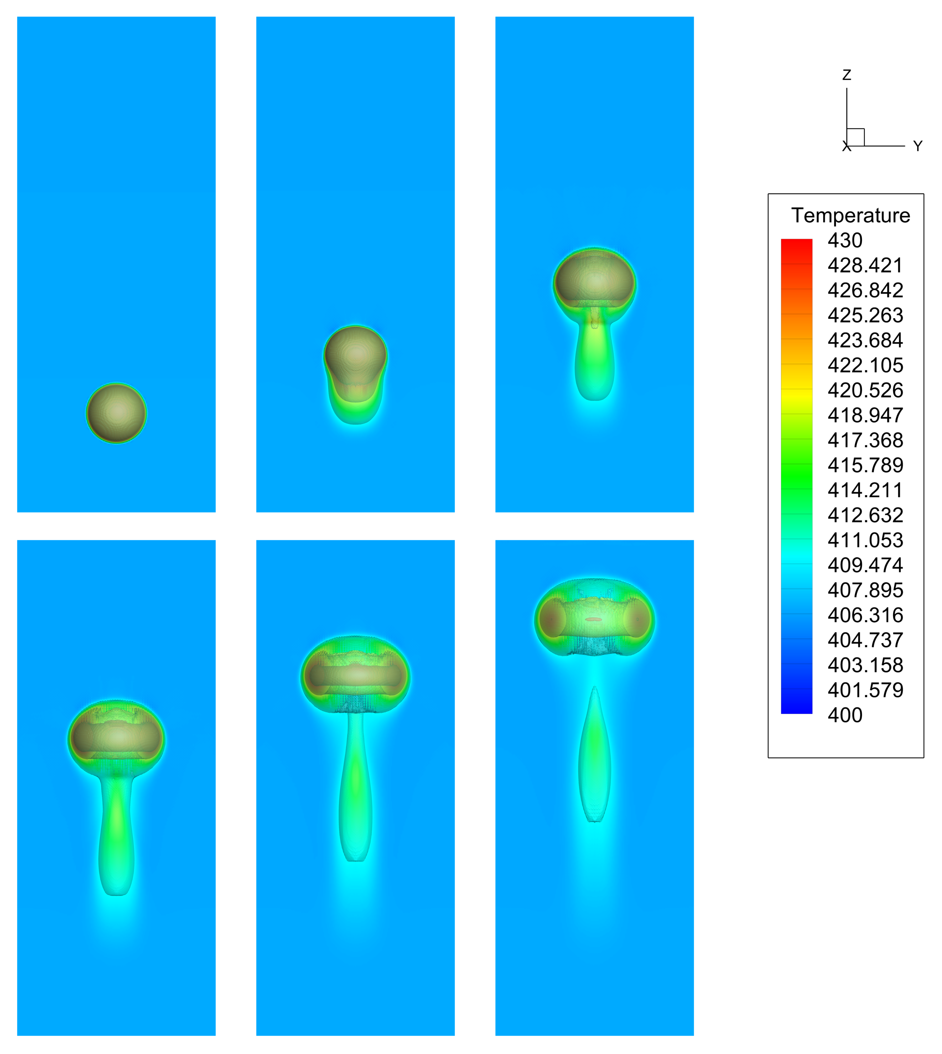
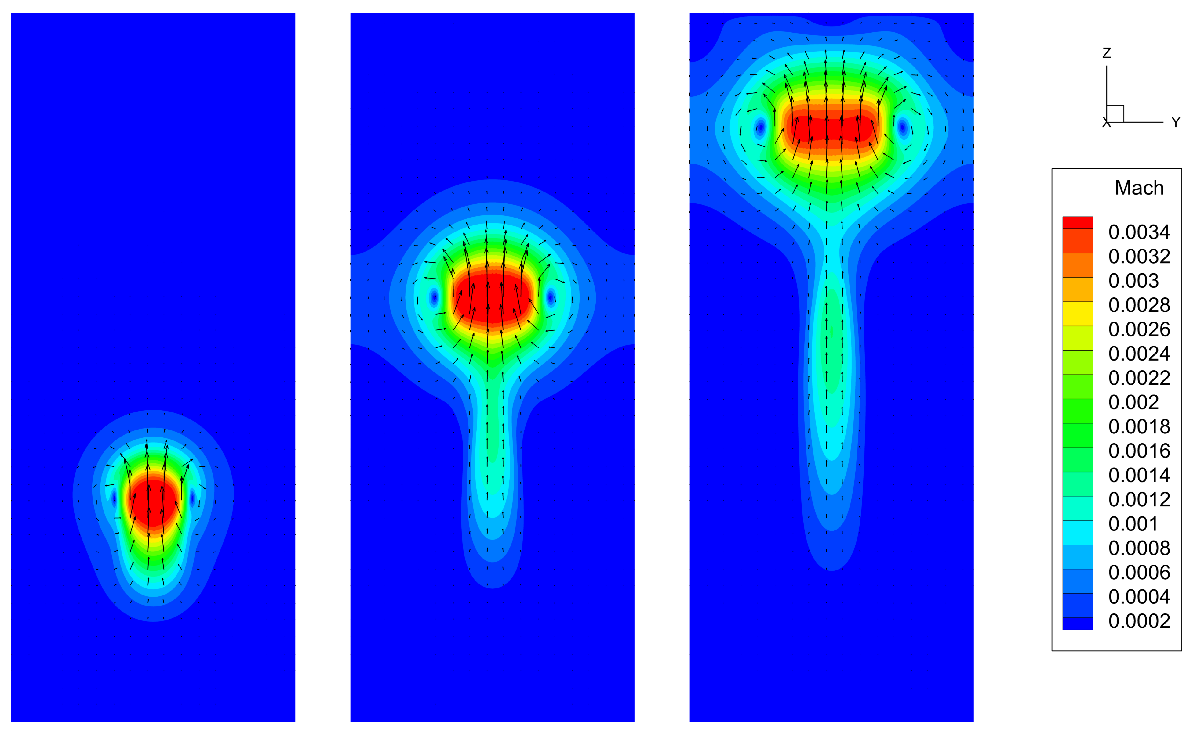
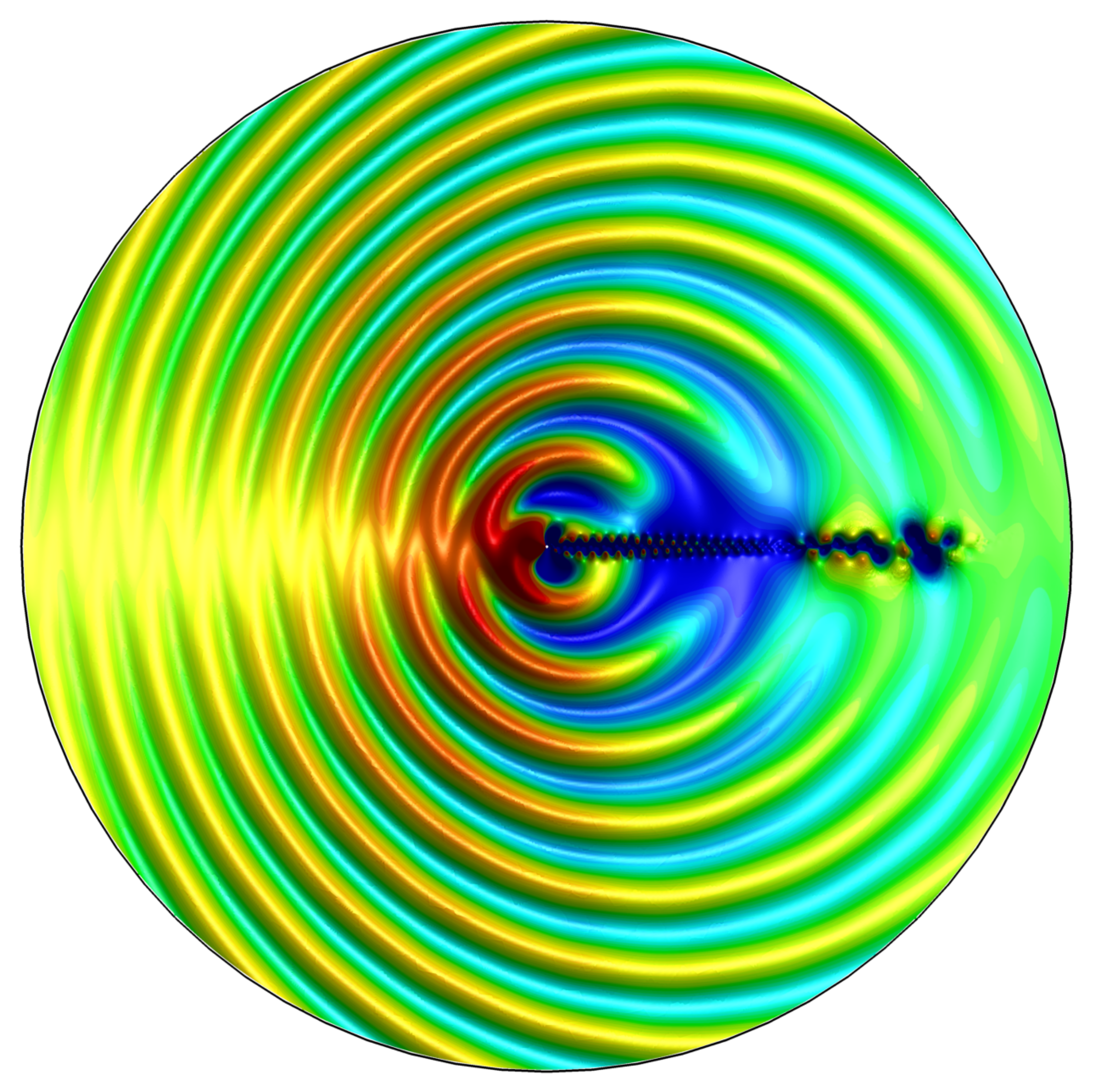
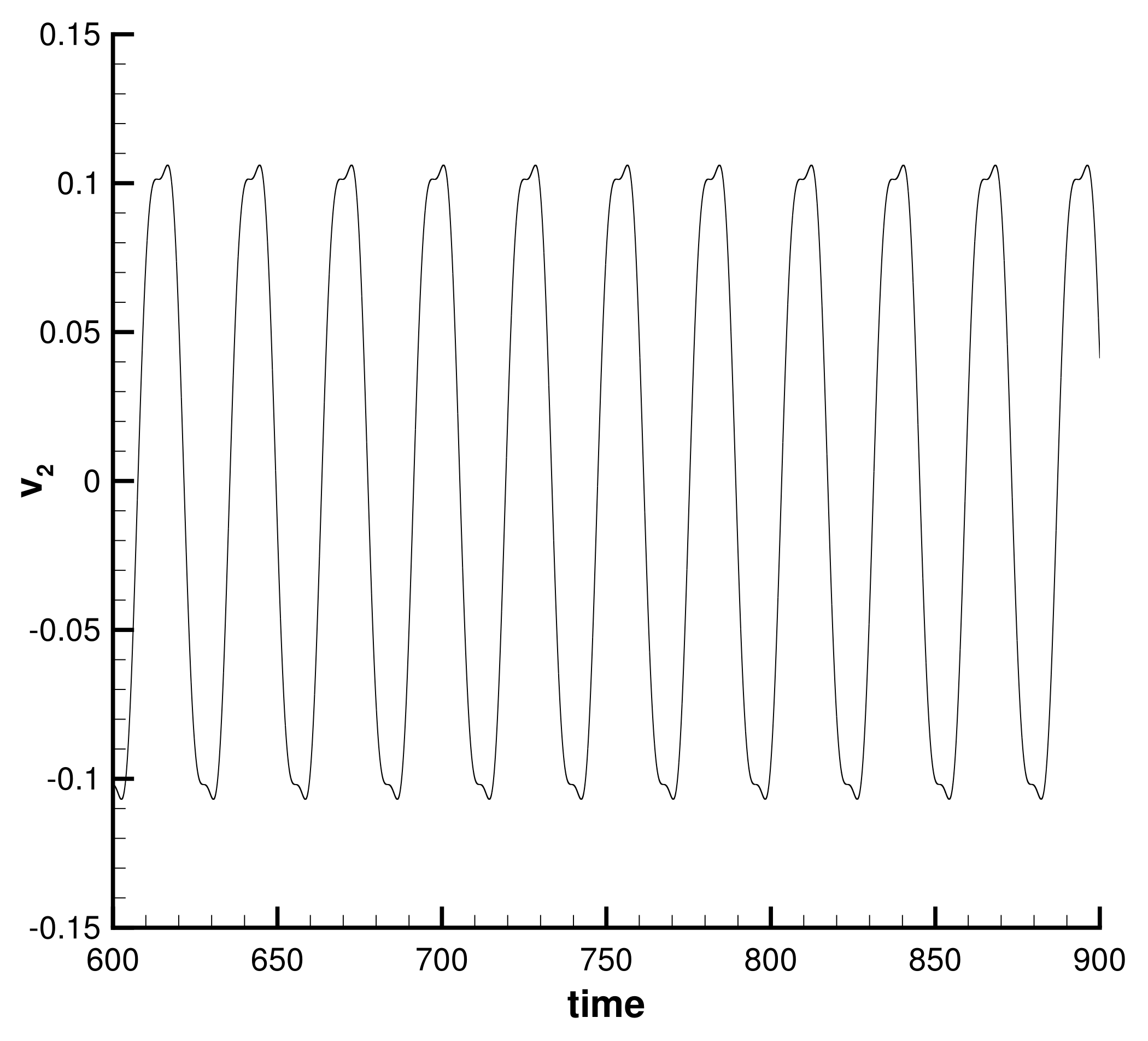
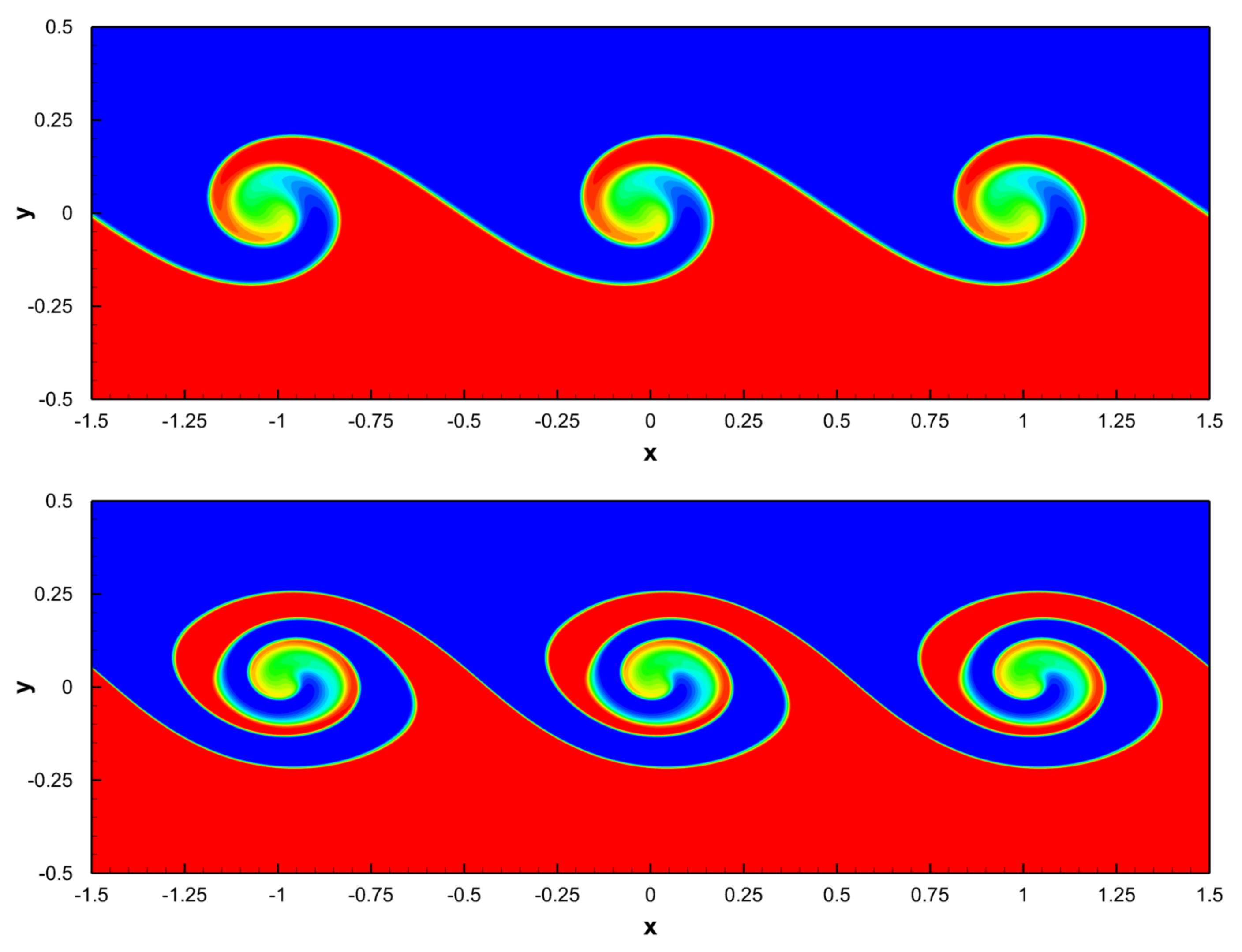
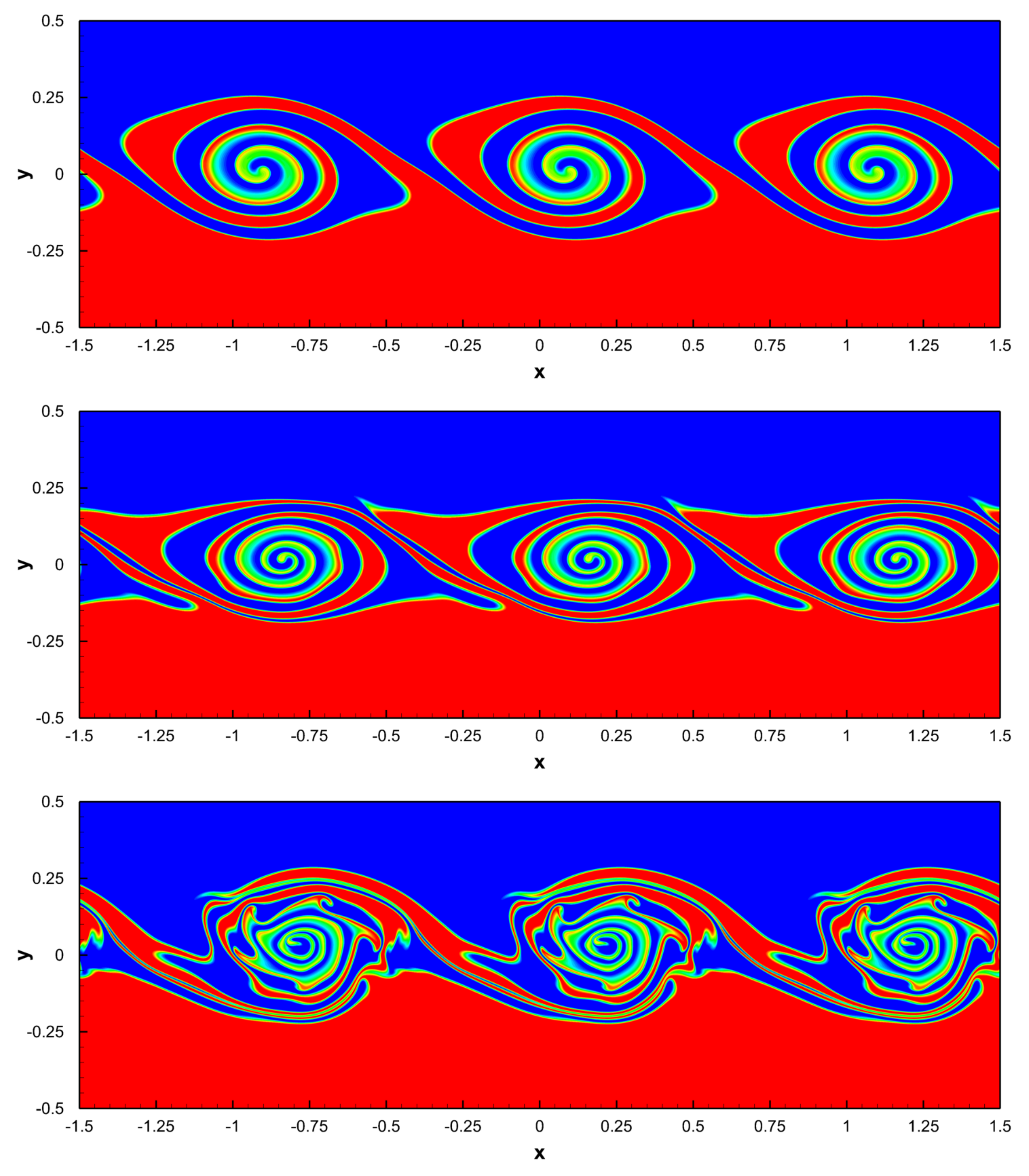
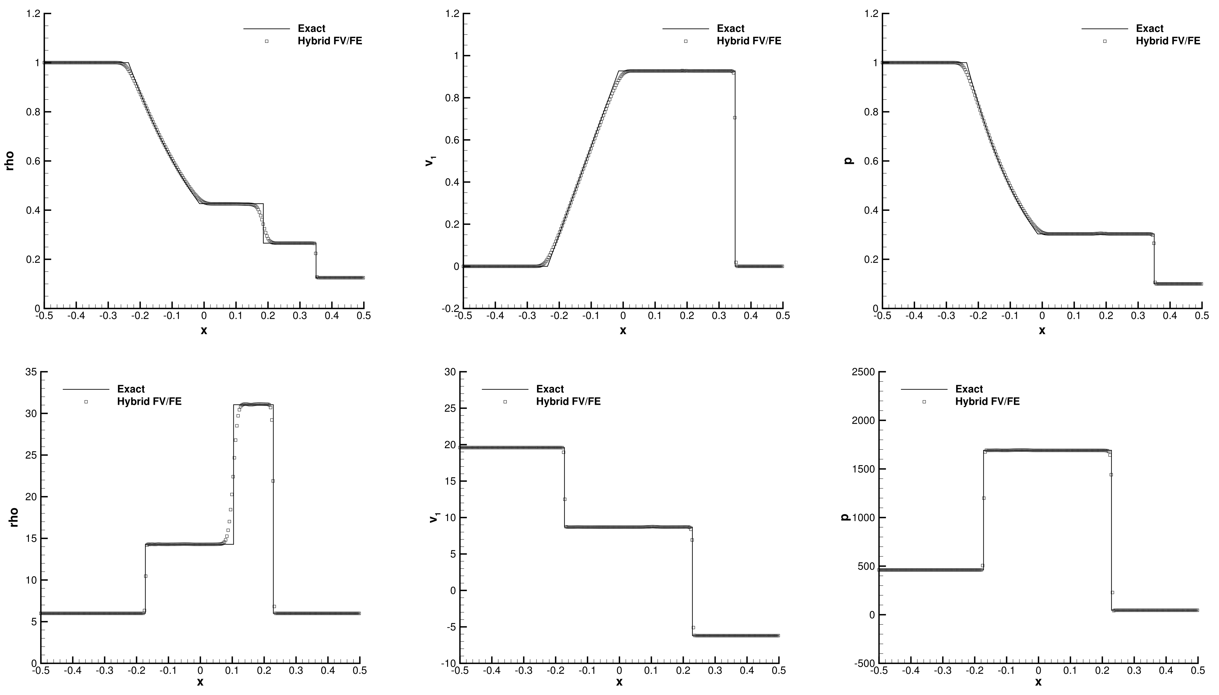
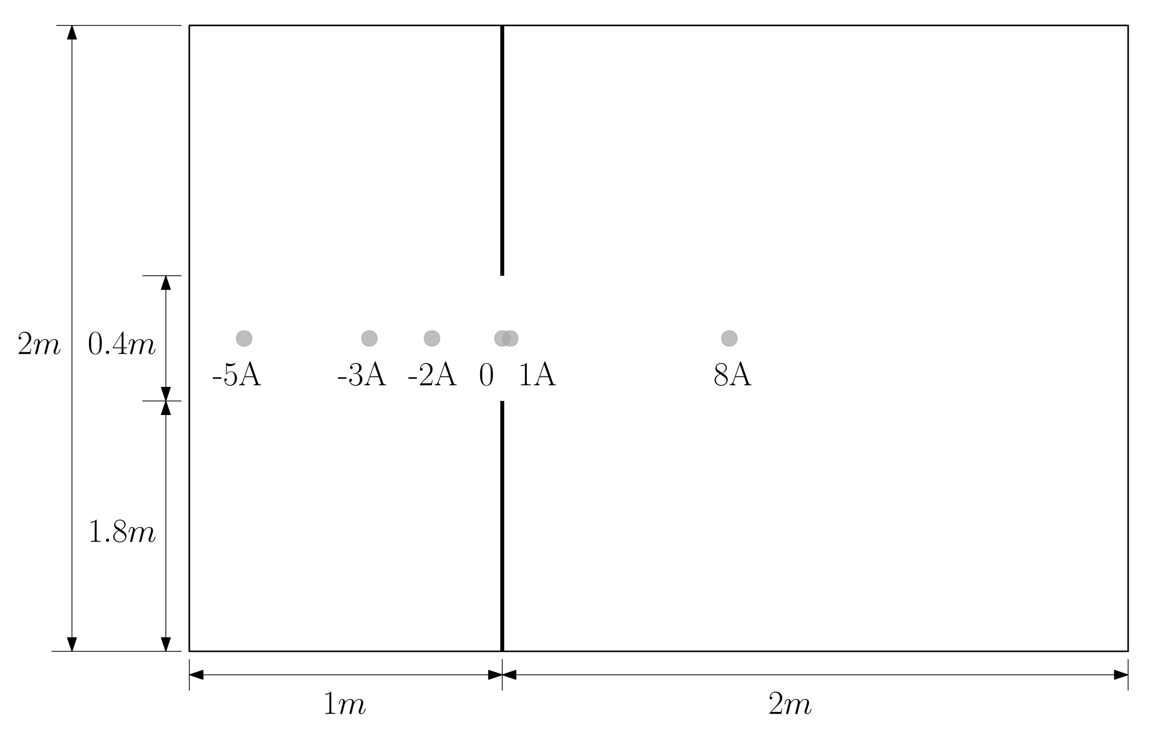
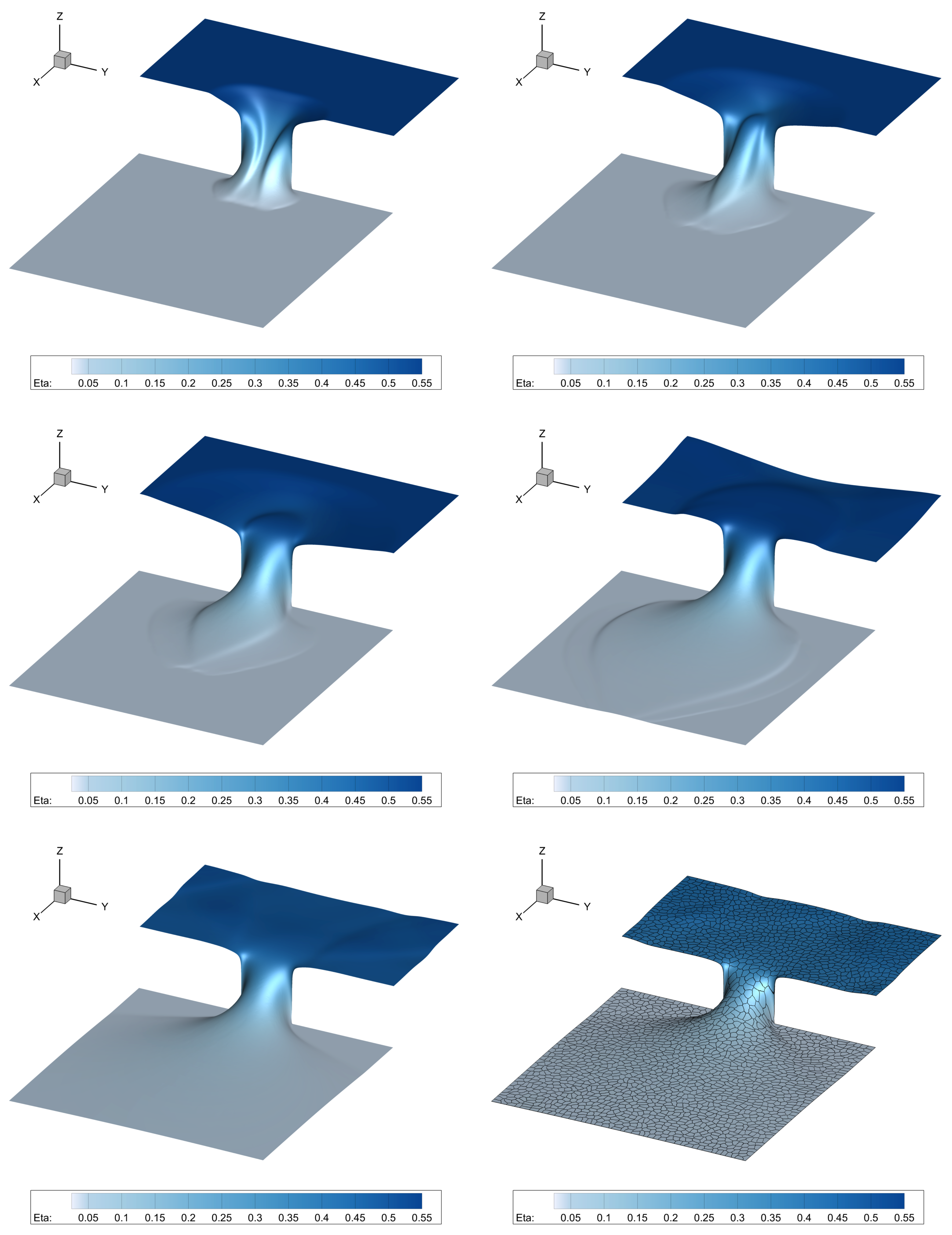
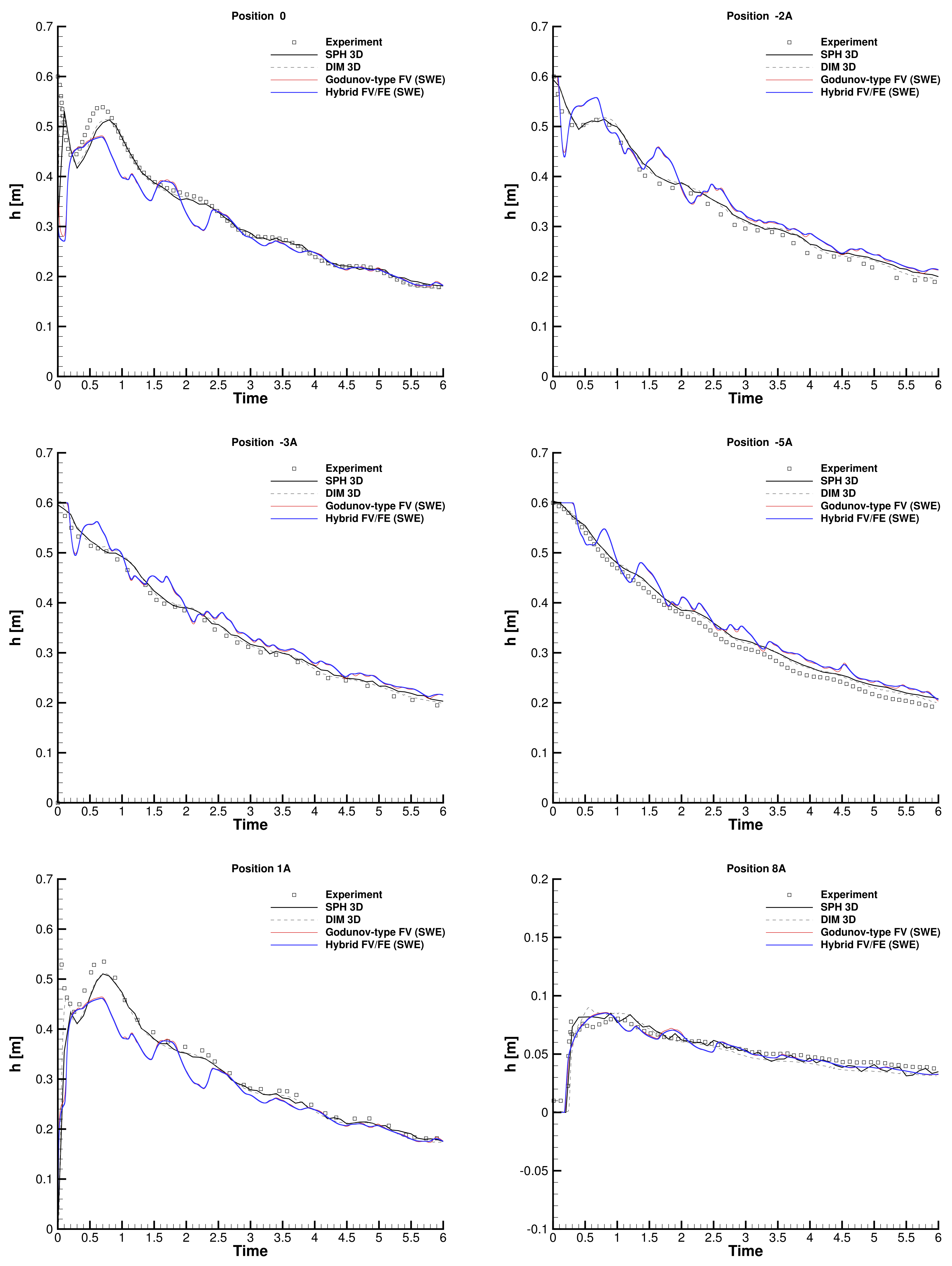
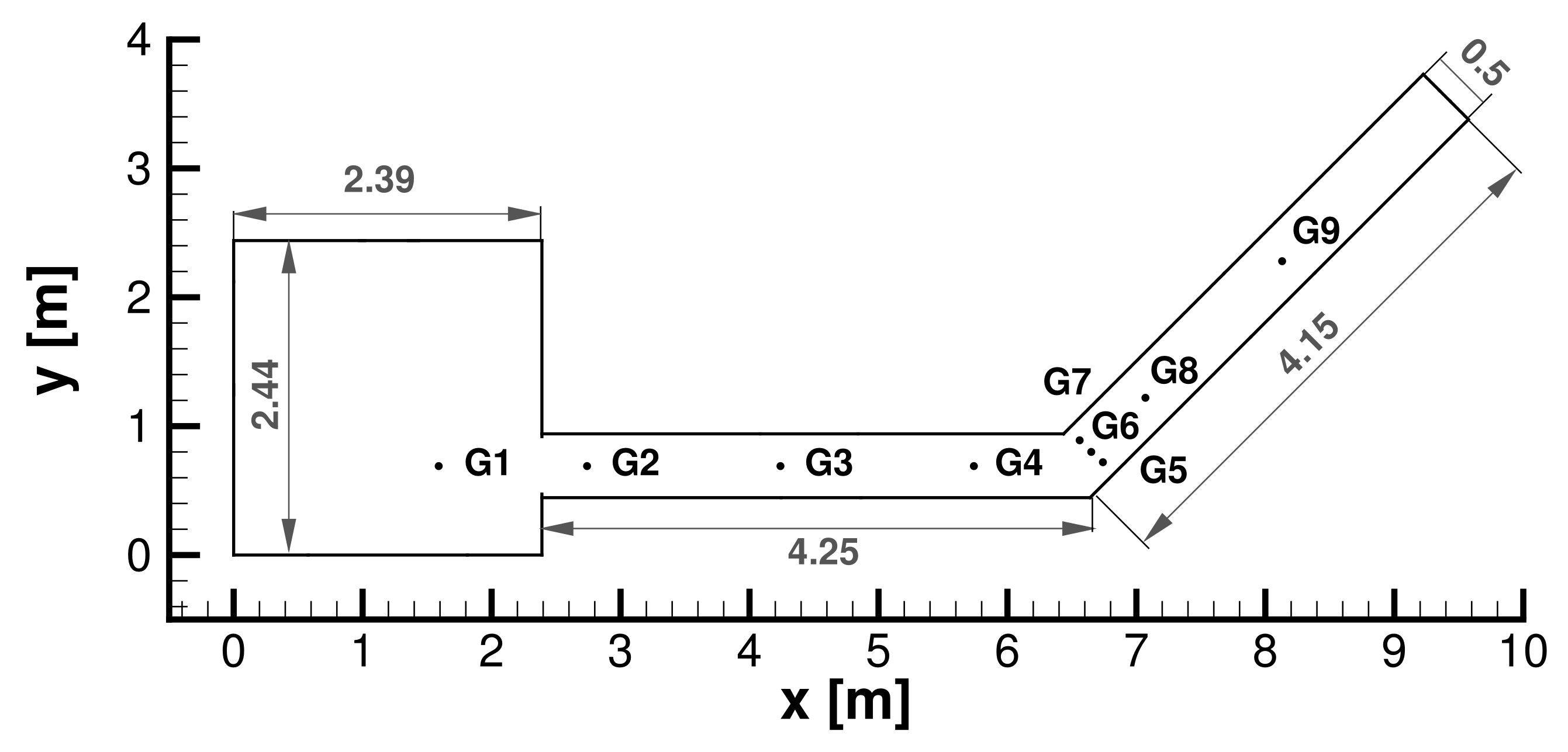
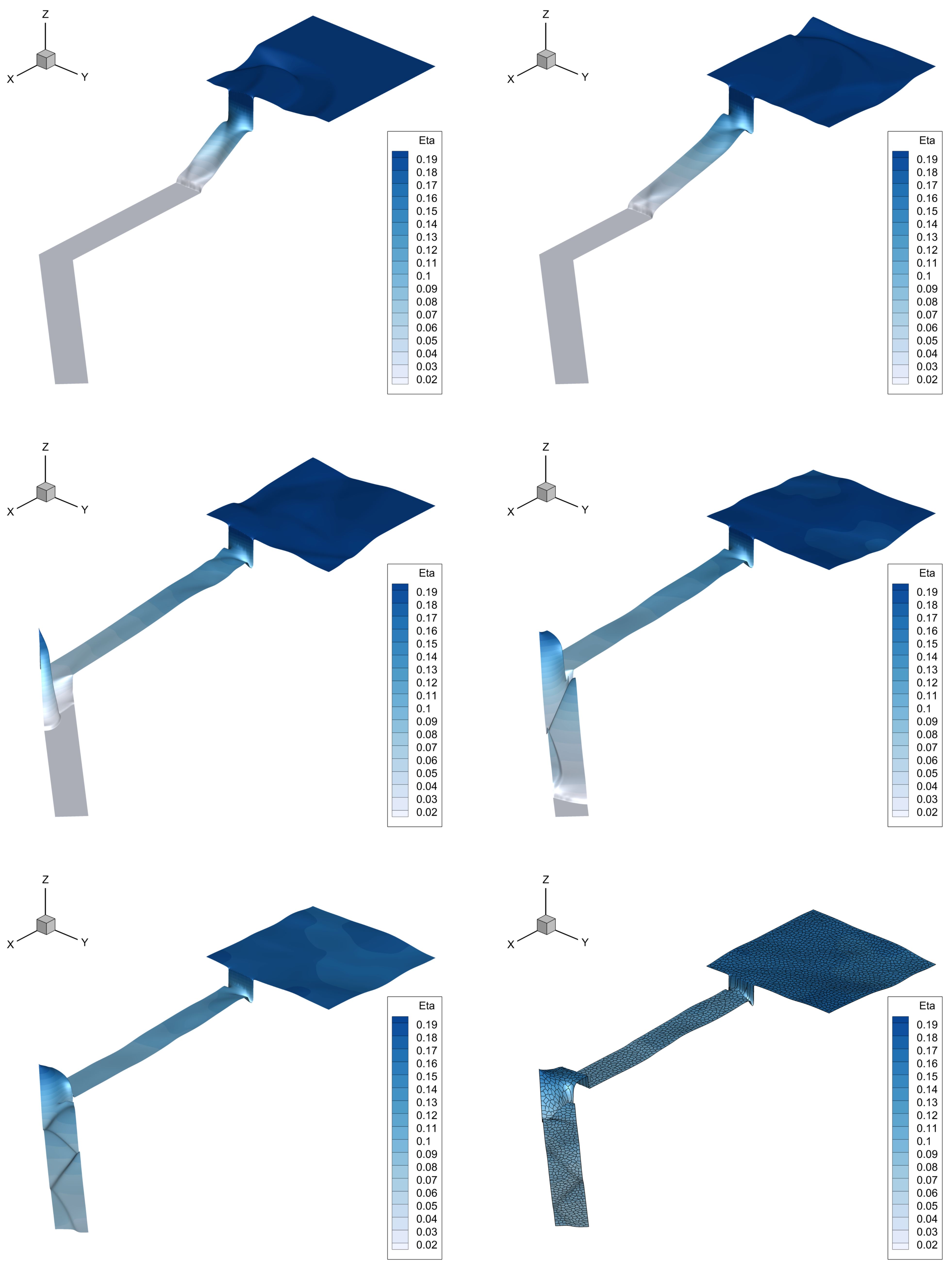
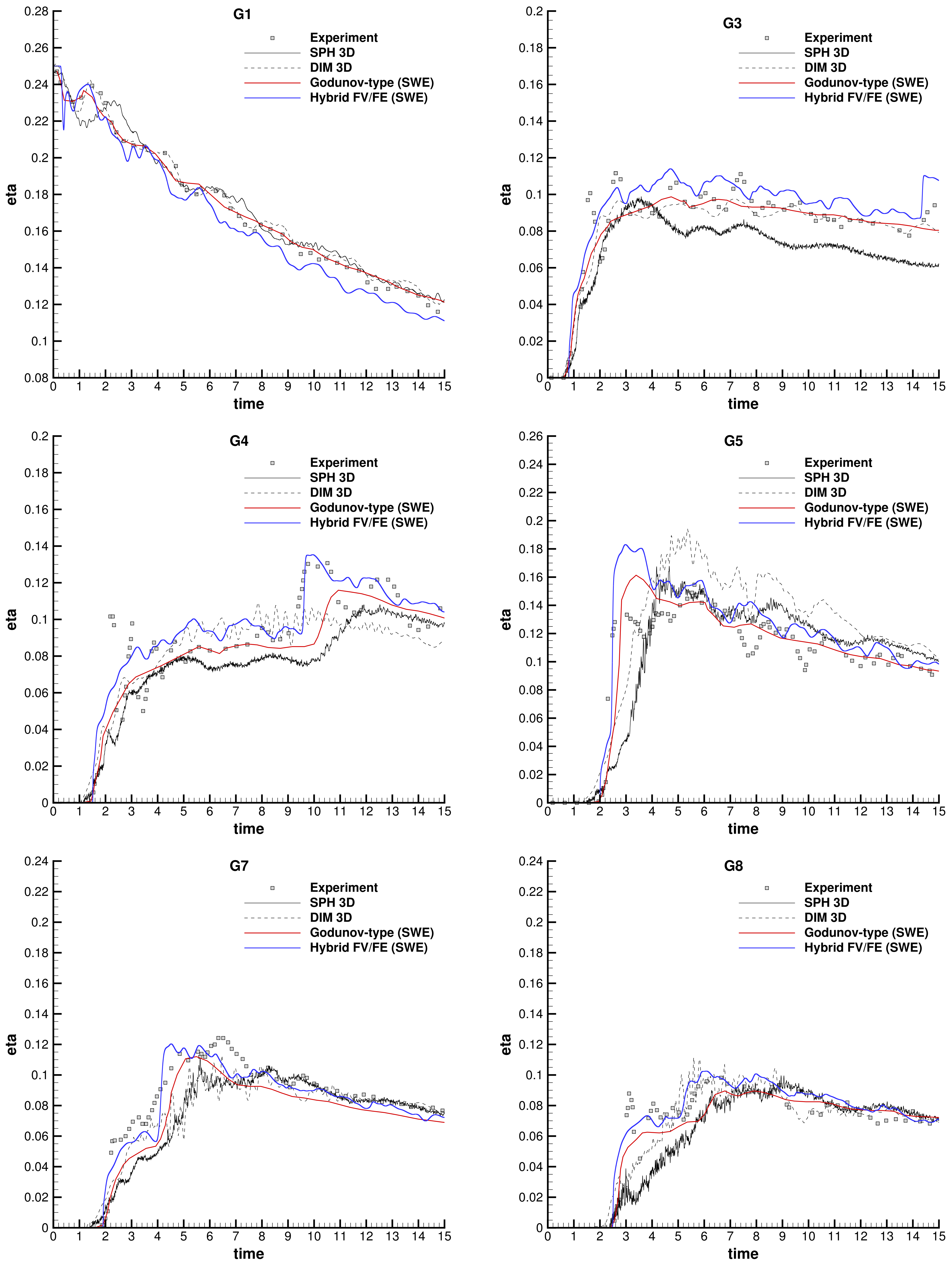
Table 1.
Description of the meshes and time steps used to perform the convergence analysis with the Taylor-Green vortex benchmark in 2D.
Table 1.
Description of the meshes and time steps used to perform the convergence analysis with the Taylor-Green vortex benchmark in 2D.
| Mesh | Elements | Vertices | Dual Elements | |
|---|---|---|---|---|
| 128 | 81 | 208 | ||
| 512 | 289 | 800 | ||
| 2048 | 1089 | 3136 | ||
| 8192 | 4225 | 12,416 | ||
| 32,768 | 16,641 | 49,408 | ||
| 131,072 | 66,049 | 197,120 | ||
| 524,288 | 263,169 | 787,456 | ||
| 2,097,152 | 1,050,625 | 3,147,776 | ||
| 8,388,608 | 4,198,401 | 12,587,008 |
Table 2.
Spatial error norms and convergence rates at time obtained using the LADER scheme for the Taylor-Green vortex benchmark in 2D.
Table 2.
Spatial error norms and convergence rates at time obtained using the LADER scheme for the Taylor-Green vortex benchmark in 2D.
| Mesh | ||||
|---|---|---|---|---|
| M1 | 4.13E−01 | 1.27E−01 | ||
| M2 | 1.16E−01 | 1.83 | 3.08E−02 | 2.04 |
| M3 | 2.99E−02 | 1.96 | 7.63E−03 | 2.01 |
| M4 | 7.54E−03 | 1.98 | 1.90E−03 | 2.00 |
| M5 | 1.89E−03 | 1.99 | 4.75E−04 | 2.00 |
| M6 | 4.74E−04 | 2.00 | 1.19E−04 | 2.00 |
| M7 | 1.19E−04 | 2.00 | 2.97E−05 | 2.00 |
| M8 | 2.97E−05 | 2.00 | 7.42E−06 | 2.00 |
| M9 | 7.42E−06 | 2.00 | 1.85E−06 | 2.00 |
Table 3.
Number of spatial divisions and number of MPI subdomains (CPU cores) along each coordinate direction of the grids used for the solution of the three-dimensional Taylor-Green vortex with different Reynolds numbers.
Table 3.
Number of spatial divisions and number of MPI subdomains (CPU cores) along each coordinate direction of the grids used for the solution of the three-dimensional Taylor-Green vortex with different Reynolds numbers.
| Re Number | ||
|---|---|---|
| 100 | 128 | 8 |
| 200 | 128 | 8 |
| 400 | 128 | 8 |
| 800 | 256 | 16 |
| 1600 | 512 | 32 |
Table 4.
Initial states left and right, initial position of the discontinuity , and final simulation time t for each Riemann problem.
Table 4.
Initial states left and right, initial position of the discontinuity , and final simulation time t for each Riemann problem.
| Test | t | |||||||
|---|---|---|---|---|---|---|---|---|
| RP1 | 1 | 0 | 0 | 1 | 0 | |||
| RP4 |
Table 5.
Coordinates of the wave gauges of the three-dimensional dambreak on a dry plane for a bi-dimensional domain .
Table 5.
Coordinates of the wave gauges of the three-dimensional dambreak on a dry plane for a bi-dimensional domain .
| Wave Gauge | −5 A | −3 A | −2 A | 0 | 1 A | 8 A |
|---|---|---|---|---|---|---|
| x | 0 | |||||
| y | 0 | 0 | 0 | 0 | 0 | 0 |
Table 6.
Coordinates of the gauges G1–G8 of the CADAM test case.
| Gauge | G1 | G3 | G4 | G5 | G6 | G7 | G8 |
|---|---|---|---|---|---|---|---|
| x | 1.59 | 4.24 | 5.74 | 6.74 | 6.65 | 6.56 | 7.07 |
| y | 0.69 | 0.69 | 0.69 | 0.72 | 0.80 | 0.89 | 1.22 |
Publisher’s Note: MDPI stays neutral with regard to jurisdictional claims in published maps and institutional affiliations. |
© 2021 by the authors. Licensee MDPI, Basel, Switzerland. This article is an open access article distributed under the terms and conditions of the Creative Commons Attribution (CC BY) license (https://creativecommons.org/licenses/by/4.0/).
Share and Cite
MDPI and ACS Style
Río-Martín, L.; Busto, S.; Dumbser, M. A Massively Parallel Hybrid Finite Volume/Finite Element Scheme for Computational Fluid Dynamics. Mathematics 2021, 9, 2316. https://0-doi-org.brum.beds.ac.uk/10.3390/math9182316
AMA Style
Río-Martín L, Busto S, Dumbser M. A Massively Parallel Hybrid Finite Volume/Finite Element Scheme for Computational Fluid Dynamics. Mathematics. 2021; 9(18):2316. https://0-doi-org.brum.beds.ac.uk/10.3390/math9182316
Chicago/Turabian StyleRío-Martín, Laura, Saray Busto, and Michael Dumbser. 2021. "A Massively Parallel Hybrid Finite Volume/Finite Element Scheme for Computational Fluid Dynamics" Mathematics 9, no. 18: 2316. https://0-doi-org.brum.beds.ac.uk/10.3390/math9182316
Note that from the first issue of 2016, this journal uses article numbers instead of page numbers. See further details here.