
Simulated Annealing with Mutation Strategy for the Share-a-Ride Problem with Flexible Compartments
by
 , , and
Vincent F. Yu
1,2 ,
,
Putu A. Y. Indrakarna
1 ,
,
Anak Agung Ngurah Perwira Redi
3 and
Shih-Wei Lin
4,5,6,* 1
Department of Industrial Management, National Taiwan University of Science and Technology, Taipei 106, Taiwan
2
Center for Cyber-Physical System Innovation, National Taiwan University of Science and Technology, Taipei 106, Taiwan
3
BINUS Graduate Program—Master of Industrial Engineering, Industrial Engineering Department, Bina Nusantara University, Jakarta 11480, Indonesia
4
Department of Information Management, Chang Gung University, Taoyuan 333, Taiwan
5
Department of Industrial and Management, Ming Chi University of Technology, New Taipei 243, Taiwan
6
Department of Neurology, Linkou Chang Gung Memorial Hospital, Taoyuan 333, Taiwan
*
Author to whom correspondence should be addressed.
Mathematics 2021, 9(18), 2320; https://0-doi-org.brum.beds.ac.uk/10.3390/math9182320
Submission received: 4 August 2021
/
Revised: 2 September 2021
/
Accepted: 16 September 2021
/
Published: 19 September 2021
(This article belongs to the Section Engineering Mathematics)
Abstract
:The Share-a-Ride Problem with Flexible Compartments (SARPFC) is an extension of the Share-a-Ride Problem (SARP) where both passenger and freight transport are serviced by a single taxi network. The aim of SARPFC is to increase profit by introducing flexible compartments into the SARP model. SARPFC allows taxis to adjust their compartment size within the lower and upper bounds while maintaining the same total capacity permitting them to service more parcels while simultaneously serving at most one passenger. The main contribution of this study is that we formulated a new mathematical model for the problem and proposed a new variant of the Simulated Annealing (SA) algorithm called Simulated Annealing with Mutation Strategy (SAMS) to solve SARPFC. The mutation strategy is an intensification approach to improve the solution based on slack time, which is activated in the later stage of the algorithm. The proposed SAMS was tested on SARP benchmark instances, and the result shows that it outperforms existing algorithms. Several computational studies have also been conducted on the SARPFC instances. The analysis of the effects of compartment size and the portion of package requests to the total profit showed that, on average, utilizing flexible compartments as in SARPFC brings in more profit than using a fixed-size compartment as in SARP.
1. Introduction
Transportation in urban areas is often categorized into people’s transportation and goods transportation. These two categories are most often treated separately due to their separate transportation needs. The recent trend in urban mobility is to consider more flexible transportation services that are low cost and convenient. In urban areas, traditional public transportation has shown its limitation to meet user’s demands, particularly for adapting to events that have an on-demand specific request, whereas private transportation services (e.g., taxi) are relatively more expensive. In this study, we considered combining the means of transporting people and goods in a transportation sharing mechanism, which offers potential benefits that induce flexible yet low-cost services. An example of this situation can be found in the ride-hailing taxi services, wherein, the taxi can deliver passengers and goods simultaneously during its services in a combined route.
The sharing mechanism of serving both people and goods provides more versatility and robustness of vehicle usage and taxi services. This concept was useful during the recent COVID-19 pandemic situation where people’s mobility is minimal. Despite the limitation of their mobility, the demand for goods and parcel delivery requests is increasing. In addition, a taxi service can utilize the flexibility of using the unused passenger seat as extra space for parcels to gain more capacity. This mechanism allows greater flexibility in routing and order assignment decisions. Thus, we propose a model that studies the scheduling of on-demand transportation to handle people and goods while considering also compartment sharing.
The models that consider on-demand people transportation are known as the dial-a-ride problem (DARP) [1], while the models that consider on-demand goods transportation are often categorized as variants of the pickup and delivery problem (PDP) [2]. The sharing mechanism of people and goods transportation was seldom investigated until Li et al. [3] proposed the share-a-ride problem (SARP). SARP considers schedules for several taxis to serve passenger transportation requests, and these taxis are permitted to transport parcels if this does not significantly affect the passengers’ riding time.
In 2016, two variants of the share-a-ride problem were introduced, one considered stochastic travel time, and the other considered stochastic delivery location [4]. Yu et al. [5] extended the SARP model to consider the hitchhiking situation where the passenger request is combined with a parcel request and another passenger request. The proposed model is denoted as the general share-a-ride problem (G-SARP). Beirigo et al. [6] introduced a mixed-purpose compartmentalized shared autonomous vehicle and parcel locker to the group of SARP problems and addressed it as the share a ride with parcel lockers problem (SARPLP). Likewise, Do et al. [7] considered a time-dependent model with speed windows where the speed of the vehicle is limited to a specific time and zone in the city. Their research used Tokyo’s transportation as the case study. Then, the cooperative SARP (coop-SARP) was presented by Cavagnini and Morandi [8], a SARP variant where a cooperation mechanism between transportation service providers is studied.
As one of the important future research directions, Yu et al. [5] suggested the consideration of capacity sharing between the passenger seat and luggage compartment. Multi-compartment is among many extensions of classical vehicle routing problems that have been studied extensively in recent years [9]. These variants are known as a multi-compartment vehicle routing problem (MCVRP). In MCVRP, the vehicles under use have multiple separate compartments that enable the collection of merchandise with different characteristics or joint delivery. Commonly, during transportation, different product types cannot be mixed in a single compartment. The application of MCVRP can be found in areas such as fuel distribution [10], waste collection [11], agricultural transportation [12,13], and maritime transportation [14,15].
From the perspective of problem complexity, both SARP and MCVRP are known to be NP-Hard [9,16]. Metaheuristic approaches are shown to be the popular choice to solve a problem with this type of complexity. Metaheuristics such as tabu search [17], adaptive large neighborhood search [16], simulated annealing [5,18], genetic algorithms [19], and ant colony optimization [20] have been shown to be capable of solving SARP, MCVRP, and its variants. Despite various applications of SARP and MCVRP, to the best of our knowledge, there is no literature that has previously considered the concept of shared compartments for the SARP.
This study presents the consideration of fully utilizing the capacity of a vehicle for running share-a-ride services. In the combined parcel and people transportation, the luggage compartment, also known as the trunk, is utilized to store the parcel, also named as a parcel compartment. The front and back seats are used for the passenger and are called the people compartment. In some situations, the number of parcel requests is more than the passenger requests. The model considered in this study allows the utilization of the people compartment to store a parcel, but not the reverse. The objective is to maximize the expected revenue generated from such a mechanism.
Following a literature survey, we found no previous study has addressed a model that considers shared compartments for SARP. Therefore, this study proposed a model that covers this situation and terms it share-a-ride problem with flexible compartments (SARPFC). Flexible compartments and slack times introduce a lot of infeasible solutions to the search space. To mitigate this problem, a modified simulated annealing heuristic was specially designed. A mutation strategy was employed to reduce search time and improve solution quality. The numerical experiments involve benchmark instances that have been presented earlier [5]. Our main contributions are as follows.
- We introduced a new variant of the share-a-ride problem—namely, the share-a-ride problem with flexible compartments (SARPFC).
- We formulated a mixed-integer linear programming (MILP) model for SARPFC.
- We propose a modified Simulated Annealing (SA) that includes a mutation strategy that is able to efficiently solve SARPFC.
- We performed comprehensive computational experiments with sensitivity analysis of the proposed algorithms and problem parameters.
In the remainder of this article, Section 2 presents the mathematical formulation of the share-a-ride problem with flexible compartments, Section 3 describes the details of the proposed algorithm, and Section 4 presents the numerical experiments conducted in this study. Finally, Section 5 presents the concluding remarks for this work.
2. Mathematical Formulation
SARPFC is defined on a complete undirected graph G = (V,A), where V is a vertex set partitioned into {Vp,Vf,{0, 2σ + 1}}. Vp and Vf correspond to the passenger and parcel request, respectively, while 0 and 2σ + 1 represent the origin and destination depot for a vehicle, respectively. More specifically, Vp = Vp,0 Vp,d, where Vp,0 represents the passenger origins and Vp,d is the passenger destinations. Similarly, Vf = Vf,0 Vf,d, where Vf,0 and Vf,d are the set of parcel origins and destinations, respectively.
Each vertex is associated with service time duration si ≥ 0 with s0 = s2σ+1 = 0 and time windows [,]. Each arc (i, j) ∈A is associated with travel distance dij and travel time tij. A set of taxis K is assumed to be ready in the depot at the beginning of the service. The aim is to maximize the total profit by finding a set of taxi routes that service all requests. Instead of using an identical fixed size compartment for each demand type c (n passengers and m parcels) such as in SARP, the proposed model introduces the flexibility of adjusting the compartment size based on several constraint limitations. The flexibility of adjusting the compartment is limited by a lower bound Bc and upper bound Ac for each demand type. Compartment capacity adjustment cannot exceed the original total capacity of the vehicle Zk. represents the conversion weight of each vehicle capacity for each demand type c to the sum of vehicle capacity. The maximum capacity of each compartment (c = 1 for passenger request and c = 2 for parcel request) can be adjusted not only for each vehicle or route but also for every visited node based on its demand .
A total number of requests ( = m + n) will be served by k number of vehicles, where each vehicle has a maximum work duration . For each time vehicle servicing a node, initial fare will be charged for a passenger and β initial fare for a parcel. For each km traveled by the vehicle, an additional fare is charged. The passenger will be charged fare per km and parcel delivery will be charged fare per km. It costs a vehicle per km to deliver any request. Each passenger request has its own maximum riding time . Because there is a possibility that a passenger ride is more than its direct riding time, a discount factor is used to calculate compensation for the passenger. A vehicle also can only service η number of requests between one passenger pickup and delivery. To track the number of requests in between, parameter is used to index the position of request i in a service sequence of the taxi. The formulations of SARPFC are defined as follows.
Decision variables:
- Binary decision variables are 1 if stop i and j served respectively by vehicle k.
- Arrival time for vehicle k at stop j.
- Load of vehicle k for demand type c upon leaving stop i.
- Ride duration of request i in vehicle k.
- Ratio between actual passengers riding time with their direct travel time.
- A maximum capacity of vehicle k for demand-type c at node i.
Objective function:
Constraints:
The objective function (1) is used to obtain the maximum total profit that consists of passenger fare, parcel fare, distance cost, and discount cost for a passenger’s extra riding time compared to direct driving. All requests are served exactly once by the same vehicle and enforced by constraint (2). The guarantee that each vehicle starts and ends its route at the depot is constrained by (3), (4), and (5). Constraint (6) ensures the same vehicle visit origin and destination nodes for a particular request. Except for the depot, every stop must have one preceding stop and one succeeding stop, which is defined in constraint (7). Constraint (8) defines the start of service times, constraint (9) defines vehicle loads, and constraint (10) defines riding times of passenger requests. Constraint (11) ensures that the total work duration for each vehicle must not exceed the vehicle operational time. Constraint (12) defines the time window constraints for the request. Constraint (13) defines the load of vehicle k after visiting vertex i, where it must not be larger than the maximum compartment capacity. Total capacity for all compartments must not exceed the total capacity for vehicle k as defined by constraint (14). Constraint (15) ensures that the capacity for each compartment lies between its upper and lower bounds. Constraint (16) ensures that the origin node will be visited before the destination node. The ratio between the actual riding time of a passenger and the corresponding direct travel time is ≥1 so that the last term in the objective function having a positive value is ensured by constraints (17) and (18). Constraint (19) determines that each passenger request has a duration when the service needs to be completed. Constraints (20) and (21) define the service sequence of the requests. The maximum inserted request between passenger pickup and drop-off point is defined by constraint (22). Constraint (23) shows the decision binary variable.
3. Solution Method
This study proposes a Simulated Annealing with Mutation Strategy (SAMS) algorithm for solving SARPFC. SA has been successfully used with similar problems, obtaining competitive results in various studies [5,21]. The following subsections describe the elements of the proposed SAMS.
3.1. Solution Representation
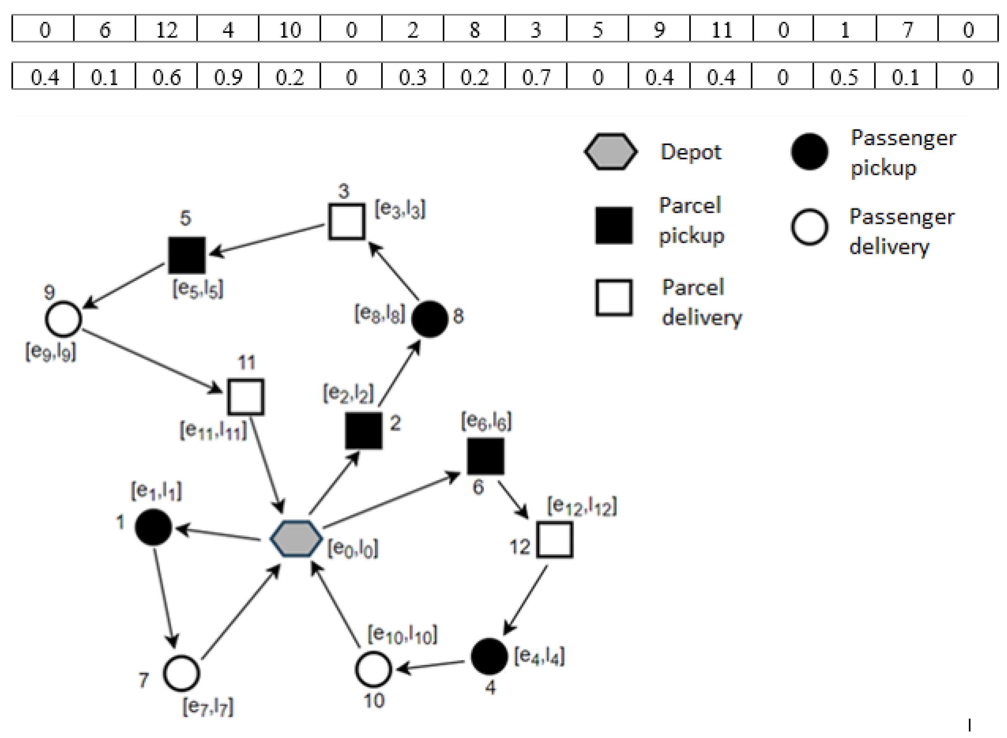
Two equal-length arrays are used as the solution representation for SARPFC. The first array comprises the depot node, n passenger pickup and delivery nodes, m parcel pickup and delivery nodes, and several dummy zeros as virtual depots. The number of dummy zeros is the same as the number of available vehicles. The first position and the last position must be a depot. Nodes are subsequently serviced one by one by a vehicle. If the following number in the representation is zero, then the route is ended, and the next vehicle will start a new route.
The second array consists of real numbers between 0 and 1, which are associated with the node in the first array. The second array is a ratio to determine how much slack time is assigned for each node from the maximum available slack time. Details regarding maximum slack time are explained by Yu et al. [5]. Figure 1 illustrates the solution representation for SARPFC.
3.2. The Initial Solution
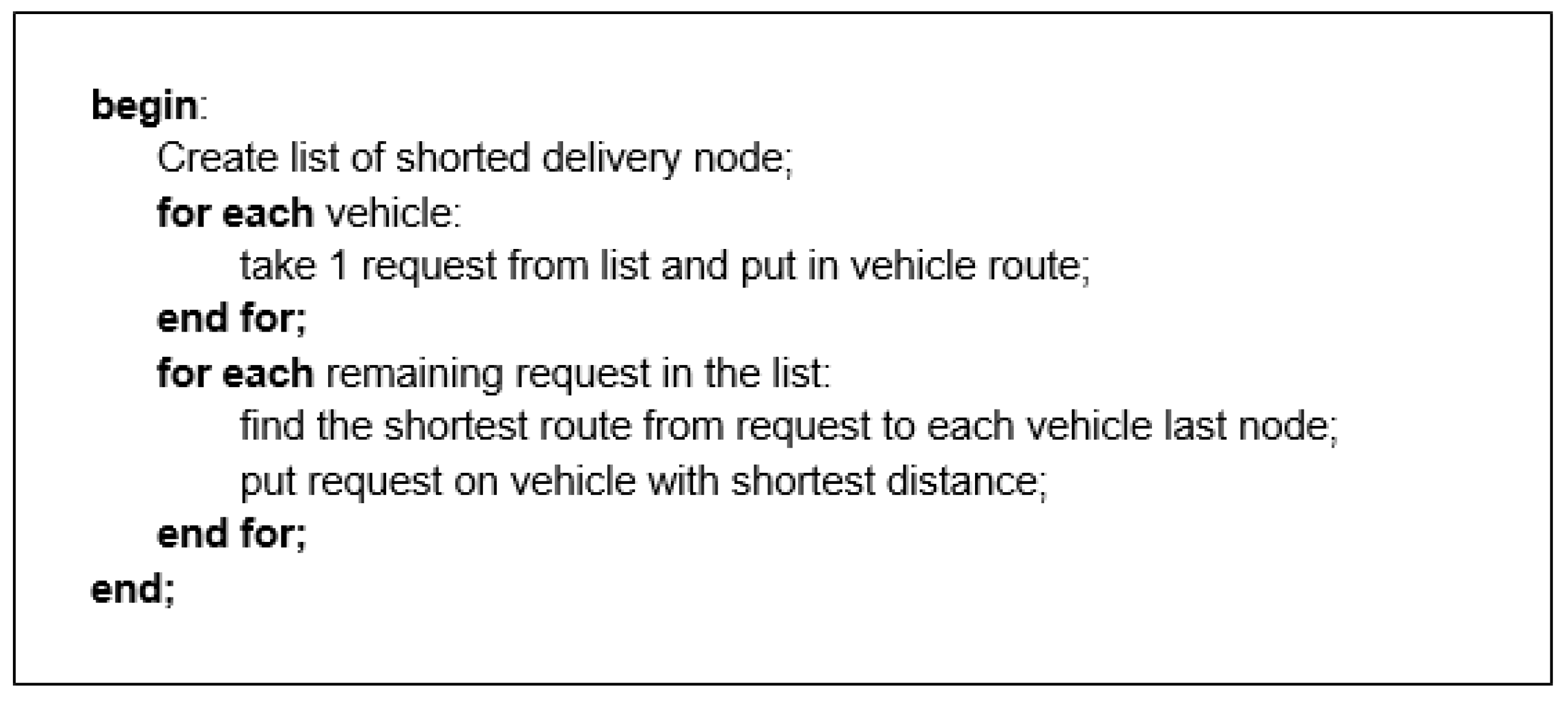
The initial solution is created using a deterministic insertion heuristic from Detti et al. [22] that is adapted to our problem. The mechanism was applied for the two arrays that represent a SARPFC solution representation. For the first array, we first created a list that consists of all delivery nodes sorted based on their latest time windows from the earliest to the latest. Second, we place the first customer node from the sorted list (pickup first, then followed by a delivery node of this customer) to the first vehicle. Third, we continue to take the second node in the sorted list and placed it to the second vehicle, and we carry on the process until all vehicles are assigned to their first customer node. Fourth, after all the vehicles are assigned the first customer, we take the next customer node in the sorted list and compare its pickup node distance to the last node in every vehicle. We put this customer node (pickup first, then followed by delivery node) to the vehicle with the shortest distance and perform this procedure until all nodes in the sorted list are assigned to a vehicle. Fifth, we then place a dummy zero at the end of every vehicle route. For the second array, a real number between 0 and 1 is randomly generated and assigned to each node, simultaneously assigning 0 for dummy zeros. Figure 2 illustrates the pseudocode of the initial solution.
3.3. Neighborhood Move
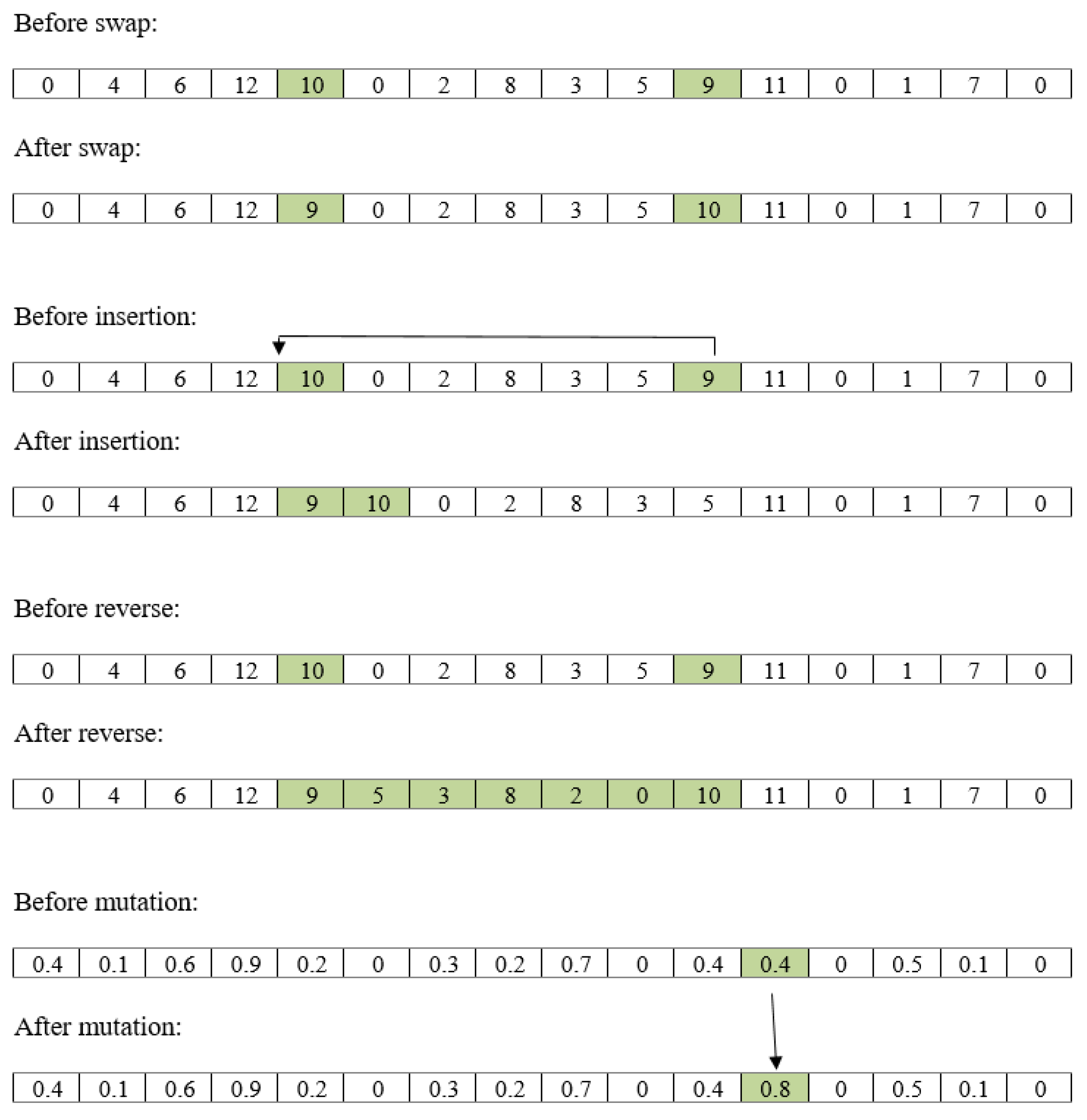
The algorithm performs one of four neighborhood moves at each iteration based on the neighborhood’s probability after the initial solution is obtained. The neighborhood moves used in the proposed SAMS are basic movements: insertion, swap, reverse, and random mutation. First, the swap move is performed by swapping two randomly chosen node positions. Second, the insertion move is made by inserting randomly chosen node j in front of randomly chosen node i. Third, the reverse move is done by reversing the order of all nodes between two randomly chosen nodes. Finally, the random mutation move replaces the randomly chosen position in the second array with a random number between 0 and 1. Figure 3 illustrates the neighborhood move.
3.4. Penalty Mechanism and Time Slack Strategy
The proposed algorithm in this research considers an infeasible solution for the evaluation process by adding a penalty for any violation of the constraint that is found while calculating the objective function value using Equation (24) as:
F(X) = c(X) − (α1T(X) + α2D(X) + α3S(X) + α4V(X) + α5W(X) + α6Z(X) + α7M(X) + α8I(X))
c(X) represents the original objective value before penalty cost is added. The penalty considered is that for violating each vehicle maximum travel time T(X), the penalty for assigning a delivery node before its pickup node D(X), the penalty for serving the same customer with a different vehicle S(X), the penalty for violating the vehicle capacity V(X), the penalty for exceeding time windows at each node W(X), the penalty for assigning two passengers consecutively in the same vehicle Z(X), the penalty for exceeding a passenger’s maximum riding time M(X), and the penalty for exceeding a maximum number of requests between particular passenger pickup and delivery request I(X). Different weights for each penalty are determined by different α values.
3.5. The Procedure of Simulated Annealing with a Mutation Strategy
In the beginning, current temperature T is set to initial temperature T0; the initial solution X is then generated. The generated initial solution X is set as the current best solution Xbest, and its objective function value obj(X) is set as the current best objective function value Fbest. At each iteration, solution X is processed by neighborhood mechanism N(X) to produce a neighborhood solution Y, and then its objective function value obj(Y) is evaluated. To decide which neighborhood move to use, the algorithm first checks if a slack time search is activated. Initially, the slack time search is not activated. Only swap, insertion, and reversion are available to be selected using the same probability. If the target temperature is reached, then a slack time search is activated, and all moves, including mutation, are available to be selected. This strategy is implemented because the slack time used in the algorithm introduces a lot of new infeasible solutions in our metaheuristic search space and affects solution quality. To mitigate this effect, the mechanism delays the slack time search to a later stage. In the proposed algorithm, a second array is used to store the slack time ratio in the solution representation. We deactivate slack time in the proposed algorithm by leaving this second array value to zero and not using mutation neighborhood moves to make sure the value stays zero.
Let Δ = obj(Y) − obj(X). If Δ is greater than zero, solution Y is better compared to previous solution X, then solution X is replaced by solution Y; otherwise, solution Y can replace solution X with a probability calculated using exp(Δ/T). When a new solution is accepted, their objective function value will be compared to the best objective function value Fbest. If the new solution is better, then we replace Fbest with its objective function value and best solution with the newly accepted solution and set the Non-improve count to 0.
After the number of current iterations reaches maximum iteration (Iiter), current temperature T is reduced by multiplying it with cooling rate α. We then increase the Non-improve count by 1. The proposed SAMS algorithm will terminate if current temperature T reaches final temperature TF or Non-improve count is bigger than Nnon-improve. Finally, the best solution and its objective function value Fbest are our final solutions. Figure 4 illustrates the proposed SA heuristics.
The SARP and its variances are difficult to solve due to the nature of the problem. Slack times used to improve the solution quality introduce a lot of infeasible solutions in the search space. The previous studies did not address this problem, which is shown in their computational time. This study employs a mutation strategy to solve SARPFC. Instead of searching slack times from the beginning of iteration, we postpone the slack time search and let the algorithm search for a good route first. Then in the middle of the search, we introduce slack time search. Moreover, we do not use repair as a diversification strategy as done in previous studies because the repair mechanism is inefficient and requires a lot of computation time.
4. The Computational Study
The computational experiment is performed on a computer equipped with an Intel® Core® i7-7700 CPU running at 3.60 GHz and 8 GB of RAM, under Windows 10 Professional operating system. The proposed SAMS algorithm is implemented in C++ and compared to CPLEX. CPLEX is a commercial solver for linear and integer programs. Moreover, the comparisons between SARP, G-SARP, and SARPFC solutions and between basic SA and SAMS are done to verify the performance of the proposed SARPFC model and SAMS algorithm. Sensitivity analyses on the SARPFC parameters are performed to provide a better understanding of the effect and benefit of flexible compartments.
4.1. Test Instances
The dataset consists of instances obtained from Yu et al. [5], which are produced using the steps and parameters provided by Li et al. [3]. Although the datasets are originally designed for the general share-a-ride problem, they can be directly adopted as SARPFC instances due to the similarity between the two problems.
4.2. Parameter Settings
Five parameters have to be set in the proposed simulated annealing—namely, α, T0, TF, Iiter, and Nnon-improve. Parameter α is a coefficient to control the annealing process. T0 and TF denote the initial temperature and final temperature, respectively. Iiter denotes the maximum number of iterations at a specific temperature. Lastly, Nnon-improve represents the maximum consecutive non-improving solution in temperature reductions. The value of each parameter will influence the quality of the result obtained from the proposed algorithm; therefore, a parameter setting experiment is conducted to get the best parameters. The following are the parameter values tested in the parameter setting:
- T0 = 8, 12, 15
- TF = 1, 0.1, 0.01
- A = 0.9, 0.99, 0.999
- Iiter = 1,000,000, 2,000,000, 3,000,000
- Nnon-improving = 5, 10, 15
Parameter setting is performed using a one factor at a time (OFAT) experiment. OFAT is performed by changing one parameter at a time while making the others fixed. The starting parameter is randomly selected as α = 0.9, T0 = 8, TF = 1, Iiter = 1,000,000, and Nnon-improve = 5. Twenty percent of the large instances are selected randomly and run four times each for every setting. The average of runs is then used to compare the result.
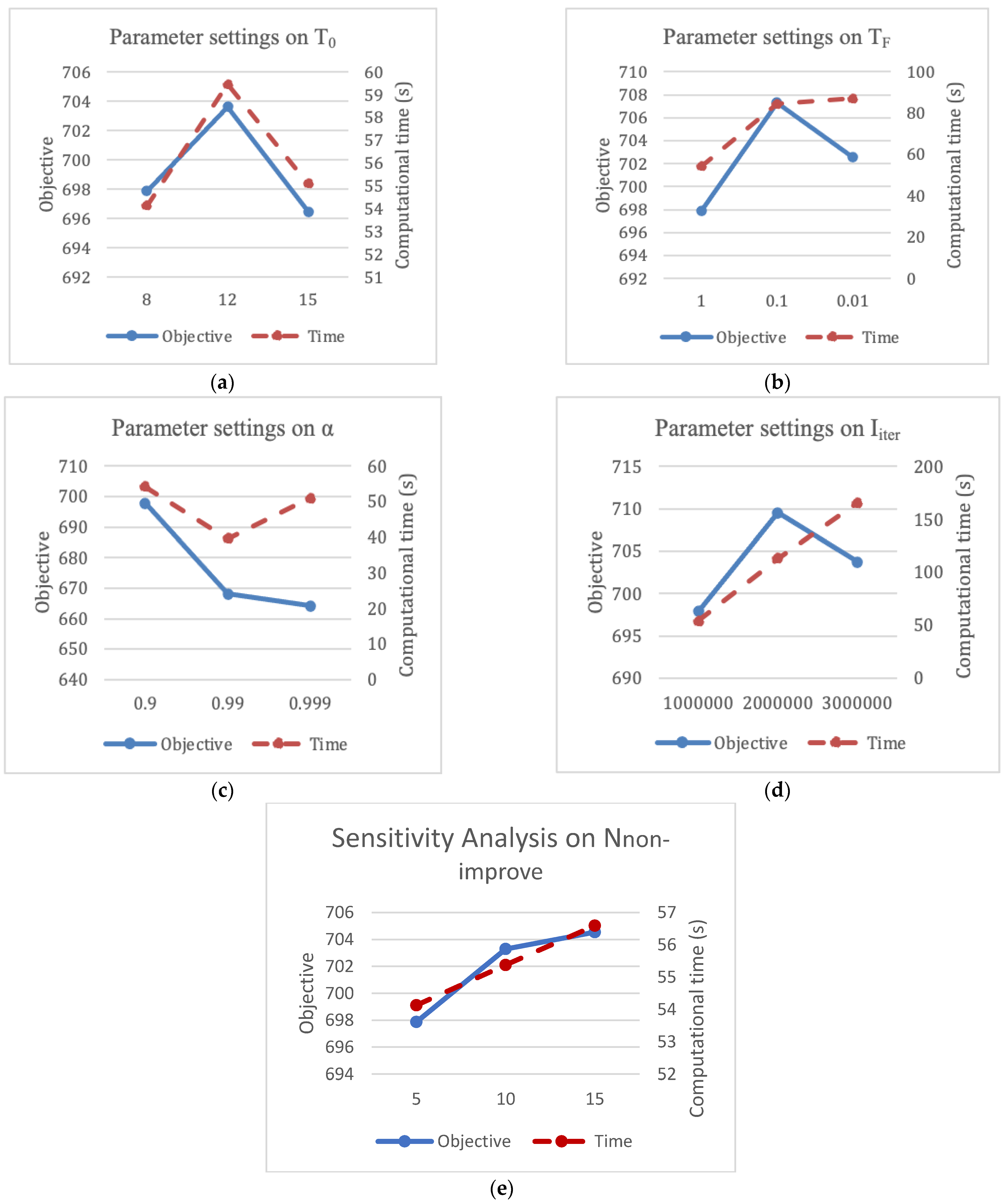
The result of the parameter setting experiment is presented in Figure 5. The blue solid line and red dashed line represent objective value and computational time, respectively. According to the result, when T0 increases, the objective value increases until T0 = 15 where it reduces. The same trend happens for computational time. For TF, it has a similar trend for the objective value to T0, but computational time seems to always increase, although the increase is not significant from TF = 0.1 to TF = 0.01. When α is increased, the objective value decreases. However, computational time decreases until α = 0.999. Computational time always increases if we increase iterations. The objective value also increases at the beginning, but it starts to decrease around Iiter = 3,000,000. The objective value and computational time increase if we increase Nnon-improve, although, at Nnon-improve = 15, the increase in objective value is not as significant as that in computational time. From OFAT, the final parameter chosen is T0 = 12, TF = 0.1, α = 0.9, Iiter = 2,000,000, and Nnon-improve = 10.
4.3. Parameter Settings on the Mutation Strategy
The proposed algorithm postpones the activation of the mutation neighborhood move at a later stage of the algorithm. Therefore, we need to find when is the best time to activate it by using sensitivity analysis. We study six possible times to activate the slack time search: at the beginning (0% of initial temperature reduction), 15% of initial temperature reduction, 30% of initial temperature reduction, 45% of initial temperature reduction, 60% of initial temperature reduction, and 75% of initial temperature reduction. Activation at the beginning indicates that we activate it directly or at T0, while 15% of initial temperature reduction means we activate it after current temperature T reaches T0 × (1–15%). Figure 6 shows the parameter setting results for slack time. The results show that the objective value increases each time the delay on slack time activation increases until we delay it to a 45% reduction in T0. Objectives start to drop at a 60% reduction. This may be because there is not enough time to explore slack time in the search space.
4.4. Comparison between SAMS and CPLEX
To verify the performance of the proposed SAMS, SARPFC instances are solved using CPLEX and the proposed SAMS algorithm, and then the results are compared. The algorithm’s performance is measured in terms of the percentage gap between the SAMS solution value and the optimal solution value obtained by CPLEX. CPLEX and the proposed algorithm are able to obtain the optimal solution to each instance. The results of all instances for both approaches appear in Table 1.
The results show that both CPLEX and the proposed SAMS algorithm can solve the SARPFC instances to optimality. The proposed SAMS finds the optimal solution with a shorter computational time for some instances. The algorithm is also tested on SARP to see if it performs better than other algorithms in the literature.
The proposed SAMS is quite robust. With a little bit of modification in the way it reads the solution representation, it can solve SARP. Table 2 shows the results of solving small SARP instances using CPLEX and SA reported by Yu et al. [5] and the proposed SAMS. The results present that both SA and SAMS can obtain the optimal solution, where the average computational time of SAMS and SA is 0.014 and 0.993 min, respectively. Gap 1 represents the difference in objective value for the CPLEX result and SAMS result, while Gap 2 represents the difference in objective value for the results of SA and SAMS. In summary, SAMS can lead to the optimal solution for both small SARP and SARPFC instances. This result shows that the proposed SAMS algorithm can solve both models with good performance and competitive computational time.
For larger instances, the result from SAMS is compared to that of SA because CPLEX is unable to find a solution within a reasonable time allocation. Table 3 shows the comparison of results obtained by these two algorithms. According to the results, the proposed SAMS outperforms the SA result by obtaining 20 new best solutions for all the 20 instances. The gap ranges from 24.71% to 618.51%. This shows that the proposed SAMS is superior compared to the SA algorithm in terms of solution quality.
4.5. Comparison between Basic SA and SAMS for SARPFC
This section provides the analysis of results obtained by the basic SA and SAMS for solving SARPFC. It is performed to identify the benefit of the mutation strategy in the proposed SAMS for SARPFC. The results in Table 4 show that the basic SA is not able to find feasible solutions for four instances (namely, instances Pr08, Pr09, Pr10, and Pr20). The mutation strategy in the proposed algorithms gives an average of 3.65% increase in solution quality for all feasible solutions found by the basic SA and also improves the algorithm performance to obtain solutions for all instances.
4.6. Comparison between SARP, G-SARP, and SARPFC
This section presents a comparison between SARP, G-SARP, and SARPFC solutions. All models aim to obtain the highest possible profit from serving all customers. This comparative study intends to provide insight to the taxi operators to decide which application to use to increase their profit from the existing taxi network.
4.6.1. Comparison of Small Instances
SARPFC is a SARP extension that considers flexible compartments in taxi service, while in G-SARP, a taxi is allowed to carry more than one passenger simultaneously. Yu et al. [5] solve G-SARP using a modified SA that uses two mechanisms to deal with infeasible solutions. The first one is the penalty for infeasibility, and the second is the repair mechanism. They search slack times starting from the beginning of iteration. This method results in a slower computational time. Table 5 shows a comparison between SARP, G-SARP, and SARPFC solutions for small instances. Gap 1 represents the difference between SARPFC and SARP solutions, while Gap 2 represents the difference between SARPFC and G-SARP solutions. Positive gaps indicate SARPFC is better, while negative ones indicate it is worse. As mentioned earlier, this result is the optimal solution. The gap between SARP and SARPFC is minimal due to the very small number of customers. Hence, only an average of 0.07% improvement is obtained. The gap between SARPFC and G-SARP shows a negative value. This means that G-SARP produces a better solution (higher profit) compared to SARPFC. The G-SARP approach shows that allowing multiple passengers to ride taxis at the same time, and the higher passenger fare than that of the parcel fare, increase the profit compared to the SARPFC approach. However, the analysis taken from small-size instances may not represent the general picture of the situation. Therefore, a comparison on large instances is conducted.
4.6.2. A Comparison of Large Instances
Table 6 presents a comparison between SARP, G-SARP, and SARPFC solutions for large instances. Gap 1 shows that compared to SARP, SARPFC finds better solutions, where most solutions are larger than those by SARP with an average of 2.27% increase in profit. The small improvement reflected in gap 1 is affected by the selection of compartment size in the instances. The large instances are assumed to use a large-size taxi with a six-seat passenger capacity. Thus, compartment size flexibility in SARPFC is not improved much. The further analysis of compartment size is discussed in the next section. The result from gap 2 shows a different finding from the result for the small instances.
Table 6 shows that SARPFC results are better than G-SARP results, with an average improvement gap of 44.39%. The increasing number of passenger requests and parcel requests for the large instances contribute to higher profit in SARPFC. Concurrently, the G-SARP advantage that relies on a distance saving result by shared passenger services is not effective for this particular dataset since it also increases the penalty cost for a passenger’s extra riding time compared to that by direct driving.
4.7. Sensitivity Analysis on the Number of Parcel Requests and Compartment Size
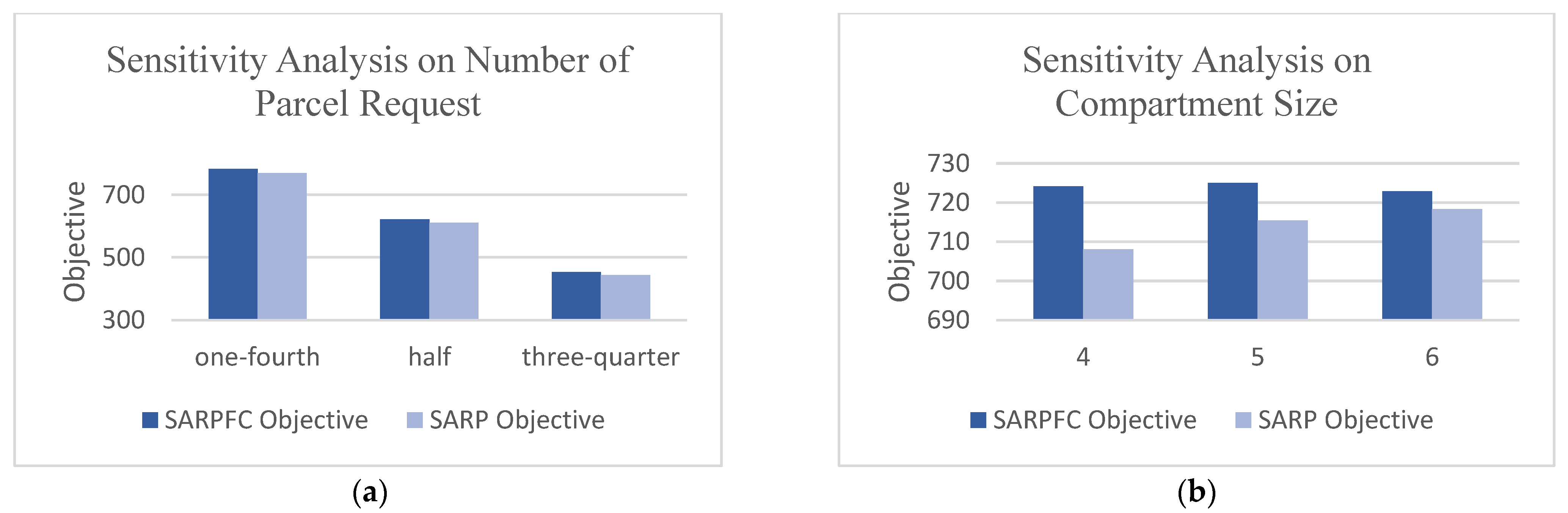
The first sensitivity analysis is on the impact of the percentage of parcel requests among total requests on the total profit generated by the systems. For this experiment, we conduct three scenarios where the number of parcel requests is set to 1/4, 2/4, and 3/4 out of the total requests and set compartment size constant at 6. Figure 7a shows that the profit generated in both SARP and SARPC decreases with an increase in the number of parcel requests. This situation appears mainly because the contribution of the passenger fare to the total profit is higher than the contribution of parcel fare to the total profit. However, the objective function of the SARPFC model is shown to be consistently better than that of SARP, which supports the flexibility in which sharing compartments can have a slight advantage in terms of total generated profit.
The second sensitivity analysis is on the impact of compartment size on the total profit generated by the systems. To perform this task, we conduct a computational experiment in which the compartment size is set to be 4, 5, and 6, and 1/3 of the requests are parcel requests. From the perspective of a practical situation, the instance used in the previous experiment takes a compartment size of 6, which is comparable to a family taxi that has 6 passenger seats. This kind of taxi is less common compared to taxis with only 4 passenger seats.
Figure 7b shows the objective value of SARP and SARPFC with the compartment sizes of 4, 5, and 6, according to which the profit generated for each compartment size in SARPFC is not much different from the other. At the same time, increasing the compartment size tends to increase the number of profits generated in SARP. The results show a clear influence on compartment size. Due to SARPFC’s flexibility in using the passenger seat to store parcels, the possibility for any compartment size to go over capacity is low. We thus infer that using a smaller size vehicle (with a smaller compartment) can achieve a similar benefit to using a larger vehicle. However, this flexibility does not apply in SARP. Thus, the size of the compartment may need to be increased to gain a similar potential benefit.
5. Conclusions and Future Research
This research introduces the SARPFC and formulates a mathematical model for the problem. This model introduces the flexibility of adjusting compartments not only for each vehicle or route, but also for every visited node based on demand. This feature increases the flexibility of the model to service more parcels and fully utilizes vehicle compartments. A simulated annealing (SA) algorithm with a mutation strategy is proposed to solve the problem. The mutation strategy is a mechanism to reduce the number of infeasible solutions in the search process. The algorithm was tested on small instances and compared to solutions obtained from CPLEX and on large instances compared to the algorithm in the literature.
A thorough computational analysis involved a preliminary experiment, algorithm verification, comparison with various SARP variants, and sensitivity analysis. In the preliminary experiment, the best parameter combination for the proposed SAMS algorithm was obtained using the one factor at a time method. The algorithm verification results show that the proposed SAMS outperforms the SA result by obtaining 20 new best solutions from 20 instances. The average gap between the results of the two algorithms is 73.71%, suggesting that the proposed SAMS is superior compared to the SA algorithm in terms of solution quality. A comparison with SARP variants provides the insight that SARPFC can have the advantage in terms of the total profit generated by the system. A sensitivity analysis was also performed to assess the effects of the portion of parcel requests among the total requests and the compartment size on the objective function. The profit is reduced if there are more package requests compared to more passengers due to higher passenger fares. Flexible compartments in SARPFC allow a taxi to accrue higher profit with only a small taxi (four-compartment sedan taxi) compared to SARP where a six-compartment size is used (family MVP taxi).
For future research, an extension that considers both the ride-sharing of passengers in G-SARP and the flexible compartments of this research can be examined. Considering passenger comfort while riding in an appropriate route is also an interesting future research topic. Lastly, because SARPFC has many infeasible solutions in the search space, it is necessary to develop an algorithm that can more efficiently solve the problem.
Author Contributions
Conceptualization, V.F.Y.; data curation, P.A.Y.I.; formal analysis, P.A.Y.I.; funding acquisition, V.F.Y. and S.-W.L.; investigation, P.A.Y.I.; methodology, P.A.Y.I. and A.A.N.P.R.; project administration, V.F.Y.; resources, V.F.Y. and P.A.Y.I.; software, P.A.Y.I. and A.A.N.P.R.; supervision, V.F.Y. and S.-W.L.; validation, V.F.Y., P.A.Y.I., A.A.N.P.R. and S.-W.L.; visualization, P.A.Y.I.; writing—original draft preparation, V.F.Y. and P.A.Y.I.; writing—review and editing, V.F.Y., P.A.Y.I., A.A.N.P.R. and S.-W.L. All authors have read and agreed to the published version of the manuscript.
Funding
This research is partially supported by the Ministry of Science and Technology, Taiwan, under Grant MOST 106-2410-H-011-002-MY3, and the Center for Cyber-Physical System Innovation from The Featured Areas Research Center Program within the framework of the Higher Education Sprout Project by the Ministry of Education (MOE) in Taiwan. The work of the fourth author is supported in part by the Ministry of Science and Technology, Taiwan, under Grant MOST 109-2410-H-182-009MY3, and the Linkou Chang Gung Memorial Hospital under Grant BMRPA19.
Institutional Review Board Statement
Not applicable.
Informed Consent Statement
Not applicable.
Data Availability Statement
Not applicable.
Acknowledgments
This research was partially supported by the Ministry of Science and Technology of the Republic of China (Taiwan) under grant MOST 106-2410-H-011-002-MY3 and the Center for Cyber-Physical System Innovation from the Featured Areas Research Center Program within the framework of the Higher Education Sprout Project by the Ministry of Education (MOE) in Taiwan. The work of S.-W. Lin was supported in part by the Ministry of Science and Technology, Taiwan, under Grant MOST 109-2410-H-182-009MY3, and in part by the Linkou Chang Gung Memorial Hospital under Grant BMRPA19.
Conflicts of Interest
The authors declare no conflict of interest.
References
- Cordeau, J.-F.; Laporte, G. The dial-a-ride problem: Models and algorithms. Ann. Oper. Res. 2007, 153, 29–46. [Google Scholar] [CrossRef]
- Savelsbergh, M.W.; Sol, M. The general pickup and delivery problem. Transp. Sci. 1995, 29, 17–29. [Google Scholar] [CrossRef] [Green Version]
- Li, B.; Krushinsky, D.; Reijers, H.A.; Van Woensel, T. The share-a-ride problem: People and parcels sharing taxis. Eur. J. Oper. Res. 2014, 238, 31–40. [Google Scholar] [CrossRef] [Green Version]
- Li, B.; Krushinsky, D.; Van Woensel, T.; Reijers, H.A. The Share-a-Ride problem with stochastic travel times and stochastic delivery locations. Transp. Res. Part C Emerg. Technol. 2016, 67, 95–108. [Google Scholar] [CrossRef]
- Yu, V.F.; Purwanti, S.S.; Redi, A.A.N.P.; Lu, C.-C.; Suprayogi, S.; Jewpanya, P. Simulated annealing heuristic for the general share-a-ride problem. Eng. Optim. 2018, 50, 1178–1197. [Google Scholar] [CrossRef]
- Beirigo, B.A.; Schulte, F.; Negenborn, R.R. Integrating people and freight transportation using shared autonomous vehicles with compartments. IFAC-Pap. 2018, 51, 392–397. [Google Scholar] [CrossRef]
- Do, P.-T.; Nguyen, N.-Q.; Pham, Q.-D. A time-dependent model with speed windows for share-a-ride problems: A case study for Tokyo transportation. Data Knowl. Eng. 2018, 114, 67–85. [Google Scholar]
- Cavagnini, R.; Morandi, V. Implementing Horizontal Cooperation in Public Transport and Parcel Deliveries: The Cooperative Share-A-Ride Problem. Sustainability 2021, 13, 4362. [Google Scholar] [CrossRef]
- Ostermeier, M.; Henke, T.; Hübner, A.; Wäscher, G. Multi-Compartment Vehicle Routing Problems: State-of-the-art, Modeling Framework and Future Directions. Eur. J. Oper. Res. 2021, 292, 799–817. [Google Scholar] [CrossRef]
- Hsu, Y.C.; Walteros, J.L.; Batta, R. Solving the petroleum replenishment and routing problem with variable demands and time windows. Ann. Oper. Res. 2020, 294, 9–46. [Google Scholar] [CrossRef]
- Rabbani, M.; Farrokhi-Asl, H.; Asgarian, B. Solving a bi-objective location routing problem by a NSGA-II combined with clustering approach: Application in waste collection problem. J. Ind. Eng. Int. 2017, 13, 13–27. [Google Scholar] [CrossRef] [Green Version]
- Chen, L.; Liu, Y.; Langevin, A. A multi-compartment vehicle routing problem in cold-chain distribution. Comput. Oper. Res. 2019, 111, 58–66. [Google Scholar]
- Lahyani, R.; Coelho, L.C.; Khemakhem, M.; Laporte, G.; Semet, F. A multi-compartment vehicle routing problem arising in the collection of olive oil in Tunisia. Omega 2015, 51, 1–10. [Google Scholar] [CrossRef]
- Christiansen, M.; Fagerholt, K.; Rachaniotis, N.P.; Stålhane, M. Operational planning of routes and schedules for a fleet of fuel supply vessels. Transp. Res. Part E Logist. Transp. Rev. 2017, 105, 163–175. [Google Scholar]
- Siswanto, N.; Wiratno, S.E.; Rusdiansyah, A.; Sarker, R. Maritime inventory routing problem with multiple time windows. J. Ind. Manag. Optim. 2019, 15, 1185. [Google Scholar] [CrossRef]
- Li, B.; Krushinsky, D.; Van Woensel, T.; Reijers, H.A. An adaptive large neighborhood search heuristic for the share-a-ride problem. Comput. Oper. Res. 2016, 66, 170–180. [Google Scholar] [CrossRef] [Green Version]
- Silvestrin, P.V.; Ritt, M. An iterated tabu search for the multi-compartment vehicle routing problem. Comput. Oper. Res. 2017, 81, 192–202. [Google Scholar] [CrossRef]
- Yu, V.F.; Jewpanya, P.; Redi, A.A.N.P.; Tsao, Y.-C. Adaptive neighborhood simulated annealing for the heterogeneous fleet vehicle routing problem with multiple cross-docks. Comput. Oper. Res. 2021, 129, 105205. [Google Scholar] [CrossRef]
- Yahyaoui, H.; Kaabachi, I.; Krichen, S.; Dekdouk, A. Two metaheuristic approaches for solving the multi-compartment vehicle routing problem. Oper. Res. 2018, 20, 2085–2108. [Google Scholar] [CrossRef] [Green Version]
- Abdulkader, M.M.; Gajpal, Y.; ElMekkawy, T.Y. Hybridized ant colony algorithm for the multi compartment vehicle routing problem. Appl. Soft Comput. 2015, 37, 196–203. [Google Scholar] [CrossRef]
- Goodson, J.C. A priori policy evaluation and cyclic-order-based simulated annealing for the multi-compartment vehicle routing problem with stochastic demands. Eur. J. Oper. Res. 2015, 241, 361–369. [Google Scholar] [CrossRef]
- Detti, P.; Papalini, F.; de Lara, G.Z.M. A multi-depot dial-a-ride problem with heterogeneous vehicles and compatibility constraints in healthcare. Omega 2017, 70, 1–14. [Google Scholar] [CrossRef]
Figure 1.
Illustration of solution representation for SARPFC.

Figure 2.
A pseudocode of the initial solution.

Figure 3.
An illustration of swap, insertion, reverse, and mutation moves.

Figure 4.
A flowchart of Simulated Annealing with Mutation Strategy (SAMS).

Figure 5.
The impact of simulated annealing parameters on the quality of share-a-ride problem with flexible compartments solution and computational time on (a) T0 parameter, (b) TF parameter, (c) α parameter, (d) Iiter parameter, and (e) Nnon-improving parameter.
Figure 5.
The impact of simulated annealing parameters on the quality of share-a-ride problem with flexible compartments solution and computational time on (a) T0 parameter, (b) TF parameter, (c) α parameter, (d) Iiter parameter, and (e) Nnon-improving parameter.

Figure 6.
Parameter settings on slack time.

Figure 7.
Sensitivity analysis: (a) impact of the number of parcel request on solution quality and (b) impact of compartment size on solution quality.
Figure 7.
Sensitivity analysis: (a) impact of the number of parcel request on solution quality and (b) impact of compartment size on solution quality.


Table 1.
Comparison between CPLEX and proposed SAMS solution for SARPFC.
| Instance | CPLEX | SAMS | Gap a (%) | ||
|---|---|---|---|---|---|
| Objective | Time (m) | Objective | Time (m) | ||
| instance14 | 59.24 | 0.010 | 59.24 | 0.005 | 0.00 |
| instance14n | 56.94 | 0.001 | 56.94 | 0.005 | 0.00 |
| instance24 | 13.11 | 0.007 | 13.11 | 0.005 | 0.00 |
| instance24n | 13.73 | 0.004 | 13.73 | 0.009 | 0.00 |
| instance16 | 85.08 | 0.102 | 85.08 | 0.009 | 0.00 |
| instance16n | 64.77 | 0.001 | 64.77 | 0.006 | 0.00 |
| instance26 | 78.39 | 0.751 | 78.39 | 0.008 | 0.00 |
| instance26n | 51.15 | 0.020 | 51.15 | 0.011 | 0.00 |
a Gap = (obj of SAMS − obj of CPLEX)/obj of CPLEX × 100%.
Table 2.
Comparison between CPLEX, proposed SAMS, and SA solution for SARP small instance.
| Instance | CPLEX | SAMS | SA | Gap 1 a (%) | Gap 2 b (%) | |||
|---|---|---|---|---|---|---|---|---|
| Objective | Time (m) | Objective | Time (m) | Objective | Time (m) | |||
| instance14 | 58.93 | 0.010 | 58.93 | 0.003 | 58.93 | 0.921 | 0.00 | 0.00 |
| instance14n | 56.94 | 0.002 | 56.94 | 0.003 | 56.94 | 0.902 | 0.00 | 0.00 |
| instance24 | 13.11 | 0.007 | 13.11 | 0.020 | 13.11 | 1.070 | 0.00 | 0.00 |
| instance24n | 13.73 | 0.005 | 13.73 | 0.021 | 13.73 | 0.063 | 0.00 | 0.00 |
| instance16 | 85.04 | 0.193 | 85.04 | 0.035 | 85.04 | 0.066 | 0.00 | 0.00 |
| instance16n | 64.77 | 0.003 | 64.77 | 0.006 | 64.77 | 4.651 | 0.00 | 0.00 |
| instance26 | 78.39 | 0.167 | 78.39 | 0.021 | 78.39 | 0.079 | 0.00 | 0.00 |
| instance26n | 51.15 | 0.026 | 51.15 | 0.005 | 51.15 | 0.196 | 0.00 | 0.00 |
a Gap 1 = (obj of SAMS − obj of CPLEX)/obj of CPLEX × 100%. b Gap 2 = (obj of SAMS − obj of SA)/obj of SA × 100%.
Table 3.
Comparison between proposed SAMS and SA solution for SARP large instance.
| Instance | SAMS | SA | Gap a (%) | ||
|---|---|---|---|---|---|
| Objective | Time (m) | Objective | Time (m) | ||
| Pr01 | 257.012 | 0.288 | 35.77 | 2.193 | 618.51 |
| Pr02 | 393.79 | 1.153 | 315.753 | 21.938 | 24.71 |
| Pr03 | 868.938 | 1.520 | 597.513 | 74.42 | 45.43 |
| Pr04 | 948.741 | 2.329 | 667.912 | 53.344 | 42.05 |
| Pr05 | 1144.29 | 2.951 | 779.238 | 102.925 | 46.85 |
| Pr06 | 1368.94 | 3.567 | 1055.004 | 120.348 | 29.76 |
| Pr07 | 404.266 | 0.919 | 246.681 | 14.625 | 63.88 |
| Pr08 | 767.634 | 1.858 | 571.333 | 18.386 | 34.36 |
| Pr09 | 1131.71 | 2.711 | 865.26 | 126.892 | 30.79 |
| Pr10 | 1570.78 | 11.733 | 1065.457 | 130.936 | 47.43 |
| Pr11 | 269.625 | 0.979 | 124.321 | 18.386 | 116.88 |
| Pr12 | 409.451 | 1.689 | 312.485 | 35.398 | 31.03 |
| Pr13 | 894.306 | 2.301 | 591.676 | 118.113 | 51.15 |
| Pr14 | 1014.6 | 2.936 | 706.884 | 44.58 | 43.53 |
| Pr15 | 1193.11 | 3.586 | 879.228 | 209.834 | 35.70 |
| Pr16 | 1461.89 | 4.322 | 1131.676 | 172.807 | 29.18 |
| Pr17 | 422.137 | 1.324 | 266.287 | 13.928 | 58.53 |
| Pr18 | 813.039 | 2.294 | 553.26 | 16.904 | 46.95 |
| Pr19 | 1187.2 | 3.435 | 824.384 | 68.782 | 44.01 |
| Pr20 | 1585.56 | 4.731 | 1188.861 | 244.671 | 33.37 |
a Gap = (obj of SAMS − obj of SA)/obj of SA × 100%.
Table 4.
Comparison between basic SA and proposed SAMS solution for SARPFC large instance.
| Instance | SAMS | SA | Gap a (%) | ||
|---|---|---|---|---|---|
| Objective | Time (m) | Objective | Time (m) | ||
| Pr01 | 268.776 | 1.333 | 246.723 | 0.893 | 8.94 |
| Pr02 | 411.212 | 2.525 | 402.192 | 2.264 | 2.24 |
| Pr03 | 896.427 | 3.602 | 844.105 | 3.500 | 6.20 |
| Pr04 | 985.085 | 4.554 | 954.085 | 5.298 | 3.25 |
| Pr05 | 1170.06 | 6.045 | 1159.17 | 6.317 | 0.94 |
| Pr06 | 1396.82 | 6.762 | 1363.46 | 8.171 | 2.45 |
| Pr07 | 420.003 | 1.992 | 398.368 | 1.503 | 5.43 |
| Pr08 | 803.332 | 3.611 | - | - | - |
| Pr09 | 1098.69 | 3.046 | - | - | - |
| Pr10 | 1539.92 | 7.276 | - | - | - |
| Pr11 | 271.409 | 1.242 | 264.599 | 1.344 | 2.57 |
| Pr12 | 426.12 | 2.701 | 411.537 | 2.574 | 3.54 |
| Pr13 | 911.628 | 3.635 | 883.428 | 3.704 | 3.19 |
| Pr14 | 1037.92 | 5.081 | 1007.45 | 5.627 | 3.02 |
| Pr15 | 1210.26 | 6.245 | 1160.47 | 6.421 | 4.29 |
| Pr16 | 1483.36 | 7.636 | 1412.39 | 7.988 | 5.02 |
| Pr17 | 426.742 | 2.245 | 410.325 | 1.584 | 4.00 |
| Pr18 | 861.319 | 3.957 | 819.149 | 3.936 | 5.15 |
| Pr19 | 1190.68 | 5.696 | 1180.01 | 5.910 | 0.90 |
| Pr20 | 1620.52 | 7.677 | - | - | - |
a Gap = (obj of SAMS − obj of SA)/obj of SA × 100%.
Table 5.
Comparison between SARP, G-SARP, and SARPFC solution for small instance.
| Instance | SARP | G-SARP | SARPFC | Gap 1 a (%) | Gap 2 b (%) | |||
|---|---|---|---|---|---|---|---|---|
| Objective | Time (m) | Objective | Time (m) | Objective | Time (m) | |||
| instance14 | 58.93 | 0.921 | 70.413 | 1.220 | 59.24 | 0.005 | 0.53 | −15.87 |
| instance14n | 56.94 | 0.902 | 56.943 | 1.554 | 56.94 | 0.005 | 0.00 | −0.01 |
| instance24 | 13.11 | 1.070 | 16.673 | 1.521 | 13.11 | 0.005 | 0.00 | −21.37 |
| instance24n | 13.73 | 0.063 | 16.68 | 2.623 | 13.73 | 0.009 | 0.00 | −17.69 |
| instance16 | 85.05 | 0.066 | 94.589 | 0.076 | 85.08 | 0.009 | 0.04 | −10.05 |
| instance16n | 64.77 | 4.651 | 73.957 | 0.108 | 64.77 | 0.006 | 0.00 | −12.42 |
| instance26 | 78.39 | 0.079 | 79.861 | 0.085 | 78.39 | 0.008 | 0.00 | −1.84 |
| instance26n | 51.15 | 0.196 | 58.901 | 0.194 | 51.15 | 0.011 | 0.00 | −13.16 |
a Gap 1 = (obj of SAMS − obj of SARP)/obj of SARP × 100%. b Gap 2 = (obj of SAMS − obj of G-SARP)/obj of G-SARP × 100%.
Table 6.
Comparison between SARP, G-SARP, and SARPFC solution for large instances.
| Instance | SARP | G-SARP | SARPFC | Gap 1 a (%) | Gap 2 b (%) | |||
|---|---|---|---|---|---|---|---|---|
| Obj. | Time (m) | Obj | Time (m) | Obj | Time (m) | |||
| Pr01 | 257.012 | 0.288 | 138.667 | 5.262 | 268.776 | 1.333 | 4.58 | 93.83 |
| Pr02 | 393.79 | 1.153 | 329.168 | 20.312 | 411.212 | 2.525 | 4.42 | 24.92 |
| Pr03 | 868.938 | 1.520 | 584.259 | 66.739 | 896.427 | 3.602 | 3.16 | 53.43 |
| Pr04 | 948.741 | 2.329 | 702.299 | 122.282 | 985.085 | 4.554 | 3.83 | 40.27 |
| Pr05 | 1144.29 | 2.951 | 812.518 | 210.991 | 1170.06 | 6.045 | 2.25 | 44.00 |
| Pr06 | 1368.94 | 3.567 | 1055.004 | 286.152 | 1396.82 | 6.762 | 2.04 | 32.40 |
| Pr07 | 404.266 | 0.919 | 243.043 | 9.495 | 420.003 | 1.992 | 3.89 | 72.81 |
| Pr08 | 767.634 | 1.858 | 635.713 | 44.742 | 803.332 | 3.611 | 4.65 | 26.37 |
| Pr09 | 1131.71 | 2.711 | 899.202 | 152.515 | 1098.69 | 3.046 | -2.92 | 22.19 |
| Pr10 | 1570.78 | 11.733 | 1138.045 | 269.434 | 1539.92 | 7.276 | -1.96 | 35.31 |
| Pr11 | 269.625 | 0.979 | 138.968 | 7.223 | 271.409 | 1.242 | 0.66 | 95.30 |
| Pr12 | 409.451 | 1.689 | 329.171 | 40.768 | 426.12 | 2.701 | 4.07 | 29.45 |
| Pr13 | 894.306 | 2.301 | 589.101 | 73.033 | 911.628 | 3.635 | 1.94 | 54.75 |
| Pr14 | 1014.6 | 2.936 | 761.957 | 135.608 | 1037.92 | 5.081 | 2.30 | 36.22 |
| Pr15 | 1193.11 | 3.586 | 879.228 | 270.463 | 1210.26 | 6.245 | 1.44 | 37.65 |
| Pr16 | 1461.89 | 4.322 | 1131.676 | 275.332 | 1483.36 | 7.636 | 1.47 | 31.08 |
| Pr17 | 422.137 | 1.324 | 277.027 | 14.955 | 426.742 | 2.245 | 1.09 | 54.04 |
| Pr18 | 813.039 | 2.294 | 700.252 | 71.952 | 861.319 | 3.957 | 5.94 | 23.00 |
| Pr19 | 1187.2 | 3.435 | 824.384 | 152.859 | 1190.68 | 5.696 | 0.29 | 44.43 |
| Pr20 | 1585.56 | 4.731 | 1188.861 | 278.737 | 1620.52 | 7.677 | 2.20 | 36.31 |
a Gap 1 = (obj of SARPFC − obj of SARP)/obj of SARP × 100%. b Gap 2 = (obj of SARPFC − obj of G-SARP)/obj of G-SARP × 100%.
Publisher’s Note: MDPI stays neutral with regard to jurisdictional claims in published maps and institutional affiliations. |
© 2021 by the authors. Licensee MDPI, Basel, Switzerland. This article is an open access article distributed under the terms and conditions of the Creative Commons Attribution (CC BY) license (https://creativecommons.org/licenses/by/4.0/).
Share and Cite
MDPI and ACS Style
Yu, V.F.; Indrakarna, P.A.Y.; Redi, A.A.N.P.; Lin, S.-W. Simulated Annealing with Mutation Strategy for the Share-a-Ride Problem with Flexible Compartments. Mathematics 2021, 9, 2320. https://0-doi-org.brum.beds.ac.uk/10.3390/math9182320
AMA Style
Yu VF, Indrakarna PAY, Redi AANP, Lin S-W. Simulated Annealing with Mutation Strategy for the Share-a-Ride Problem with Flexible Compartments. Mathematics. 2021; 9(18):2320. https://0-doi-org.brum.beds.ac.uk/10.3390/math9182320
Chicago/Turabian StyleYu, Vincent F., Putu A. Y. Indrakarna, Anak Agung Ngurah Perwira Redi, and Shih-Wei Lin. 2021. "Simulated Annealing with Mutation Strategy for the Share-a-Ride Problem with Flexible Compartments" Mathematics 9, no. 18: 2320. https://0-doi-org.brum.beds.ac.uk/10.3390/math9182320
Note that from the first issue of 2016, this journal uses article numbers instead of page numbers. See further details here.