The Polynomial Least Squares Method for Nonlinear Fractional Volterra and Fredholm Integro-Differential Equations

Abstract

We present a relatively new and very efficient method to find approximate analytical solutions for a very general class of nonlinear fractional Volterra and Fredholm integro-differential equations. The test problems included and the comparison with previous results by other methods clearly illustrate the simplicity and accuracy of the method.

1. Introduction

The two mathematicians Vito Volterra and Erik Ivar Fredholm, through their works published in the early 1900s, laid the foundations of the modern theory of integro-differential equations. As the fractional Volterra and Fredholm integro-differential equations have multiple applications in various fields such as engineering, physics, mechanics, etc., they have aroused the interest of many researchers.

In recent years there have been numerous papers in which, for equations of this type, approximate analytical solutions or numerical solutions by various methods are presented, and this is because obtaining an exact solution is often impossible.

Among the methods used to compute approximate analytical and numerical solutions for fractional Volterra and Fredholm integro-differential equations we mention:

• The Homotopy Perturbation Method, used by Ghasemi et al. in 2007 ([1])to solve nonlinear integro-differential equations and by Dheghan and Shakeri in 2008 ([2]) to solve integro-differential equation with time-periodic coefficients,
• The Bernoulli Matrix Method, used by Bhrawya et al. in 2012 ([3]) to find solutions for fractional Fredholm integro-differential equations, by Keshavarz et al. in 2019 ([4]) to find solutions for a class of nonlinear mixed Fredholm–Volterra integro-differential equations of fractional order and by Rajagopal et al. in 2020 ([5]) to find solutions for fractional-order Volterra integro-differential equations,
• The Legendre Wavelets Method, employed by Meng et al. in 2014 ([6]) to solve Volterra–Fredholm integro-differential equations of fractional order,
• The Legendre Spectral Element Method, employed by Lotfi and Alipanah in 2020 (([7]) to solve Volterra–Fredholm integro-differential equations,
• The Shifted Jacobi-Spectral Collocation Method, used by Al-Safi in 2018 ([8]) to solve Volterra–Fredholm integro-differential equations of fractional order,
• The Reproducing Kernel Hilbert Space Method, used by Arkub et al. in 2013 ([9]) to solve Fredholm integro-differential equations,
• The Sinc-Collocation Method, used by Alkan and Hatipoglu in 2017 ([10]) to solve Volterra–Fredholm integro-differential equations of fractional order,
• The Legendre Collocation Method, employed by Rohaninasab et al. in 2017 ([11]) to solve high-order linear Volterra–Fredholm integro-differential equations,
• The Adomian Decomposition Method, used by Momani and Noor in 2006 ([12]) and by Farhood in 2015 ([13]),
• The Shifted Chebyshev Polynomials Method, also used by Farhood in 2015 ([13]) to find solutions for nonlinear fractional integro-differential equations,
• The Genocchi Polynomials Method, employed by Loh et al. in 2017 ([14]) to solve Volterra–Fredholm integro-differential equations of fractional order,
• The Euler Wavelets Method, used by Wang and Zhu in 2017 ([15]) to find approximate solutions for Fredholm–Volterra fractional integro-differential equations,
• The Lucas Wavelets Method, employed by Dehestani et al. in 2021 ([16]) to compute approximate solutions for Fredholm–Volterra fractional integro-differential equations,
• The Moving Least Square Method, presented by Dheghan and Salehi in 2012 ([17]) to find numerical solutions for nonlinear integro-differential equations,
• Chebyshev Wavelets Methods, employed by Zhu and Fan in 2013 ([18]), by Mohyud-Din et al. in 2017 ([19]), and by Zhou and Xu in 2018 ([20]),
• The Bessel Functions Method, used by Parand and Nikarya in 2014 ([21]) and by Ordokhani and Dehestani in 2016 ([22]) to determine solutions for fractional differential and integro-differential equations,
• The Rationalized Haar Functions Method, presented by Ordokhani and Rahimi in 2014 ([23]) to find solutions for fractional Volterra integro-differential equations,
• The Newton–Kantorovitch Method, presented by Susahab and Jahanshahi in 2015 ([24]) to find approximate numerical solutions to nonlinear fractional Volterra and Fredholm integro-differential equations,
• Block-pulse Functions Methods used by Ali et al. in 2019 ([25]) and by Saadatmandi and Akhlaghi in 2020 ([26]) to solve fractional Fredholm–Volterra integro-differential equations,
• The Müntz–Legendre Polynomials Method used by Sabermahani and Ordokhani in 2020 ([27] to solve fractional Fredholm–Volterra integro-differential equations,
• The Petrov–Galerkin Method, also used by Sabermahani and Ordokhani in 2020 ([27],
• The Lagrange Polynomials Method used by Salman and Mustafa in 2020 ([28]) to find solutions for fractional Fredholm–Volterra integro-differential equations.

The class of equations studied in this paper is:

$$D^{\alpha }x\left(t\right)=\mathcal{F}\left(t,x\left(t\right),\underset{0}{\overset{1}{\int }}{K}_f(t,s,x\left(s\right))ds,\underset{0}{\overset{t}{\int }}{K}_v(t,s,x\left(s\right))ds\right),q-1<\alpha \le q,q\in {\mathbb{N}}^{*},$$

(1)

which, depending on the problem, may have attached a set of conditions of the type:

$$\sum _{j=0}^{r-1}\left[{\alpha }_{ij}·u^{\left(j\right)}\left(0\right)+{\beta }_{ij}·u^{\left(j\right)}\left(1\right)\right]={\mu }_i,i=0,\dots ,r-1,r\in {\mathbb{N}}^{*}.$$

(2)

Here, for $q\in {\mathbb{N}}^{*}$, $D^{\alpha }$ denotes the Caputo fractional derivative of order $\alpha$, namely:

$$D^{\alpha }x\left(t\right)=\left\{\begin{array}{c}{\displaystyle \frac{1}{\mathsf{\Gamma }(q-\alpha )}}\underset{0}{\overset{t}{\int }}{(t-s)}^{q-\alpha -1}{x}^{\left(q\right)}\left(s\right)ds,q-1<\alpha \le q,\hfill \\ \\ x^{\left(q\right)}\left(t\right),q=\alpha .\hfill \end{array}\right.$$

(3)

The kernel functions $K_f,K_v$ and the function $\mathcal{F}$ are assumed to have suitable derivatives on the closed interval $[0,1]$ such that the problem consisting of the Equation (1) together with initial conditions (2) (if present) admits a solution.

This class of equations is evidently a very general one since it includes both Fredholm and Volterra-type equations, linear and nonlinear, and also both integro-differential and integral equations.

Unfortunately the exact solution of a nonlinear integro-differential equation of the type (1) cannot be found, with the exception of a relatively small number of simple cases (such as the test problems as examples). Thus, numerical solutions or (preferably) approximate analytical solutions must be computed.

The rest of the paper is structured as follows: in Section 2, we present the Polynomial Least Squares Method (denoted from this point forward as PLSM), in Section 3 we present the results of an extensive testing process involving most of the usual test problems included in similar studies, and in Section 4 we present the conclusions of the study.

2. The Method

In the following, we will denote the problems (1) + (2) and the Equation (1) together with the conditions (2).

For the problems (1) + (2), we consider the operator:

$$\begin{array}{c}D\left(x\right)=D^{\alpha }x\left(t\right)-\mathcal{F}\left(t,x\left(t\right),\underset{0}{\overset{1}{\int }}{K}_f(t,s,x\left(s\right))ds,\underset{0}{\overset{t}{\int }}{K}_v(t,s,x\left(s\right))ds\right).\end{array}$$

(4)

If $x_{app}$ is an approximate solution of the Equation (1), the error obtained by replacing the exact solution x with the approximation $x_{app}$ is given by the remainder

$$R(t,x_{app})=D\left(x_{app}\left(x\right)\right),t\in [0,1].$$

(5)

We will find approximate polynomial solutions $u_{app}$ of the problems (1) + (2) on the closed interval $[0,1]$, solutions which satisfy the following conditions:

$$\left|R\right(t,x_{app}\left)\right|<ϵ,$$

(6)

$$\sum _{j=0}^{r-1}\left[{\alpha }_{ij}·u_{app}^{\left(j\right)}\left(0\right)+{\beta }_{ij}·u_{app}^{\left(j\right)}\left(1\right)\right]={\mu }_i,i=0,\dots ,r-1.$$

(7)

Definition 1.

We call an ε-approximate polynomial solution of the problem (1) + (2) an approximate polynomial solution $x_{app}$, satisfying the relations (6) and (7).

Definition 2.

We call a weak δ-approximate polynomial solution of the problems (1) + (2) an approximate polynomial solution $x_{app}$, satisfying the relation: $\underset{0}{\overset{1}{\int }}{R}^2(t,x_{app})\mathit{dt}\le$ together with the initial conditions (6).

Definition 3.

We consider the sequence of polynomials $P_m\left(t\right)=a_0+a_{1}t+\dots +a_m{t}^m$, $a_i\in R$, $i=0,1,\dots ,m$, satisfying the conditions:

$$\sum _{j=0}^{r-1}\left[{\alpha }_{ij}·P_m^{\left(j\right)}\left(0\right)+{\beta }_{ij}·P_m^{\left(j\right)}\left(1\right)\right]={\mu }_i,i=0,\dots ,r-1.$$

We call the sequence of polynomials $P_m\left(t\right)$ convergent to the solution of the problems (1) + (2) if $\underset{m\to \infty }{lim}D\left(P_m\left(t\right)\right)=0$.

The following convergence theorem holds:

Theorem 1.

The necessary condition for the problems (1) + (2) to admit a sequence of polynomials $P_m\left(t\right)$ convergent to the solution of this problem is: $\underset{m\to \infty }{lim}\underset{0}{\overset{1}{\int }}{R}^2(t,T_m)\mathit{dt}=0$ where $T_m\left(t\right)$ is a weak ε-approximate polynomial solution of the problem (1) + (2).

Proof. 

We will find a weak $\epsilon$-polynomial solution of the type:

$$\tilde{u}\left(t\right)=\sum _{k=0}^m{c}_k·t^k,m>n,$$

(8)

where the constants $c_0,c_1,\dots ,c_m$ are calculated using the steps outlined in the following.

• By substituting the approximate solution (8) into the Equation (1), we obtain the following expression:

  $$\begin{array}{c}\mathit{R}(t,c_0,c_1,\dots ,c_m)=R(t,\tilde{x})=D^{\alpha }x\left(t\right)-\mathcal{F}\left(t,x\left(t\right),\underset{0}{\overset{1}{\int }}{K}_f(t,s,x\left(s\right))ds,\underset{0}{\overset{t}{\int }}{K}_v(t,s,x\left(s\right))ds\right).\end{array}$$

  (9)
  If we could find the constants $c_0^0,c_1^0,\dots ,c_m^0$ such that $\mathit{R}(t,c_0^0,c_1^0,\dots ,c_m^0)=0$ for any $t\in [0,1]$ and the equivalents of (2) (if included in the problem):

  $$\sum _{j=0}^{r-1}\left[{\alpha }_{ij}·{\tilde{u}}^{\left(j\right)}\left(0\right)+{\beta }_{ij}·{\tilde{u}}^{\left(j\right)}\left(1\right)\right]={\mu }_i,i=0,\dots ,r-1,$$

  (10)

  are also satisfied, then by substituting $c_0^0,c_1^0,\dots ,c_m^0$ in (7) we obtain the exact solution of the problems (1) + (2). In general this situation is rarely encountered in polynomial approximation methods.
• Next, we attach to the problems (1) + (2) the following real functional:

  $$J(c_n,c_{n+1},\dots ,c_m)=\underset{0}{\overset{1}{\int }}{\mathit{R}}^2(t,c_0,c_1,\dots ,c_m)\mathit{dt},$$

  (11)

  where $c_0,c_1,\dots ,c_{n-1}$ may be computed as functions of $c_n,c_{n+1},\dots ,c_m$ by using the initial conditions (9) if such conditions are included. If initial conditions are not included, then J is simply a function of $c_0,c_1,\dots ,c_m$ (as in the case of our last example).
• If initial conditions are included, we compute $c_n^0,c_{n+1}^0,\dots ,c_m^0$ as the values which give the minimum of the functional (9) and $c_0^0,c_1^0,\dots ,c_{n-1}^0$ again as functions of $c_n^0,c_{n+1}^0,\dots ,c_m^0$ by using the initial conditions. If initial conditions are not included then $c_0^0,c_1^0,\dots ,c_m^0$ are the values which give the minimum of the functional.
• Using the constants $c_0^0,c_1^0,\dots ,c_m^0$ determined in the previous step, we consider the polynomial:

  $$T_m\left(t\right)=\sum _{k=0}^m{c}_k^0{t}^k.$$

  (12)

Based on the way the coefficients of polynomial $T_m\left(t\right)$ are computed and taking into account the relations (8)–(12), the following inequality holds:

$$0\le \underset{0}{\overset{1}{\int }}{R}^2(t,T_m\left(t\right))\mathit{dt}\le \underset{0}{\overset{1}{\int }}{R}^2(t,P_m\left(t\right))\mathit{dt},\forall m\in N.$$

It follows that $0\le \underset{m\to \infty }{lim}\underset{0}{\overset{1}{\int }}{R}^2(t,T_m\left(t\right))\mathit{dt}\le \underset{m\to \infty }{lim}\underset{0}{\overset{1}{\int }}{R}^2(t,P_m\left(t\right))\mathit{dt}=0.$

We obtain $\underset{m\to \infty }{lim}\underset{0}{\overset{1}{\int }}{R}^2(t,T_m\left(t\right))\mathit{dt}=0.$

From this limit we obtain that $\forall \epsilon >0,\exists m_0\in \mathbb{N}$ satisfying the following property:

$\forall m\in \mathbb{N},m>m_0\Rightarrow T_m\left(t\right)$ is a weak $\epsilon$ -approximate polynomial solution of the problem (1) + (2).

Remark 1.

Any ε-approximate polynomial solution of the problem (1) + (2) is also a weak ${\epsilon }^2·(b-a)$ approximate polynomial solution, but the opposite is not always true. It follows that the set of weak approximate solutions of the problem (1) + (2) also contains the approximate solutions of the problem.

Taking into account the above remark, in order to find $\epsilon$-approximate polynomial solutions of the problems (1) + (2) by the Polynomial Least Squares Method, we will first determine weak approximate polynomial solutions, ${\tilde{x}}_{app}$. If $\left|R\right(t,{\tilde{x}}_{app}\left)\right|<\epsilon$, then ${\tilde{x}}_{app}$ is also an $\epsilon$-approximate polynomial solution of the problem.

3. Numerical Examples

3.1. Application 1: Fredholm Nonlinear Fractional Integro-Differential Equation

The first application is the problem consisting of the equation ([13,19]):

$$D^{0.25}x\left(t\right)-\underset{0}{\overset{1}{\int }}s·t·x{\left(s\right)}^{2}ds-f\left(t\right)=0,$$

(13)

together with the initial condition $x\left(0\right)=0$,

where $f\left(t\right)={\displaystyle \frac{4·t^{3/4}}{3·\mathsf{\Gamma }\left(\frac{3}{4}\right)}}+{\displaystyle \frac{t}{4}}$.

The exact solution of this problem is $x_e\left(t\right)=t$.

We will follow the steps of the algorithm described in the proof from the previous section. First, by choosing a first order polynomial $\tilde{x}\left(t\right)=c_1·t+c_0$, from the initial condition, it follows that $c_0=0$, so $\tilde{x}\left(t\right)=c_1·t$.

The corresponding remainder (9) is

$$\mathit{R}(t,c_1)=R(t,\tilde{x}\left(t\right))=-c_1^2{\displaystyle \frac{t}{4}}+c_1{\displaystyle \frac{4t^{3/4}}{3\mathsf{\Gamma }\left(\frac{3}{4}\right)}}-{\displaystyle \frac{4t^{3/4}}{3\mathsf{\Gamma }\left(\frac{3}{4}\right)}}+{\displaystyle \frac{t}{4}},$$

and the corresponding functional (11) is

$$J\left(c_1\right)=\underset{0}{\overset{1}{\int }}{\mathit{R}}^2(t,c_1)\mathit{dt}={\displaystyle \frac{1}{48}}{\left(c_1^2-1\right)}^2-{\displaystyle \frac{8(c_1+1){(c_1-1)}^2}{33\mathsf{\Gamma }\left(\frac{3}{4}\right)}}+{\displaystyle \frac{32{(c_1-1)}^2}{45\mathsf{\Gamma }{\left(\frac{3}{4}\right)}^2}}.$$

By solving the equation $J^{\prime }\left(c_1\right)=0$, we obtain three stationary (equilibrium) points and it is easy to show that the minimum of the functional corresponds, as expected, to the value $c_1=1$.

This means that PLSM is able to find, in a very simple manner, the exact solution of the problem, $\tilde{x}\left(t\right)=x_e\left(t\right)=t$. We remark that the previous methods in [13] (Shifted Chebyshev Polynomials Method and Adomian Decomposition Method) and [19] (Chebyshev Wavelets Method) were only able to find approximate solutions.

3.2. Application 2: Fredholm Nonlinear Fractional Integro-Differential Equation

The second application is ([13,19]):

$$D^{0.75}x\left(t\right)-\underset{0}{\overset{1}{\int }}s·t·x{\left(s\right)}^{2}ds-f\left(t\right)=0,$$

(14)

where $f\left(t\right)={\displaystyle \frac{128·t^{9/4}}{15·\mathsf{\Gamma }\left(\frac{1}{4}\right)}}+{\displaystyle \frac{t}{8}}$.

The exact solution of of the problem consisting of Equation (14) and the initial condition $x\left(0\right)=0$ is $x_e\left(t\right)=t^3$.

Again, using the PLSM steps outlined in the previous section, we choose $\tilde{x}\left(t\right)=c_3·t^3+c_2·t^2+c_1·t+c_0$, obtain $c_0=0$ from the initial condition and compute the corresponding remainder

$$\begin{array}{c}R(t,c_1,c_2,c_3)={\displaystyle \frac{4\sqrt[4]{t}(15c_1+8t(3c_2+4(c_3-1)t))}{15\mathsf{\Gamma }\left(\frac{1}{4}\right)}}-{\displaystyle \frac{1}{840}}t\{210c_1^2+56c_1(6c_2+5c_3)\\ +5[28c_2^2+48c_2{c}_3+21\left(c_3^2-1\right)]\}.\end{array}$$

By minimizing the functional $J(c_1,c_2,c_3)$ (with an expression too long to be included here), we obtain $c_1=0,c_2=0$ and $c_3=1$, thus finding the exact solution $\tilde{x}\left(t\right)=x_e\left(t\right)=t^3$. We remark that the previous methods in [13,19] were only able to find approximate solutions.

3.3. Application 3: Fredholm Nonlinear Fractional Integro-Differential Equation

We consider the problem consisting of the equation ([1,9,16]):

$$D^{\alpha }x\left(t\right)-\underset{0}{\overset{1}{\int }}{e}^{-x{\left(s\right)}^{\prime }}ds+\frac{1}{e}-1=0,0<\alpha \le 1,$$

(15)

and the condition $x\left(0\right)=0$.

The exact solution of the problem (15) is known only for $\alpha =1$, namely $x_e\left(t\right)=t$.

Using PLSM in the case $\alpha =1$, we choose the approximate solution $\tilde{x}\left(t\right)=c_1·t+c_0$ and we obtain $R(t,c_1)=c_1-1$ and the functional $J\left(c_1\right)=1-2c_1+c_1^2$. Obviously we obtain in a very straightforward manner the exact solution $\tilde{x}=t$.

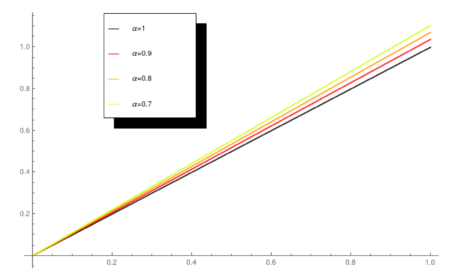
Using PLSM for several fractional values for $\alpha$, we obtain in the same manner:

• For $\alpha =0.9$: ${\tilde{x}}_{0.9}\left(t\right)=1.0378372034911354·t$,
• For $\alpha =0.8$: ${\tilde{x}}_{0.8}\left(t\right)=1.0711968661330562·t$,
• For $\alpha =0.7$: ${\tilde{x}}_{0.7}\left(t\right)=1.1045793185308062·t$.

Figure 1 presents the plots of these approximate solutions:

3.4. Application 4: Volterra Nonlinear Fractional Integro-Differential Equation

The next example consists of the Volterra equation ([15,16,20]):

$$D^{0.8}x\left(t\right)-\underset{0}{\overset{t}{\int }}(t-s)·x{\left(s\right)}^{2}ds-f\left(t\right)=0,$$

(16)

where $f\left(t\right)={\displaystyle \frac{25t^{6/5}}{3\mathsf{\Gamma }\left(\frac{1}{5}\right)}}+{\displaystyle \frac{t^6}{30}}-{\displaystyle \frac{t^5}{10}}+{\displaystyle \frac{t^4}{12}}+{\displaystyle \frac{5\sqrt[5]{t}}{\mathsf{\Gamma }\left(\frac{1}{5}\right)}}$, together with the condition $x\left(0\right)=0$.

The exact solution of the problem is $x_e\left(t\right)=t^2-t$.

Using PLSM with $\tilde{x}\left(t\right)=c_2·t^2+c_1·t+c_0$ we find from the condition that $c_0=0$ and the reminder (9) is

$$R(t,c_1,c_2)={\displaystyle \frac{5\sqrt[5]{t}(3c_1+5c_2-1)t+3)}{3\mathsf{\Gamma }\left(\frac{1}{5}\right)}}-{\displaystyle \frac{1}{60}}{t}^4\{5c_1^2+6c_1{c}_{2}t+2t[\left(c_2^2-1\right)t+3]-5\}.$$

Minimizing the corresponding functional $J(c_1,c_2)$ (too long to be included here) we get $c_1=-1$ and $c_2=1$ which means that we obtain in fact the exact solution $\tilde{x}=x_e=t^2-1$. Again we remark that the previous methods in [15] (Euler Wavelets Method), [16] (Lucas Wavelets Method) and [20] (Chebyshev Wavelets Method) were only able to find approximate solutions.

3.5. Application 5: Volterra Fractional Integro-Differential Equation

We consider the Volterra equation ([19,20,24]):

$$D^{\sqrt{3}}x\left(t\right)-\underset{0}{\overset{t}{\int }}x\left(s\right)cos(s-t)ds-f\left(t\right)=0,$$

(17)

where $f\left(t\right)={\displaystyle \frac{2\left(2+\sqrt{3}\right)t^{2-\sqrt{3}}}{\mathsf{\Gamma }\left(2-\sqrt{3}\right)}}+2t-2sin\left(t\right)$.

The problem consists of the Equation (17), together with the conditions

$$-x^{\prime }\left(0\right)-x^{\prime }\left(1\right)+x\left(0\right)+x\left(1\right)=-1,x^{\prime }\left(0\right)-3·x^{\prime }\left(1\right)+3·x\left(0\right)+4·x\left(1\right)=-2.$$

Using PLSM, we choose $\tilde{x}\left(t\right)=c_2·t^2+c_1·t+c_0$. By using the initial conditions, we find $c_0={\displaystyle \frac{4}{11}}·(c_2-1),c_1=-{\displaystyle \frac{3}{11}}·(c_2-1)$ and the corresponding reminder

$$R(t,c_2)={\displaystyle \frac{2\left(2+\sqrt{3}\right)c_2{t}^{2-\sqrt{3}}}{\mathsf{\Gamma }\left(2-\sqrt{3}\right)}}+{\displaystyle \frac{1}{11}}(-22c_{2}t+2(9c_2+2)sin\left(t\right)-3c_2-1)cos\left(t\right)+3c_2-3)-{\displaystyle \frac{2\left(2+\sqrt{3}\right)t^{2-\sqrt{3}}}{\mathsf{\Gamma }\left(2-\sqrt{3}\right)}}+2t-2sin\left(t\right),$$

and after minimizing the functional $J\left(c_2\right)$, we find the minimum as $c_2=1$. Thus, $\tilde{x}=t^2$, which is the exact solution of the problem while, again, the previous methods in [19] (Chebyshev Wavelets Method), Ref. [20] (also a Chebyshev Wavelets Method) and [24] (Newton–Kantorovitch Method) were only able to find approximate solutions.

3.6. Application 6: Volterra Nonlinear Fractional Integro-Differential Equation

We consider the problem consisting of the Volterra equation ([2,16]):

$$D^{\alpha }x\left(t\right)-\underset{0}{\overset{t}{\int }}st{e}^{-x{\left(s\right)}^2}ds-\frac{1}{2}{e}^{-t^2}t+\frac{t}{2}=1,0<\alpha \le 1,$$

(18)

together with the condition $x\left(0\right)=0$.

For $\alpha =1$ by using the same PLSM steps as above we obtain the exact solution of the problem $\tilde{x}\left(t\right)=x_e=t$.

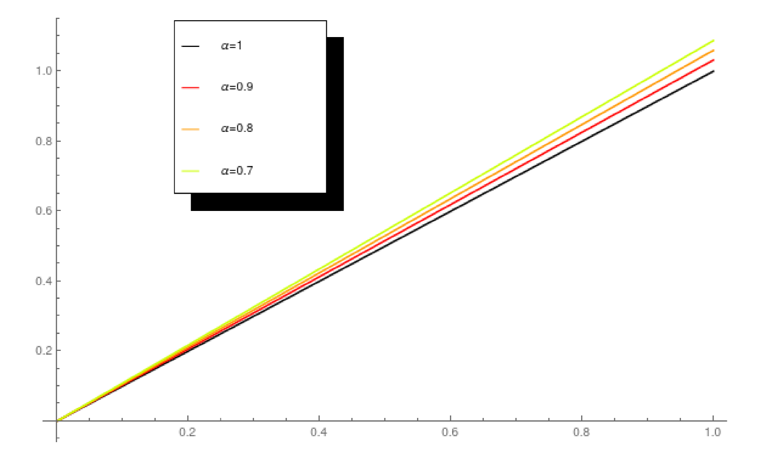
Using PLSM for several fractional values for $\alpha$, we obtain in the same manner:

• For $\alpha =0.9$: ${\tilde{x}}_{0.9}\left(t\right)=1.0320545396738823·t$,
• For $\alpha =0.8$: ${\tilde{x}}_{0.8}\left(t\right)=1.0599257897790655·t$,
• For $\alpha =0.7$: ${\tilde{x}}_{0.7}\left(t\right)=1.0877449515729398·t$.

Figure 2 presents the plots of these approximate solutions:

3.7. Application 7: Volterra Fractional Integro-Differential Equation

We consider the Volterra equation ([2,16]):

$$\begin{array}{c}{D}^{\alpha }x\left(t\right)+x\left(t\right)cos\left(t\right)-sin\left({\displaystyle \frac{t}{2}}\right)\underset{0}{\overset{t}{\int }}x\left(s\right)cos\left(2s\right)ds+f\left(t\right)=0,0<\alpha \le 1,\end{array}$$

(19)

where

$$f\left(t\right)={\displaystyle \frac{2}{9}}sin\left({\displaystyle \frac{t}{2}}\right)sin\left(3t\right)-{cos}^2\left(t\right)-tcost+{\displaystyle \frac{1}{2}}tsin\left({\displaystyle \frac{t}{2}}\right)cost-{\displaystyle \frac{1}{6}}tsin\left({\displaystyle \frac{t}{2}}\right)cos\left(3t\right)-tsintcost.$$

To this equation, we attach the conditions $x\left(0\right)=1,x^{\prime }\left(0\right)=0$.

The exact solution of this problem is only known in the case $\alpha =1$, when the exact solution is $x_e\left(t\right)=t·sin\left(t\right)+cos\left(t\right)$.

In this case, using PLSM, we compute the following approximate polynomial solutions:

• Approximate polynomial solution of 5th degree:
  $\tilde{x}\left(t\right)=0.018589569513826232·t^5-0.14360021800164882·t^4+0.008034207812100387·t^3$$+0.4987467983166054·t^2+1$,
• Approximate polynomial solution of 6th degree:
  $\tilde{x}\left(t\right)=0.005743110243275618·t^6+0.0020795756371049245·t^5-0.12645251284260617·t^4+0.00045575503910599835·t^3+0.49994729663945314·t^2+1$,
• Approximate polynomial solution of 7th degree:
  $\tilde{x}\left(t\right)=-0.0006386657345089364·t^7+0.007914893567372211·t^6-0.0007605371942713338·t^5-0.12468062617297578·t^4-0.00006729076308001347·t^3+0.5000055205534544·t^2+1$,
• Approximate polynomial solution of 8th degree:
  $\tilde{x}\left(t\right)=-0.00014575197807209506·t^8-0.00006753051750924·t^7+0.007018024380857246·t^6-0.00004334207390915834·t^5-0.12498593095838928·t^4-2.3296681712081657·{10}^{-6}·t^3+0.500000151553348·t^2+1$,
• Approximate polynomial solution of 9th degree:
  $\tilde{x}\left(t\right)=0.00001126919563446821·t^9-0.00019569241771572043·t^8+0.000023812835867415005·t^7+0.006929219156347782·t^6+5.8199183788354425·{10}^{-6}·t^5-0.1250012745238175·t^4+1.4253540456254932·{10}^{-7}·t^3+0.4999999939756038·t^2+1$.

Table 1. Comparison of the absolute errors of the approximate solutions for problem (19) corresponding to $\alpha =1$.

t	[16]	PLSM 5-th deg	PLSM 6-th deg.	PLSM 7-th deg.	PLSM 8-th deg.	PLSM 9-th deg
0	0	0	0	0	0	0
0.1	$4.30\times {10}^{-12}$	$6.17\times {10}^{-6}$	$1.96\times {10}^{-7}$	$1.31\times {10}^{-8}$	$2.26\times {10}^{-10}$	$1.55\times {10}^{-14}$
0.2	$7.45\times {10}^{-12}$	$1.01\times {10}^{-5}$	$1.97\times {10}^{-7}$	$4.50\times {10}^{-8}$	$1.84\times {10}^{-11}$	$1.81\times {10}^{-12}$
0.3	$1.68\times {10}^{-11}$	$6.40\times {10}^{-6}$	$1.42\times {10}^{-8}$	$2.02\times {10}^{-9}$	$6.05\times {10}^{-11}$	$7.92\times {10}^{-12}$
0.4	$3.16\times {10}^{-10}$	$4.62\times {10}^{-7}$	$3.91\times {10}^{-8}$	$6.83\times {10}^{-9}$	$2.33\times {10}^{-10}$	$1.95\times {10}^{-12}$
0.5	$2.04\times {10}^{-9}$	$1.55\times {10}^{-6}$	$9.68\times {10}^{-8}$	$1.23\times {10}^{-8}$	$6.77\times {10}^{-10}$	$6.80\times {10}^{-12}$
0.6	$8.49\times {10}^{-9}$	$1.92\times {10}^{-6}$	$2.16\times {10}^{-7}$	$3.84\times {10}^{-9}$	$7.80\times {10}^{-11}$	$6.93\times {10}^{-12}$
0.7	$2.55\times {10}^{-8}$	$6.96\times {10}^{-6}$	$1.31\times {10}^{-7}$	$3.39\times {10}^{-9}$	$1.19\times {10}^{-10}$	$4.47\times {10}^{-12}$
0.8	$5.64\times {10}^{-8}$	$7.33\times {10}^{-6}$	$4.23\times {10}^{-8}$	$4.85\times {10}^{-9}$	$1.69\times {10}^{-10}$	$8.00\times {10}^{-12}$
0.9	$8.09\times {10}^{-8}$	$1.49\times {10}^{-6}$	$3.20\times {10}^{-8}$	$8.41\times {10}^{-9}$	$5.78\times {10}^{-11}$	$6.86\times {10}^{-12}$
1	$2.29\times {10}^{-9}$	$2.93\times {10}^{-6}$	$6.59\times {10}^{-8}$	$3.57\times {10}^{-9}$	$6.21\times {10}^{-11}$	$3.32\times {10}^{-13}$

presents the absolute errors corresponding to these solutions. The errors corresponding to PLSM are smaller than the ones in [16] (Lucas Wavelets Method) and about the same as the ones in [2] (Homotopy Perturbation Method), where only the norms corresponding to the errors were presented.

Table 1 also clearly illustrates the convergence of the method, since the errors decrease as the degree increases.

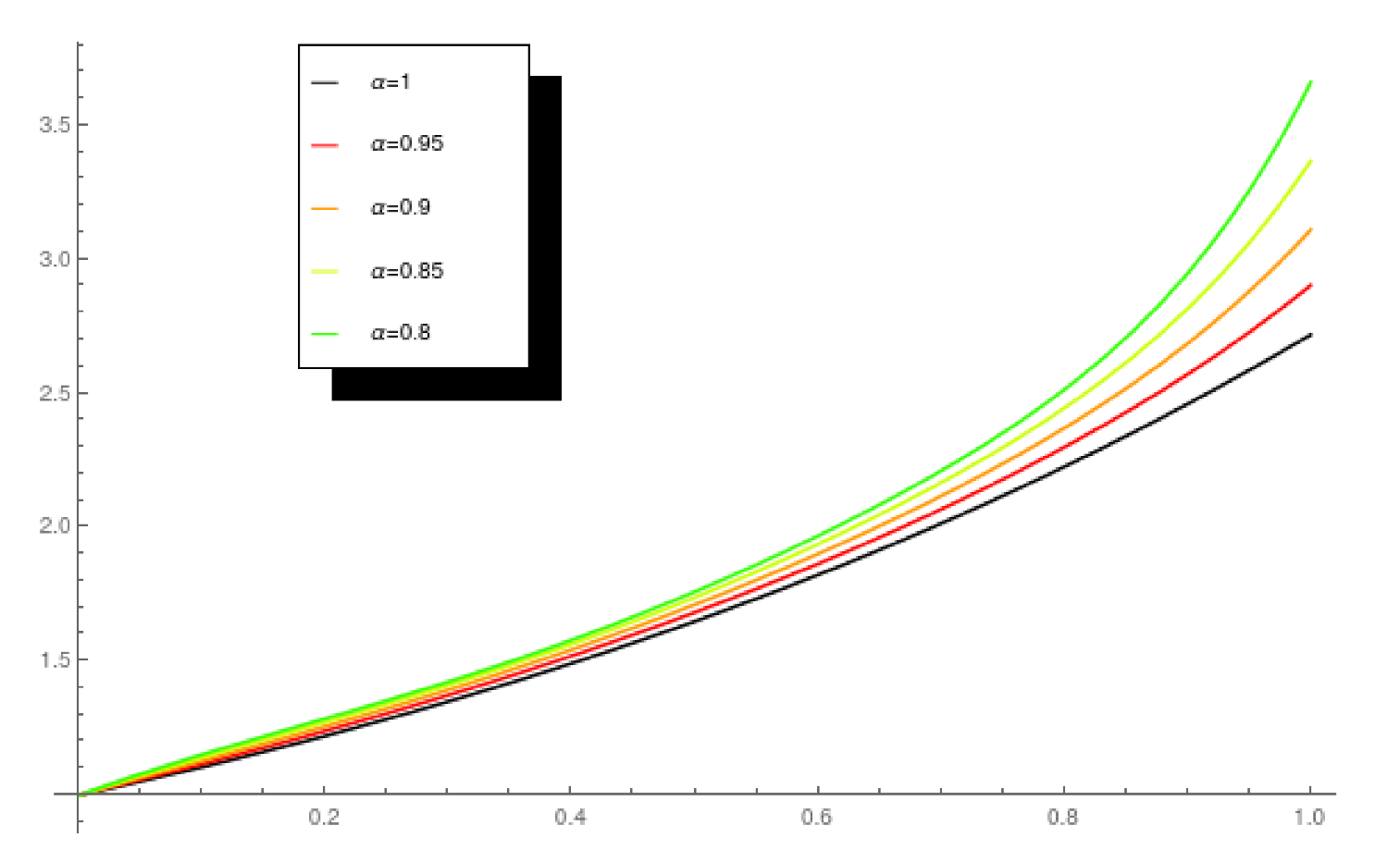
We also compute the following approximate solutions corresponding to fractional values for $\alpha$:

• For $\alpha =0.9$: ${\tilde{x}}_{0.9}\left(t\right)=-1.378568639242069·t^9+6.685078885808115·t^8-13.701094654510017·t^7+15.472065079508422·t^6-10.535788531855735·t^5+4.390956825059652·t^4-1.3038516398599118·t^3+0.7712852812834081·t^2+1$,
• For $\alpha =0.8$: ${\tilde{x}}_{0.8}\left(t\right)=-4.259445469061426·t^9+20.55460957565543·t^8-41.89105668604517·t^7+46.96639018648651·t^6-31.675110523819868·t^5+13.195321947793483·t^4-3.639243962350954·t^3+1.165260153885771{\dot{t}}^2+1$,
• For $\alpha =0.7$: ${\tilde{x}}_{0.7}\left(t\right)=-9.667413934605774·t^9+46.407467633601094·t^8-94.00740813159496·t^7+104.59349985560875·t^6-69.7865719594028·t^5+28.658004320777366·t^4-7.487972610113421·t^3+1.7220645113921877·t^2+1$.

Figure 3 presents the ninth degree polynomial approximate solutions of (19) for several fractional values of $\alpha$.

3.8. Application 8: Volterra–Fredholm Nonlinear Fractional Integro-Differential Equation

The next application is the Volterra–Fredholm equation ([25]):

$$D^{\sqrt{3}}x\left(t\right)-\underset{0}{\overset{1}{\int }}s{t}^{2}x{\left(s\right)}^{2}ds-\underset{0}{\overset{t}{\int }}(s+t)x{\left(s\right)}^{3}ds-f\left(t\right)=0,$$

(20)

where $f\left(t\right)={\displaystyle \frac{2\left(2+\sqrt{3}\right)t^{2-\sqrt{3}}}{\mathsf{\Gamma }\left(2-\sqrt{3}\right)}}-{\displaystyle \frac{15t^8}{56}}-{\displaystyle \frac{t^2}{6}}$,

together with the conditions $x^{\prime }\left(0\right)+x\left(0\right)=0,x^{\prime }\left(1\right)+x\left(1\right)=3$.

While in [25] approximate solutions computed by a Block-pulse Functions Method were presented, by using PLSM we are able to find the exact solution, $x_e\left(t\right)=t^2$.

3.9. Application 9: Volterra–Fredholm Nonlinear Fractional Integro-Differential Equation

We consider the problem consisting of the Volterra–Fredholm equation ([6,20]):

$$D^{2.2}x\left(t\right)-\frac{1}{3}\underset{0}{\overset{t}{\int }}(s+t)x{\left(s\right)}^{2}ds-\frac{1}{4}\underset{0}{\overset{1}{\int }}(t-s)x{\left(s\right)}^{3}ds-f\left(t\right)=0,$$

(21)

where $f\left(t\right)={\displaystyle \frac{15t^{4/5}}{2\mathsf{\Gamma }\left(\frac{4}{5}\right)}}-{\displaystyle \frac{5t^8}{56}}-{\displaystyle \frac{t}{40}}+{\displaystyle \frac{1}{44}}$,

together with the conditions $x\left(0\right)=0,x^{\prime }\left(0\right)=0,x^{\prime \prime }\left(0\right)=0$.

Again, while the methods in [6] (Legendre Wavelets Method) and [20] (Chebyshev Wavelets Method) are able to find good approximate solutions, by using PLSM we are able to find the exact solution of the problem, $x_e\left(t\right)=t^3$.

3.10. Application 10: Volterra–Fredholm Fractional Integro-Differential Equation

The next example is the Volterra–Fredholm equation ([6,14,20]):

$$D^{1.7}x\left(t\right)-\underset{0}{\overset{t}{\int }}(t-s)x\left(s\right)ds-\underset{0}{\overset{1}{\int }}(s+t)x\left(s\right)ds-f\left(t\right)=0,$$

(22)

where $f\left(t\right)={\displaystyle \frac{20t^{3/10}}{3\mathsf{\Gamma }\left(\frac{3}{10}\right)}}+{\displaystyle \frac{200t^{13/10}}{13\mathsf{\Gamma }\left(\frac{3}{10}\right)}}-{\displaystyle \frac{t^5}{20}}+{\displaystyle \frac{t^4}{12}}-{\displaystyle \frac{7t}{12}}-{\displaystyle \frac{9}{20}}$,

presented together with the conditions $x\left(0\right)=0,x^{\prime }\left(0\right)=0$.

Once again, while by using the methods in [6] (Legendre Wavelets Method), Ref. [14] (Genocchi Polynomials Method) and [20] (Chebyshev Wavelets Method) one is able to find good approximate solutions, by using PLSM we are able to find the exact solution of the problem, $x_e\left(t\right)=t^3+t^2$.

3.11. Application 11: Volterra-Fredholm Fractional Integro-Differential Equation

The 11th application consists of the Volterra–Fredholm equation ([6,14,20]):

$$D^{2.3}x\left(t\right)-{\displaystyle \frac{1}{4}}\underset{0}{\overset{t}{\int }}(t-s)x\left(s\right)ds-{\displaystyle \frac{1}{2}}\underset{0}{\overset{1}{\int }}stx\left(s\right)ds-f\left(t\right)=0,$$

(23)

where $f\left(t\right)=-{\displaystyle \frac{t^{11/2}}{99}}+{\displaystyle \frac{105\sqrt{\pi }{t}^{6/5}}{16\mathsf{\Gamma }\left(\frac{11}{5}\right)}}-{\displaystyle \frac{t}{11}}$,

together with the set of conditions $x\left(0\right)=0,x^{\prime }\left(0\right)=0,x^{\prime \prime }\left(0\right)=0$.

The exact solution is $x_e\left(t\right)=t^{\frac{7}{2}}$.

By using PLSM, we compute polynomial approximate solutions of several degrees, among which we present here the following:

• 7th degree approximate polynomial solution:
  $\tilde{x}\left(t\right)=-0.16324698892355705·t^7+0.6185882652367157·t^6-1.0271245965900326·t^5+1.3473031097371286·t^4+0.22490807225586334·t^3$,
• 10th degree approximate polynomial solution:
  $\tilde{x}\left(t\right)=1.021320674686219·t^{10}-4.917717536478034·t^9+10.184078575662898·t^8-11.911201753058227·t^7+8.757511916799231·t^6-4.409295003548161·t^5+2.1308709245644373·t^4+0.14462933332093625·t^3$,
• 13th degree approximate polynomial solution:
  $\tilde{x}\left(t\right)=-14.85841263752164·t^{13}+89.90598535471365·t^{12}-241.38875274938806·t^{11}+378.9435225695182·t^{10}-385.983259780314·t^9+267.89170150609334·t^8-129.8133521171707·t^7+44.627485832332916·t^6-11.32725213934628·t^5+2.8951478603715883·t^4+0.10703132594996229·t^3$.

Table 2. Comparison of the absolute errors of the approximate solutions for problem (23).

t	[6]	[14]	[20]	PLSM 7-th deg.	PLSM 10 deg.	PLSM 13 deg
0	0	0	0	0	0	0
$\frac{1}{8}$	$6.64\times {10}^{-6}$	$1.61\times {10}^{-4}$	$3.35\times {10}^{-6}$	$4.86\times {10}^{-5}$	$5.91\times {10}^{-6}$	$1.41\times {10}^{-6}$
$\frac{2}{8}$	$4.53\times {10}^{-5}$	$6.47\times {10}^{-4}$	$1.73\times {10}^{-5}$	$1.02\times {10}^{-4}$	$1.38\times {10}^{-5}$	$3.74\times {10}^{-6}$
$\frac{3}{8}$	$3.14\times {10}^{-5}$	$1.27\times {10}^{-3}$	$3.79\times {10}^{-5}$	$1.44\times {10}^{-4}$	$2.43\times {10}^{-5}$	$6.42\times {10}^{-6}$
$\frac{4}{8}$	$7.37\times {10}^{-5}$	$1.94\times {10}^{-3}$	$6.29\times {10}^{-5}$	$2.24\times {10}^{-4}$	$3.32\times {10}^{-5}$	$9.10\times {10}^{-6}$
$\frac{5}{8}$	$2.44\times {10}^{-4}$	$2.66\times {10}^{-3}$	$9.14\times {10}^{-5}$	$3.16\times {10}^{-4}$	$4.65\times {10}^{-5}$	$1.24\times {10}^{-5}$
$\frac{6}{8}$	$3.81\times {10}^{-4}$	$3.43\times {10}^{-3}$	$1.23\times {10}^{-4}$	$3.87\times {10}^{-4}$	$5.77\times {10}^{-5}$	$1.55\times {10}^{-5}$
$\frac{7}{8}$	$6.02\times {10}^{-4}$	$4.26\times {10}^{-3}$	$1.56\times {10}^{-4}$	$4.72\times {10}^{-4}$	$7.12\times {10}^{-5}$	$1.91\times {10}^{-5}$

presents the absolute errors corresponding to these solutions and to the most accurate included in [6] (Legendre Wavelets Method), [14] (Genocchi Polynomials Method) and [20] (Chebyshev Wavelets Method). Table 2 also illustrates again the convergence of the method, as the errors decrease as the degree increases (and this is true for all degrees, not only for the polynomials presented here).

3.12. Application 12: Volterra–Fredholm Fractional Nonlinear Integro-Differential Equation

The 12th application consists of the Volterra–Fredholm equation ([11,16,29])

$$D^{\alpha }x\left(t\right)+2tx\left(t\right)-\underset{0}{\overset{1}{\int }}(t-s)x\left(s\right)ds-\underset{0}{\overset{t}{\int }}(s+t)x^3\left(s\right)ds-f\left(t\right)=0,0<\alpha \le 1,$$

(24)

where $f\left(t\right)=e^t+2e^{t}t-{\displaystyle \frac{2}{3}}{e}^{3t}t-et+{\displaystyle \frac{4t}{3}}+{\displaystyle \frac{e^{3t}+8}{9}}$,

together with the initial condition $x\left(0\right)=1$.

The exact solution is only known for the case $\alpha =1$, namely $x_e\left(t\right)=e^t$.

By using PLSM, we compute polynomial approximate solutions of several degrees, among which we present here the following:

• 6th degree approximate polynomial solution:
  $\tilde{x}\left(t\right)=0.0023155227591934115516·t^6+0.0069500055653780543873·t^5+0.042632588272403311485·t^4+0.16633572610736494044·t^3+0.50005031966286137278·t^2+0.99999759249220231145·t+1$,
• 7th degree approximate polynomial solution:
  $\tilde{x}\left(t\right)=0.00033027387015192981120·t^7+0.0011564590016090762375·t^6+0.0085352350377548106611·t^5+0.041573019954592717180·t^4+0.16668920666965779451·t^3+0.49999755331735148173·t^2+1.0000000782522148130·t+1$,
• 8th degree approximate polynomial solution:
  $\tilde{x}\left(t\right)=0.000040762555962133136849·t^8+0.00016673821949108303496·t^7+0.0014211306083055067049·t^6+0.0083147094634950057743·t^5+0.041672857762811908105·t^4+0.16666552647371937470·t^3+0.50000010771881998446·t^2+0.99999999496802995030·t+1$,
• 9th degree approximate polynomial solution:
  $\tilde{x}\left(t\right)=0.000020115943649341869522·t^9-0.000047507659492612516580·t^8+0.00032607553769710332881·t^7+0.0012688813051080890275·t^6+0.0083971443102209661202·t^5+0.041647795052332766250·t^4+0.16666948320634820205·t^3+0.49999984023895502665·t^2+0.99999999936990945418·t+1$.

Table 3. Comparison of the absolute errors of the approximate solutions for problem (24) corresponding to $\alpha =1$.

t	[11]	[29]	[16]	PLSM 6-th	PLSM 7-th	PLSM 8-th	PLSM 9-th
0	0	0	0	0	0	0	0
$0.2$	$3.4\times {10}^{-6}$	$1.8\times {10}^{-9}$	$1.9\times {10}^{-10}$	$4.3\times {10}^{-8}$	$3.7\times {10}^{-10}$	$1.7\times {10}^{-10}$	$1.8\times {10}^{-11}$
$0.4$	$5.9\times {10}^{-6}$	$1.3\times {10}^{-9}$	$4.4\times {10}^{-10}$	$7.6\times {10}^{-8}$	$4.8\times {10}^{-10}$	$9.2\times {10}^{-11}$	$5.0\times {10}^{-10}$
$0.6$	$6.1\times {10}^{-5}$	$1.1\times {10}^{-9}$	$6.3\times {10}^{-10}$	$3.6\times {10}^{-8}$	$1.1\times {10}^{-9}$	$2.1\times {10}^{-10}$	$8.3\times {10}^{-13}$
$0.8$	$7.6\times {10}^{-6}$	$1.1\times {10}^{-9}$	$6.8\times {10}^{-10}$	$7.2\times {10}^{-8}$	$9.2\times {10}^{-10}$	$2.6\times {10}^{-10}$	$6.7\times {10}^{-10}$
1	$8.5\times {10}^{-6}$	$9.1\times {10}^{-8}$	$3.6\times {10}^{-9}$	$7.3\times {10}^{-8}$	$2.3\times {10}^{-9}$	$6.9\times {10}^{-10}$	$9.9\times {10}^{-10}$

presents the absolute errors corresponding to these solutions and to the most accurate ones presented in [11] (Legendre Collocation Method), [29] (Bernstein Collocation Method) and [16] (Lucas Wavelets Method), illustrating at the same time the convergence of the method.

For fractional values of $\alpha$, we compute by using PLSM the following approximate solutions, plotted in Figure 4:

• For $\alpha =0.95$: ${\tilde{x}}_{0.95}\left(t\right)=0.39845808132897475299·t^7-0.28741165181585350444·t^6-0.12316665161332894420·t^5-0.078261148763147219616·t^4+0.76308271973377805651·t^3+0.071987504424180859600·t^2+1.1578214235211880623·t+1$,
• For $\alpha =0.9$: ${\tilde{x}}_{0.9}\left(t\right)=0.98363393805529270592·t^7-0.56506104464872151695·t^6-0.69439156749868620292·t^5+0.054345021330277263964·t^4+1.4505259764032931501·t^3-0.43542713404518504383·t^2+1.3162092563240184272·t+1$,
• For $\alpha =0.85$: ${\tilde{x}}_{0.85}\left(t\right)=1.9831650062101352206·t^7-1.1690757595826590608·t^6-1.3604243441778751218·t^5-0.10508833350315760611·t^4+2.7217752503812776606·t^3-1.2051974129678996454·t^2+1.5021941130959725097·t+1$,
• For $\alpha =0.8$: ${\tilde{x}}_{0.8}\left(t\right)=3.6063786168531715004·t^7-2.2174306545610186303·t^6-2.7765099058142735992·t^5+0.47581205102930625758·t^4+3.9233948885557306991·t^3-2.0308610220243491314·t^2+1.6804917092233814789·t+1$.

3.13. Application 13: Fredholm Fractional Integro-Differential Equation

The 13th application consists of the Fredholm equation ([11,16,30,31]):

$$D^{\alpha }x\left(t\right)-x\left(t\right)-\underset{0}{\overset{1}{\int }}{e}^{ts}x\left(s\right)ds+{\displaystyle \frac{e^{t+1}-1}{t+1}}=0,0<\alpha \le 1,$$

(25)

together with the initial condition $x\left(0\right)=1$.

The exact solution is only known for the case $\alpha =1$, namely $x_e\left(t\right)=e^t$. For this case, approximate solutions were previously computed by using a hybrid Fourier and Block-pulse functions method in [30], by using a Taylor polynomials method in [31], by using a Legendre collocation method in [11] and by using a Lucas wavelets method in [16].

By using PLSM, we compute polynomial approximate solutions of several degrees, including the following:

• 10th degree approximate polynomial solution: $\tilde{x}\left(t\right)=0.0000004800784472141·t^{10}+0.000002161996158951·t^9+0.0000257498621699737t^8+0.000197465453627480·t^7+0.00138951228485587·t^6+0.00833305830220831·t^5+0.0416667475427406·t^4+0.166666651219604·t^3+0.500000001755479·t^2+0.99999999982747·t+1$,
• 11th degree approximate polynomial solution: $\tilde{x}\left(t\right)=0.0000000436149080372·t^{11}+0.0000002160475004709·t^{10}+0.0000286242547922675·t^9+0.0000246796289010594·t^8+0.000198506803553533·t^7+0.00138883867870146·t^6+0.00833335193207591·t^5+0.0416666619440129·t^4+0.166666667464487·t^3+0.499999999917657·t^2+1.00000000000730·t+1$,
• 12th degree approximate polynomial solution: $\tilde{x}\left(t\right)=0.0000000036328006861·t^{12}+0.0000000196306045202·t^{11}+0.0000002863400346429·t^{10}+0.0000027418895547599·t^9+0.000024813822806523754472t^8+0.00019840504717469716467·t^7+0.0013888923087574284089·t^6+0.0083333322444490813909·t^5+0.041666666909546321853·t^4+0.16666666662992156622·t^3+0.50000000000347109182·t^2+0.9999999999997201958·t+1$.

Since, unfortunately, the results in [11,16,30,31] were not presented in the same manner or for the same set of values of t, in

Table 4. Comparison of the order of the absolute errors of the approximate solutions for problem (25) corresponding to $\alpha =1$.

[30]	[31]	[11]	[16]	PLSM 10-th	PLSM 11-th	PLSM 12-th
${10}^{-5}$	${10}^{-5}$	${10}^{-13}$	${10}^{-11}$	${10}^{-11}$	${10}^{-12}$	${10}^{-14}$

we present the order of the absolute errors corresponding to the most accurate approximations in these studies, together with the ones corresponding to the above approximate solutions computed by PLSM.

3.14. Application 14: Volterra High Order Nonlinear Fractional Integro-Differential Equation

The last application consists of the Volterra equation ([12,32,33]):

$$D^{\alpha }x\left(t\right)-1-\underset{0}{\overset{t}{\int }}{e}^{-s}{x}^2\left(s\right)ds=0,3<\alpha \le 4,$$

(26)

together with the boundary conditions $x\left(0\right)=1,x^{\prime \prime }\left(0\right)=1,x\left(1\right)=e,x^{\prime \prime }\left(1\right)=e$.

The exact solution known for the case $\alpha =4$ is $x_e\left(t\right)=e^t$ and approximate solutions in this case were previously computed by using the Adomian Decomposition Method in [12,32] and by using a CAS wavelets method in [33].

Among the polynomial approximate solutions computed by PLSM, we present:

• 6th degree approximate polynomial solution: $\tilde{x}\left(t\right)=0.002331047548255614389301552·t^6+0.007092789669703467145868321·t^5+0.04220798182765420646574031·t^4+0.1666664711142428305291651·t^3+0.5·t^2+0.99998353829918911683021216·t+1$,
• 7th degree approximate polynomial solution: $\tilde{x}\left(t\right)=0.0003317112751896279453899316·t^7+0.001170104816778469606816276·t^6+0.008485813064556347688193642·t^5+0.04162754541042999949590209·t^4+0.1666666673635733042891207·t^3+0.5·t^2+0.99999998652851748633486485·t+1$,
• 8th degree approximate polynomial solution: $\tilde{x}\left(t\right)=0.0000413625999468556050467252862352·t^8+0.000166260864693921086479659828095·t^7+0.00141825314334498986588556513346·t^6+0.00832044570322558260431576354844·t^5+0.0416688373177704165165092038074·t^4+0.166666668394461714930755411980·t^3+0.5·t^2+1.0000000004356017547512951417687·t+1$.

Again, the results in [12,32,33] were not presented as errors for a given set of values of t. The results obtained by the Adomian Decomposition Method were presented in [32] as a plot of the error function corresponding to the approximation, while in [33], the results obtained by the CAS wavelets method were presented by means of the approximate norm-2 (${\parallel er\left(t\right)\parallel }_2$) of the error functions corresponding to the approximations.

Computing the corresponding norm-2 for our approximations by PLSM, in

Table 5. Comparison of the order of the absolute errors of the approximate solutions for problem (26) corresponding to $\alpha =4$.

[12,32]	[33]	PLSM 6-th	PLSM 7-th	PLSM 8-th
$4\times {10}^{-5}$	$2\times {10}^{-8}$	$2\times {10}^{-6}$	$9\times {10}^{-8}$	$1\times {10}^{-9}$

we present these results together with those corresponding to the most accurate approximations in the previous studies.

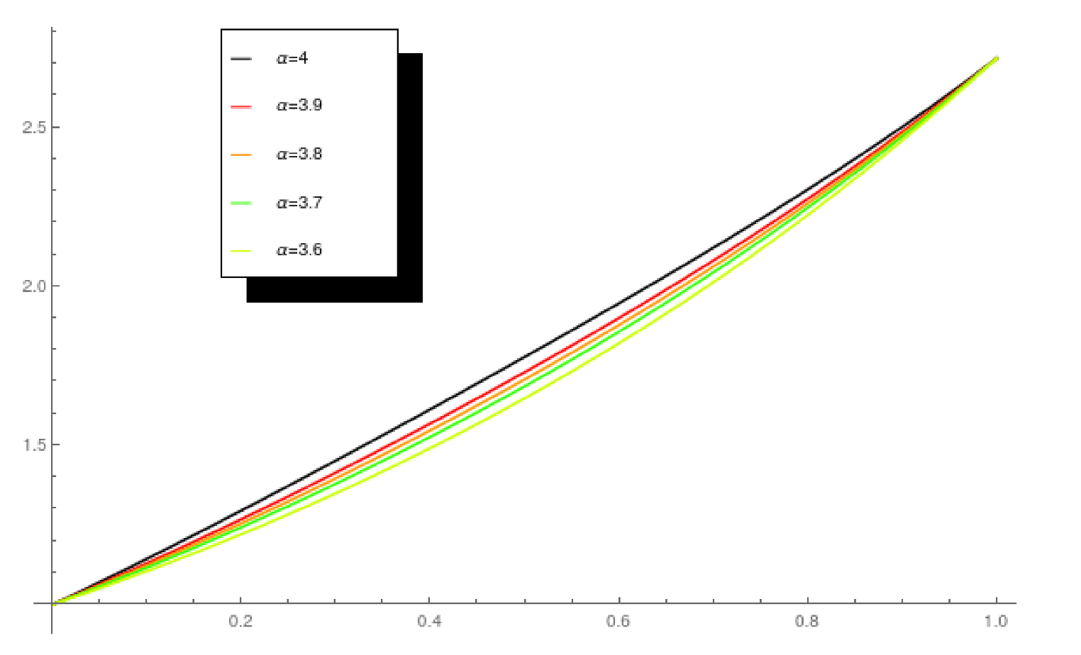
For fractional values of $\alpha$ we also computed by using PLSM several approximate solutions, plotted in Figure 5:

4. Conclusions

We presented the Polynomial Least Squares Method as a straightforward, efficient and accurate method to find approximate analytical solutions for a very general class of fractional nonlinear Volterra–Fredholm integro-differential equations.

The paper contains an extensive application list, including most of the usual test problems used for this type of equation and compare our results with previous results obtained by using other well-known methods. For the test problems where the exact solution is a polynomial one, PLSM is able to find the exact solution in a simple manner, while most of the other methods previously used were only able to compute approximate solutions. If the solution is not polynomial, PLSM is able to find approximate solutions, again in a very straightforward way, with errors usually smaller that the ones corresponding to the approximations computed by other methods.

Taking into the account the above considerations, the results of this paper recommend PLSM as a very useful tool in the study of fractional nonlinear integro-differential equations.

References

- Ghasemi, M.; Tavassoli, M.; Babolian, E. Application of He’s homotopy perturbation method to nonlinear integro-differential equations. Appl. Math. Comput. 2007, 188, 538–548. [Google Scholar] [CrossRef]
- Dehghan, M.; Shakeri, F. Solution of an integro-differential equation arising in oscillating magnetic fields using He’s homotopy perturbation method. Prog. Electromagn. Res. 2008, 78, 361–376. [Google Scholar] [CrossRef] [Green Version]
- Bhrawya, A.H.; Tohidic, E.; Soleymanic, F. A new Bernoulli matrix method for solving high-order linear and nonlinear Fredholm integro-differential equations with piecewise intervals. Appl. Math. Comput. 2012, 219, 482–497. [Google Scholar] [CrossRef]
- Keshavarz, E.; Ordokhani, Y.; Razzaghi, M. Numerical solution of nonlinear mixed Fredholm-Volterra integro-differential equations of fractional order by Bernoulli wavelets. Comput. Methods Differ. Equ. 2019, 7, 163–176. [Google Scholar]
- Rajagopal, N.; Balaji, S.; Seethalakshmi, R.; Balaji, V.S. A new numerical method for fractional order Volterra integro-differential equations. Ain Shams Eng. J. 2020, 11, 171–177. [Google Scholar] [CrossRef]
- Meng, Z.; Wang, L.; Li, H.; Zhang, W. Legendre wavelets method for solving fractionalintegro-differential equations. Int. J. Comput. Math. 2014, 92, 1275–1291. [Google Scholar] [CrossRef]
- Lotfi, M.; Alipanah, A. Legendre spectral element method for solving Volterra-integro differential equations. Results Appl. Math. 2020, 7, 1–11. [Google Scholar] [CrossRef]
- Al-Safi, M.G.S. An efficient numerical method for solving Volterra-Fredholm integro-differential equations of fractional order by using shifted Jacobi-spectral collocation method. Baghdad Sci. J. 2018, 15, 344–351. [Google Scholar]
- Arqub, O. A; Al-Smadi, M.; Shawagfeh, N. Solving Fredholm integro–differential equations using reproducing kernel Hilbert space method. Appl. Math. Comput. 2013, 219, 8938–8948. [Google Scholar]
- Alkan, S.; Hatipoglu, V.F. Approximate solutions of Volterra-Fredholm integro-differential equations of fractional order. Tbil. Math. J. 2017, 10, 1–13. [Google Scholar] [CrossRef]
- Rohaninasab, N.; Maleknejad, K.; Ezzati, R. Numerical solution of high-order Volterra–Fredholm integro-differential equations by using Legendre collocation method. Appl. Math. Comput. 2018, 328, 171–188. [Google Scholar] [CrossRef]
- Momani, S.; Noor, M.A. Numerical methods for fourth-order fractional integro-differential equations. Appl. Math. Comput. 2006, 182, 754–760. [Google Scholar] [CrossRef]
- Farhood, J.K. The solution of nonlinear fractional integro-differential equations by using shifted Chebyshev polynomials method and Adomian decomposition method. Int. J. Educ. Res. 2015, 5, 37–50. [Google Scholar]
- Loh, J.R.; Phang, C.; Isah, A. New operational matrix via Genocchi polynomials for solving Fredholm-Volterra fractional integro-differential equations. Adv. Math. Phys. 2017, 2017, 3821870. [Google Scholar] [CrossRef]
- Wang, Y.; Zhu, L. Solving nonlinear Volterra integro-differential equations of fractional order by using Euler wavelet method. Adv. Differ. Equ. 2017, 2017, 27. [Google Scholar] [CrossRef] [Green Version]
- Dehestani, H.; Ordokhani, Y.; Razzaghi, M. Combination of Lucas wavelets with Legendre–Gauss quadrature for fractional Fredholm-Volterra integro-differential equations. J. Comput. Appl. Math. 2021, 382, 1–18. [Google Scholar] [CrossRef]
- Dehghan, M.; Salehi, R. The numerical solution of the non-linear integro-differential equations based on the meshless method. J. Comput. Appl. Math. 2012, 236, 2367–2377. [Google Scholar] [CrossRef] [Green Version]
- Zhu, L.; Fan, Q. Numerical solution of nonlinear fractional-order Volterra integro-differential equations by SCW. Commun. Nonlinear Sci. Numer. Simul. 2013, 18, 1203–1213. [Google Scholar] [CrossRef]
- Mohyud-Din, S.T.; Khan, H.; Arif, M.; Rafiq, M. Chebyshev wavelet method to nonlinear fractional Volterra–Fredholm integro-differential equations with mixed boundary conditions. Adv. Mech. Eng. 2017, 9, 1–8. [Google Scholar] [CrossRef] [Green Version]
- Zhou, F.; Xu, X. Numerical solution of fractional Volterra-Fredholm integro-differential equations with mixed boundary conditions via Chebyshev wavelet method. Int. J. Comput. Math. 2018, 96, 436–456. [Google Scholar] [CrossRef]
- Parand, K.; Nikarya, M. Application of Bessel functions for solving differential and integro-differential equations of the fractional order. Appl. Math. Model. 2014, 38, 4137–4147. [Google Scholar] [CrossRef]
- Ordokhani, Y.; Dehestani, H. Numerical solution of linear Fredholm-Volterra integro-differential equations of fractional order. World J. Model. Simul. 2016, 12, 204–216. [Google Scholar]
- Ordokhani, Y.; Rahimi, N. Numerical solution of fractional Volterra integro-differential equations via the rationalized Haar functions. J. Sci. Kharazmi Univ. 2014, 14, 211–224. [Google Scholar]
- Susahab, D.N.; Jahanshahi, M. Numerical solution of nonlinear fractional Volterra-Fredholm integro-differential equations with mixed boundary conditions. Int. J. Ind. Math. 2015, 7, 63–69. [Google Scholar]
- Ali, M.R.; Hadhoud, A.R.; Srivastava, H.M. Solution of fractional Volterra–Fredholm integro-differential equations under mixed boundary conditions by using the HOBW method. Adv. Differ. Equ. 2019, 2019, 115. [Google Scholar] [CrossRef] [Green Version]
- Saadatmandi, A.; Akhlaghi, S. Using hybrid of Block-Pulse functions and Bernoulli polynomials to solve fractional Fredholm-Volterra integro-differential equations. Sains Malays. 2020, 49, 953–962. [Google Scholar] [CrossRef]
- Sabermahani, S.; Ordokhani, Y. A new operational matrix of Müntz-Legendre polynomials and Petrov-Galerkin method for solving fractional Volterra-Fredholm integro-differential equations. Comput. Methods Differ. Equ. 2020, 8, 408–423. [Google Scholar]
- Salman, N.K.; Mustafa, M.M. Numerical solution of fractional Volterra-Fredholm integro-differential equation using Lagrange polynomials. Baghdad Sci. J. 2020, 17, 1234–1240. [Google Scholar] [CrossRef]
- Yuzbasi, S. A collocation method based on Bernstein polynomials to solve nonlinear Fredholm-Volterra integro-differential equations. Appl. Math. Comput. 2016, 273, 142–154. [Google Scholar]
- Asady, B.; Kajani, M.T.; Vencheh, A.H.; Heydari, A. Direct method for solving integro-differential equations using hybrid Fourier and block-pulse functions. Int. J. Comput. Math. 2005, 82, 889–895. [Google Scholar] [CrossRef]
- Kurt, N.; Sezer, M. Polynomial solution of high-order linear Fredholm integro-differential equations with constant coefficients. J. Frankl. Inst. 2008, 345, 839–850. [Google Scholar] [CrossRef]
- Hashim, I. Adomian decomposition method for solving BVPs for fourth-order integro-differential equations. J. Comput. Appl. Math. 2005, 193, 658–664. [Google Scholar] [CrossRef] [Green Version]
- Saeedi, H.; Moghadam, M.M. Numerical solution of nonlinear Volterra integro-differential equations of arbitrary order by CAS wavelets. Commun. Nonlinear Sci. Numer. Simul. 2011, 16, 1216–1226. [Google Scholar] [CrossRef]
Figure 1.
Approximate solutions of (15) for several values of .
Figure 2.
Approximate solutions of (18) for several values of .
Figure 3.
Approximate solutions of (19) for several values of .
Figure 4.
Approximate solutions of (24) for several values of .
Figure 5.
Approximate solutions of (26) for several values of .