
A Bi-Level Programming Approach to the Location-Routing Problem with Cargo Splitting under Low-Carbon Policies

1
School of Economics & Management, Southeast University, Nanjing 211189, China
2
School of Maritime Economics and Management, Dalian Maritime University, Dalian 116026, China
*
Author to whom correspondence should be addressed.
Mathematics 2021, 9(18), 2325; https://0-doi-org.brum.beds.ac.uk/10.3390/math9182325
Submission received: 19 August 2021
/
Revised: 13 September 2021
/
Accepted: 16 September 2021
/
Published: 19 September 2021
(This article belongs to the Section Dynamical Systems)
Abstract
:To identify the impact of low-carbon policies on the location-routing problem (LRP) with cargo splitting (LRPCS), this paper first constructs the bi-level programming model of LRPCS. On this basis, the bi-level programming models of LRPCS under four low-carbon policies are constructed, respectively. The upper-level model takes the engineering construction department as the decision-maker to decide on the distribution center’s location. The lower-level model takes the logistics and distribution department as the decision-maker to make decisions on the vehicle distribution route’s scheme. Secondly, the hybrid algorithm of Ant Colony Optimization and Tabu Search (ACO-TS) is designed, and an example is introduced to verify the model’s and algorithm’s effectiveness. Finally, multiple sets of experiments are designed to explore the impact of various low-carbon policies on the decision-making of the LRPCS. The experimental results show that the influence of the carbon tax policy is the greatest, the carbon trading and carbon offset policy have a certain impact on the decision-making of the LRPCS, and the influence of the emission cap policy is the least. Based on this, we provide the relevant low-carbon policies advice and management implications.
1. Introduction
With the world population increasing and the scale of trade expanding rapidly, global warming and environmental pollution are becoming more and more serious, and extreme weather often occurs. Previous studies have shown that greenhouse gas emissions will seriously affect the ecological environment [1]. According to a report from the Washington Post [2], global carbon emissions were basically flat from 2014 to 2016, but global carbon emissions have steadily increased from 2017 to 2019. In 2020, global carbon dioxide emissions ushered in the largest absolute decline in the world’s history, about 7% lower than in 2019, or about 2.4 billion tons, equivalent to all of India’s carbon dioxide emissions in a normal year. However, the sharp drop in carbon emissions in 2020 is not due to the effectiveness of global emission reduction measures, but due to the COVID-19 pandemic, which has severely restricted the lives of residents and the production and operation of enterprises around the world. It can be seen that global carbon emissions have not been well-controlled. China is the largest emitter in the world, accounting for about 26% of global carbon emissions. However, as China is in a historical stage of rapid development and improving people’s livelihoods, the road of peaking carbon dioxide emissions and carbon neutrality has a long way to go. Globally, China’s road traffic carbon emissions accounted for 25% of the world’s total road traffic carbon emissions in 2020; in China, the transportation industry is the third-largest carbon emission department among all industries, and because China’s transportation is still in the stage of rapid development, its total emissions will continue to grow. The logistics industry has gradually become a major energy consumer and carbon emitter due to its rapid development. Therefore, research on the logistics industry’s carbon emission control strategy is of great significance to the realization of green logistics.
From the logistics operation system’s point of view, the distribution center’s daily operations and the distribution processes generate the main sources of carbon emissions, especially those generated by the distribution vehicles in the distribution process. Therefore, it is necessary to study vehicle routing optimization from the perspective of reducing carbon emissions. However, the distribution center’s location decision will have a restrictive effect on vehicle routing optimization, so they should be studied as a whole, namely, the location-routing problem (LRP). The LPR is not only a decision on the operation of logistics enterprises but also a decision on the strategic and tactical level. First, the distribution center’s location decision is a strategic and tactical decision, the location result will directly affect the distribution route choice of distribution vehicles, and the distribution center’s daily operations will produce corresponding carbon emissions. Secondly, among the logistics industry’s energy-conservation and emission-reduction measures, distribution vehicles, as the main source of carbon emissions, are the key areas of energy conservation and emission reduction. In addition to the introduction of new energy technologies, reasonable vehicle allocation and scheduling strategies are also crucial measures to reduce carbon emissions in the distribution process. In the LRP’s common research results, only one vehicle is generally allowed to provide services to customers; that is, cargo cannot split distribution. The existing scientific research results show that reasonably splitting customer demand for distribution can effectively reduce the no-load rate and distribution cost of distribution vehicles and bring more profit space to enterprises [3,4,5]. The LRP is a typical hierarchical decision-making problem, which requires the participation of multi-level decision-making, and the bi-level programming model has the advantage of collaborative optimization of different levels of problems. The location problem (LP) and vehicle-routing problem (VRP) can be jointly optimized by using the bi-level programming model, which reflects the logistics system’s hierarchy and integrity.
With the implementation of many energy-conservation and emission-reduction policies and the establishment of China’s carbon emissions trading market, low-carbon policies are bound to bring about various levels of decision-making impacts on various industries. The logistics industry will also face the challenges brought by the transition from a relatively broad low-carbon background to a further specific low-carbon policies background. Logistics enterprises’ distribution center locations, distribution vehicle routing, and other decisions will inevitably need to change from the traditional, simple low-emission orientation to the specific low-carbon policies guidance.
Considering this, it is necessary to take specific low-carbon policies (such as emission cap, carbon tax, carbon trading, and carbon offset, etc.) as the decision-making background, from the perspective of the joint participation of multi-level decision-makers, and use the bi-level programming model to study the LRP with cargo splitting (LRPCS).
The remainder of this paper is organized as follows. Section 2 reviews the related research. A general description of the research problem is provided in Section 3. Section 4 describes an Ant Colony Optimization and Tabu Search (ACO-TS) algorithm to solve the problem in this paper. Section 5 introduces an example to verify the effectiveness of the model and algorithm proposed in this paper, and several groups of experiments are designed to explore the impact of low-carbon policies on the LRPCS. Finally, the conclusions are presented in Section 6.
2. Literature Review
To study the LRPCS under the background of low-carbon policies, the existing research is reviewed from the following two aspects, which lays a good foundation for this paper: (1) The core problem that this paper tries to solve is the LRP. The research status of the LRP (both domestic and overseas) is investigated, and the commonly used models and solving algorithms for the LRP are reviewed to sort out the LRP considering carbon emissions and low-carbon policies. (2) The bi-level programming model has the advantage of hierarchical decision-making, which is suitable for solving the LRP. Therefore, the application status of bi-level programming in the LRP is summarized.
2.1. LRP
The study of modern LP can be traced back to 1909 [6]. In 1964, Hakimi proposed the landmark p-median problem and p-center problem on the network, which stimulated the theoretical study of the LP, and the number of studies increased sharply [7]. At present, there have been a large number of achievements in the research on LP of the logistics centers in the area of transport. Macioszek [8] presented the issues of logistics centers in terms of legal requirements for the functioning of logistics centers, rules, and methods of locating such facilities in the area of the transport network, which were supplemented by an analysis of the functioning of logistics centers in Poland in 2008–2018. Furthermore, some scholars combine green logistics with the LP. Urzúa-Morales et al. [9] used the methodology city logistics and last-mile to design the urban logistic system, and the physical location selection of the Cross-Docking was performed through an optimization model of maximum coverage. This design minimized the environmental impact of atmospheric pollution. Xu et al. [10] studied the LP of a green logistics park and built a single-objective decision model based on the comprehensive cost. Chang et al. [11] formulated a double objective function optimization model of reverse logistics facility location considering the balance between the functional objectives of the carbon emissions and the benefits, and proposed a hybrid multi-objective optimization algorithm that combines a gravitation algorithm and a particle swarm optimization algorithm.
In the 1970s, Cooper first proposed the LRP, combining LP with VRP, and many scholars have researched the model and its solving algorithm. In researching the LRP model, Li et al. [12,13,14,15,16] used a multi-objective model, Tokgoz et al. [17] established a mixed-integer non-linear programming problem to research the manifold LRP and provided the corresponding heuristic algorithm solution, and Tirkolaee et al. [18] established a new mixed-integer linear programming model, which aims to reduce the total travel time and minimize the risk of infection, and constructed a sustainable multi-travel time window LRP for medical waste management during the COVID-19 pandemic.
In researching the LRP algorithms, Mousavi et al. [19,20,21] designed a two-stage algorithm to solve the LRP, divided into LP and VRP, which cannot reflect the LRP’s integrity. The efficiency and quality of the optimal solution improve when the LRP is solved as a whole. Rybickova et al. [22] adopted a genetic algorithm to solve the continuous LRP. Zhang et al. [23] adopted an improved particle swarm optimization algorithm to solve the dynamic multi-objective LRP in the emergency response process of major oil spill accidents at sea. Sun [24] solved the capacitated hub LRP at the same time based on an endosymbiotic evolutionary algorithm. In addition, some scholars used hybrid algorithms to solve LRPs, such as Yu et al. [25], who designed a hybrid genetic algorithm to solve LRP with capacity constraints. Derbel et al. [26] used a hybrid algorithm including an iterative local search and genetic algorithm to deal with an LRP with multiple capacitated depots and one incapacitated vehicle per depot, making location and routing decisions efficient at the same time.
Given the vigorously developing green and low-carbon economies, the future development trend of the logistics industry with high energy consumption and large carbon emissions is to develop green logistics. The LRP plays a decisive role in the whole logistics system as a strategic logistics planning activity. A wealth of research has been achieved concerning the LRP of carbon emissions (see Table 1).
Through the review of the above literature, it can be found that most of the literature focuses on LRP research regarding how to reduce costs and carbon emissions. However, the low-carbon policies will not only reduce emissions by controlling the carbon emissions or generating carbon emission costs in the production and operation of logistics enterprises, but will also impact the economic decision-making of logistics enterprises. The location-routing decision of logistics enterprises changes accordingly under different carbon emission control policies. Therefore, it is necessary to further explore the impact of low-carbon policies on location-routing decision-making based on research on the LRP of reducing carbon emissions. Wang et al. [38] established a green low-carbon location-routing model of cold chain logistics, including carbon emission costs, and analyzed the impact of a carbon tax policy on the cold chain logistics network. Micheli et al. [39] studied the inventory routing problem under low-carbon policies, considering the uncertainty of customer demand and heterogeneous fleet, and discussed the impact of different carbon policies on the economy and environment. Liao et al. [40] constructed the electric vehicle routing model and traditional fuel vehicle routing model to explore the impact of electric vehicles on the cost and environment of logistics enterprises under the carbon trading policy. Zhou et al. [41] studied the robust optimization of multi-capacity LRP in the distribution network design under the carbon trading strategy.
LRP research has been relatively rich, and many scholars have researched the LRP considering carbon emissions, but there is a relative lack of research on the LRP in the context of specific carbon policies. However, in similar decision-making issues, the study of considering low-carbon policies has become very popular in recent years, including a large number of tactical decision-making problems, which shows that the implementation of low-carbon policies will have a substantial impact on corporate decision-making from the macro- to the micro-levels.
2.2. Application of Bi-Level Programming in the LRP
In the existing research on LRPs, most established multi-objective models and designed algorithms to solve them without considering the participation of multi-agents in decision-making. However, in the real world, the decision-making of each department is influenced by its superior, and at the same time, it also affects the decision-making of the subordinate department. The use of the single-level programming method will separate the interrelated objects, and is unable to conduct comprehensive analyses and treatments. Experts and scholars introduce bi-level programming into their studies of location and routing optimization because bi-level programming allows the use of the hierarchical decision-making planning method. The bi-level programming model embodies the idea of collaborative optimization of problems at different levels. The lower model’s decision must be made under the upper model’s decision, and the upper-level decision-maker must also adjust the decision in time according to the lower model’s results, and finally find the optimal solution that meets the upper and lower levels. The logistics system has a very distinct hierarchy, so it is more appropriate to analyze it with a bi-level model.
Xu et al. [42] proposed a bi-level model for a 72 h post-earthquake emergency logistics LRP under a random fuzzy environment. Nadizadeh et al. [43] used a bi-level programming model to study the arc interdiction LRP and proposed an efficient memetic algorithm based on a dynamic local search. Xu et al. [44] studied the multi-depot LRP considering a no-load backhaul in a collaborative logistics network based on a bi-level programming model. Parvasi et al. [45] established a bi-level model to study the efficient transportation system considering the response of students and designed appropriate bus stops and bus routes. Li et al. [46,47] used bi-level programming to study the location strategy of charging infrastructure and designed a two-stage heuristic algorithm to solve the problem. To ensure coordination and consider the interests of bus companies and passengers simultaneously, Cheng et al. [48] adopted the bi-level programming approach to solve the problem of optimal bus stop locations. Jiang et al. [49] used a bi-level programming model to study the design of a regional multimodal logistics network considering demand uncertainty and reducing carbon emissions and designed an adjustable robust optimization method to solve the problem. Li et al. [50] used bi-level programming to study the post-disaster road network repair scheduling and disaster relief logistics problems and designed a genetic algorithm to solve the model. Iliopoulou et al. [51] studied the joint traffic network design and toll infrastructure LP based on the bi-level programming model and designed a multi-objective particle swarm optimization algorithm to solve the problem.
Some scholars have studied the LRP based on the bi-level programming model, but the optimization goal of the research is generally to minimize the cost of the logistics system, with less consideration of carbon emissions; in particular, with the gradual implementation of low-carbon policies, decision-makers must consider the limitations of low-carbon policies when formulating location-routing strategies.
3. Problem Description and Model Formulation
3.1. Problem Description
It is assumed that a logistics enterprise must provide cargo distribution services for several customers in a certain area, in which the number, geographical location, and demand of customers are known. In several existing candidate distribution centers, the engineering construction department must select the appropriate distribution center among the candidate distribution centers and make a distribution center location decision. According to the distribution center’s location results, the logistics distribution department will decide on the route selection of distribution vehicles, arrange for distribution vehicles to assemble cargo from the selected distribution center, and distribute the cargo to each customer one-by-one according to the preset route. Different vehicles can access each customer, which splits the cargo’s distribution. When all the cargo is distributed, the distribution vehicle returns to the original distribution center.
The upper decision-maker’s engineering construction department formulates the distribution center’s location strategy to minimize the distribution center’s construction and operation costs and the distribution center’s carbon emissions related to the distribution center’s capacity, whereas the logistics department of the lower decision-maker mainly considers the dispatch costs, energy consumption costs, and carbon emissions in the distribution process to formulate the distribution route scheme. On this basis, with reference to [38,39,40,41], considering the background of specific carbon emission policies (emission cap, carbon tax, carbon trading, and carbon offset), the upper-level decision-makers mainly aim to minimize the distribution center’s construction, operation, and carbon emission costs generated by the distribution center, whereas the lower-level decision-makers mainly consider the dispatch, energy consumption, and carbon emissions costs generated in the distribution process, trying to find the optimal location and distribution route schemes to meet the cost and carbon emission requirements. A schematic diagram of the problem is shown in Figure 1.
The decision-making objectives of the two departments are inconsistent, and they each control some decision variables. Further, the engineering construction department’s location strategy will greatly affect the formulation of the logistics distribution department’s vehicle routing scheme. On the other hand, the logistics distribution department’s vehicle routing scheme will impact the distribution center’s selection strategy. The two decision-making behaviors influence each other but they cannot control each other.
This paper makes the following assumptions:
- The locations of the candidate distribution centers and customers are known, and the round-trip distance between the two points is the same.
- The customer demand is known, which is less than the distribution vehicle’s maximum loading capacity, and there is no limit on the distribution time.
- The capacities of the candidate distribution centers are known.
- All customers are allowed to split distribution.
- All cargo can be split and mixed.
- The distribution center has a certain number of distribution vehicles, and each distribution vehicle belongs to only one distribution center. There is no case in which multiple distribution centers dispatch the same vehicle at the same time.
- The distribution vehicles’ maximum driving distances are not considered.
- The carbon emissions generated by the distribution center are only related to capacity.
- The carbon emissions in the distribution process are only related to road conditions, vehicle types, vehicle load, driving distance, and speed.
- The carbon emission caps of the low-carbon policies are aimed at the carbon emissions generated in the whole LRP.
- The impact of low-carbon policies on location and vehicle routing schemes is proportional to their respective carbon emissions.
Among the assumptions mentioned above, items 1–3, 6, and 7 are common general assumptions in ordinary LRP research, whereas items 4 and 5 are unique to LRPCS. Items 8–11 are necessary assumptions to study LRPCS under the background of specific low-carbon policies.
The abbreviations, sets, parameters, and decision variables used in this paper are summarized in Table 2.
3.1.1. Measurement and Mathematical Description of Carbon Emissions
The carbon emissions in the model come from the carbon emissions generated by the distribution center’s operations and distribution vehicles during the distribution process. The specific measurements and mathematical descriptions are as follows:
- 1.
- Carbon emissions from distribution centers
In the LRP, the carbon emissions generated by the distribution center are related to the distribution center’s scale; then, the distribution center’s carbon emissions are as shown in Equation (1):
- 2.
- Carbon emissions of distribution vehicles
Fossil fuel-powered vehicles are bound to produce carbon emissions during operation. In the LRP, the carbon emissions generated by the distribution process mainly come from distribution vehicles, and the carbon emissions generated by distribution vehicles are related to many factors, such as vehicle type, vehicle load, driving speed, driving distance, fuel type, road conditions, traffic conditions, and so on. This paper introduces the measurement method of carbon emissions under land transportation to facilitate the problem’s calculation [52]. In a certain distribution process, the distribution vehicle drives from the customer point to the customer point , and the distribution vehicle’s carbon emission is in the distance arc . This emission is related to the fuel consumption and greenhouse gas emission coefficient generated by the distribution vehicle, and has the following relationship:
among them, is the greenhouse gas emission coefficient, which represents the carbon emission per unit of fuel. It is related to the vehicle type and fuel type used. It is generally set as a constant in the given logistics and distribution process, with reference to the European carbon emission calculation standard, = 2.32 kg/L.
The calculation of fuel consumption, , on the arc is mostly related to distance or load [52]. As a result, the calculation of the distribution vehicles’ fuel consumption does not align with reality. Therefore, this paper will comprehensively consider the influence of vehicle transportation distance, vehicle load, speed, vehicle type, and road condition on vehicle fuel consumption, and adopt the following calculation equation [53]:
among them, is the road condition coefficient of arc (related to road slope, resistance, etc.), and is the vehicle type coefficient (related to vehicle horsepower, windward area, etc.). According to [53], generally, , is related to the vehicle type and has a wide range of changes, and this paper will only consider one type of vehicle, assuming .
3.1.2. Cost Function Analysis and Mathematical Description
The cost function of the LRP’s bi-level programming model is mainly related to the distribution center’s construction and operation costs, the distribution vehicle’s energy consumption and dispatch costs in the distribution process, and the carbon emission costs under the specific low-carbon policies. Among them, the carbon emissions cost is related to the provisions of low-carbon policies, which will be described in the construction of bi-level programming models under specific low-carbon policies. Specific measurements and mathematical descriptions of other costs are as follows:
- 1.
- The distribution center’s construction and operation costs
Among the distribution center’s construction and operation costs, the construction costs mainly include the cost of land requisition, the lease and purchase of site and equipment, and so on. Operation costs mainly include employee wages, equipment maintenance depreciation costs, water and electricity consumption costs, and so on.
The distribution center’s construction and operation costs, , can be expressed as follows, where indicates the construction and operation costs of the distribution center, and we adjust the value of Reference [31] appropriately to set the value of :
- 2.
- The distribution vehicles’ energy consumption costs
In the distribution process, the distribution vehicles’ energy consumption costs positively correlate with the distribution vehicles’ fuel consumption, . The distribution vehicle drives from the customer point to the customer point , and the energy consumption cost, , generated in this section of the distribution vehicle can be expressed as follows:
- 3.
- The distribution vehicles’ dispatch costs
The distribution vehicles’ dispatch costs relate to each vehicle’s service time (such as the driver’s salary, the vehicle’s purchase and maintenance costs, etc.). If the distribution vehicle drives from customer point to customer point , the distance from to is , and the vehicle ’s speed from to is , then the vehicle dispatch cost, , can be expressed by Equation (6), where is the dispatch cost per unit time of vehicle :
3.2. Model Formulation
3.2.1. Formulation of the Bi-Level Programming Model of LRPCS
Upper model:
among them, Equation (7) is the objective function of the upper model, which minimizes the distribution center’s total construction and operation costs and carbon emissions, constraint (8) represents the constraint of the number of locations of the distribution center, constraint (9) indicates that only the selected distribution center can distribute cargo, and constraint (10) is the upper-level decision variables.
Lower model:
Equation (11) is the objective function of the lower model, which indicates that the energy consumption costs, dispatch costs, and carbon emissions generated by distribution vehicles are minimized. Constraint (12) indicates that a customer can only be served by one distribution center, constraint (13) indicates that each distribution vehicle can only be deployed by one distribution center, and constraint (14) indicates that a customer can be served by multiple vehicles; that is, cargo are allowed to be split. Constraint (15) indicates that the distribution route of the distribution vehicle is continuous and closed, and the vehicle entering the node must leave from the node, and the distribution vehicle will not stop at a certain customer point. Constraint (16) means that each distribution vehicle will return to the original distribution center after the completion of the service, constraint (17) indicates that the customer’s demand must be met, constraint (18) indicates that the vehicle load constraint, that is, the customer demand delivered by the vehicle on any route, must not exceed the vehicle load limit, and constraint (19) indicates that the customer demand scale does not exceed the vehicle load limit. Constraint (20) indicates that there is no distribution route between each distribution center, constraint (21) indicates that the total customer demand served by a distribution center should not exceed the capacity limit of the distribution center, and constraint (22) is the lower-level decision variable.
The upper-level decision variables are , which must make location decisions and assign customers to each selected distribution center. The lower-level decision variable is , which must design the appropriate vehicle route according to the location decision and customer allocation. The lower-level decision variable depends on the upper-level decision variables. Once the upper-level variables are determined, the corresponding lower-level variable can be determined. Each upper-level solution corresponds to a lower-level solution . Only when the upper-level location decision and customer assignments are completed can the lower level assign the distribution route of each distribution center and serve each customer.
3.2.2. Formulation of the Bi-Level Programming Model of LRPCS under Low-Carbon Policies
The bi-level programming model of LRPCS under different low-carbon policies must put the carbon emissions generated in the location-routing process into specific low-carbon policies’ frameworks based on the bi-level programming model of LRPCS. According to the policies, the carbon emissions will be converted into the carbon emission cost of the logistics system, or the emission cap of the carbon policies should be added to the constraints. By combing the current research on carbon emission policies, the bi-level programming models of LRPCS under the four low-carbon policies of emission cap, carbon tax, carbon trading, and carbon offset are formulated respectively, and the corresponding models are marked as models EC, CS, CT, and CO, which are described as follows.
- 1.
- Bi-level programming model of LRPCS under the emission cap policy
The carbon emissions of enterprises in the process of production and operation are strictly limited under the emission cap policy, and the carbon emissions generated by their production and operation must be strictly lower than the carbon emission caps set by the government. If the emission cap is exceeded, the company will be ordered to stop production and adjust until emissions meet the cap. Therefore, at this time, the LRP can only choose the optimal location, quantity, and distribution routing scheme under the constraints of carbon emissions. The location decision of the upper level determines the total carbon emissions generated by the upper distribution center, the route decision of the lower level determines the carbon emissions generated in the distribution process, and the total carbon emissions generated by the upper and lower levels are strictly restricted. It makes the carbon emissions’ distribution between the upper and lower decision-makers into a game. Introducing emission cap, , as a constraint into the model, EC is built as follows:
Upper model:
At the same time, constraints (8)–(10) hold.
Among them, Equation (23) is the upper model’s objective function, which means that the distribution center’s construction and operation cost is minimized. Constraint (24) indicates that the total carbon emissions generated by the distribution center and distribution process must not exceed the prescribed emission cap.
Lower model:
At the same time, constraints (12)–(22) hold.
Equation (25) is the lower model’s objective function, which minimizes the distribution vehicle’s total energy consumption and dispatch costs.
- 2.
- Bi-level programming model of LRPCS under carbon tax policy
The carbon tax is the tax levied per unit of carbon emission. The implementation purpose of the policy is to guide enterprises to reduce carbon emissions in daily operation by taxing carbon emissions to protect the environment and slow down global warming. Different from the emission cap policy, which sets strict carbon emission caps for enterprises, the carbon tax policy does not set strict emission caps, but only levies a carbon tax at a specific tax rate on enterprises’ total carbon emissions. Therefore, the tax caused by the carbon emissions generated from the enterprise’s daily operations will be included in the system’s total cost. In this case, the enterprise must balance the carbon emission cost generated by the upper distribution center and the carbon emission cost generated by the lower distribution process according to different carbon tax rates to optimize the logistics system’s total cost. The CS model is formulated as follows:
Upper model:
At the same time, constraints (8)–(10) hold.
Equation (26) is the upper model’s objective function, which minimizes the distribution center’s total construction and operating costs and the carbon tax levied on the carbon emissions generated by the distribution center.
Lower model:
At the same time, constraints (12)–(22) hold.
Equation (27) is the lower model’s objective function, which minimizes the distribution vehicles’ total energy consumption and dispatch costs, and the cost of carbon emissions generated in the process of distribution.
- 3.
- Bi-level programming model of LRPCS under carbon trading policy
Carbon trading policy is a market-oriented low-carbon policy, which takes the emission rights of carbon emissions as a commodity and trades on the carbon trading market platform. It promotes enterprises to take reasonable and effective emission-reduction measures through the costs or benefits brought about by the exchange of carbon emission rights. Under the carbon trading policy, enterprises have a certain emission cap, and when carbon emissions exceed the cap, enterprises must purchase the emission balance; otherwise, their production and operation will be restricted. However, if the carbon emissions do not exceed the given cap, the enterprise can sell the saved emissions. Under the given cap, the upper and lower decision-makers control their respective carbon emissions to effectively coordinate the interests between the upper and lower levels to optimize the total cost, including carbon trading costs or benefits. The corresponding model CT is built as follows:
Upper model:
At the same time, constraints (8)–(10) hold.
Among them, Equation (28) is the upper model’s objective function, which minimizes the distribution center’s total construction and operation costs and the carbon emission costs generated under the carbon trading policy. Constraint (29) indicates that the carbon trading volume is the difference between the actual total carbon emissions and the emission quota.
Lower model:
At the same time, constraints (12)–(22) hold.
Equation (30) is the lower model’s objective function, which indicates that the distribution vehicles’ energy consumption and dispatch costs and the total carbon emission costs generated in the distribution process under the carbon trading policy are minimized.
- 4.
- Bi-level programming model of LRPCS under carbon offset policy
Carbon offset means enterprises purchase or invest in products or services that can reduce carbon dioxide to meet the carbon emission cap requirements, generally by paying third-party organizations to plant trees or developing green projects to absorb excess carbon dioxide. The principle of the carbon offset policy is similar to that of the carbon trading policy, but under the carbon offset policy, if an enterprise’s carbon emissions exceed the cap, it must be offset for the balance in emissions; otherwise, its production and operation will be restricted. If it is lower than the emission cap, an excess emission balance is not allowed to be sold. Under the given cap, the upper and lower levels of decision-makers coordinate their interests and allocate the carbon emission quotas of the upper and lower levels to optimize the total cost, including the carbon offset cost. Therefore, the CO model under the carbon offset policy is formulated as follows:
Upper model:
At the same time, constraints (8)–(10) hold.
Equation (31) is the upper model’s objective function, which minimizes the total construction and operation costs of the distribution center and the carbon emission cost generated by the distribution center under the carbon offset policy. Constraint (32) indicates that the amount of carbon offset is non-negative.
Lower model:
At the same time, constraints (12)–(22) hold.
Equation (33) indicates that the total energy consumption, dispatch, and carbon emission costs generated in the distribution process under the carbon offset policy are minimized.
3.2.3. Summary of LRPCS Models under Different Low-Carbon Policies
By comparing the models EC, CS, CT, and CO, we can find that when the carbon trading volume is limited to non-negative, the CT and CO models are formally equivalent, when the carbon emission quota, , under the carbon offset policy is 0, the CO and the CS models are formally equivalent, and the EC model under the emission cap policy can be regarded as the CT model when is 0 and is infinity. To sum up, the bi-level programming model of LRPCS under the four low-carbon policies of emission cap, carbon tax, carbon trading, and carbon offset can be summed up as the bi-level programming model of LRPCS under the low-carbon policy (marked as LC model), as follows:
Upper model:
At the same time, constraints (8)–(10) hold.
Lower model:
At the same time, constraints (12)–(22) hold.
Equation (34) is the upper model’s objective function, which represents the distribution center’s total construction, operation, and carbon emission costs under various low-carbon policies. in the equation represents the generalized unit cost of carbon emissions and represents the distribution center’s carbon emissions that generate costs. Equation (36) is the lower level’s objective function, which minimizes the total cost generated in the distribution process under various low-carbon policies. Constraint (35) defines the range of the carbon emissions that generate the cost. When and , the LC model degenerates to the EC model, when and , the LC model degenerates to the CS model, when and , the LC model degenerates to the CT model, and when and , the LC model degenerates to the CO model.
4. Algorithm Design
4.1. Model Solution Idea
The bi-level programming model of LRPCS and bi-level programming model of LRPCS under the specific low-carbon policies are both from the point of view of two different levels of decision-makers. The upper decision-maker is the engineering construction department, which determines the location scheme and assigns customers to each distribution center. The lower decision-maker is the logistics distribution department, which makes the route decision according to the decision made by the engineering construction department. The bi-level programming model of LRPCS under the specific low-carbon policies is extended based on the bi-level programming model of LRPCS, adding more constraints related to the carbon policies, and the upper and lower decision-makers seek the relative optimal solution under various constraints. In the process of solving, the goal of the upper decision-maker is to optimize his objective function, and he has priority decision-making power, but the optimization scheme includes the response of the lower decision-maker to the upper-level decision-maker and adjusts its location scheme. The lower level once again modifies its scheme according to the new decision made by the upper level. This process is repeated until the termination condition is met. Based on the relationship between the above-mentioned upper- and lower-level models, the solution idea is provided as shown in Figure 2.
4.2. Hybrid Algorithm Design
The bi-level programming model formulated in this paper is very difficult to solve, which belongs to a NP-hard problem, and there is no accurate algorithm [42,43,44]. ACO is used to solve discrete and continuous optimization problems. The idea of the algorithm is to imitate ant foraging behavior. In the process of walking, ants release a kind of substance called a “pheromone,” the quantity of which depends on the quality and quantity of the food source they find. When choosing a road, ants will smell pheromones and tend to choose the route with a higher pheromone concentration, while every passing ant will leave “pheromones” on the road, which forms a mechanism similar to positive feedback [54]. ACO not only has positive feedback but also has the advantages of offering strong robustness, the strong ability to find a better solution, distributed parallel computing, and ease to combine with other methods, which is suitable for solving the problem in this paper. However, when solving large-scale problems, the convergence speed of ACO is slow, and it is easy to fall into stagnation, that is, local optimization [55]. The TS algorithm can avoid falling into local optimum, and ultimately achieves the goal of global optimization [56]. Therefore, according to the characteristics of bi-level programming and the ideas of some excellent algorithms, a hybrid algorithm of ACO-TS was designed to solve the problem under study.
4.2.1. Encoding and Decoding
Suppose there are candidate distribution centers and customer points. First, the candidate distribution centers and customer points are coded by real number coding. The vehicle route starts from the distribution center, passes through the customer points, and finally returns to the distribution center. Secondly, the three-layer coding method is used for ant coding. The first-layer code is the location selection’s priority code, the code length is , and the change interval is . The code is sorted in ascending order to obtain the selection priority code of the candidate distribution centers. The second-layer code is the location number code, the length is 1, and the interval is . After rounding down the code, the number of location’s code is obtained. The third-layer code is the service priority code of the customer point. A real number code with a code length of has a change interval of . The code is sorted in ascending order to obtain the service priority code of the customer point. For example, when and , an ant code randomly generated can be x = (0.3, 0.5, 0.2, 0.41, 2.3, 0.8, 0.3, 0.5, 0.6, 0.1, 0.2, 0.9, 0.66). The encoding and decoding example diagram is shown in Figure 3.
4.2.2. Ant Colony Movement
The core idea of ACO is that the ant colony moves in the direction of the largest pheromone. First, other ants are randomly selected to find the ant with the largest corresponding pheromone in the ants, which represents the maximum direction of the pheromone. Move the position of the current ant according to the following equation: , where is the new position of the ant, is the moving speed of the ant, is the current position of the ant , and is the ant’s position in the direction of the largest pheromone.
4.2.3. Pheromone Update
Ants will leave certain amounts of pheromones as they move forward, and at the same time, all pheromones will volatilize at a certain rate. The ACO-TS algorithm designed in this paper uses the equation to describe the pheromone update, where is the pheromone corresponding to the ant of generation, is the pheromone volatilization coefficient, is the pheromone corresponding to the ant of generation, is the pheromone increment of the ant of the generation, is the pheromone enhancement factor, is the maximum sum of the upper and lower objective function values corresponding to all ants after dimension elimination, is the minimum sum of the upper and lower objective function values corresponding to all ants after dimension elimination, and is the sum of the upper and lower objective function values corresponding to the ant after dimension elimination.
4.2.4. Neighborhood Movement
The neighborhood moving method of the TS part is similar to the mutation operation of the genetic algorithm, which randomly generates a natural number , changes the bit of the coding of the current solution, rearranges the coding, and generates a neighbor of the current solution. Then, check whether the current neighbor is in the tabu table.
4.2.5. Specific Steps
The specific steps of the ACO-TS algorithm are as follows:
- Step 1:
- Initialize ACO-TS algorithm parameters, input basic data, set the maximum iteration steps, and make the counter .
- Step 2:
- Initialize ants’ coding and pheromones, decode and calculate the initialized objective function, and generate the tabu table.
- Step 3:
- The ant colony moves in the direction of the largest pheromone. Decode to obtain the selected distribution center and divide the customer points for each distribution center according to the distance and capacity of the distribution center.
- Step 4:
- Divide the routes for each distribution center, take the current distribution center as the starting point, and begin to accumulate customer demand according to the divided customer points. When the cumulative customer demand is less than the vehicle capacity, add all the visited customer points to the current vehicle route. When the cumulative customer demand is exactly equal to the vehicle capacity, save the route and assign new vehicles. Starting from the distribution center, start accumulating customer demand again. When the cumulative customer demand is greater than the vehicle capacity, the currently visited customer point is divided into two customer points so that the cumulative demand is equal to the vehicle capacity. Save the route, allocate new vehicles, and start accumulating customer demand again. Save the routes until the demand of all nodes is met.
- Step 5:
- Calculate constraints and objective function values and update pheromones considering the upper- and lower-objective function values.
- Step 6:
- The feasible solution obtained by the above ACO is re-optimized as the initial solution of the TS.
- Step 7:
- The neighborhood movement generates the candidate solution set. Decode and calculate the objective function values of the candidate solution set.
- Step 8:
- Take the objective function as the evaluation function, evaluate the advantages and disadvantages of the feasible candidate solution, and update the solution. First, compare the value of the upper-objective function, replace the solution when the feasible solution is superior to the current solution, and then compare the lower-objective function value when the upper-objective function values are the same, and replace the solution when the feasible solution is superior to the current solution.
- Step 9:
- Record the results of this generation, update the tabu table, randomly select one of the feasible solutions to add to the tabu table, and remove the tabu of the first solution in the tabu table.
- Step 10:
- Let the number of iterations , if , then turn to step 3; otherwise, go to step 11
- Step 11:
- When the termination condition is met, the algorithm’s iteration is complete and the global optimal location-routing scheme and upper- and lower-objective function values are output.
The algorithm flow chart of ACO-TS is shown in Figure 4.
5. Numerical Analysis
5.1. Introduction of a Numerical Example
Through the above analysis, model formulation, and algorithm research on the LRPCS and LRPCS under different low-carbon policies, this paper selects the case of Reference [57] (which is the real customer node data of a company in Chongqing) to test an example to verify the feasibility of the model proposed in this paper and the practicability of the hybrid algorithm. Referring to the data of [38,39,40,41], this paper designs the comparative experiment of carbon emission quotas and unit carbon emission costs under different low-carbon policies and discusses the impact of each low-carbon policy on the LRPCS. The data information of the candidate distribution center is shown in Table 3, the customer data information is shown in Table 4, and the main parameters designed in the example are shown in Table 5. In addition, some other parameters involved in the example, such as the road condition coefficient in different road sections, the speed of distribution vehicles, and so on, are related to the road sections and vehicles and are provided by random generation. The main parameters of the algorithm are shown in Table 6. The model and algorithm designed in this paper are solved by MATLAB version R2017a (MathWorks Inc., Natick, MA, USA) on a computer with an Intel(R) Core (TM) i7-10510U processor at 1.80 GHz with 16 GB RAM.
5.2. Solution and Analysis
5.2.1. Comparative Analysis of LRP with and without Cargo Splitting
The algorithm proposed in this paper was used to solve the bi-level programming model of the LRPCS with the optimization goal of reducing carbon emissions and costs, compared with the results of the bi-level programming model of the LRP without considering cargo splitting, to verify the effectiveness of the model and prove that allowing cargo-splitting distribution is beneficial to reduce the total cost and carbon emissions of the logistics system. The schematic diagram of the location-routing result is shown in Figure 5 and Figure 6. The comparison of upper and lower carbon emissions, energy consumption cost, dispatch cost, location scheme, and the handling capacity of each distribution center corresponding to the best location scheme and distribution route scheme is shown in Table 7.
It can be seen from Figure 5 and Figure 6 that the location scheme under the two models is the same, the number of locations are both three, and the candidate distribution centers No. 1, No. 2, and No. 4 are selected as the distribution center location scheme. Table 7 shows that in the case of using the same hybrid algorithm to solve the problem, if cargo splitting is allowed, the vehicle dispatch cost, energy consumption cost of the distribution vehicle, and carbon emissions generated in the distribution process can be reduced to a certain extent. This is because when planning the distribution route scheme, if the demand of a certain customer is added, and the cumulative customer demand is greater than the vehicle load capacity, the customer point will not be considered without considering cargo splitting, and the customer point is divided into another distribution vehicle to generate a new route. However, in the scenario of considering cargo splitting, the demand of the customer point will be split to complete the part of the distribution service of the customer point. The above split operation can make full use of the distribution vehicle’s capacity and improve the vehicle’s utilization rate, thus reducing the vehicle dispatch and energy consumption costs generated by serving all customer points. As the carbon emissions generated in the distribution process are related to fuel consumption, with the reduction of energy consumption cost, carbon emissions in the distribution process are also reduced accordingly.
At present, there have been a large number of research results on the split delivery vehicle routing problem (SDVRP). It has been shown that the cost savings that can be realized by allowing split deliveries are at most 50% [58]. Of course, some scholars have pointed out the limitations of SDVRP, such as customer distribution determines performance in split distribution, relative to vehicle capacity, the demand is too small to make split delivery have a significant impact on the solution [59,60,61], etc. The model with cargo splitting developed in this paper also has limitations. In the case of split distribution of cargo studied in this paper, the customer demand is small, and the vehicle capacity is also small. The results show that for these customers, the split distribution of cargo is effective.
Another limitation of the developed model in this paper is that the transit time was not considered, and trans-shipment delays and heavy traffic can cause congestion and increase carbon emissions [62]. Therefore, with the introduction of the traffic congestion parameter , this paper briefly discussed the changes in carbon emissions after considering traffic congestion in the case of cargo splitting, as well as the changes of carbon emissions caused by cargo with splitting and cargo without splitting after considering traffic congestion. Suppose that a certain road section is randomly congested, the average congestion time is 0.1 h, and the carbon emission caused by traffic congestion is 0.8 kg/h. The results are shown in Table 8 and Table 9.
As can be seen from Table 8 and Table 9, traffic congestion does have an impact on carbon emissions. The upper location selection and carbon emissions have not changed, while the lower carbon emissions generated by distribution have significantly changed. Under the case of considering cargo splitting, traffic congestion leads to an increase in distribution of carbon emissions. Under the case of considering traffic congestion, split distribution may not necessarily be the best option. Due to random congestion on road sections, trans-shipment may pass through more congested road sections, resulting in more carbon emissions.
5.2.2. Comparative Analysis of Solving Efficiency between ACO-TS and ACO
To verify the effectiveness of the ACO-TS algorithm designed in this paper, the ACO without the TS algorithm is used to solve the bi-level programming model of LRPCS, and the results are compared with the ACO-TS algorithm designed in this paper.
From the iterative convergence comparison diagram of the two algorithms (see Figure 7), although the ACO-TS algorithm designed in this paper and ACO both iterated to about 210 times before the objective function value tends to be stable, the convergence trend of ACO-TS is more obvious, and the objective function value is much smaller than the optimal objective function value obtained by ACO. It shows that the hybrid algorithm designed in this paper is obviously better than the ACO in the speed and efficiency of obtaining the optimal solution.
By outputting the results corresponding to the optimal objective function under the above two algorithms, the location-routing scheme considering cargo splitting is shown in Figure 8 and Figure 9.
The specific results of the two algorithms for solving the LRPCS model are shown in Table 10.
As can be seen from Table 10, when using the ACO-TS algorithm designed in this paper to solve the bi-level programming model of LRPCS, all aspects have been significantly improved compared with the ACO. Among them, the optimized proportion of energy consumption cost reached 10.3%, and the carbon emissions of the distribution process, which is proportional to energy consumption, were reduced by 10.3%. The above reduction in cost and carbon emissions is due to the fact that the distribution routing solution solved by the ACO-TS algorithm is better.
To sum up, using the ACO-TS algorithm designed in this paper to solve the bi-level programming model of LRPCS, the convergence speed and optimization ability of the optimal solution are better than the ACO without the TS algorithm.
5.2.3. Emission Cap
Under different carbon emission caps, the impact of the emission cap policy on the LRPCS is shown in Table 11.
As can be seen from Table 11, changes in carbon emission caps generally do not lead to changes in location and route decisions. (1) When the carbon emission cap is lower than a specific value, no matter how the upper and lower decision-makers make decisions, the problem is always unsolvable. The upper decision-makers give priority to maximize their own interests when making decisions because the construction and operation costs of different distribution centers vary greatly. They always choose the minimum cost location scheme to meet the distribution demand capacity when making location decisions, but the reaction of lower-level decision-makers will also be considered. When the number of selected locations is too small, increasing the route length will lead to an increase in carbon emissions in the distribution process, and there may be no solution within a given carbon emission cap. When the number of locations increases, the length of the vehicle route may decrease, and the carbon emissions in the distribution process may reduce accordingly, but the carbon emissions related to capacity in the upper level will increase, and the construction cost of the upper level will increase greatly. Even if the upper decision-makers sacrifice their own interests for the normal production and operation of the enterprise, the total emissions of the logistics system still exceed the given cap, and the problem remains unsolved. (2) When the carbon emission cap is higher than a specific value, the carbon emission cap set at this time far exceeds the total carbon emission of the logistics system. No matter how the carbon emission cap changes, it will not affect the location and route decisions. Under the emission cap policy, enterprise activities should be carried out in strict accordance with the government’s carbon emission restrictions, without additional carbon emissions-related costs. In the context of loose carbon emission caps, when only considering the changes of carbon emission caps, we can always find the same solution that satisfies the upper and lower decision-makers at the same time and minimizes the cost of the whole logistics system. The location decision of the upper level does not change, and the minimum cost location scheme is always chosen to meet the distribution demand capacity. At this time, because the carbon emission cap is relatively loose, the lower level can always find the same route with the lowest carbon emissions.
Since the LRPCS under the emission cap policy studied in this paper only considers the upper location cost, lower distribution cost, and carbon emission constraint, and does not consider the carbon emission cost and other influencing factors, the emission cap policy has little impact on the location-routing decision considering cargo splitting.
5.2.4. Carbon Tax
To study the influence of carbon tax policy on the LRPCS, the ACO-TS algorithm designed in this paper was used to solve the CS model. Figure 10 shows the relationship between the total carbon emissions of the logistics system and the carbon tax prices. As can be seen from the figure, with the increased carbon tax price, the total carbon emissions show a downward trend as a whole. This is because the higher the carbon tax price, the greater the cost of emitting the same unit of carbon dioxide, which will promote the choice of location-routing options with low carbon emissions to minimize the total cost. However, there are volatility points in the diagram, and the fluctuation is due to the game between the upper and lower decision-makers. The upper decision-makers consider the interests of the lower decision-makers when optimizing their goals; however, when the location changes, the increase of the lower carbon tax has less impact on the cost increase of the whole logistics system than the increase of the upper construction cost, so the upper decision-makers will not sacrifice their own interests and choose the decision that minimizes the carbon emissions of the lower level. Instead, the decision is made with the lowest cost at the upper level. When the price of the carbon tax is 1.5 USD/kg, the carbon emission is obviously larger than that when the price is 1 USD/kg. This is because the goal of optimization is to minimize the total cost. Although the carbon emissions and corresponding energy consumption cost have increased due to the change of the routing scheme, the dispatch cost has reduced; in fact, the total cost has been minimized. When the price of the carbon tax is more than 4 USD/kg, carbon emissions decrease significantly, whereas the price of the carbon tax at this time is significantly higher than the proposed tax rates both domestically and globally (for example, the proposed carbon tariff in the American Clean Energy and Security Act passed in 2009 is only 10~70 USD/ton). Therefore, it can be considered that under a reasonable level of the carbon tax, the carbon tax policy can effectively affect the location-routing decision considering cargo splitting.
Figure 11 shows the relationship between the total cost of the upper and lower levels and the price of the carbon tax. As can be seen from the figure, with the increased carbon tax, the total cost of the upper and lower levels has increased because the cost of carbon emissions per unit of carbon emission has increased, and the proportion of carbon emission costs to the total cost has increased. However, it is not proportional to the increase because the total cost of the upper and lower levels is affected by location, dispatch, energy consumption, and carbon emission costs. When the carbon tax rate increases, the unit carbon emission cost will increase, but the location-routing scheme will change, and other costs will fall, thus minimizing the total cost. From the increasing trend of the total cost of the upper and lower levels, generally speaking, the impact of the carbon tax policy on the total cost of the lower level is greater than that of the upper level. The construction and operation cost of the upper distribution center is high, and the carbon emission cost accounts for a low proportion of the total cost, whereas the lower distribution process has a relatively small cost base and the carbon emission cost accounts for a relatively high proportion. With the increased carbon tax price, the cost of carbon emissions accounts for a larger and larger proportion, which has a greater and greater impact on the route choice of the lower level. To minimize the total cost, the lower carbon emissions will relatively decrease with the increased carbon tax, so the increasing trend of the lower total cost will slow down with the increased carbon tax.
Figure 12 shows the percentage of the construction and operation cost of the distribution center, carbon tax of the distribution center, dispatch cost, energy consumption cost, and carbon tax generated by the distribution process in the total cost of the logistics system under different carbon tax prices. After analysis, the following conclusions can be drawn: (1) The high construction and operation cost of the distribution center accounts for the largest proportion of the total cost of the logistics system, which plays a decisive role in the location decision of the distribution center. (2) With the increased carbon tax, the proportion of the carbon emission cost caused by upper and lower carbon tax increases, and the carbon tax has more and more influence on the LRP decision-making.
When the increased carbon tax reaches a certain critical value, logistics enterprises will focus on reducing carbon emissions and adjust the location-routing scheme so that the total cost of the logistics system will be reduced. A reasonable carbon tax policy will prompt logistics enterprises to seek a balance between daily operating costs and carbon tax costs to achieve emission reductions. Therefore, under the reasonable level of the carbon tax, the carbon tax policy can effectively affect the location-routing decision considering cargo splitting.
5.2.5. Carbon Trading
To explore the impact of carbon trading policy on the LRPCS, considering the impact of different carbon trading prices and carbon emission caps on the LRP, the ACO-TS algorithm designed in this paper was used to solve the CT model.
Figure 13 shows the relationship between the total cost of the logistics system and carbon trading price and emission cap. As can be seen from the figure, the impact of carbon trading price on the total cost is very obvious, and the higher the carbon trading price, the greater the impact on the total cost. When the carbon emission cap is less than a specific value (the intersection of all lines in Figure 13), that is, less than the carbon emissions corresponding to the optimal location-routing scheme, the carbon trading price increases, and the total cost quickly increases. When the carbon emission cap is greater than the above specific value, the carbon trading price increases and the total cost will quickly decline. In addition, when the carbon trading price is low, the carbon emission cap has little impact on the total cost. With the increased carbon trading price, the impact of the carbon emission cap on the total cost increases.
The above conclusions are explained in combination with Figure 14 and Figure 15. When the carbon emission cap is 1000 kg, the percentage of each cost to the total logistics cost is shown in Figure 14. As can be seen from the figure, when the carbon trading price is low, the trading cost or benefit brought by the carbon exchange is smaller relative to the total cost, so it has little influence on the location-routing decision-making. However, when the carbon trading price continues to increase, the cost or benefit brought by the carbon exchange accounts for an increasing proportion of the total cost, so the total cost will change dramatically with the trading price. For example, when the carbon trading price is 0.05 USD/kg, the carbon trading cost only accounts for 0.09% of the total cost, however when the carbon trading price rises to 7 USD/kg, the carbon trading cost accounts for 11.21% of the total cost. Therefore, with the increased carbon trading price, the total cost increases more and more sharply. When the carbon trading price is 5 USD/kg, the percentage of each cost to the total logistics cost is shown in Figure 15. As can be seen from the figure, with the increased carbon emission cap, the cost of carbon emissions continues to decrease (the benefits continue to increase). When the carbon trading price is low, the change is small, and when the carbon trading price increases, the change becomes larger.
Figure 16 shows the relationship between total carbon emissions and carbon trading prices and caps. Combined with Table 12, we can see that under different caps and different carbon trading prices, the total carbon emissions change irregularly, but the total cost of the whole logistics system decreases. This is because there is not only a game of carbon emissions between upper-level decision-makers and lower-level decision-makers but also a common goal of optimizing the total cost of the whole logistics system. Under the carbon trading policy, enterprises have a certain emission cap, and when carbon emissions exceed the cap, enterprises must purchase the emission balance, otherwise, their production and operation will be restricted; however, if the carbon emissions do not exceed the given cap, the enterprise can sell the saved emissions. Carbon trading costs or benefits must be recorded in the total cost. Under the same carbon emission cap and carbon trading price, the cost caused by the lower level exceeding the carbon emission cap or the benefit generated by the lower level below the carbon emission cap has less influence on the total cost of the whole logistics system compared with the increased upper-level construction cost and consequent increased carbon emission cost. Therefore, to optimize the objectives of upper- and lower-level decision-makers, the total carbon emissions under location-routing decisions are not always the minimum. However, when the carbon emission cap is strictly controlled (less than or slightly greater than the actual carbon emission), in most cases, the higher the price of the carbon trading, the smaller the total carbon emissions generated by the location-routing scheme as possible. When the carbon emission cap is much larger than the actual carbon emission, the profit of lower carbon trading is greater than the lower costs due to the increase of carbon trading price, so the carbon emission cap is less binding on lower carbon emissions at this time.
Unlike the carbon tax, which is levied on all carbon emissions, the emission cost generated under the carbon trading policy is only the part that exceeds the emission cap, and if the emission is less than the cap, it can be sold to increase revenue. Therefore, the emission-reduction intensity of the carbon trading policy within the reasonable carbon price is less than the carbon tax policy; that is, it has a certain impact on the location-routing decision considering cargo splitting.
5.2.6. Carbon Offset
To explore the impact of the carbon offset policy on the LRPCS, considering the impact of different carbon offset prices and carbon emission quotas on the LRP, the ACO-TS algorithm designed in this paper was used to solve the CO model.
Figure 17 shows the relationship between the total cost of the logistics system and carbon offset price and quota under the carbon offset policy. When the emission cap is less than the minimum carbon emission (the intersection of the lines in the figure), the change rule of the total cost is similar to that under the carbon trading policy. When the actual carbon emission is less than the carbon emission quota, the CT model is equivalent to the CO model. When the carbon emission quota is greater than the actual carbon emissions, there is no cost of carbon emissions under the background of the carbon offset policy. No matter how the carbon offset price changes, it no longer has an impact on the decision-making of the LRP. At this time, all location-routing schemes are the same, so the total cost is the same.
The relationship between the total carbon emissions of the logistics system under the carbon offset policy and the carbon offset price and cap is shown in Figure 18. When the emission cap is less than the minimum carbon emission (the carbon emission cap corresponding to the red dotted line in the figure), the change rule of total carbon emission is similar to that under the carbon trading policy, and the reason is the same as the change of total cost trend. When the carbon emission cap is slightly larger than the optimal route of carbon emissions, the carbon emission price and quota no longer have a regular impact on the location-routing decision because the enterprise cannot sell the excess emissions. When the carbon emission cap is much larger than the minimum carbon emission (that is, there is no cost due to carbon emissions), the carbon offset price and cap do not affect the location-routing decision. Currently, the location-routing scheme under different carbon offset prices is the same, so the carbon emissions are the same.
Unlike the carbon tax, which is levied on all carbon emissions, under the carbon offset policy, only the part of carbon emissions that exceed the emission cap will result in the cost of carbon emissions, and the saved carbon emission cannot be sold. Therefore, in the reasonable carbon offset price, the emission-reduction strength of the carbon offset policy is weaker than the carbon tax policy and carbon trading policy, but it is stronger than the emission cap policy; that is, it has a weak impact on the location-routing decision considering cargo splitting.
6. Conclusions
To achieve sustainable development, the policies formulated by the government will have an impact on all aspects of enterprise decision-making [63,64,65]. This paper discussed the influence of specific low-carbon policies on the LRPCS and provided suggestions and references for the government to formulate relevant low-carbon policies. We drew the following conclusions.
First, when only one influential factor of the carbon emission cap is considered, the emission cap policy has little influence on the location-routing decision considering cargo splitting. When it is lower than a specific value, no matter how the upper- and lower-level decision-makers make decisions, the problem always remains unsolved. When it is higher than a specific value, no matter how the carbon emission cap changes, it will not affect the location and route decisions.
Second, under the policies of carbon tax, carbon trading, and carbon offset, if the tax rate is smaller or the price of carbon trading (carbon offset) is lower, the cost of carbon emissions accounts for a smaller proportion of the total cost. Therefore, the simple pursuit of emission reduction will not reduce the emission cost too much but may lead to the increase of other costs. Currently, the impact of these three policies on the location-routing decision considering cargo splitting is not significant. If the carbon tax rate is raised to a higher level under the carbon tax policy, or the price of carbon trading (carbon offset) is raised to a higher level while the carbon emission quota of enterprises is controlled at an appropriate level under the carbon trading (carbon offset) policy, enterprises can take positive measures to reasonably plan the location-routing scheme to reduce the total carbon emissions and realize green logistics on the premise of minimizing the cost.
Lastly, for the government, when formulating low-carbon policies or measures related to the logistics industry, we can consider the carbon tax policy as the main policy, while taking emission cap, carbon trading, carbon offset, and other auxiliary measures to effectively guide the low-carbon development of the logistics industry. For logistics enterprises, when formulating the location-routing strategy, it is necessary to fully consider cargo splitting distribution and make rational use of vehicle resources according to the specific carbon policy of the region to make an economical, reasonable, low-carbon, and environmentally friendly location-routing decision.
This study explored the bi-level programming model of LRPCS under the low-carbon policies, but only considered the carbon emissions related to the capacity of the distribution center and carbon emissions caused by the fuel consumption of distribution vehicles. In the actual logistics system, many factors produce carbon emissions, such as carbon emissions from engineering construction and equipment operations, which should be considered in the future. This paper selected four common carbon emission policies: emission cap, carbon tax, carbon trading, and carbon offset, to analyze the impact of these low-carbon policies on the LRPCS and provide some suggestions. However, as both domestic and overseas policies are still in their trial or initial stages, the kinds of low-carbon policies the transportation and logistics industries will adopt in the future or whether the government will promulgate new policies and measures have not been determined. Therefore, the kind of impact the new policies and measures will have on the industry is a realistic topic worthy of follow-up studies.
Author Contributions
Conceptualization, C.W. and X.X.; methodology, C.W., X.X. and Z.P.; writing—original draft preparation, C.W. and X.X.; writing—review and editing, C.W. and Z.P. All authors have read and agreed to the published version of the manuscript.
Funding
This research was supported by the Social Science Planning Fund Program of Liaoning Province (L19BJL005), the Natural Science Foundation of Liaoning Province (2020-BS-068), and Jiangsu Planned Projects for Postdoctoral Research Funds (2021K347C).
Institutional Review Board Statement
Not applicable.
Informed Consent Statement
Not applicable.
Data Availability Statement
Not applicable.
Conflicts of Interest
The authors declared that they have no conflict of interest.
References
- Petrova, D.; Kostadinova, P.; Sokolovski, E.; Dombalov, I. Greenhouse gases and environment. J. Environ. Prot. Ecol. 2006, 7, 679–684. [Google Scholar]
- ‘We Are in Trouble.’ Global Carbon Emissions Reached Record High in 2018. Available online: https://www.washingtonpost.com/energy-environment/2018/12/05/we-are-trouble-global-carbon-emissions-reached-new-record-high/ (accessed on 16 November 2019).
- Tang, J.; Ma, Y.; Guan, J.; Yan, C. A Max-Min Ant System for the split delivery weighted vehicle routing problem. Expert Syst. Appl. 2013, 40, 7468–7477. [Google Scholar] [CrossRef]
- Schyns, M. An ant colony system for responsive dynamic vehicle routing. Eur. J. Oper. Res. 2015, 245, 704–718. [Google Scholar] [CrossRef] [Green Version]
- Hu, Z. Model and Algorithm for the Large Material Distribution Problem in Maritime Transportation. J. Coastal Res. 2018, 82, 294–306. [Google Scholar] [CrossRef]
- Weber, A. Theory of the Location of Industries; Translated by Friedrich, C.J. from Weber’s 1909 Book; The University of Chicago Press: Chicago, IL, USA, 1929. [Google Scholar]
- Hakimi, S.L. Optimum Locations of Switching Centers and the Absolute Centers and Medians of a Graph. Oper. Res. 1964, 12, 450–459. [Google Scholar] [CrossRef]
- Macioszek, E. The Principles and Methods of Locating Logistics Centers in Transport Networks. In Decision Support Methods in Modern Transportation Systems and Networks; Sierpiński, G., Macioszek, E., Eds.; Springer International Publishing: Cham, Switzerland, 2021; pp. 149–162. [Google Scholar]
- Urzúa-Morales, J.G.; Sepulveda-Rojas, J.P.; Alfaro, M.; Fuertes, G.; Ternero, R.; Vargas, M. Logistic Modeling of the Last Mile: Case Study Santiago, Chile. Sustainability 2020, 12, 648. [Google Scholar] [CrossRef] [Green Version]
- Xu, Y.; Jia, H.; Zhang, Y.; Tian, G. Analysis on the location of green logistics park based on heuristic algorithm. Adv. Mech. Eng. 2018, 10, 1687814018774635. [Google Scholar] [CrossRef]
- Chang, L.; Zhang, H.; Xie, G.; Yu, Z.; Zhang, M.; Li, T.; Tian, G.; Yu, D. Reverse Logistics Location Based on Energy Consumption: Modeling and Multi-Objective Optimization Method. Appl. Sci. 2021, 11, 6466. [Google Scholar] [CrossRef]
- Li, S.; Keskin, B.B. Bi-criteria dynamic location-routing problem for patrol coverage. J. Oper. Res. Soc. 2014, 65, 1711–1725. [Google Scholar] [CrossRef]
- Amini, A.; Tavakkoli-Moghaddam, R.; Ebrahimnejad, S. A bi-objective transportation-location arc routing problem. Transp. Lett. 2020, 12, 623–637. [Google Scholar] [CrossRef]
- Oudouar, F.; Lazaar, M.; El Miloud, Z. A novel approach based on heuristics and a neural network to solve a capacitated location routing problem. Simul. Model. Pract. Th. 2020, 100, 102064. [Google Scholar] [CrossRef]
- Almouhanna, A.; Quintero-Araujo, C.L.; Panadero, J.; Juan, A.A.; Khosravi, B.; Ouelhadj, D. The location routing problem using electric vehicles with constrained distance. Comput. Oper. Res. 2020, 115, 104864. [Google Scholar] [CrossRef]
- Wang, Y.; Sun, Y.; Guan, X.; Fan, J.; Xu, M.; Wang, H. Two-echelon multi-period location routing problem with shared transportation resource. Knowl-Based. Syst. 2021, 226, 107168. [Google Scholar] [CrossRef]
- Tokgoz, E.; Trafalis, T.B. 2-Facility manifold location routing problem. Optim. Lett. 2017, 11, 389–405. [Google Scholar] [CrossRef]
- Tirkolaee, E.B.; Abbasian, P.; Weber, G.-W. Sustainable fuzzy multi-trip location-routing problem for medical waste management during the COVID-19 outbreak. Sci. Total Environ. 2021, 756, 143607. [Google Scholar] [CrossRef]
- Mousavi, S.M.; Tavakkoli-Moghaddam, R. A hybrid simulated annealing algorithm for location and routing scheduling problems with cross-docking in the supply chain. J. Manuf. Syst. 2013, 32, 335–347. [Google Scholar] [CrossRef]
- Wu, W.; Zhou, W.; Lin, Y.; Xie, Y.; Jin, W. A hybrid metaheuristic algorithm for location inventory routing problem with time windows and fuel consumption. Expert Syst. Appl. 2021, 166, 114034. [Google Scholar] [CrossRef]
- Akpunar, O.S.; Akpinar, S. A hybrid adaptive large neighbourhood search algorithm for the capacitated location routing problem. Expert Syst. Appl. 2021, 168, 114304. [Google Scholar] [CrossRef]
- Rybickova, A.; Mockova, D.; Teichmann, D. Genetic algorithm for the continuous location-routing problem. Neural Netw. World 2019, 29, 173–187. [Google Scholar] [CrossRef] [Green Version]
- Zhang, L.; Lu, J.; Yang, Z. Optimal scheduling of emergency resources for major maritime oil spills considering time-varying demand and transportation networks. Eur. J. Oper. Res. 2021, 293, 529–546. [Google Scholar] [CrossRef]
- Sun, J.U. An Endosymbiotic Evolutionary Algorithm for the Hub Location-Routing Problem. Math. Probl. Eng. 2015, 2015, 525980. [Google Scholar] [CrossRef] [Green Version]
- Yu, X.; Zhou, Y.; Liu, X.-F. A novel hybrid genetic algorithm for the location routing problem with tight capacity constraints. Appl. Soft Comput. 2019, 85, 105760. [Google Scholar] [CrossRef]
- Derbel, H.; Jarboui, B.; Hanafi, S.; Chabchoub, H. Genetic algorithm with iterated local search for solving a location-routing problem. Expert Syst. Appl. 2012, 39, 2865–2871. [Google Scholar] [CrossRef]
- Leng, L.; Zhao, Y.; Wang, Z.; Wang, H.; Zhang, J. Shared Mechanism-Based Self-Adaptive Hyperheuristic for Regional Low-Carbon Location-Routing Problem with Time Windows. Math. Probl. Eng. 2018, 2018, 8987402. [Google Scholar] [CrossRef]
- Zhang, B.; Li, H.; Li, S.; Peng, J. Sustainable multi-depot emergency facilities location-routing problem with uncertain information. Appl. Math. Comput. 2018, 333, 506–520. [Google Scholar] [CrossRef]
- Chen, C.; Qiu, R.; Hu, X. The Location-Routing Problem with Full Truckloads in Low-Carbon Supply Chain Network Designing. Math. Probl. Eng. 2018, 2018, 6315631. [Google Scholar] [CrossRef]
- Koc, C. Analysis of vehicle emissions in location-routing problem. Flex. Serv. Manuf. J. 2019, 31, 1–33. [Google Scholar] [CrossRef]
- Shen, L.; Tao, F.; Shi, Y.; Qin, R. Optimization of Location-Routing Problem in Emergency Logistics Considering Carbon Emissions. Int. J. Environ. Res. Public Health 2019, 16, 2982. [Google Scholar] [CrossRef] [Green Version]
- Leng, L.; Zhao, Y.; Wang, Z.; Zhang, J.; Wang, W.; Zhang, C. A Novel Hyper-Heuristic for the Biobjective Regional Low-Carbon Location-Routing Problem with Multiple Constraints. Sustainability 2019, 11, 1596. [Google Scholar] [CrossRef] [Green Version]
- Leng, L.; Zhao, Y.; Zhang, J.; Zhang, C. An Effective Approach for the Multiobjective Regional Low-Carbon Location-Routing Problem. Int. J. Environ. Res. Public Health 2019, 16, 2064. [Google Scholar] [CrossRef] [Green Version]
- Leng, L.; Zhang, C.; Zhao, Y.; Wang, W.; Zhang, J.; Li, G. Biobjective low-carbon location-routing problem for cold chain logistics: Formulation and heuristic approaches. J. Clean. Prod. 2020, 273, 122801. [Google Scholar] [CrossRef]
- Araghi, M.E.; Tavakkoli-Moghaddam, R.; Jolai, F.; Molana, S.M. A green multi-facilities open location-routing problem with planar facility locations and uncertain customer. J. Clean. Prod. 2020, 282, 1–21. [Google Scholar]
- Tavana, M.; Tohidi, H.; Alimohammadi, M.; Lesansalmasi, R. A location-inventory-routing model for green supply chains with low-carbon emissions under uncertainty. Environ. Sci. Pollut. R. 2021, 28, 1–13. [Google Scholar] [CrossRef] [PubMed]
- Koc, C.; Bektas, T.; Jabali, O.; Laporte, G. The impact of depot location, fleet composition and routing on emissions in city logistics. Transp. Res. B Methodol. 2016, 84, 81–102. [Google Scholar] [CrossRef]
- Wang, S.; Tao, F.; Shi, Y. Optimization of Location-Routing Problem for Cold Chain Logistics Considering Carbon Footprint. Int. J. Environ. Res. Public Health 2018, 15, 86. [Google Scholar] [CrossRef] [Green Version]
- Micheli, G.J.L.; Mantella, F. Modelling an environmentally-extended inventory routing problem with demand uncertainty and a heterogeneous fleet under carbon control policies. Int. J. Prod. Econ. 2018, 204, 316–327. [Google Scholar] [CrossRef]
- Liao, W.; Liu, L.; Fu, J. A Comparative Study on the Routing Problem of Electric and Fuel Vehicles Considering Carbon Trading. Int. J. Environ. Res. Public Health 2019, 16, 3120. [Google Scholar] [CrossRef] [Green Version]
- Zhou, Y.; Yu, H.; Li, Z.; Su, J.; Liu, C. Robust Optimization of a Distribution Network Location-Routing Problem Under Carbon Trading Policies. IEEE Access 2020, 8, 46288–46306. [Google Scholar] [CrossRef]
- Xu, J.; Wang, Z.; Zhang, M.; Tu, Y. A new model for a 72-h post-earthquake emergency logistics location-routing problem under a random fuzzy environment. Transp. Lett. 2016, 8, 270–285. [Google Scholar] [CrossRef]
- Nadizadeh, A.; Sabzevari Zadeh, A. A bi-level model and memetic algorithm for arc interdiction location-routing problem. Comput. Appl. Math. 2021, 40, 100. [Google Scholar] [CrossRef]
- Xu, X.; Zheng, Y.; Yu, L. A bi-level optimization model of LRP in collaborative logistics network considered backhaul no-load cost. Soft Comput. 2018, 22, 5385–5393. [Google Scholar] [CrossRef]
- Parvasi, S.P.; Mahmoodjanloo, M.; Setak, M. A bi-level school bus routing problem with bus stops selection and possibility of demand outsourcing. Appl. Soft Comput. 2017, 61, 222–238. [Google Scholar] [CrossRef]
- Li, Y.; Zhang, P.; Wu, Y. Public recharging infrastructure location strategy for promoting electric vehicles: A bi-level programming approach. J. Clean. Prod. 2018, 172, 2720–2734. [Google Scholar] [CrossRef]
- Chen, R.; Qian, X.; Miao, L.; Ukkusuri, S.V. Optimal charging facility location and capacity for electric vehicles considering route choice and charging time equilibrium. Comput. Oper. Res. 2020, 113, 104776. [Google Scholar] [CrossRef]
- Cheng, G.; Zhao, S.; Zhang, T. A Bi-Level Programming Model for Optimal Bus Stop Spacing of a Bus Rapid Transit System. Mathematics 2019, 7, 625. [Google Scholar] [CrossRef] [Green Version]
- Jiang, J.; Zhang, D.; Meng, Q.; Liu, Y. Regional multimodal logistics network design considering demand uncertainty and CO2 emission reduction target: A system-optimization approach. J. Clean. Prod. 2020, 248, 119304. [Google Scholar] [CrossRef]
- Li, S.; Teo, K.L. Post-disaster multi-period road network repair: Work scheduling and relief logistics optimization. Ann. Oper. Res. 2019, 283, 1345–1385. [Google Scholar] [CrossRef]
- Iliopoulou, C.; Kepaptsoglou, K. Integrated transit route network design and infrastructure planning for on-line electric vehicles. Transp. Res. D Transp. Environ. 2019, 77, 178–197. [Google Scholar] [CrossRef]
- Hoen, K.M.R.; Tan, T.; Fransoo, J.C.; van Houtum, G.J. Effect of carbon emission regulations on transport mode selection under stochastic demand. Flex. Serv. Manuf. J. 2014, 26, 170–195. [Google Scholar] [CrossRef] [Green Version]
- Bektas, T.; Laporte, G. The Pollution-Routing Problem. Transp. Res. B Methodol. 2011, 45, 1232–1250. [Google Scholar] [CrossRef]
- Calvete, H.I.; Gale, C.; Oliveros, M.-J. Bilevel model for production-distribution planning solved by using ant colony optimization. Comput. Oper. Res. 2011, 38, 320–327. [Google Scholar] [CrossRef]
- Zhang, Z.; Xu, Z.; Luan, S.; Li, X.; Sun, Y. Opposition-Based Ant Colony Optimization Algorithm for the Traveling Salesman Problem. Mathematics 2020, 8, 1650. [Google Scholar] [CrossRef]
- Xing, L.; Liu, Y.; Li, H.; Wu, C.-C.; Lin, W.-C.; Chen, X. A Novel Tabu Search Algorithm for Multi-AGV Routing Problem. Mathematics 2020, 8, 279. [Google Scholar] [CrossRef] [Green Version]
- Li, Y.; Lim, M.K.; Tan, Y.; Lee, S.Y.; Tseng, M.-L. Sharing economy to improve routing for urban logistics distribution using electric vehicles. Resour. Conserv. Recy. 2020, 153, 104585. [Google Scholar] [CrossRef]
- Archetti, C.; Savelsbergh, M.W.P.; Speranza, M.G. Worst-case analysis for split delivery vehicle routing problems. Transp. Sci. 2006, 40, 226–234. [Google Scholar] [CrossRef] [Green Version]
- Pan, Y.; Yan, L.; Chen, Z.; Zhou, M. Simulation-based optimization for split delivery vehicle routing problem: A report of ongoing study. In Proceedings of the 2013 Winter Simulations Conference (WSC), Winter Simulation Conference on Simulation-Making Decisions in a Complex World, Washington, DC, USA, 8–11 December 2013; pp. 1089–1096. [Google Scholar]
- Sahin, M.; Cavuslar, G.; Oncan, T.; Sahin, G.; Tuzun Aksu, D. An efficient heuristic for the Multi-vehicle One-to-one Pickup and Delivery Problem with Split Loads. Transp. Res. C Emerg. Technol. 2013, 27, 169–188. [Google Scholar] [CrossRef]
- Gulczynski, D.; Golden, B.; Wasil, E. The multi-depot split delivery vehicle routing problem: An integer programming-based heuristic, new test problems, and computational results. Comput. Ind. Eng. 2011, 61, 794–804. [Google Scholar] [CrossRef]
- Muravev, D.; Rakhmangulov, A. Environmental Factors’ Consideration at Industrial Transportation Organization in the ⟪Seaport–Dry port⟫ System. Open Eng. 2016, 6, 476–484. [Google Scholar] [CrossRef] [Green Version]
- Gu, X.; Zhou, L.; Huang, H.; Shi, X.; Ieromonachou, P. Electric vehicle battery secondary use under government subsidy: A closed-loop supply chain perspective. Int. J. Prod. Econ. 2021, 234, 108035. [Google Scholar] [CrossRef]
- He, P.; He, Y.; Xu, H. Product variety and recovery strategies for a manufacturer in a personalised and sustainable consumption era. Int. J. Prod. Res. 2021, 59, 1–17. [Google Scholar]
- Ma, S.; He, Y.; Gu, R.; Li, S. Sustainable supply chain management considering technology investments and government intervention. Transp. Res. E Logist. Transp. Rev. 2021, 149, 102290. [Google Scholar] [CrossRef]
Figure 1.
Problem description schematic.

Figure 2.
Model solution method.

Figure 3.
Encoding and decoding example diagram.

Figure 4.
Hybrid algorithm flow chart of ACO-TS.

Figure 5.
Location-routing scheme that does not consider cargo splitting.

Figure 6.
Location-routing scheme that considers cargo splitting.

Figure 7.
Iterative convergence comparison graph of ACO-TS and ACO.

Figure 8.
Location-routing scheme solved by ACO.

Figure 9.
Location-routing scheme solved by ACO-TS.

Figure 10.
The relationship between total carbon emissions and carbon tax prices.

Figure 11.
The relationship between the total cost of the upper and lower levels and carbon tax prices.
Figure 11.
The relationship between the total cost of the upper and lower levels and carbon tax prices.

Figure 12.
The proportion of each cost to the total cost under different carbon tax prices.

Figure 13.
The relationship between total logistics cost and carbon trading price and carbon emission caps in the logistics system.
Figure 13.
The relationship between total logistics cost and carbon trading price and carbon emission caps in the logistics system.

Figure 14.
The relation between the proportion of each cost and carbon trading price when the carbon emission cap is 1000 kg.
Figure 14.
The relation between the proportion of each cost and carbon trading price when the carbon emission cap is 1000 kg.

Figure 15.
The relationship between the proportion of each cost and the carbon emission caps when the carbon trading price is 5 USD/kg.
Figure 15.
The relationship between the proportion of each cost and the carbon emission caps when the carbon trading price is 5 USD/kg.

Figure 16.
The relationship between total carbon emission and carbon trading price and carbon emission caps.
Figure 16.
The relationship between total carbon emission and carbon trading price and carbon emission caps.

Figure 17.
The relationship between total logistics cost and carbon offset price and carbon emission caps in the logistics system.
Figure 17.
The relationship between total logistics cost and carbon offset price and carbon emission caps in the logistics system.

Figure 18.
The relationship between total carbon emission and carbon offset price and carbon emission caps in the logistics system.
Figure 18.
The relationship between total carbon emission and carbon offset price and carbon emission caps in the logistics system.


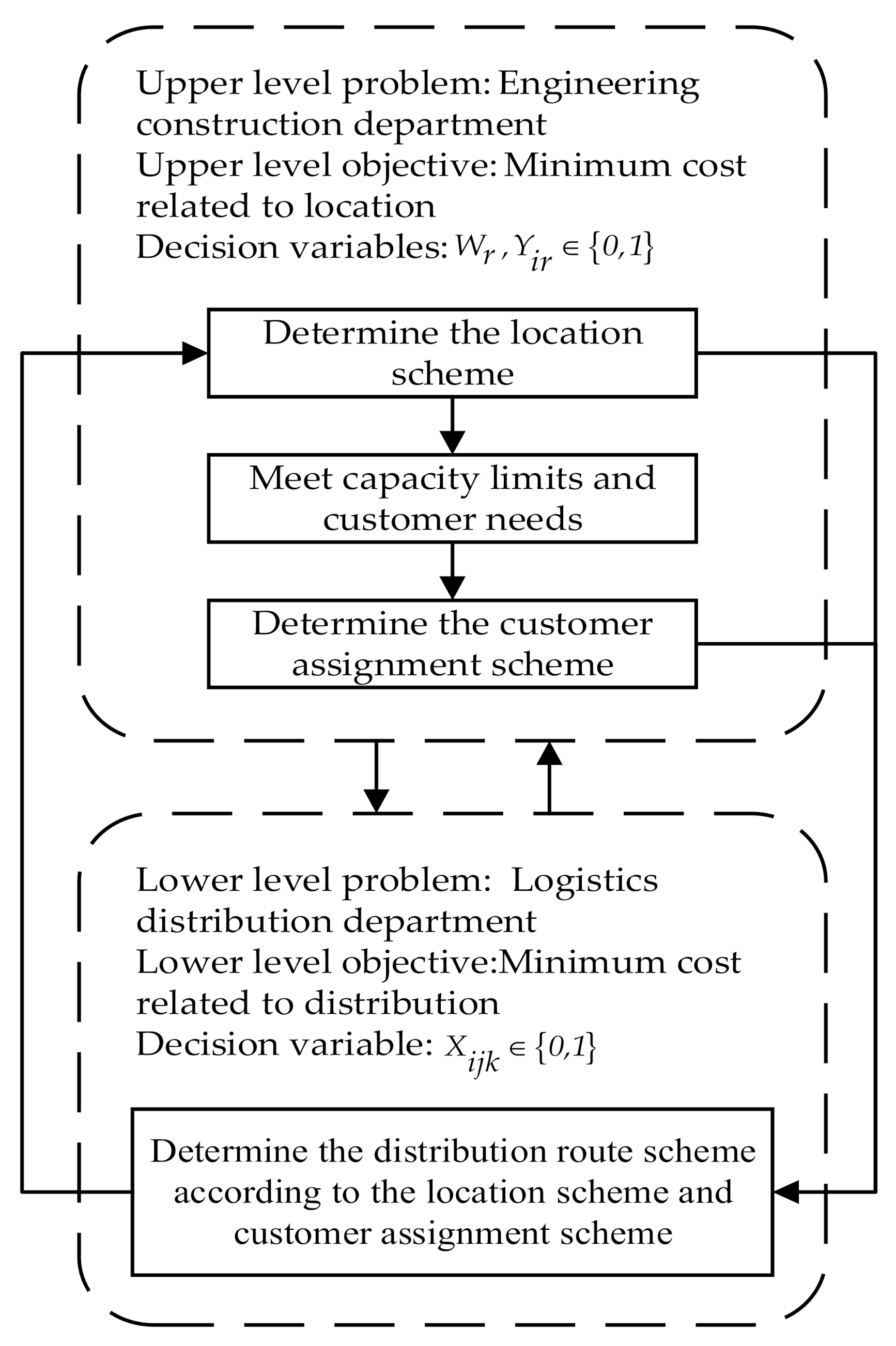
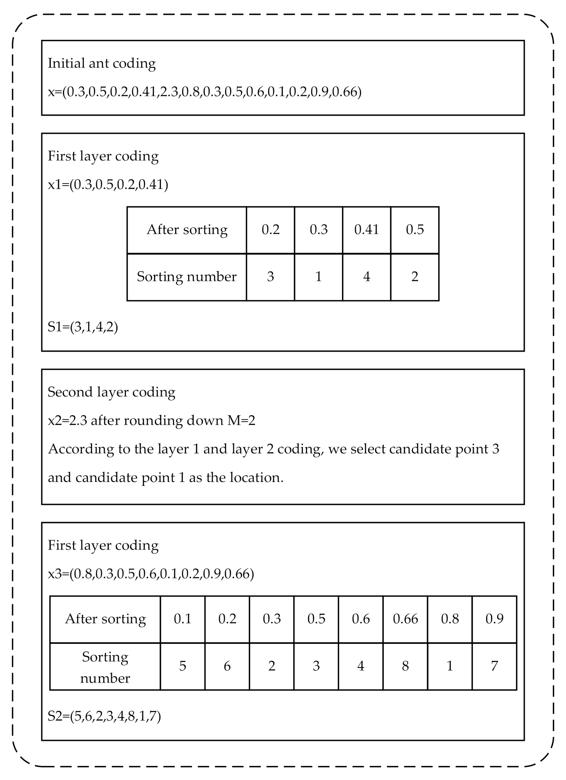
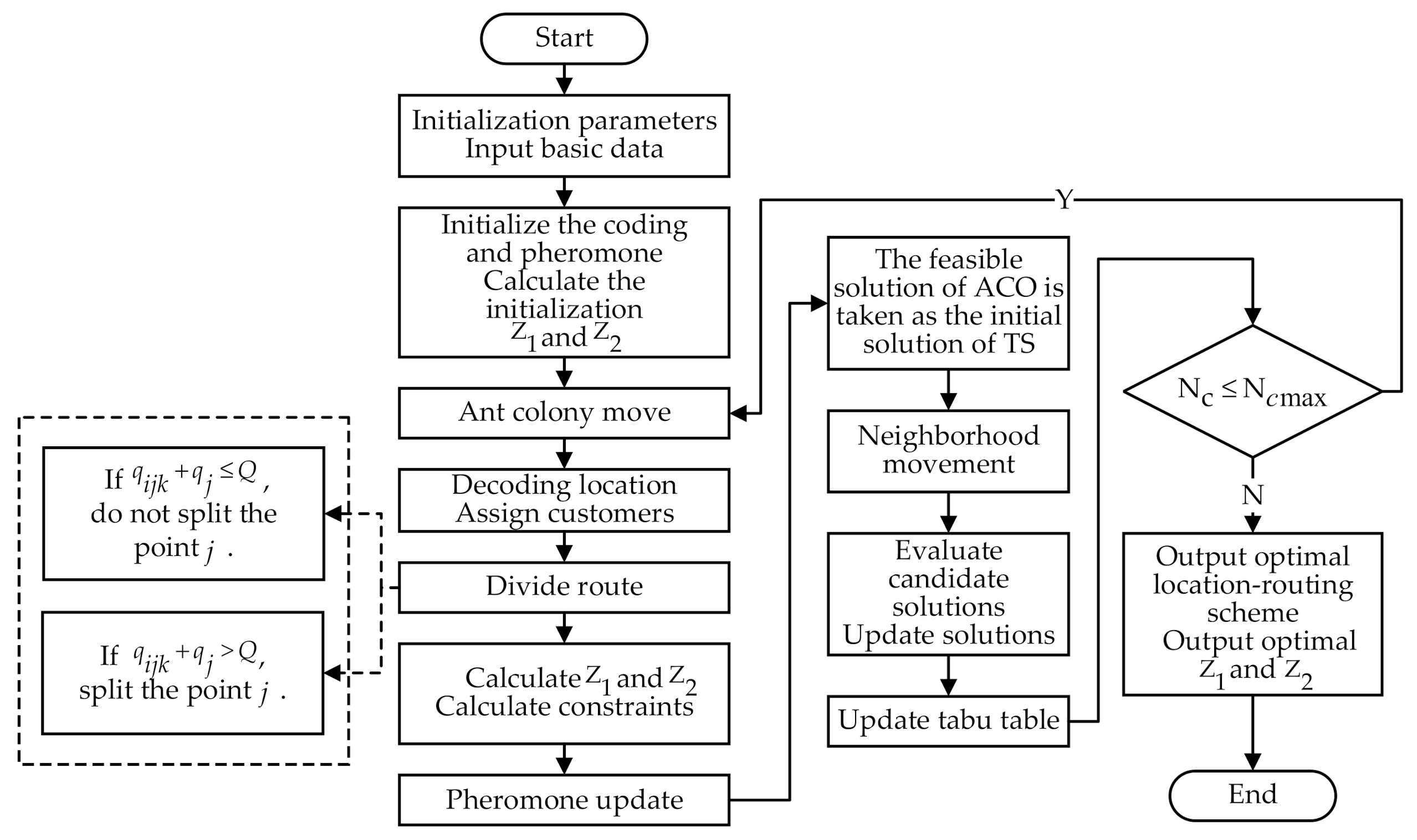
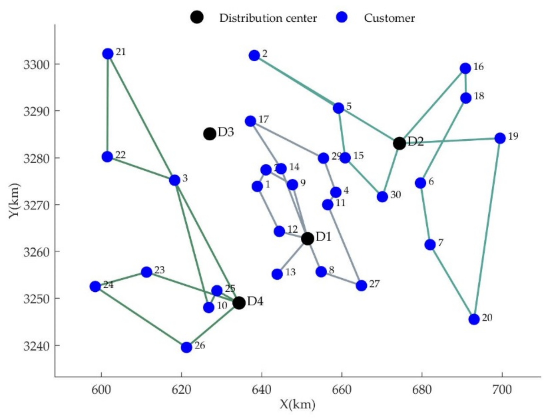
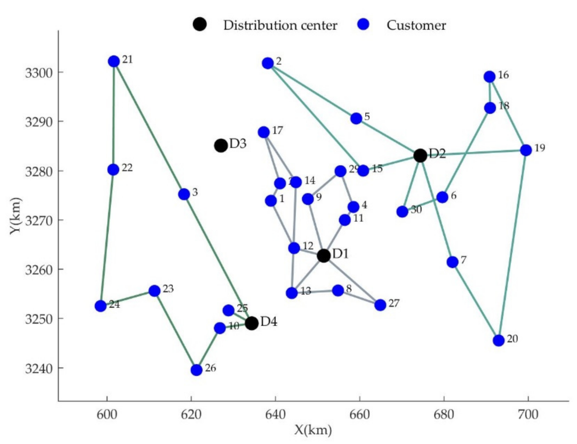
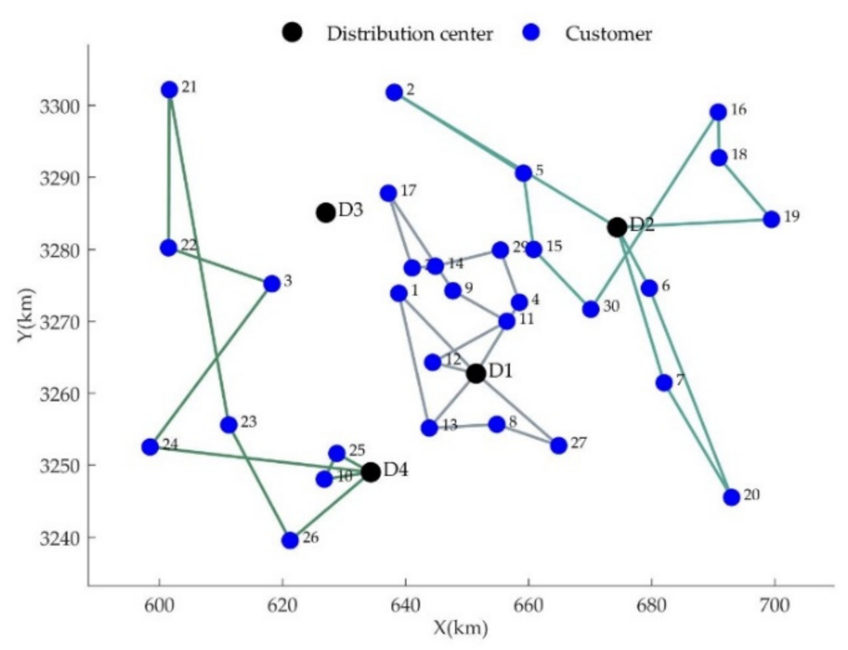
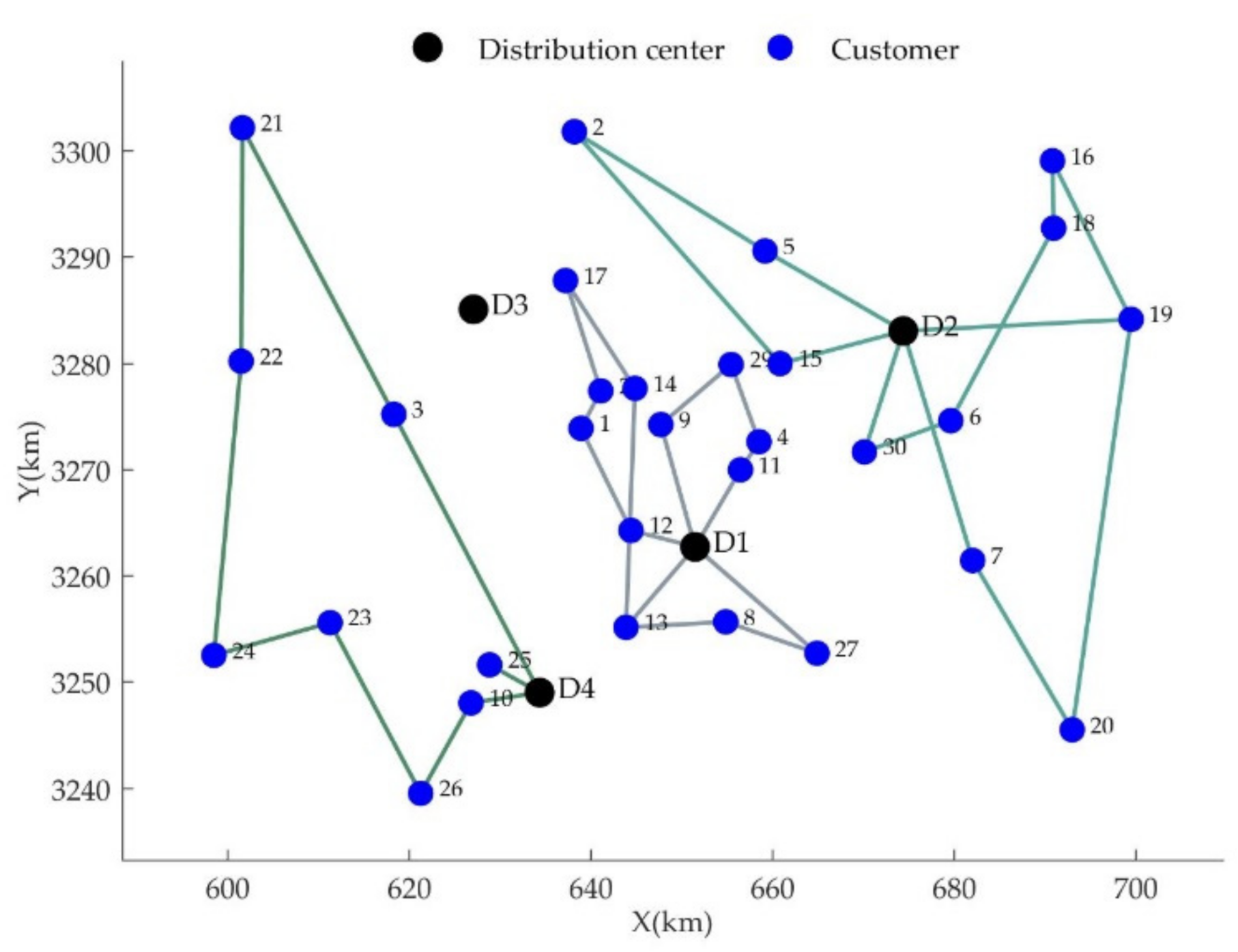
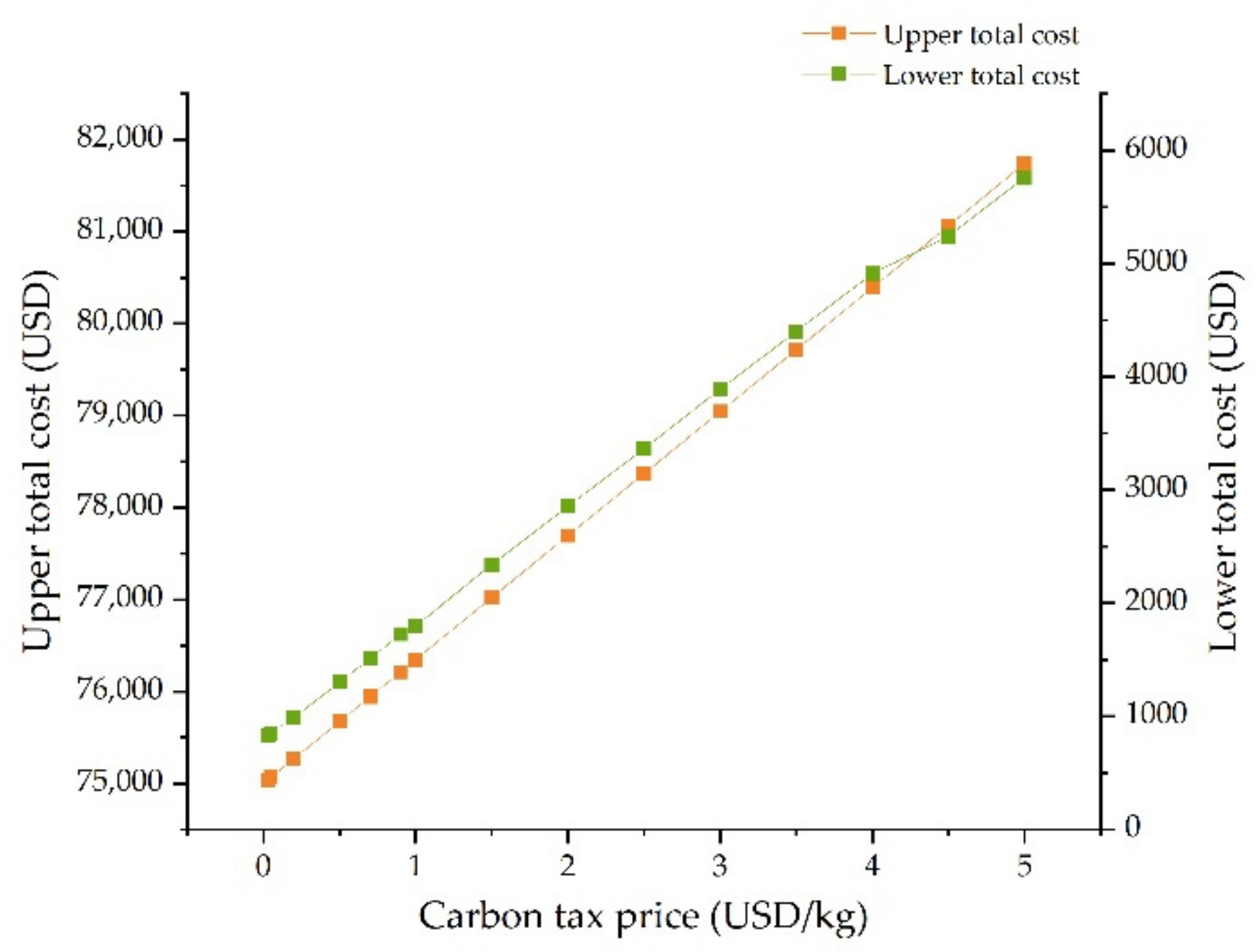
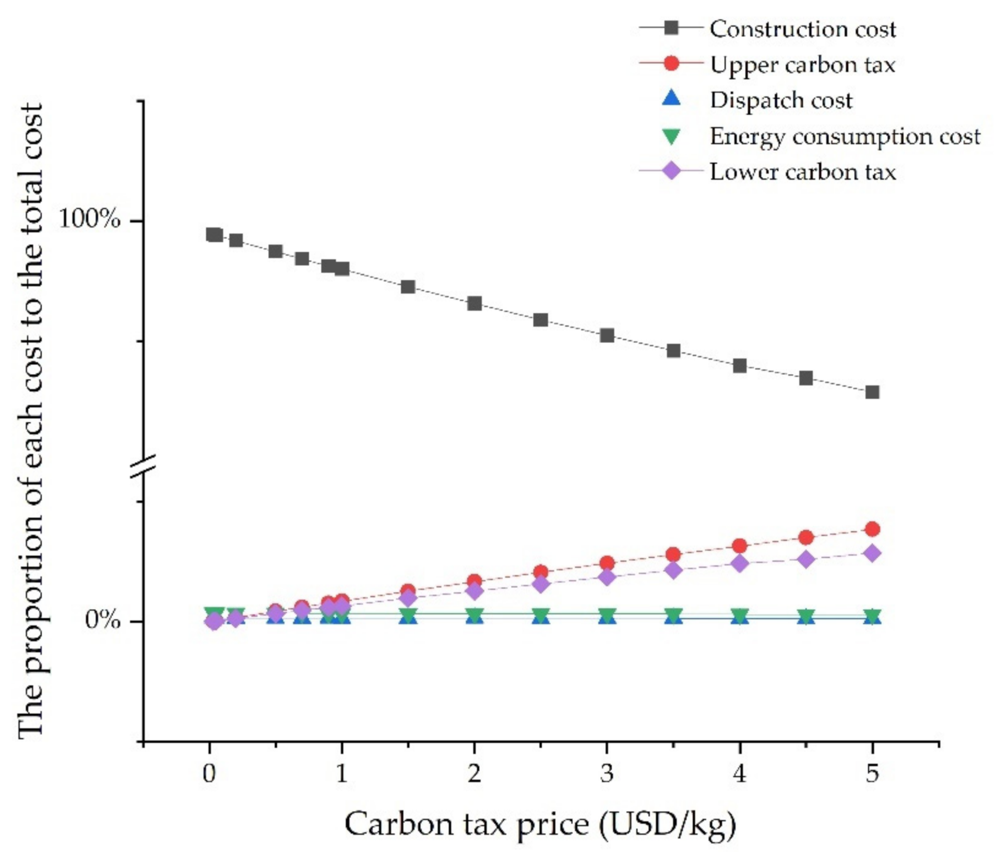
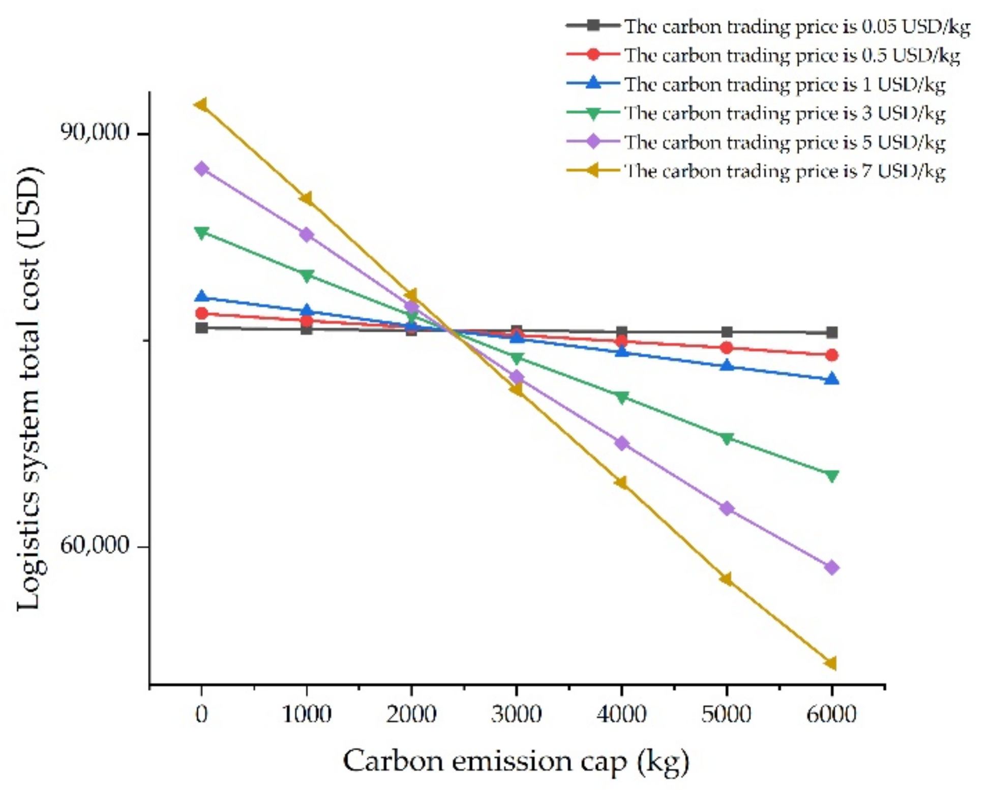
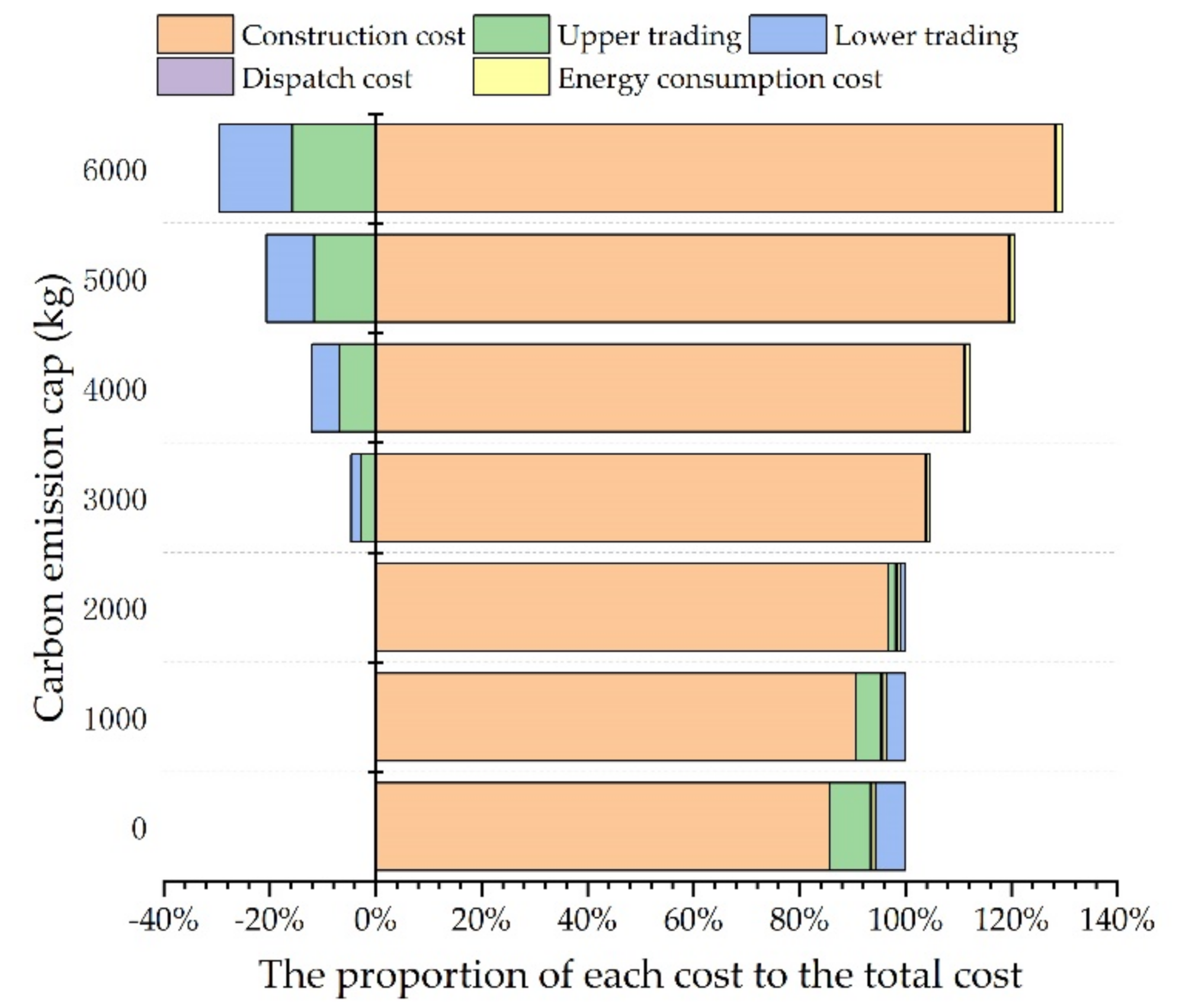
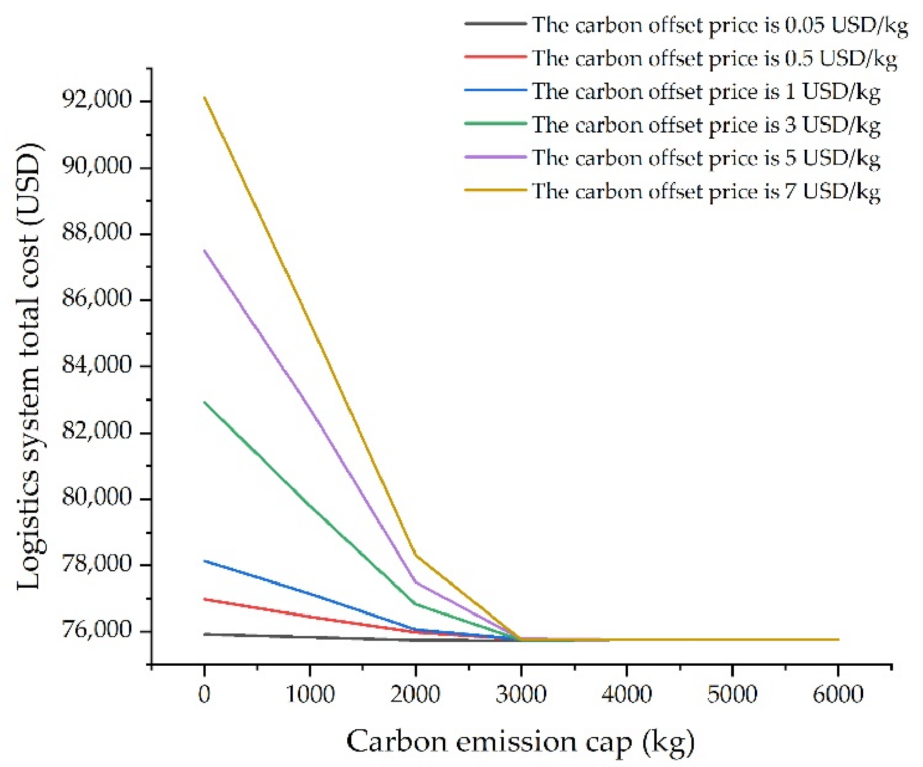
Table 1.
Review of articles on LRP considering carbon emissions.
| Author | Characteristics of the Paper | Algorithm |
|---|---|---|
| Leng et al. [27] | Selection strategy and adaptive acceptance criterion based on sharing mechanism | Hyper-heuristic algorithm |
| Zhang et al. [28] | Uncertain information/carbon emissions | Hybrid intelligent algorithm |
| Chen et al. [29] | Full load problem in regional many-to-many raw material supply network | NSGA-II-TS |
| Koc [30] | Time window/carbon emissions | Adaptive large neighborhood search meta-heuristic algorithm |
| Shen et al. [31] | Demand uncertainty/open location-routing problem | Tabu Search algorithm particle swarm optimization |
| Leng et al. [32] | simultaneous delivery and pick up/time window | Hyper-heuristic method |
| Leng et al. [33] | Multi-objective regional low-carbon LRP | Multi-objective hyper-heuristic method |
| Leng et al. [34] | Cold chain logistics network/customer satisfaction | Multi-objective evolutionary algorithm |
| Araghi et al. [35] | Robust optimization/algorithm application innovation | Hybrid meta-heuristic algorithm |
| Tavana et al. [36] | Location priority/demand uncertainty | Intelligent simulation algorithm |
| Koç et al. [37] | Time window/carbon emission cost | Adaptive large neighborhood search meta-heuristic algorithm |
Table 2.
Abbreviations, sets, parameters, and decision variables.
| Type | Notation | Definitions |
|---|---|---|
| Abbreviations | LRP | The location-routing problem |
| LRPCS | The location-routing problem with cargo splitting | |
| SDVRP | The split delivery vehicle routing problem | |
| ACO | The Ant Colony Optimization | |
| TS | The Tabu Search | |
| ACO-TS | The hybrid algorithm of Ant Colony Optimization and Tabu Search | |
| LP | The location problem | |
| VRP | The vehicle routing problem | |
| EC | The bi-level programming model of the location-routing problem with cargo splitting under the emission cap policy | |
| CS | The bi-level programming model of the location-routing problem with cargo splitting under the carbon tax policy | |
| CT | The bi-level programming model of the location-routing problem with cargo splitting under the carbon trading policy | |
| CO | The bi-level programming model of the location-routing problem with cargo splitting under the carbon offset policy | |
| LC | The bi-level programming model of the location-routing problem with cargo splitting under the low-carbon policy | |
| Sets | The set of all candidate distribution centers, | |
| The set of all distribution vehicles, | ||
| The set of all customers, | ||
| Parameters | The construction and operation cost of distribution center (USD) | |
| The distribution center’s construction and operation costs | ||
| The capacity of distribution center (ton) | ||
| The carbon emission coefficient per unit capacity of distribution center (kg/L) | ||
| The vehicle capacity (ton) | ||
| The road condition coefficient | ||
| The vehicle type correlation coefficient | ||
| The greenhouse gas emission coefficient (kg/L) | ||
| The vehicle net weight (ton) | ||
| The customer demand of (ton) | ||
| The loading capacity of vehicle from to (ton) | ||
| The distance from to (km) | ||
| The speed of vehicle from to (km/h) | ||
| The oil consumption of vehicle from to (L) | ||
| The fuel price (USD/L) | ||
| The demand of customer loaded by vehicle (ton) | ||
| The energy consumption costs of vehicle from to (USD) | ||
| The dispatch costs of vehicle from to (USD) | ||
| The dispatch cost per unit time of vehicle (USD) | ||
| The carbon emission quota under emission cap policy (kg) | ||
| The total carbon emissions generated in distribution process (kg) | ||
| The total carbon emissions from distribution centers (kg) | ||
| The carbon tax (USD/kg) | ||
| The carbon trading price (USD/kg) | ||
| The carbon emission quota under carbon trading policy (kg) | ||
| The carbon emission quota purchased under the carbon trading policy (kg) | ||
| The carbon offset price (USD/kg) | ||
| The carbon emission cap under the carbon offset policy (kg) | ||
| The amount of carbon emission offset under the carbon offset policy (kg) | ||
| The parameter that measures whether traffic is congested or not | ||
| Decision variables | If location is selected to build a distribution center, this variable takes the value 1, and otherwise it takes the value 0 | |
| If the customer is served by distribution center , this variable takes the value 1, and otherwise it takes the value 0 | ||
| If the vehicle travels from node to node , this variable takes the value 1, and otherwise it takes the value 0 |
Table 3.
Candidate distribution center data.
| Distribution Center | X (km) | Y (km) | Construction and Operation Cost (USD) | Capacity (ton) |
|---|---|---|---|---|
| 1 | 651.49 | 3262.69 | 30,000 | 16 |
| 2 | 674.4 | 3283.02 | 27,000 | 18 |
| 3 | 627.1 | 3285.06 | 27,000 | 15 |
| 4 | 634.39 | 3248.97 | 18,000 | 12 |
Table 4.
The customer data.
| Customer | X (km) | Y (km) | Demand (ton) |
|---|---|---|---|
| 1 | 638.94 | 3273.85 | 0.45 |
| 2 | 638.2 | 3301.79 | 0.5 |
| 3 | 618.34 | 3275.17 | 0.4 |
| 4 | 658.53 | 3272.59 | 0.25 |
| 5 | 659.19 | 3290.56 | 1.2 |
| 6 | 679.63 | 3274.57 | 0.6 |
| 7 | 682.03 | 3261.41 | 0.9 |
| 8 | 654.87 | 3255.63 | 0.75 |
| 9 | 647.72 | 3274.21 | 0.8 |
| 10 | 626.83 | 3248 | 0.55 |
| 11 | 656.49 | 3269.95 | 0.4 |
| 12 | 644.44 | 3264.24 | 1.35 |
| 13 | 643.89 | 3255.11 | 5.5 |
| 14 | 644.88 | 3277.62 | 0.15 |
| 15 | 660.84 | 3279.95 | 0.7 |
| 16 | 690.82 | 3299.04 | 0.45 |
| 17 | 637.24 | 3287.77 | 0.8 |
| 18 | 690.95 | 3292.71 | 0.25 |
| 19 | 699.47 | 3284.12 | 5.6 |
| 20 | 692.99 | 3245.47 | 0.55 |
| 21 | 601.68 | 3302.16 | 0.4 |
| 22 | 601.54 | 3280.18 | 1.2 |
| 23 | 611.33 | 3255.55 | 0.5 |
| 24 | 598.54 | 3252.48 | 0.9 |
| 25 | 628.88 | 3251.58 | 6 |
| 26 | 621.29 | 3239.48 | 0.8 |
| 27 | 664.91 | 3252.67 | 0.6 |
| 28 | 641.11 | 3277.38 | 0.3 |
| 29 | 655.45 | 3279.86 | 0.8 |
| 30 | 670.12 | 3271.63 | 0.7 |
Table 5.
The example parameters.
| Parameter | Symbol | Numerical Value |
|---|---|---|
| Carbon emission coefficient per unit capacity of distribution center | 29.3 kg/L | |
| Vehicle capacity | 5 ton | |
| Vehicle net weight | 2 ton | |
| Fuel price | 1.2 USD/L | |
| Vehicle dispatch fee per unit time | 16 USD/h |
Table 6.
Algorithm parameters.
| Parameter | Numerical Value |
|---|---|
| Maximum number of iterations | 250 |
| Ant population | 150 |
| Pheromone volatilization coefficient | 0.1 |
| Pheromone enhancement factor | 1 |
| Ant crawling speed | 0.05 |
| Tabu table length | 40 |
Table 7.
The result of location-routing scheme with and without cargo splitting.
| Scenario | Construction Cost (USD) | DC Carbon Emission (kg) | Dispatch Cost (USD) | Energy Consumption Cost (USD) | Distribution Carbon Emissions (kg) | Location Decision | DC Handling Capacity (ton) |
|---|---|---|---|---|---|---|---|
| Cargo without splitting | 75,000 | 1347.8 | 255.98 | 534.26 | 1032.91 | 1/2/4 | 12.15/11.45/10.75 |
| Cargo with splitting | 75,000 | 1347.8 | 228.32 | 523.44 | 1011.99 | 1/2/4 | 12.15/11.45/10.75 |
| Saving rate | 0.00% | 0.00% | 10.81% | 2.03% | 2.03% | / | / |
Table 8.
Comparison of carbon emissions considering traffic congestion or not in the case of cargo splitting.
Table 8.
Comparison of carbon emissions considering traffic congestion or not in the case of cargo splitting.
| Scenario | Construction Cost (USD) | DC Carbon Emission (kg) | Dispatch Cost (USD) | Energy Consumption Cost (USD) | Distribution Carbon Emissions (kg) |
|---|---|---|---|---|---|
| Yes | 75,000 | 1347.8 | 257.43 | 550.29 | 1063.90 |
| No | 75,000 | 1347.8 | 228.32 | 523.44 | 1011.99 |
Table 9.
Comparison of carbon emissions with and without cargo splitting considering traffic congestion.
Table 9.
Comparison of carbon emissions with and without cargo splitting considering traffic congestion.
| Scenario | Construction Cost (USD) | DC Carbon Emission (kg) | Dispatch Cost (USD) | Energy Consumption Cost (USD) | Distribution Carbon Emissions (kg) |
|---|---|---|---|---|---|
| Yes | 75,000 | 1347.8 | 257.43 | 550.29 | 1063.90 |
| No | 75,000 | 1347.8 | 232.25 | 532.94 | 1030.36 |
Table 10.
Comparison of solution efficiency between ACO-TS and ACO.
| Algorithm | Construction Cost (USD) | DC Carbon Emission (kg) | Dispatch Cost (USD) | Energy Consumption Cost (USD) | Distribution Carbon Emissions (kg) |
|---|---|---|---|---|---|
| ACO | 75,000 | 1347.8 | 252.81 | 583.53 | 1128.15 |
| ACO-TS | 75,000 | 1347.8 | 228.32 | 523.44 | 1011.99 |
| Saving rate | 0 | 0 | 9.69% | 10.3% | 10.3% |
Table 11.
Location-routing results under different carbon emissions caps.
| Cap (kg) | Upper Total Cost (USD) | Lower Total Cost (USD) | Construction Cost (USD) | DC Carbon Emission (kg) | Dispatch Cost (USD) | Energy Consumption Cost (USD) | Distribution Carbon Emissions (kg) |
|---|---|---|---|---|---|---|---|
| 0–2372.85 | / | / | / | / | / | / | / |
| 2372.86–6000 | 75,000 | 758.17 | 75,000 | 1347.8 | 227.99 | 530.2 | 1025.05 |
Table 12.
The relationship between total cost and total carbon emission and carbon trading.
| Carbon Trading Price (USD/kg) | Cap (kg) | Total Carbon Emission (kg) | Total Cost (USD) |
|---|---|---|---|
| 0.05 | 0 | 2416.39 | 75,918.92 |
| 1000 | 2356.50 | 75,824.46 | |
| 2000 | 2326.02 | 75,740.59 | |
| 3000 | 2360.53 | 75,733.60 | |
| 4000 | 2334.36 | 75,665.24 | |
| 5000 | 2369.62 | 75,634.13 | |
| 6000 | 2361.82 | 75,589.02 | |
| 0.5 | 0 | 2396.07 | 76,974.76 |
| 1000 | 2370.39 | 76,452.01 | |
| 2000 | 2401.51 | 75,983.69 | |
| 3000 | 2341.69 | 75,421.51 | |
| 4000 | 2363.90 | 74,944.65 | |
| 5000 | 2402.83 | 74,492.75 | |
| 6000 | 2377.38 | 73,945.56 | |
| 1 | 0 | 2380.48 | 78,142.28 |
| 1000 | 2376.29 | 77,143.81 | |
| 2000 | 2332.61 | 76,059.78 | |
| 3000 | 2364.10 | 75,135.99 | |
| 4000 | 2367.24 | 74,136.76 | |
| 5000 | 2368.16 | 73,126.85 | |
| 6000 | 2405.62 | 72,182.64 | |
| 3 | 0 | 2384.26 | 82,929.94 |
| 1000 | 2343.59 | 79,787.37 | |
| 2000 | 2354.24 | 76,828.14 | |
| 3000 | 2350.49 | 73,811.49 | |
| 4000 | 2387.215469 | 70,949.81 | |
| 5000 | 2398.645212 | 67,970.69 | |
| 6000 | 2471.73856 | 65,267.66 | |
| 5 | 0 | 2348.56 | 87,497.40 |
| 1000 | 2389.33 | 82,723.63 | |
| 2000 | 2347.29 | 77,492.14 | |
| 3000 | 2326.02 | 72,354.39 | |
| 4000 | 2365.14 | 67,583.22 | |
| 5000 | 2402.31 | 62,800.40 | |
| 6000 | 2534.36 | 58,535.47 | |
| 7 | 0 | 2342.258 | 92,136.35 |
| 1000 | 2366.42 | 85,321.37 | |
| 2000 | 2361.84 | 78,300.65 | |
| 3000 | 2382.26 | 71,455.37 | |
| 4000 | 2414.14 | 64,686.35 | |
| 5000 | 2412.14 | 57,672.84 | |
| 6000 | 2528.50 | 51,567.05 |
Publisher’s Note: MDPI stays neutral with regard to jurisdictional claims in published maps and institutional affiliations. |
© 2021 by the authors. Licensee MDPI, Basel, Switzerland. This article is an open access article distributed under the terms and conditions of the Creative Commons Attribution (CC BY) license (https://creativecommons.org/licenses/by/4.0/).
Share and Cite
MDPI and ACS Style
Wang, C.; Peng, Z.; Xu, X. A Bi-Level Programming Approach to the Location-Routing Problem with Cargo Splitting under Low-Carbon Policies. Mathematics 2021, 9, 2325. https://0-doi-org.brum.beds.ac.uk/10.3390/math9182325
AMA Style
Wang C, Peng Z, Xu X. A Bi-Level Programming Approach to the Location-Routing Problem with Cargo Splitting under Low-Carbon Policies. Mathematics. 2021; 9(18):2325. https://0-doi-org.brum.beds.ac.uk/10.3390/math9182325
Chicago/Turabian StyleWang, Cong, Zhongxiu Peng, and Xijun Xu. 2021. "A Bi-Level Programming Approach to the Location-Routing Problem with Cargo Splitting under Low-Carbon Policies" Mathematics 9, no. 18: 2325. https://0-doi-org.brum.beds.ac.uk/10.3390/math9182325
Note that from the first issue of 2016, this journal uses article numbers instead of page numbers. See further details here.