An Integrated Mathematical Attitude Utilizing Fully Fuzzy BWM and Fuzzy WASPAS for Risk Evaluation in a SOFC

Abstract

Nowadays, because of the energy crisis, combined heat and power systems have notable benefits. One of the best devices is SOFC (Solid Oxide Fuel Cell) which joins heat and power frameworks. Some considerable failure modes arise that can affect these devices’ productivity. Generally, failure modes evaluations need an experts team to achieve uncertainties belongs to the risk assessment procedure. To improve the efficiency of the routine FMEA methodology and to represent a suitable hybrid fuzzy MCDM approach for FMEA, in this work, fully fuzzy best-worst method (FF-BWM) is employed to achieve the risk factors weights then fuzzy weighted aggregated sum product assessment (F-WASPAS) approach to detect the failure modes priorities is utilized. Ultimately, the sensitivity analyses demonstrate that the offered framework is verified and can make applicable data in risk management decision-making evaluation.

1. Introduction

The consistent improvement in industries causes a huge expansion in energy interest. In this way, expanding nature-accommodating devices with high proficiency is imperative to limit the adverse consequences of non-renewable energy sources [1]. The synthetic energy of vaporous or liquid reactants can be transformed into electricity employing sorts of devices called fuel cells [2]. Each fuel cell includes a special electrolyte layer segregating reactants from chemically reacting. This layer is regarding porous cathode and anode parts [3]. Fuel cells have various categories that the Solid Oxide Fuel Cells (SOFCs) have drawn into incredible consideration in recent years [4]. Guk et al. [5] expressed that for acquiring better knowledge into the SOFC efficiency, the most significant factor to consider is the electrode temperature dispensation. In this way, to gauge the cathode and anode temperature dispensation from a functioning SOFC, they introduced a new cell-incorporated multi-intersection thermocouple cluster. Gallo et al. [6] proposed a new strategy to prognosticate the SOFC staying valuable life. Kong et al. [7] investigated numerically a two dimensional configuration of a SOFC. They utilized a heat bar in their model and compared it to a model without that heat bar and analyzed the impact of heat bar on the cell proficiency. Xu et al. [8] simulated an SOFC with methanol as fuel. Their modeling was a 2D simulation and they represented the effect of some important factors on the cell efficiency. Wang et al. [9] could increase outcome hydrogen to 80% which was 14% higher than the yield of conventional SOFC. They also could decrease the operation cost. Zaghloul et al. [10] described a novel strategy to measure cell temperature. Thus, they could record a suitable temperature change on the electrodes.

An MCDM approach is made of several alternatives and objectives. These methodologies can incorporate penalty function, weighted-aggregate, objective programming, and fuzzy methods [11]. This issue has attracted lots of investigators. In the last years, several MCDM methods introduced to evaluate the criteria weight or alternative ranking. The weighting methods include analytic hierarchy process (AHP) [12], which contains three parts: the ultimate goal or problem it is supposed to be solved, all of the possible solutions, called alternatives, and the criteria one will judge the alternatives on, analytic network process (ANP) [13], which is an attempt to improve AHP based on the analysis conducted by the human brain for complicated issues with non-hierarchical structures, step-wise weight assessment ratio analysis (SWARA) [14], in which the relative importance and the initial prioritization of alternatives for each attribute are determined by the opinion of the decision maker, and finally, the relative weight of each attribute is determined, best-worst method (BWM) [15], which is a pairwise comparison-based method that offers a structured way to make the comparisons, full consistency method (fucom) [16] which is a semi-objective/objective evaluation method, which reduces the comparison of criteria within each other and optimizes the criteria weights with the optimization algorithm with few comparisons, and base-criterion method (BCM) [17] in which one of the criteria is chosen by the decision-maker as a base-criterion and then pairwise comparisons between base-criterion and other criteria are obtained. Then, a max-min problem is formulated and solved to determine the weight of the criteria.

Also, MCDM methods for alternatives ranking include techniques for order of preference by similarity to ideal solution (TOPSIS) [18], which is based on the idea that the best alternatives should have the farthest distance from the negative ideal solution and the shortest distance from the positive ideal solutions, vlseKriterijumska optimizacija i kompromisno resenje (VIKOR) [19], which determines the compromise ranking list and the compromise solution obtained with the initial weights focusing on ranking and selecting from a set of alternatives in the presence of conflicting criteria, multi-objective optimization method by ratio analysis (MOORA) [20], which is considered as an objective (non-subjective) method. Moreover, desirable and undesirable criteria are used simultaneously for ranking to select a superior or higher alternative among different alternatives, complex proportional assessment (COPRAS) [21], which is utilized to assess the maximizing and minimizing index values, and the effect of maximizing and minimizing indexes of attributes on the results assessment is considered separately, weighted aggregated sum product assessment (WASPAS) [22] which is a combination of weighted sum model (WSM) and weighted product model (WPM), a technique through which the relative importance of each attribute is simply determined and the alternatives are evaluated and prioritized, combined compromise solution (CoCoSo) method [23], which is based on an integrated simple additive weighting and exponentially weighted product model and Grey relational analysis (GRA), originally proposed by [24], which aims to show the degree of similarity or difference of development trends between an alternative and the reference (ideal) alternative [25], and some other methods.

The BWM and WASPAS methods have been used successfully in various scientific fields [26,27,28,29,30]. Zavadskas et al. [22] introduced the WASPAS method to improve the accuracy of alternatives ranking. This method is a combination of the weighted sum model (WSM) and weighted product model (WPM). Also, Ref. [31] extended the WASPAS with interval-valued intuitionistic fuzzy numbers. Turskis et al. [26] proposed a fuzzy WASPAS to select the best shopping center. Gundogdu and Kahraman [32] extended WASPAS in a spherical fuzzy environment. Rudnik et al. [33] proposed another extension of the WASPAS using the Ordered Fuzzy Numbers.

Rezaei [15] introduced the BWM as a powerful MCDM method to obtain the criteria weight. The BWM is vector-based and used pairwise comparisons to evaluate the opinions of decision-makers [34]. The BWM compared to other similar methods requires fewer pairwise comparisons [35]. In recent years, the BWM has been developed by researchers the various fields, such as intuitionistic fuzzy multiplicative BWM [36], fuzzy BWM [37], interval-valued fuzzy-rough BWM [16], Z-BWM [38], piecewise linear fuzzy BWM [39], Interval-valued pythagorean hesitant fuzzy BWM [40], FMEA-BWM [39,41], Bayesian BWM [42], rough-fuzzy BWM [43], trapezoidal fuzzy BWM [44], BWM with D-number [45], modified fuzzy BWM [46], group BWM [47] and fully fuzzy BWM [48].

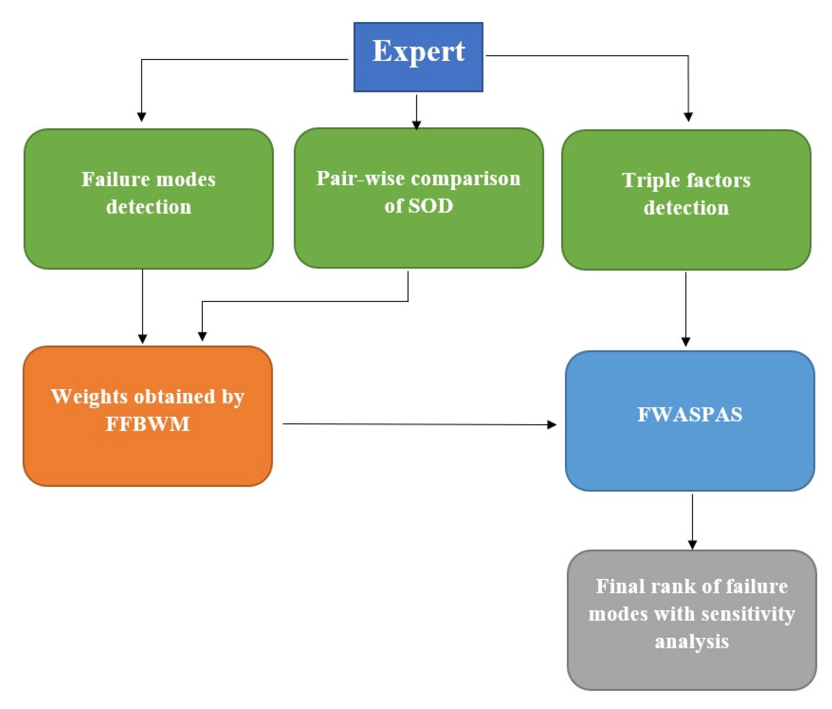
In the fully fuzzy methodology, all feasible pairwise comparisons were not required. The ff- BWM has provided high reliability to the results. This method is independent with its high capability to hybrid other MCDM methods. Therefore, the present work is an extended investigation of precise and hybrid fuzzy MCDM methods for risk evaluation by utilizing fully fuzzy BWM and fuzzy WASPAS to extract an appropriate risk ranking. The key contributions of this work are to deduce the risk factors’ weight, fully fuzzy BWM as a linear mathematical model is used. The next novelty is that to achieve the risk scores of potential failure modes, fuzzy WASPAS technique is utilized to clarify the failure modes ranking. Finally, the suggested approach is employed to evaluate a ceramic anode solid oxide fuel cell and a sensitivity evaluation is derived.

Considering all mentioned points, this paper consists of several sections as follows: Section 2 is about methodology including FF-BWM and F-WASPAS. Section 3 and Section 4 represent the suggested approach and introduced the main case study, respectively. Ultimately, Section 5 concluded the results.

2. Methodology

In this part of the research, the principles of fuzzy logic, FF-BWM, and F-WASPAS are reviewed.

2.1. Fuzzy Logic

2.1.1. Triangular Fuzzy Numbers (TFNs)

Ref. [49], the first investigator, described the fuzzy set hypothesis. At that point, this concept was spread in various fields of study by numerous researchers. The membership function ${\mu }_{\tilde{A}}:Y\to [0,1]$ is characterized for the TFNs $\tilde{A}=(a^1,a^2,a^3)$ and is achieved as follows [50]:

$${\mu }_{\tilde{A}}\left(y\right)=\left\{\begin{array}{cc}\frac{y-a^1}{a^2-a^1}\hfill & a^1\le y\le a^2\hfill \\ \frac{a^3-y}{a^3-a^2}\hfill & a^2\le y\le a^1\hfill \\ 0\hfill & \mathrm{otherwise}.\hfill \end{array}\right.$$

(1)

Main components of the TFNs $\tilde{A}=(a^1,a^2,a^3)$ are the left bound $\left(a^1\right)$, the center $\left(a^2\right)$, and the right bound $\left(a^3\right)$, individually. Some mathematical principles for two TFNs $(a_1^1,a_1^2,a_1^3)$ and $(a_2^1,a_2^2,a_2^3)$ are also introduced as follows [51]:

$$\begin{array}{c}\hfill \begin{array}{cc}\hfill \left(\mathrm{i}\right)\mathrm{Addition}:& (a_1^1,a_1^2,a_1^3)\oplus (a_2^1,a_2^2,a_2^3)=(a_1^1+a_2^1,a_1^2+a_2^2,a_1^3+a_2^3)\hfill \end{array}\end{array}$$

(2)

$$\begin{array}{c}\hfill \begin{array}{cc}\hfill \left(\mathrm{ii}\right)\mathrm{Subtraction}:& (a_1^1,a_1^2,a_1^3)\exists (a_2^1,a_2^2,a_2^3)=(a_1^1-a_2^3,a_1^2-a_2^2,a_1^3-a_2^1)\hfill \end{array}\end{array}$$

(3)

$$\begin{array}{cc}\hfill \left(\mathrm{iii}\right)\mathrm{Multiplication}:& (a_1^1,a_1^2,a_1^3)\otimes (a_2^1,a_2^2,a_2^3)=(a_1^1{a}_2^1,a_1^2{a}_2^2,a_1^3{a}_2^3)\hfill \end{array}$$

(4)

$$\begin{array}{cc}\hfill \left(\mathrm{iv}\right)\mathrm{Divition}:& (a_1^1,a_1^2,a_1^3)\%(a_2^1,a_2^2,a_2^3)=\left(\frac{a_1^1}{a_2^3},\frac{a_1^2}{a_2^2},\frac{a_1^3}{a_2^1}\right)\hfill \end{array}$$

(5)

$$\begin{array}{cc}\hfill \left(\mathrm{v}\right)\mathrm{Power}:& (a_1^1,a_1^2,a_1^3){⊛}^{(a_2^1,a_2^2,a_2^3)}=(a_1^{1^{a_2^1}},a_1^{2^{a_2^2}},a_1^{3^{a_2^3}})\hfill \end{array}$$

(6)

The mentioned operational principles are fuzzy number addition, subtraction, multiplication, division, and power, separately.

2.1.2. Fully Fuzzy Best Worst Method (FF-BWM)

During this procedure, the BWM is introduced in a fuzzy environment. This process includes four steps: step 1 consists of decision makers’ team selection, step 2 is the best and worst criteria detection by decision makers’ team, step 3 is pairwise comparisons covering the best criterion to other criteria and the other criteria to the worst criterion, and ultimately step 4 is fuzzy optimal weights calculation. It should be noted that after step 4, the mathematical model conversion to linear ranking function is performed. These steps are represented as follows:

Step 1.

Generating a system of decision objectives:

• An alternative according to some criteria must be chosen by the Decision Maker (DM) in an MCDM. Consider the set of n criteria is $\{c_1,c_2,\dots ,c_n\}$.

Step 2.

The best and the worst criterion detection:

• During this stage, the best $c_B$ and the worst $c_W$ criteria should be chosen by DM.

Step 3.

Fuzzy reference comparison:

• This step includes a comparison between the best criterion and other criteria and also, between the worst criterion and others. The results of this process are represented in Equations (7) and (8).

$${\tilde{A}}_B=({\tilde{a}}_{B1},{\tilde{a}}_{B2},\cdots ,{\tilde{a}}_{Bn})$$

(7)

$${\tilde{A}}_W=({\tilde{a}}_{1W},{\tilde{a}}_{2W},\cdots ,{\tilde{a}}_{nW})$$

(8)

Step 4.

Computation of the favorable fuzzy weights:

• The optimal quantity of ${\tilde{w}}_B\%{\tilde{w}}_j$ and ${\tilde{w}}_j\%{\tilde{w}}_W$ give the components of the comparison matrix ${\tilde{w}}_B\%{\tilde{w}}_j={\tilde{a}}_{Bj},{\tilde{w}}_j\%{\tilde{w}}_W={\tilde{a}}_{jW}$. It is vital to minimize the maximum absolute value of $|{\tilde{w}}_B\%{\tilde{w}}_j\exists {\tilde{a}}_{Bj}|$ and $|{\tilde{w}}_j\%{\tilde{w}}_W\exists {\tilde{a}}_{jW}|$ for each j to achieve the optimal weights $({\tilde{w}}_1^{\ast },{\tilde{w}}_2^{\ast },\cdots ,{\tilde{w}}_n^{\ast })$. This procedure is represented as follows:

$$Min\left\{Max\right\{|{\tilde{w}}_B\%{\tilde{w}}_j\exists {\tilde{a}}_{Bj}|,|{\tilde{w}}_j\%{\tilde{w}}_W\exists {\tilde{a}}_{jW}\left|\right\}\}$$

(9)

$$\begin{array}{c}\hfill \begin{array}{cc}\hfill subjectto:& \sum _{j=1}^n{\tilde{w}}_j=\tilde{1}\hfill \end{array}\end{array}$$

(10)

$$\begin{array}{c}\hfill \begin{array}{cc}\hfill & {\tilde{w}}_j\ge \tilde{0}\hfill \end{array}\end{array}$$

(11)

$$\begin{array}{cc}\hfill & j=1,2,\cdots ,n\hfill \end{array}$$

(12)

Equation (9) can be linearized as follows [48]:

$$\begin{array}{c}\hfill \begin{array}{cc}\hfill Min& \tilde{\theta }\hfill \end{array}\end{array}$$

(13)

$$\begin{array}{c}\hfill \begin{array}{cc}\hfill subjectto:& \tilde{\theta }\ge {\tilde{w}}_B\exists {\tilde{w}}_j\otimes {\tilde{a}}_{Bj}\hfill \end{array}\end{array}$$

(14)

$$\begin{array}{c}\hfill \begin{array}{cc}\hfill & \tilde{\theta }\ge {\tilde{w}}_j\otimes {\tilde{a}}_{Bj}\exists {\tilde{w}}_B\hfill \end{array}\end{array}$$

(15)

$$\begin{array}{c}\hfill \begin{array}{cc}\hfill & \tilde{\theta }\ge {\tilde{w}}_j\exists {\tilde{w}}_W\otimes {\tilde{a}}_{jW}\hfill \end{array}\end{array}$$

(16)

$$\begin{array}{c}\hfill \begin{array}{cc}\hfill & \tilde{\theta }\ge {\tilde{w}}_W\otimes {\tilde{a}}_{jW}\exists {\tilde{w}}_j\hfill \end{array}\end{array}$$

(17)

$$\begin{array}{cc}\hfill & \tilde{\theta }\ge \tilde{0},j=1,2,\cdots ,n\hfill \end{array}$$

(18)

where${\tilde{w}}_j=(w_j^1,w_j^2,w_j^3),{\tilde{w}}_B=(w_B^1,w_B^2,w_B^3),{\tilde{w}}_W=(w_W^1,w_W^2,w_W^3),{\tilde{a}}_{Bj}=(a_{Bj}^1,a_{Bj}^2,a_{Bj}^3),$${\tilde{a}}_{jW}=(a_{jW}^1,a_{jW}^2,a_{jW}^3),\tilde{\theta }=({\theta }^1,{\theta }^2,{\theta }^3)$.

To take care of completely fuzzy linear programming issues, a novel technique with triangular fuzzy numbers was presented by [52]. To change the problem they utilized a linear ranking function. Along these lines, the accompanying condition was utilized to change the problem.

$$\tilde{A}=(a^1-\frac{1}{4}{a}^2+\frac{1}{4}{a}^3,-\frac{1}{4}{a}^1,\frac{1}{4}{a}^1)$$

(19)

Consequently, requirements (13)–(18) are changed into limitations (20)–(40).

$$\begin{array}{cc}\hfill \mathrm{Min}& ({\theta }^1-\frac{1}{4}{\theta }^2+\frac{1}{4}{\theta }^3)\hfill \end{array}$$

(20)

$$\begin{array}{cc}\hfill s.to:& w_B^1-\frac{1}{4}{w}_B^2+\frac{1}{4}{w}_B^3-((a_{Bj}^1+\frac{1}{4}(a_{Bj}^3-a_{Bj}^2))w_j^1-\frac{1}{4}{a}_{Bj}^1{w}_j^1+\frac{1}{4}{a}_{Bj}^1{w}_j^3)\hfill \\ \hfill & \le {\theta }^1-\frac{1}{4}{\theta }^2+\frac{1}{4}{\theta }^3\hfill \end{array}$$

(21)

$$\begin{array}{cc}\hfill & w_B^1-\frac{1}{4}{w}_B^2+\frac{1}{4}{w}_B^3-((a_{Bj}^1+\frac{1}{4}(a_{Bj}^3-a_{Bj}^2))w_j^1-\frac{1}{4}{a}_{Bj}^1{w}_j^1+\frac{1}{4}{a}_{Bj}^1{w}_j^3)\hfill \\ \hfill & \ge -({\theta }^1-\frac{1}{4}{\theta }^2+\frac{1}{4}{\theta }^3)\hfill \end{array}$$

(22)

$$\begin{array}{cc}\hfill & w_j^1-\frac{1}{4}{w}_j^2+\frac{1}{4}{w}_j^3-((a_{jW}^1+\frac{1}{4}(a_{jW}^3-a_{jW}^2))w_W^1-\frac{1}{4}{a}_{jW}^1{w}_W^1+\frac{1}{4}{a}_{jW}^1{w}_W^3)\hfill \\ \hfill & \le {\theta }^1-\frac{1}{4}{\theta }^2+\frac{1}{4}{\theta }^3\hfill \end{array}$$

(23)

$$\begin{array}{cc}\hfill & w_j^1-\frac{1}{4}{w}_j^2+\frac{1}{4}{w}_j^3-((a_{jW}^1+\frac{1}{4}(a_{jW}^3-a_{jW}^2))w_W^1-\frac{1}{4}{a}_{jW}^1{w}_W^1+\frac{1}{4}{a}_{jW}^1{w}_W^3)\hfill \\ \hfill & \ge -({\theta }^1-\frac{1}{4}{\theta }^2+\frac{1}{4}{\theta }^3)\hfill \end{array}$$

(24)

$$\begin{array}{cc}\hfill & \sum _{j=1}^n(w_j^1-\frac{1}{4}{w}_j^2+\frac{1}{4}{w}_j^3)=1\hfill \end{array}$$

(25)

$$\begin{array}{cc}\hfill & w_j^1-\frac{1}{4}{w}_j^2+\frac{1}{4}{w}_j^3\ge 0\hfill \end{array}$$

(26)

$$\begin{array}{cc}\hfill & {\theta }^1-\frac{1}{4}{\theta }^2+\frac{1}{4}{\theta }^3\ge 0\hfill \end{array}$$

(27)

$$\begin{array}{cc}\hfill & w_j^2-w_j^1\ge 0\hfill \end{array}$$

(28)

$$\begin{array}{cc}\hfill & w_j^3-w_j^2\ge 0\hfill \end{array}$$

(29)

$$\begin{array}{cc}\hfill & {\theta }^2-{\theta }^1\ge 0\hfill \end{array}$$

(30)

$$\begin{array}{cc}\hfill & {\theta }^3-{\theta }^2\ge 0\hfill \end{array}$$

(31)

After solving the model addressed in the imperatives (20)–(31), the ideal values of the triangular fuzzy loads are acquired.

2.1.3. Consistency Ratio

An ideal consistency of pairwise collation exists when ${\tilde{a}}_{Bj}\otimes {\tilde{a}}_{jW}={\tilde{a}}_{BW}$. The values of ${\tilde{a}}_{Bj}$ and ${\tilde{a}}_{jW}$ describe the relative fluffy inclination of the better standard over basis and the relative fuzzy inclination of the criterion j over the worst criterion, separately. In addition, the relative fuzzy preference of the best criterion over the worst one is introduced as ${\tilde{a}}_{BW}$. Since there is a feasibility for a criterion j not to be entirely reliable. In this way, it is essential to characterize a consistency proportion to assess the consistency level of pairwise correlation.

In a case that the worth of ${\tilde{a}}_{Bj}\otimes {\tilde{a}}_{jW}$ not equivalent to ${\tilde{a}}_{BW}$, the level of consistency will be decreased. In addition, the greatest irregularity $\tilde{\theta }$ happens when both ${\tilde{a}}_{Bj}$ and ${\tilde{a}}_{jW}$ have acquired their most extreme conceivable worth that is equivalent ${\tilde{a}}_{BW}$. In light of ${\tilde{w}}_B\%{\tilde{w}}_j\otimes {\tilde{w}}_j\%{\tilde{w}}_W={\tilde{w}}_B\%{\tilde{w}}_W$ and the previously mentioned issue, the worth of $\tilde{\theta }$ ought to be added to ${\tilde{a}}_{BW}$ and deducted from ${\tilde{a}}_{Bj}$ and ${\tilde{a}}_{jW}$. This point is shown in Equation (32).

$$({\tilde{a}}_{Bj}\exists \tilde{\theta })\otimes ({\tilde{a}}_{jW}\exists \tilde{\theta })=({\tilde{a}}_{BW}\oplus \tilde{\theta })$$

(32)

It is obvious that the high value of possible inconsistency happens when ${\tilde{a}}_{Bj}={\tilde{a}}_{jW}={\tilde{a}}_{BW}$. Thus, Equation (32) can be rewritten as follows:

$$({\tilde{a}}_{BW}\exists \tilde{\theta })\otimes ({\tilde{a}}_{BW}\exists \tilde{\theta })=({\tilde{a}}_{BW}\oplus \tilde{\theta })$$

(33)

The extended form of Equation (33) is described as Equation (34).

$${\tilde{\theta }}^2\exists (1+2{\tilde{a}}_{BW})\tilde{\theta }\oplus ({\tilde{a}}_{BW}^2\exists {\tilde{a}}_{BW})=\tilde{0}$$

(34)

Equation (34) ought to be solved for various upsides of ${\tilde{a}}_{ij}\in \{1,2,\cdots ,9\}$ to track down the greatest conceivable worth of $\tilde{\theta }$. Therefore, it is introduced as the consistency index (CI) and consistency ratio (CR) can be achieved by ${\theta }^{\ast }$, CI, and the Equation (35).

$$\mathrm{CR}=\frac{{\theta }^{\ast }}{\mathrm{CI}}$$

(35)

It is important to be noted that the fuzzy number ${\theta }^{\ast }$ is changed into a number by taking the average of its components. Thereafter, the acquired number will be utilized in Equation (35).

2.2. Fuzzy WASPAS

Since by utilizing a fuzzy methodology, it is possible to allocate the relative significance of qualities using fuzzy numbers instead of exact numbers, this part stretches out WASPAS to the fuzzy environment. MADM technique, specifically WASPAS, was presented in 2012 [22]. Afterward, alteration of the strategy WASPAS-IFIV was presented [31]. The WASPAS method includes two major steps:

• The Weighted Summation Model (WSM);
• The Weighted Production Model (WPM).

The WSM addresses the general score of an option as a weighted amount of the property estimations. The WPM is created to stay away from the alternatives with poor property estimations. It decides the score of every option as a product of the scale rating of each attribute to power equivalent to the significant weight of the characteristic [53]. Given the momentarily summed up fuzzy hypothesis above, WASPAS-F steps can be illustrated as follows:

Step 1. Fuzzy Decision-Making Matrix (FDMM) generation:

A DMM consists of the performance values ${\tilde{m}}_{ij}$ and the attribute loads ${\tilde{w}}_j$. An expert as DM decides the attributes and initial weights of them. The discrete enhancement issue is addressed by the inclinations for m sensible alternatives (rows) appraised on n ascribes (columns):

$$\tilde{M}=\left[\begin{array}{ccc}{\tilde{m}}_{11}& \cdots & {\tilde{m}}_{1n}\\ ⋮& \ddots & ⋮\\ {\tilde{m}}_{m1}& \cdots & {\tilde{m}}_{mn}\end{array}\right],i=1,2,\cdots ,m,j=1,2,\cdots ,n$$

(36)

A tilde $\left(\tilde{}\right)$ is set over a parameter if that parameter addresses a fuzzy set. So, ${\tilde{m}}_{ij}$ is a fuzzy value that describes the proficiency value of the i alternative in terms of the j criteria. Afterward, the assurance of the ranks of choices is completed in a few stages.

Step 2. Normalization of attributes

By introducing values ${\tilde{\overline{m}}}_{ij}$ of normalized decision-making matrix $\tilde{M}={\left[{\tilde{m}}_{ij}\right]}_{\left(mn\right)}$, the initial values of all the attributes ${\tilde{x}}_{ij}$ are reported as normalized values.

$${\tilde{\overline{m}}}_{ij}=\left\{\begin{array}{cc}\hfill \frac{{\tilde{m}}_{ij}}{{max}_i\left({\tilde{m}}_{ij}\right)}& \mathrm{if}\underset{i}{max}\left({\tilde{m}}_{ij}\right)\mathrm{is}\mathrm{benefit}\hfill \\ \hfill \frac{{min}_i\left({\tilde{m}}_{ij}\right)}{{\tilde{x}}_{ij}}& \mathrm{if}\underset{i}{min}\left({\tilde{m}}_{ij}\right)\mathrm{is}\mathrm{non}-\mathrm{benefit}\hfill \end{array}\right.$$

(37)

Step 3. Weighted normalization

The fuzzy decision matrix in a weighted and normalized form and values of the optimality function calculation is as follows:

(a)

According to WSM, Equation (38) can be written for each alternative:

$${\tilde{q}}_i=\sum _{j=1}^n{\tilde{\overline{m}}}_{ij}\otimes {\tilde{w}}_j$$

(38)

(b)

According to WPM, Equation (39) can be written for each alternative:

$${\tilde{p}}_i=\prod _{j=1}^n{\tilde{\overline{m}}}_{ij}^{{⊛}^{{\tilde{w}}_j}}$$

(39)

Step 4. Defuzzification

Defuzzification can be performed utilizing an average of components as follows:

$$q_i=\frac{1}{3}(q_i^1+q_i^2{q}_i^3)$$

(40)

$$p_i=\frac{1}{3}(p_i^1+p_i^2+p_i^3)$$

(41)

Step 5. Utility function

Fuzzy WASPAS methodology utility function for an alternative can be described as follows:

$$F_i=\alpha \sum _{j=1}^n{q}_i+(1-\alpha )\sum _{j=1}^n{p}_i,0\le \alpha \le 1,0\le F_i\le 1$$

(42)

$\alpha$ is Utility Function Coefficient (UFC) and determined as Equation (43):

$$\alpha =\frac{{\displaystyle {\sum }_{i=1}^n}{p}_i}{{\displaystyle {\sum }_{i=1}^n}{q}_i+{\displaystyle {\sum }_{i=1}^n}{p}_i}$$

(43)

Step 6. Rank

An alternative with a maximal value of $F_i$ must be chosen as the first rank. Meaning that the more $F_i$, the better rank.

3. Offered Approach

This section consists of all steps that must be obeyed to solve the proposed problem. As mentioned before, this approach is based on FF-BWM and F-WASPAS. The flowchart of the offered FMEA model is represented in Figure 1. This figure shows the proposed approach in three main layers. The first layer consists of triple factors detection, pair-wise comparison for SOD, and failure modes detection by decision-maker. The second layer includes weighting by FF-BWM and ranking by F-WASPAS and the final layer is the final rank of failure modes and sensitivity analysis. Since the use of linguistic terms is essential in fuzzy logic, therefore

Table 1. The required linguistic terms and CIs for the weights of triple factors.

Linguistic Term	TFNs	CIs
Just equal (JE)	(1, 1, 1)	3.00
Equally significant (ES)	(1, 1, 3)	6.00
Weakly significant (WS)	(1, 3, 5)	8.70
Strongly significant (SS)	(3, 5, 7)	11.27
Very strongly significant (VSS)	(5, 7, 9)	13.77
Absolutely significant (AS)	(7, 9, 9)	13.77

includes these terms for FF-BWM. The expert has to utilize these terms to perform a pair-wise comparison. In this table, CIs show consistency indexes.

Table 2. Failure modes linguistic variables.

Linguistic Term	Very Weak	Weak	Slightly Weak	Fair	Slightly Strong	Strong	Very Strong
	(VW)	(W)	(SW)	(F)	(SS)	(S)	(VS)
TFNs	(0,0,1)	(0,1,3)	(1,3,5)	(3,5,7)	(5,7,9)	(7,9,10)	(9,10,10)

also presents failure modes linguistic variables. Furthermore, evaluation scales to determine the SOD values are collected in

Table 3. Evaluation scale to determine the SOD values.

S		O		D
No	1	Almost never	1	Almost certain	1
Very slight	2	Remote	2	Very high	2
Slight	3	Very slight	3	High	3
Minor	4	Slight	4	Moderately high	4
Moderate	5	Low	5	Medium	5
Significant	6	Medium	6	Low	6
Major	7	Moderately high	7	Slight	7
Extreme	8	High	8	Very slight	8
Serious	9	Very high	9	Remote	9
Hazardous	10	Almost certain	10	Almost impossible	10

.

4. Case Study

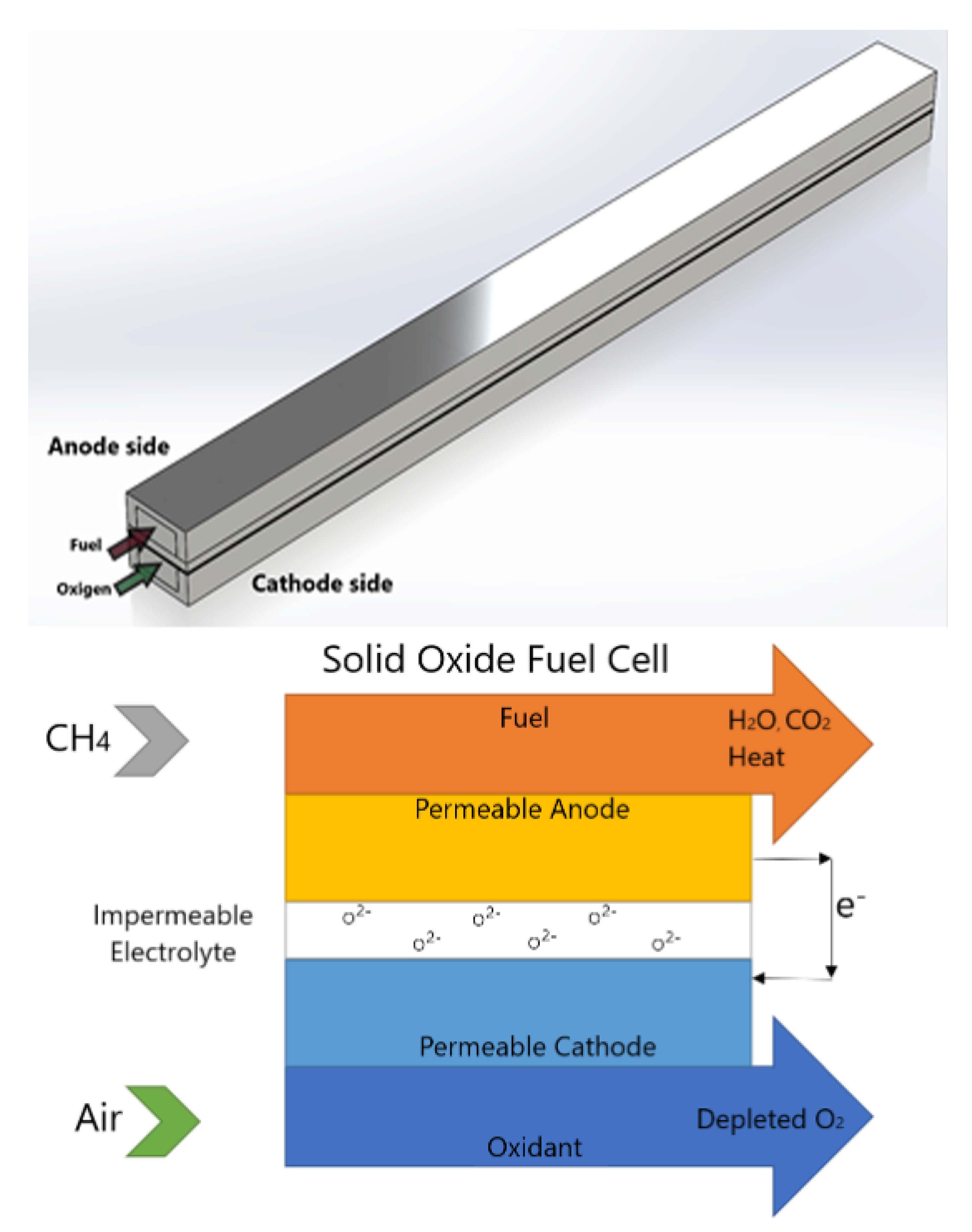
One of the electrochemical transformation gadgets that generate power straightforwardly from oxidizing a fuel is a Solid Oxide Fuel Cell (SOFC). The SOFC includes a solid oxide or ceramic electrolyte. Benefits of this type of fuel cells incorporate high joined warmth and power productivity, fuel adaptability, low emanations, and somewhat minimal expense. The biggest hindrance is the high working temperature which brings about longer beginning up occasions and mechanical and chemical adaptability similarity issues [54]. Figure 2 shows a schematic of SOFC and its reactions. SOFCs comprise numerous parts that each have their failure modes. The main part of this fuel cell is the anode. This section fostered the FMEA strategy for ceramic anodes. Figure 3 represented the most notable failure modes based on the Ishikawa fishbone diagram [55]. As it is obvious in literature, the main failure modes are considered: Interfacial delamination, Coke deposition, Sulfur adsorption onto the metal catalyst, Reduction in catalyst porosity, Corrosion of anode, and Crack. The offered process in this study is simultaneously the investigation of SOD factors and weight of criteria in a fully fuzzy environment and ultimately obtaining the rank of proposed failure modes.

Based on the previous mention, this work utilizes the FF-BWM method to weigh the factors. In this study, multiple DM methodology is used namely, three decision-makers give their ideas.

Table 4. Decision-makers ideas about risk factors.

BO Vector of Triple Factors					OW Vector of Triple Factors
	Best	S	O	D	Worst	S	O	D
DM1	S	JE	WS	SS	D	SS	ES	JE
DM2	S	JS	SS	VS	D	VS	WS	JE
DM3	O	ES	JE	WS	D	ES	WS	JE

includes these opinions.

Now according to Table 1 and Table 4, the FF-BWM mathematical model for the calculations of the mentioned model according to DM1 is presented below: The set of Other criteria to the Worst criterion (OW) and the set of the Best criterion to the Other criteria (BO) are obtained as follows:

$${\tilde{A}}_B=[(1,1,1),(1,3,5),(3,5,7)]$$

$${\tilde{A}}_W=[(3,5,7),(1,1,3),(1,1,1)]$$

The SODs weights based on TFNs, using Equations (20) to (31), will be as follows:

$$\mathrm{Min}\left({\theta }^1-\frac{1}{4}{\theta }^2+\frac{1}{4}{\theta }^3\right)$$

s.to:

$$w_S^1-\frac{1}{4}{w}_S^2+\frac{1}{4}{w}_S^3-((1+\frac{1}{4}(5-3))w_O^1-\frac{1}{4}\left(1\right)w_O^1+\frac{1}{4}\left(1\right)w_O^3)\le {\theta }^1-\frac{1}{4}{\theta }^2+\frac{1}{4}{\theta }^3$$

$$w_S^1-\frac{1}{4}{w}_S^2+\frac{1}{4}{w}_S^3-((1+\frac{1}{4}(5-3))w_O^1-\frac{1}{4}\left(1\right)w_O^1+\frac{1}{4}\left(1\right)w_O^3)\ge -\left({\theta }^1-\frac{1}{4}{\theta }^2+\frac{1}{4}{\theta }^3\right)$$

$$w_S^1-\frac{1}{4}{w}_S^2+\frac{1}{4}{w}_S^3-((3+\frac{1}{4}(7-5))w_D^1-\frac{1}{4}\left(3\right)w_D^1+\frac{1}{4}\left(3\right)w_D^3)\le {\theta }^1-\frac{1}{4}{\theta }^2+\frac{1}{4}{\theta }^3$$

$$w_S^1-\frac{1}{4}{w}_S^2+\frac{1}{4}{w}_S^3-((3+\frac{1}{4}(7-5))w_D^1-\frac{1}{4}\left(3\right)w_D^1+\frac{1}{4}\left(3\right)w_D^3)\ge -\left({\theta }^1-\frac{1}{4}{\theta }^2+\frac{1}{4}{\theta }^3\right)$$

$$w_O^1-\frac{1}{4}{w}_O^2+\frac{1}{4}{w}_O^3-((1+\frac{1}{4}(3-1))w_D^1-\frac{1}{4}\left(1\right)w_D^1+\frac{1}{4}\left(1\right)w_D^3)\le {\theta }^1-\frac{1}{4}{\theta }^2+\frac{1}{4}{\theta }^3$$

$$w_O^1-\frac{1}{4}{w}_O^2+\frac{1}{4}{w}_O^3-((1+\frac{1}{4}(3-1))w_D^1-\frac{1}{4}\left(1\right)w_D^1+\frac{1}{4}\left(1\right)w_D^3)\ge -\left({\theta }^1-\frac{1}{4}{\theta }^2+\frac{1}{4}{\theta }^3\right)$$

$$w_S^1-\frac{1}{4}{w}_S^2+\frac{1}{4}{w}_S^3+w_O^1-\frac{1}{4}{w}_O^2+\frac{1}{4}{w}_O^3+w_D^1-\frac{1}{4}{w}_D^2+\frac{1}{4}{w}_D^3=1$$

$$w_S^1-\frac{1}{4}{w}_S^2+\frac{1}{4}{w}_S^3\ge 0,w_O^1-\frac{1}{4}{w}_O^2+\frac{1}{4}{w}_O^3\ge 0,w_D^1-\frac{1}{4}{w}_D^2+1/4w_D^3\ge 0$$

$${\theta }^1-\frac{1}{4}{\theta }^2+\frac{1}{4}{\theta }^3\ge 0,{\theta }^2-{\theta }^1\ge 0,{\theta }^3-{\theta }^2\ge 0$$

$$w_S^2-w_S^1\ge 0,w_S^3-w_S^2\ge 0,w_O^2-w_O^1\ge 0,w_O^3-w_O^2\ge 0,w_D^2-w_D^1\ge 0,w_D^3-w_D^2\ge 0$$

Solving the above-mentioned correlations, the optimal final weights for SOD factors can be achieved:

• $w_S^{\ast }=(0.524,0.524,0.524),w_O^{\ast }=(0.309,0.309,0.309),$
• $w_D^{\ast }=(0.167,0.167,0.167),{\theta }^{\ast }=(0.059,0.059,0.059),$ CI factor will be $\frac{0.059}{11.27}=0.0055$ that $0.005<0.1$, so the results are acceptable.

Similarly, the triple factors’ ultimate optimal weight for all experts is presented in

Table 5. The optimal weights of triple factors.

DM	S			O			D
	1	2	3	1	2	3	1	2	3	θ*	CR
1	0.524	0.524	0.524	0.309	0.309	0.309	0.167	0.167	0.167	0.059	0.005
2	0.682	0.682	0.682	0.193	0.193	0.193	0.125	0.125	0.125	0.057	0.004
3	0.304	0.304	0.304	0.571	0.571	0.571	0.125	0.125	0.125	0.116	0.008

.

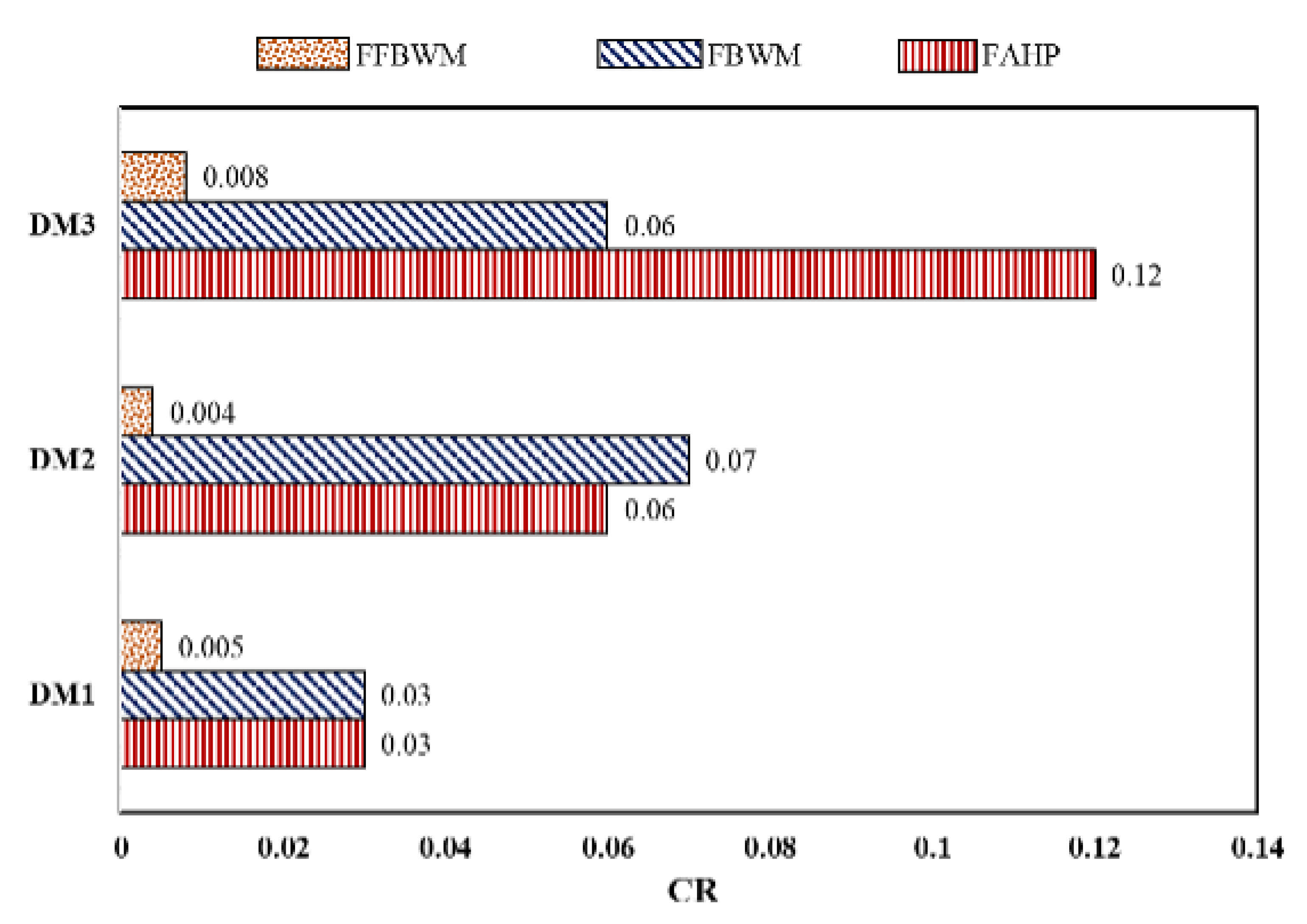
Table 5 represents the SOD factors optimal weights considering the optimal value of the objective function and CR factor that it is found that the results are acceptable. Herein, to show the reliability of the proposed approach in comparison to other weighting methods, the achieved CR factors are compared with those of F-BWM and F-AHP. Figure 3 compares CR factors For the three mentioned methodologies. In this Figure, CRs are presented based on separate DMs for each method. For instance, based on pairwise comparisons of DM1, F-BWM, and F-AHP are 0.03 while this value for FF-BWM is 0.005. This shows that pairwise comparisons of the proposed approach are more reliable and have higher consistency. According to this figure, pairwise comparisons of DM2 and DM3 have a similar condition.

Based on the mentioned issues, six main failure modes are considered in this study.

Table 6. Failure modes, causes, and effects.

No.	Failure Mode	Failure Cause	Results
FM1	Interfacial delamination	Re-oxidation reaction that causes volume change in anode	Conductivity reduction, voltage loss, system shutdown
FM2	Coke deposition	Non-complete oxidation (No shift reaction)	Conductivity reduction, voltage loss
FM3	Sulfur adsorption onto the metal catalyst	Fuel includes sulfur impurities	Voltage drop and productivity depreciation
FM4	Reduction in catalyst porosity	Red-ox reaction	Conductivity reduction, voltage loss
FM5	Corrosion of anode	Non-pure water, humidity exposure, corrosive atmosphere	Voltage reduction
FM6	Crack	Current overload	Drop-in voltage

shows all these failure modes and their circumstances and end results.

In the next step, failure modes scores are required. These scores are gathered in

Table 7. Failure modes scores based on SOD factors.

	S	O	D
FM1	9	2	9
FM2	5	5	5
FM3	5	5	5
FM4	5	6	5
FM5	3	4	4
FM6	9	6	6

.

Then,

Table 8. Assessments of failure modes concerning risk factors evaluated by the DM team.

Triple Factors	S			O			D
Failure Modes	${\mathit{DM}}^{\mathbf{1}}$	${\mathit{DM}}^{\mathbf{2}}$	${\mathit{DM}}^{\mathbf{3}}$	${\mathit{DM}}^{\mathbf{1}}$	${\mathit{DM}}^{\mathbf{2}}$	${\mathit{DM}}^{\mathbf{3}}$	${\mathit{DM}}^{\mathbf{1}}$	${\mathit{DM}}^{\mathbf{2}}$	${\mathit{DM}}^{\mathbf{3}}$
FM1	SS	S	S	W	W	SW	S	S	VS
FM2	F	F	F	F	F	SW	F	SW	SW
FM3	F	SS	SW	F	SW	SS	F	SS	SS
FM4	SS	F	F	F	F	SS	F	F	SW
FM5	SW	W	SW	SW	SW	SW	SW	SW	SW
FM6	VS	SS	SS	SS	SS	SS	SS	SS	F

consists of assessments of failure modes concerning risk factors evaluated by the DM team. These data are essential for failure modes ranking in fuzzy WASPAS.

Table 9. Converted group decision matrix to TFNs.

S			O			D
1	2	3	1	2	3	1	2	3
6.333	8.333	9.667	0.333	1.667	3.667	7.667	9.333	10.000
3.000	5.000	7.000	2.333	4.333	6.333	1.667	3.667	5.667
3.000	5.000	7.000	3.000	5.000	7.000	4.333	6.333	8.333
3.667	5.667	7.667	3.667	5.667	7.667	2.333	4.333	6.333
0.667	2.333	4.333	1.000	3.000	5.000	1.000	3.000	5.000
6.333	8.000	9.333	5.000	7.000	9.000	4.333	6.333	8.333

,

Table 10. WSM decision matrix.

S			O			D
1	2	3	1	2	3	1	2	3
0.330	0.434	0.503	0.013	0.066	0.146	0.107	0.130	0.139
0.156	0.260	0.364	0.093	0.172	0.252	0.023	0.051	0.079
0.156	0.260	0.364	0.119	0.199	0.278	0.060	0.088	0.116
0.191	0.295	0.399	0.146	0.225	0.305	0.032	0.060	0.088
0.035	0.121	0.226	0.040	0.119	0.199	0.014	0.042	0.070
0.330	0.417	0.486	0.199	0.278	0.358	0.060	0.088	0.116

and

Table 11. WPM decision matrix.

S			O			D
1	2	3	1	2	3	1	2	3
0.808	0.928	1.000	0.308	0.547	0.725	0.964	0.990	1.000
0.555	0.718	0.850	0.617	0.770	0.882	0.780	0.870	0.924
0.555	0.718	0.850	0.675	0.810	0.914	0.890	0.938	0.975
0.614	0.764	0.890	0.725	0.847	0.944	0.817	0.890	0.938
0.260	0.489	0.668	0.456	0.675	0.810	0.726	0.846	0.908
0.808	0.909	0.982	0.810	0.914	1.000	0.890	0.938	0.975

are the converted group decision matrix to TFNs, WSM, and WPM, respectively.

Ultimately, the final rank of failure modes can be achieved.

Table 12. SOFC failures modes prioritization.

Failure Mode		Conventional FMEA		Fuzzy WASPAS $\mathit{\alpha }=0.489$
		Traditional RPN	Rank	${\mathit{q}}_{\mathit{i}}$	${\mathit{p}}_{\mathit{i}}$	${\mathit{F}}_{\mathit{i}}$	Rank
FM1	Interfacial delamination	162	2	0.623	0.489	0.554	3
FM2	Coke deposition	125	4	0.484	0.480	0.482	5
FM3	Sulfur adsorption onto metal catalyst	125	4	0.547	0.546	0.546	4
FM4	Reduction in catalyst porosity	150	3	0.58	0.576	0.578	2
FM5	Corrosion of anode	48	5	0.288	0.286	0.287	6
FM6	Crack	324	1	0.777	0.774	0.775	1

shows the final failures modes prioritization using of Risk Priority Number (RPN). As it is clear, traditional RPN can not give a complete rank but fuzzy WASPAS is able to extract acceptable complete rank for considered failure modes.

Table 12 represents, as indicated by the Traditional RPN, failure mode FM2 and FM 3 with RPN = 125 has been situated in the fourth rank. Investigation of failure ranking dependent on the conventional RPN represented that during the time spent failure ranking, failures are assembled into five classifications. This shows that the ranking because of this conventional RPN doesn’t completely prioritize the failure modes and confuses the DM in risk management. As indicated by the examinations made in Table 12, the non-complete ranking of the failure modes may be because of avoiding the weight of SOD factors.

Contrasting the aftereffects of the fuzzy WASPAS rank and the traditional one represented that the full class rating of failure modes has been performed and failures that have been situated in a similar rank dependent on the traditional RPN are isolated into six classes dependent on the suggested approach. A considerable point is that FM1 and FM4 with the second and third ranks, respectively, in traditional RPN ranking, changes its rank to the third and second. Also, it can be found that FM6 namely Crack is the most important failure mode, and FM5, namely Corrosion of anode, is the least important one.

As Figure 3 mentions that the proposed approach is more reliable and accurate, herein, the effect of approach selection in final ranking for failure modes has been gathered in

Table 13. Failure modes rank comparison for all mentioned methods.

		F-WASPAS
Failure Mode		F-AHP	F-BWM	FF-BWM
		Rank
FM1	Interfacial delamination	20.623	20.489	3
FM2	Coke deposition	50.484	50.48	5
FM3	Sulfur adsorption onto metal catalyst	30.547	40.546	4
FM4	Reduction in catalyst porosity	40.58	30.576	2
FM5	Corrosion of anode	60.288	60.286	6
FM6	Crack	10.777	10.774	1

. This Table shows that failure modes rank by proposed methodology is different from two other methods and of course is closer to reality and includes decision makers’ preferences.

Triple factor sensitivity is analyzed by varying the weight of them based on the data given in

Table 14. Studied cases for sensitivity analysis.

	${\mathbf{Case}}^0$	${\mathbf{Case}}^1$	${\mathbf{Case}}^2$	${\mathbf{Case}}^3$	${\mathbf{Case}}^4$	${\mathbf{Case}}^5$	${\mathbf{Case}}^6$	${\mathbf{Case}}^7$
S	0.503	0.403	0.553	0.553	0.4	0.35	0.195	0.196
O	0.358	0.408	0.258	0.408	0.5	0.57	0.195	0.196
D	0.139	0.189	0.189	0.039	0.1	0.08	0.61	0.608

. In this table, eight cases are studied. ${\mathrm{Case}}^0$ shows the extracted weight values of the triple factors in the FF-BWM weighting process while the other cases represent distinctive weights for conceivable situations. The outcomes for positioning the failure modes for various cases are addressed in

Table 15. Final ranks of studied cases for sensitivity analysis.

	${\mathbf{Case}}^0$	${\mathbf{Case}}^1$	${\mathbf{Case}}^2$	${\mathbf{Case}}^3$	${\mathbf{Case}}^4$	${\mathbf{Case}}^5$	${\mathbf{Case}}^6$	${\mathbf{Case}}^7$
FM1	3	4	2	4	5	5	1	1
FM2	5	5	5	5	4	4	5	4
FM3	4	3	4	3	3	3	3	2
FM4	2	2	3	2	2	2	4	3
FM5	6	6	6	6	6	6	6	5
FM6	1	1	1	1	1	1	2	1

and Figure 4.

Based on Table 15, FM6 always comes in the first rank, but when the D factor has been increased by 4.38 times in ${\mathrm{Case}}^6$, the rank varies to second. Also, ${\mathrm{Case}}^7$ demonstrates that when the weight of D is 0.608 and the weights of S and O are 0.196, the approach will not represent complete rank, and FM1 and FM6 will both have the same rank.

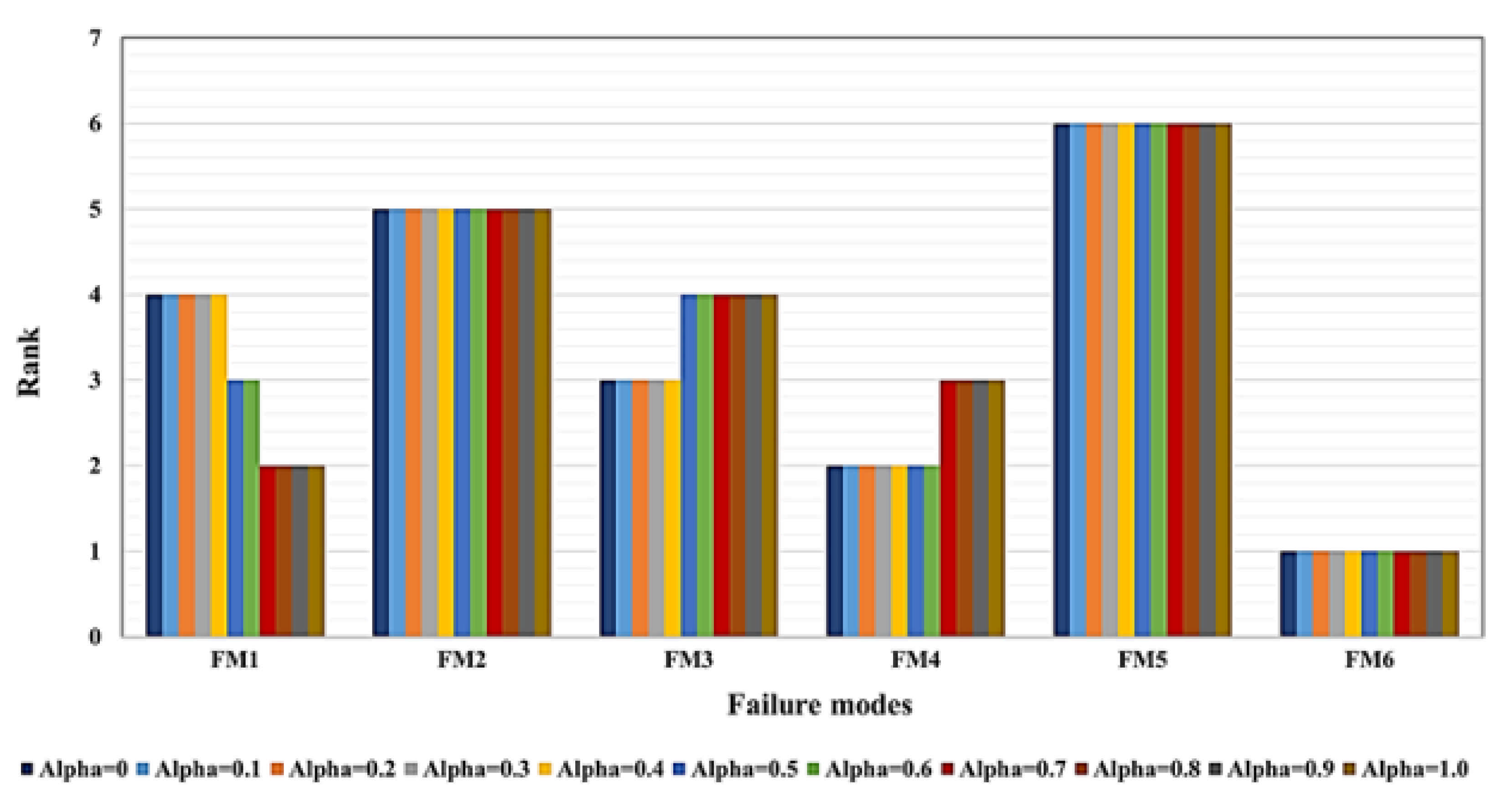
Depends on Figure 5, by varying variable $\alpha$ (UFC) from 0.0 to 1.0, FM2, FM5, and FM6 reserve their position in the ranking, but FM1, FM3, and FM4 change their situations. In considered UFC $(\alpha =0.489)$, the failure modes ranking is FM6 > FM4 > FM1 > FM3 > FM2 > FM5, while a change of $\alpha$ can vary this ranking as shown in Figure 5.

5. Conclusions

In this investigation, the main failure modes of a solid oxide fuel cell have been evaluated based on FMEA. The methodology consists of fully fuzzy BWM and fuzzy WASPAS. The uncertain risk assessment information is expressed by the fuzzy set-based method. To achieve the risk factors weights, the fully fuzzy BWM is employed. Then, the fuzzy WASPAS method is utilized to rank the failure modes. The results of the proposed approach based on the CR factor show that this method is more reliable and accurate than other methods like F-BWM and F-AHP. The final rank for considered failure modes shows that the achieved results in newly developed methodology is different from the other methods and based on having higher consistency is closer to reality. According to the obtained rank, crack (FM6) and reduction in catalyst porosity (FM4) are came in first and second rank, respectively, which means these failures should be considered by solid oxide fuel cell designers. Ultimately, sensitivity analyses are further extracted firstly by triple factors’ weight changing in seven cases and secondly by alpha changing from 0.0 to 1.0 with unit step. The results of this section show that the final rank is more dependent on alpha rather than triple factors’ weight. So, DM can use these results to choose suitable strategies among total existence strategies.

Some recommendations can be represented as follows. A hybrid system including spherical fuzzy sets, linguistics Z-number in the MCDM area, and interval type 2 fuzzy sets can be employed in various sciences such as economics, social issues, agriculture, energy systems, and so forth. Additionally, instead of FWASPAS, other ranking techniques like MOORA and VIKOR and also other MCDM methods such as SWARA can be utilized.

References

1. Mantelli, L.; De Campo, M.; Ferrari, M.; Magistri, L. Fuel flexibility for a turbocharged SOFC system. Energy Procedia 2019, 158, 1974–1979. [Google Scholar] [CrossRef]
2. Pashaee Golmarz, T.; Rezazadeh, S.; Bagherzadeh, N. Numerical study of curved-shape channel effect on performance and distribution of species in a proton-exchange membrane fuel cell: Novel structure. J. Renew. Energy Environ. 2018, 5, 10–21. [Google Scholar]
3. Pashaee Golmarz, T.; Rezazadeh, S.; Yaldagard, M.; Bagherzadeh, N. The Effect of Proton-Exchange Membrane Fuel Cell Configuration Changing from Straight to Cylindrical State on Performance and Mass Transport: Numerical Procedure. J. Renew. Energy Environ. 2021, 8, 39–53. [Google Scholar]
4. Besra, L.; Zha, S.; Liu, M. Preparation of NiO-YSZ/YSZ bi-layers for solid oxide fuel cells by electrophoretic deposition. J. Power Sources 2006, 160, 207–214. [Google Scholar] [CrossRef]
5. Guk, E.; Ranaweera, M.; Venkatesan, V.; Kim, J.S.; Jung, W. In-situ temperature monitoring directly from cathode surface of an operating solid oxide fuel cell. Appl. Energy 2020, 280, 116013. [Google Scholar] [CrossRef]
6. Gallo, M.; Polverino, P.; Mougin, J.; Morel, B.; Pianese, C. Coupling electrochemical impedance spectroscopy and model-based aging estimation for solid oxide fuel cell stacks lifetime prediction. Appl. Energy 2020, 279, 115718. [Google Scholar] [CrossRef]
7. Kong, W.; Han, Z.; Lu, S.; Ni, M. A simple but effective design to enhance the performance and durability of direct carbon solid oxide fuel cells. Appl. Energy 2021, 287, 116586. [Google Scholar] [CrossRef]
8. Xu, Q.; Xia, L.; He, Q.; Guo, Z.; Ni, M. Thermo-electrochemical modelling of high temperature methanol-fuelled solid oxide fuel cells. Appl. Energy 2021, 291, 116832. [Google Scholar] [CrossRef]
9. Wang, C.; Liao, M.; Liang, B.; Jiang, Z.; Zhong, W.; Chen, Y.; Luo, X.; Shu, R.; Tian, Z.; Lei, L. Enhancement effect of catalyst support on indirect hydrogen production from propane partial oxidation towards commercial solid oxide fuel cell (SOFC) applications. Appl. Energy 2021, 288, 116362. [Google Scholar] [CrossRef]
10. Zaghloul, M.A.; Mason, J.H.; Wang, M.; Buric, M.; Peng, Z.; Lee, S.; Ohodnicki, P.; Abernathy, H.; Chen, K.P. High spatial resolution temperature profile measurements of solid-oxide fuel cells. Appl. Energy 2021, 288, 116633. [Google Scholar] [CrossRef]
11. Singh, P.; Meena, N.K.; Yang, J.; Vega-Fuentes, E.; Bishnoi, S.K. Multi-criteria decision making monarch butterfly optimization for optimal distributed energy resources mix in distribution networks. Appl. Energy 2020, 278, 115723. [Google Scholar] [CrossRef]
12. Saaty, R.W. The analytic hierarchy process—What it is and how it is used. Math. Model. 1987, 9, 161–176. [Google Scholar] [CrossRef] [Green Version]
13. Saaty, T.L. Theory and Applications of the Analytic Network Process: Decision Making with Benefits, Opportunities, Costs, and Risks; RWS Publications: Pittsburgh, PA, USA, 2005. [Google Scholar]
14. Keršuliene, V.; Zavadskas, E.K.; Turskis, Z. Selection of rational dispute resolution method by applying new step-wise weight assessment ratio analysis (SWARA). J. Bus. Econ. Manag. 2010, 11, 243–258. [Google Scholar] [CrossRef]
15. Rezaei, J. Best-worst multi-criteria decision-making method. Omega 2015, 53, 49–57. [Google Scholar] [CrossRef]
16. Pamučar, D.; Stević, Ž.; Sremac, S. A new model for determining weight coefficients of criteria in mcdm models: Full consistency method (fucom). Symmetry 2018, 10, 393. [Google Scholar] [CrossRef] [Green Version]
17. Haseli, G.; Sheikh, R.; Sana, S.S. Base-criterion on multi-criteria decision-making method and its applications. Int. J. Manag. Sci. Eng. Manag. 2020, 15, 79–88. [Google Scholar] [CrossRef]
18. Hwang, C.L.; Yoon, K. Methods for multiple attribute decision making. In Multiple Attribute Decision Making; Springer: Berlin/Heidelberg, Germany, 1981; pp. 58–191. [Google Scholar]
19. Opricovic, S. Multicriteria optimization of civil engineering systems. Fac. Civ. Eng. Belgrade 1998, 2, 5–21. [Google Scholar]
20. Brauers, W.K.; Zavadskas, E.K. The MOORA method and its application to privatization in a transition economy. Control. Cybern. 2006, 35, 445–469. [Google Scholar]
21. Zavadskas, E.K.; Kaklauskas, A.; Turskis, Z.; Tamošaitiene, J. Selection of the effective dwelling house walls by applying attributes values determined at intervals. J. Civ. Eng. Manag. 2008, 14, 85–93. [Google Scholar] [CrossRef] [Green Version]
22. Zavadskas, E.K.; Turskis, Z.; Antucheviciene, J.; Zakarevicius, A. Optimization of weighted aggregated sum product assessment. Elektron. Elektrotechnika 2012, 122, 3–6. [Google Scholar] [CrossRef]
23. Yazdani, M.; Zarate, P.; Zavadskas, E.K.; Turskis, Z. A Combined Compromise Solution (CoCoSo) method for multi-criteria decision-making problems. Manag. Decis. 2019, 57, 2501–2519. [Google Scholar] [CrossRef]
24. Ju-Long, D. Control problems of grey systems. Syst. Control Lett. 1982, 1, 288–294. [Google Scholar] [CrossRef]
25. Kuo, M.S.; Liang, G.S. Combining VIKOR with GRA techniques to evaluate service quality of airports under fuzzy environment. Expert Syst. Appl. 2011, 38, 1304–1312. [Google Scholar] [CrossRef]
26. Turskis, Z.; Zavadskas, E.K.; Antucheviciene, J.; Kosareva, N. A hybrid model based on fuzzy AHP and fuzzy WASPAS for construction site selection. Int. J. Comput. Commun. Control 2015, 10, 113–128. [Google Scholar] [CrossRef]
27. Gupta, H.; Barua, M.K. A framework to overcome barriers to green innovation in SMEs using BWM and Fuzzy TOPSIS. Sci. Total. Environ. 2018, 633, 122–139. [Google Scholar] [CrossRef] [PubMed]
28. Rahimi, S.; Hafezalkotob, A.; Monavari, S.M.; Hafezalkotob, A.; Rahimi, R. Sustainable landfill site selection for municipal solid waste based on a hybrid decision-making approach: Fuzzy group BWM-MULTIMOORA-GIS. J. Clean. Prod. 2020, 248, 119186. [Google Scholar] [CrossRef]
29. Celik, E.; Gul, M. Hazard identification, risk assessment and control for dam construction safety using an integrated BWM and MARCOS approach under interval type-2 fuzzy sets environment. Autom. Constr. 2021, 127, 103699. [Google Scholar] [CrossRef]
30. Ghoushchi, S.J.; Dorosti, S.; Khazaeili, M.; Mardani, A. Extended approach by using best–worst method on the basis of importance–necessity concept and its application. Appl. Intell. 2021, 9, 1–15. [Google Scholar]
31. Zavadskas, E.K.; Antucheviciene, J.; Hajiagha, S.H.R.; Hashemi, S.S. Extension of weighted aggregated sum product assessment with interval-valued intuitionistic fuzzy numbers (WASPAS-IVIF). Appl. Soft Comput. 2014, 24, 1013–1021. [Google Scholar] [CrossRef]
32. Kutlu Gundogdu, F.; Kahraman, C. Extension of WASPAS with spherical fuzzy sets. Informatica 2019, 30, 269–292. [Google Scholar] [CrossRef] [Green Version]
33. Rudnik, K.; Bocewicz, G.; Kucińska-Landwójtowicz, A.; Czabak-Górska, I.D. Ordered fuzzy WASPAS method for selection of improvement projects. Expert Syst. Appl. 2021, 169, 114471. [Google Scholar] [CrossRef]
34. Haseli, G.; Sheikh, R.; Sana, S.S. Extension of base-criterion method based on fuzzy set theory. Int. J. Appl. Comput. Math. 2020, 6, 1–24. [Google Scholar] [CrossRef]
35. Rezaei, J. Best-worst multi-criteria decision-making method: Some properties and a linear model. Omega 2016, 64, 126–130. [Google Scholar] [CrossRef]
36. Mou, Q.; Xu, Z.; Liao, H. An intuitionistic fuzzy multiplicative best-worst method for multi-criteria group decision making. Inf. Sci. 2016, 374, 224–239. [Google Scholar] [CrossRef]
37. Guo, S.; Zhao, H. Fuzzy best-worst multi-criteria decision-making method and its applications. Knowl.-Based Syst. 2017, 121, 23–31. [Google Scholar] [CrossRef]
38. Aboutorab, H.; Saberi, M.; Asadabadi, M.R.; Hussain, O.; Chang, E. ZBWM: The Z-number extension of Best Worst Method and its application for supplier development. Expert Syst. Appl. 2018, 107, 115–125. [Google Scholar] [CrossRef]
39. Ghoushchi, S.J.; Yousefi, S.; Khazaeili, M. An extended FMEA approach based on the Z-MOORA and fuzzy BWM for prioritization of failures. Appl. Soft Comput. 2019, 81, 105505. [Google Scholar] [CrossRef]
40. Liu, A.; Ji, X.; Lu, H.; Liu, H. The selection of 3PRLs on self-service mobile recycling machine: Interval-valued pythagorean hesitant fuzzy best-worst multi-criteria group decision-making. J. Clean. Prod. 2019, 230, 734–750. [Google Scholar] [CrossRef]
41. Akbari, R.; Dabbagh, R.; Ghoushchi, S.J. HSE risk prioritization of molybdenum operation process using extended FMEA approach based on Fuzzy BWM and Z-WASPAS. J. Intell. Fuzzy Syst. 2020, 38, 5157–5173. [Google Scholar] [CrossRef]
42. Mohammadi, M.; Rezaei, J. Bayesian best-worst method: A probabilistic group decision making model. Omega 2020, 96, 102075. [Google Scholar] [CrossRef]
43. Mei, M.; Chen, Z. Evaluation and selection of sustainable hydrogen production technology with hybrid uncertain sustainability indicators based on rough-fuzzy BWM-DEA. Renew. Energy 2021, 165, 716–730. [Google Scholar] [CrossRef]
44. Amiri, M.; Hashemi-Tabatabaei, M.; Ghahremanloo, M.; Keshavarz-Ghorabaee, M.; Zavadskas, E.K.; Antucheviciene, J. A novel model for multi-criteria assessment based on BWM and possibilistic chance-constrained programming. Comput. Ind. Eng. 2021, 156, 107287. [Google Scholar] [CrossRef]
45. Pamučar, D.; Puška, A.; Stević, Ž.; Ćirović, G. A new intelligent MCDM model for HCW management: The integrated BWM–MABAC model based on D numbers. Expert Syst. Appl. 2021, 175, 114862. [Google Scholar] [CrossRef]
46. Mohtashami, A. A novel modified fuzzy best-worst multi-criteria decision-making method. Expert Syst. Appl. 2021, 181, 115196. [Google Scholar] [CrossRef]
47. Haseli, G.; Sheikh, R.; Wang, J.; Tomaskova, H.; Tirkolaee, E.B. A Novel Approach for Group Decision Making Based on the Best–Worst Method (G-BWM): Application to Supply Chain Management. Mathematics 2021, 9, 1881. [Google Scholar] [CrossRef]
48. Karimi, H.; Sadeghi-Dastaki, M.; Javan, M. A fully fuzzy best–worst multi attribute decision making method with triangular fuzzy number: A case study of maintenance assessment in the hospitals. Appl. Soft Comput. 2020, 86, 105882. [Google Scholar] [CrossRef]
49. Zadeh, L.A.; Klir, G.J.; Yuan, B. Fuzzy Sets, Fuzzy Logic, and Fuzzy Systems: Selected Papers; World Scientific: Singapore, 1996; Volume 6, pp. 394–432. [Google Scholar]
50. Chang, D.Y. Applications of the extent analysis method on fuzzy AHP. Eur. J. Oper. Res. 1996, 95, 649–655. [Google Scholar] [CrossRef]
51. Kaufmann, A.; Gupta, M.M. Fuzzy Mathematical Models in Engineering and Management Science; Elsevier Science Inc.: New York, NY, USA, 1988. [Google Scholar]
52. Allahviranloo, T.; Lotfi, F.H.; Kiasary, M.K.; Kiani, N.; Alizadeh, L. Solving fully fuzzy linear programming problem by the ranking function. Appl. Math. Sci. 2008, 2, 19–32. [Google Scholar]
53. Easton, A. One-of-a-kind decisions involving weighted multiple objectives and disparate alternatives. Mult. Criteria Decis. Mak. 1973, 657–667. [Google Scholar]
54. Badwal, S.; Giddey, S.; Munnings, C.; Kulkarni, A. Review of progress in high temperature solid oxide fuel cells. ChemInform 2014, 46, 23–37. [Google Scholar]
55. Patel, N.K.; Bishop, S.R.; Utter, R.G.; Das, D.; Pecht, M. Failure modes, mechanisms, effects, and criticality analysis of ceramic anodes of solid oxide fuel cells. Electronics 2018, 7, 323. [Google Scholar] [CrossRef] [Green Version]
Figure 1. Offered approach flow chart.
Mathematics 09 02328 g001
Figure 2. SOFC schematic and its reaction.
Mathematics 09 02328 g002
Figure 3. Comparison of CR factors for the three mentioned methodologies.
Mathematics 09 02328 g003
Figure 4. Sensitivity analysis for studied case studies with constant α .
Mathematics 09 02328 g004
Figure 5. Sensitivity analysis for studied case studies with variable α (UFC).
Mathematics 09 02328 g005