Between Scylla and Charybdis: The Bermudan Swaptions Pricing Odyssey

Abstract

Bermudan swaptions are options on interest rate swaps which can be exercised on one or more dates before the final maturity of the swap. Because the exercise boundary between the continuation area and stopping area is inherently complex and multi-dimensional for interest rate products, there is an inherent “tug of war” between the pursuit of calibration and pricing precision, tractability, and implementation efficiency. After reviewing the main ideas and implementation techniques underlying both single- and multi-factor models, we offer our own approach based on dimension reduction via Markovian projection. Specifically, on the theoretical side, we provide a reinterpretation and extension of the classic result due to Gyöngy which covers non-probabilistic, discounted, distributions relevant in option pricing. Thus, we show that for purposes of swaption pricing, a potentially complex and multidimensional process for the underlying swap rate can be collapsed to a one-dimensional one. The empirical contribution of the paper consists in demonstrating that even though we only match the marginal distributions of the two processes, Bermudan swaptions prices calculated using such an approach appear well-behaved and closely aligned to counterparts from more sophisticated models.

1. Outline

Interest rate contracts constitute the largest chunk of the global over-the-counter derivatives market, with an estimated total notional outstanding of just over $480 trillion, of which roughly $350 trillion is traded in swaps and almost $50 trillion is traded in interest rate options. The total market value of interest rate swaps and options tallied together exceeds $8 trillion—or about 10% of world GDP.

Anticipating a more formal discussion, an interest rate swap is simply a contract in which two parties exchange two flows of payments (“legs”)—one calculated on the basis of a fixed, pre-determined rate (coupon), and one calculated on the basis of a floating interest rate (typically the interbank market benchmark, often referred to as- London Interbank Offered Rate (LIBOR). Swap options, or swaptions, give the owner the right—but not the obligation—to enter into an interest rate swap with a given final maturity and a pre-determined strike rate at a certain, specific time in the future called option expiration and corresponding to the fixing date of the swap. Swaptions come in many shapes and forms, some more complex (“exotic”) than others. A prototypical example of an exotic interest rate derivative is a Bermudan swaption. Somewhat, the name has nothing to do with geography, but rather with the option exercise profile, as Bermudans, unlike their simpler—so-called European—counterparts, can be exercised not just on a single date, but on any one of a given set of dates prior to the final maturity of the swap (an option that can be exercised at any time is called American).

While we do not know exactly how much of the total market value of interest rate derivatives is made up by Bermudan swaptions, such a breakdown would not do full justice to their importance anyway, as the numbers cited do not account for options and option-like features of Bermudan nature built into simpler fixed income instruments, like callable bonds and mortgage backed securities. Consider that roughly 60% of bonds included in the Bloomberg Barclays Global Aggregate Credit Index—a widely followed benchmark for the corporate bond universe—are issued with call provisions giving issuers the right to repurchase them at par at certain dates in the future. The call provision may be added to increase the coupon, and hence the perceived attractiveness of the issue, but it rarely stays with the issuer, who will instead typically seek to strip the call option and sell it—e.g., in the form of a cancelable swap—to an exotic dealer desk to lower the effective cost of the issuance. For example, Goldman Sachs analysts estimate that Bermudans embedded in 70% of the so-called Formosa bonds (bonds that are denominated in a foreign currency, but registered and listed on the Taipei Exchange) acquire a new life being passed on to exotic dealer desks who tend to actively manage this risk by selling European swaptions with risks most closely mimicking that of the Bermudan (effectively providing “Vega supply” to the market) (“Formosa issuance and USD rate vol supply”, Global Rates Insight, Goldman Sachs, 13 February 2020). Other notable natural buyers of such stripped Bermudan swaptions are mortgage originators or issuers of mortgage-backed securities (such as, e.g., Fannie Mae and Freddie Mac in the US), who seek to offset the risk of prepayment options inherent in typical fixed rate mortgage products.

What is special about Bermudan swaptions, and what explains their important role in the financial system, is the complex risk profile stemming from the multiple exercise feature. It turns out that accounting properly for this exotic feature poses a considerable challenge and has been a major driver of the (r)evolution in interest rate modeling—a story that we intend to tell below.

From a mathematical standpoint, the early exercise property gives rise to a free boundary problem not unlike the so-called Stefan problem encountered when analyzing the temperature of water bordering a melting block of ice: if there are N exercise dates $T_1,T_2,\dots ,T_N$, then at each $T_i$, $i\in \{1,2,\dots ,N\}$, the Bermudan holder must decide whether to retain the option or exercise by entering into the i-th co-terminal swap. Naturally, for each $T_i$ there will be some critical value of the underlying instrument below which it no longer makes sense to exercise. This reduces the problem of valuing the Bermudan to determining the optimal exercise boundary that separates the “region” where exercise is optimal from the “region” where it is optimal to continue holding the swaption—with obvious analogies to Stefan problems for the location of the interface between water and melting ice (see, e.g., [1]). Such parallels have been known for decades and fruitfully exploited, at least in the case of early exercise boundaries for American-style equity options. And while an early exercise boundary as such cannot be solved for in closed form, it can be represented using an integral equation to be solved iteratively [2] and its upper and lower bounds can be rigorously determined. Barles, Burdeau, Romano, and Samsoen [3] even show that near expiration these upper and lower bounds approach each other, which leads them to postulate an approximation for the value of the option.

Unfortunately, those results do not carry through to interest rate options in a straightforward way. For one, the partial differential equation governing the evolution of the stock option price (the Black–Scholes Partial Differential Equation(PDE)) has been derived under the assumption that the underlying instrument, a share of common stock, is a tradable asset. After all, as shown by Black and Scholes [4], the self-financing dynamic trading strategy replicating the final payoff of the option is implemented by taking positions in, i.e., buying and selling, units of the underlying instrument. That underlying instrument may be—as initially considered—a stock or a commodity futures contract, but not an interest rate that is not tradable—one cannot “buy” or “sell” a yield on, say, a 10-year bond, a swap rate or the LIBOR. As it turns out, this obstacle can be overcome by a judicious application of the change-of-measure technique ([5]; more on this below). But even if one can come up with an equivalent probability measure under which a given underlying interest rate is a martingale, and thus price the option by simply taking expectation of the terminal payoff, a more profound problem arises: how to ensure consistency between options on different interest rate underlyings? The crucial difference between interest rates and, say, stocks—other than tradability—is that individual interest rates are simply pieces of a greater whole called the term structure, bound together by no-arbitrage relations and complex correlation patterns. This becomes immediately clear when we consider a swaption where the underlying is a (stochastic) average of a number of forward LIBOR rates. As explained above, a Bermudan can even be viewed as a “best of” chooser option to optimally select and enter into one of potentially many co-terminal swaps spanned by the contract. As such, it is by definition an instrument driven by complex dependence patterns among interest rate underlyings—a phenomenon we shall have more to say on later. All this implies that handling interest rate derivatives, and Bermudans especially, requires a consistent model of the term structure. And since different approaches have been proposed to the modeling of interest rates, so too there have been—and still are—different ideas about pricing and risk-managing Bermudan swaptions.

Although it is impossible within the confines of this essay to do justice to the large and still growing literature in the area of interest rate modeling ([6,7] and vol. II are very good general references), we may, at least at this stage, identify two broad schools of thought: low-factor short-rate models and multi-factor market models. The first camp, drawing inspiration from Vasicek [8], starts from a fundamental assumption that the dynamics of the whole yield curve is driven by the “instantaneous spot rate”, or short rate, $r\left(t\right)$, at which interest accrues continuously in a locally risk-free way. This definition leads to the so-called money market account, $B\left(t\right)$, which evolves according to:

$$dB\left(t\right)=r\left(t\right)B\left(t\right)dt,B\left(0\right)=1,$$

(1)

and induces the risk-neutral measure $\mathbb{Q}$ making all discounted asset prices martingales. Although the short rate is a purely artificial mathematical construct (all be it with an intuitive interpretation), it determines prices of all discount bond that are simply $\mathbb{Q}$-expectations of the future path of $r\left(t\right)$, ${\int }_t^{T}r\left(s\right)ds$. And since all interest rates are derived from bond prices, it follows that the entire discount curve can in principle be parameterized by stipulating a suitable stochastic process for $r\left(t\right)$—a point supported by a large body of empirical evidence suggesting that the first principal component typically accounts for about 90% of the variation in the entire term structure. With two factors—two state variables feeding through to the evolution of $r\left(t\right)$—one would expect to cover well over 95% of yield curve variation. Apart from parsimony and consistency, short rate models have another considerable virtue that came to explain their initial success as tools-of-choice for the valuation of path-dependent interest rate instruments such as Bermudan swaptions: they are relatively easy to implement numerically in lattices, i.e., finite differences or trees, which can efficiently handle the early exercise boundary through backward induction.

However, these virtues do not come without vices to match. With only one or two factors, it might be difficult to generate all practically relevant yield curve shapes (two Principal Components Analysis PCAs would still leave about 5% of variation unexplained) and match a large set of market prices—especially with intuitive and economically justifiable parameter values (using a large set of calibration instruments is necessary if one wishes to consistently apply a single calibrated model to many kinds of exotic interest rate derivatives). More importantly, a low number of factors (one or two) may limit the degree of de-correlation achievable among interest rates, artificially lowering prices of Bermudan swaptions (when correlation among rates is high, the right to choose among different swaptions is lower than in the case when interest rates are decorrelated and subsequent payoffs are unpredictable). Longstaff, Santa-Clara, and Schwartz [9] even thought that the errors and pitfalls of using single-factor models amounted to “throwing away a billion dollars” and in their influential paper argued for a move towards a multi-factor setting. In fact, the stage in that respect had already been set in the form of so-called LIBOR/swap market models [10,11,12] and their later extensions. Models in this class are generally expressed in terms of discretely compounded market rates (hence the term “market models”), each of which can be shown to be a martingale under an appropriate forward measure. This perspective naturally allows for multiple sources of randomness (often there are more than 50 state variables), with almost arbitrarily complex dependence structure, and offers many degrees of freedom to fit observed market patterns, even including the so-called implied volatility smiles (e.g., [13,14] or [15]; cf. also [16,17,18,19,20,21,22]). Whether the number of factors, in and of itself, is enough to improve the pricing of Bermudans has been persuasively contested [23] and we shall review the main arguments presented in this debate. It is clear, however, that while increasing dimensionality improves calibration, it does so at the cost of efficiency and numerical accuracy: with a high number of state variables, lattice techniques are no longer viable, and even if viable (cf. e.g., [24])—not really practicable. One therefore is left with Monte Carlo simulations (with some variance reduction technique to reduce bias). This presents an obvious problem: by evolving the underlying state variables forward in time, the simulation cannot easily determine the optimal time to exercise. And while efficient techniques of circumventing that problem have since been proposed (cf. especially the classic approach of [25,26] for a very good general reference), the exercise region and corresponding Bermudan swaption prices will necessarily be estimated—not exact.

The two approaches sketched broadly above, the single- and multi-factor ones, are like Scylla and Charybdis, the mythical sea monsters, lurking for the Bermudan swaption modeler: pass too close to Scylla, and your model shall crash against the rocks of computational challenges and estimation biases of the multidimensional setting; move towards Charybdis and risk getting sucked by a whirlpool of artificial parameter values and unachievable calibration targets. And yet, unlike in the classical Greek tragedy, we believe there is safe passage between the two hazards, and one that does not involve losing six strongest and bravest companions—a cost tragically borne by Odysseus. Thus, in what follows we try to tell the story—the odyssey—behind the evolution of Bermudan swaption pricing in greater detail, reviewing in a much more formal way the main ideas and solutions underlying both single- and multi-factor models. We discuss their relative merits and drawbacks, presenting especially the crux of the consensus-shattering debate between Longstaff, Santa-Clara, and Schwartz [9] and Andersen and Andreasen [23]. Finally, building on Gatarek and Jabłecki [27], we show our dimension reduction approach based on the concept of Markovian projection pioneered by Gyöngy [28] and independently adapted to the financial landscape by Dupire [29] under the guise of “local volatility”. Our idea consists essentially in showing that for purposes of pricing Bermudan swaptions, a potentially complex and multidimensional process for the swap rate can—using the tools of Markovian projection—be collapsed to a one-dimensional one. Naturally, the diffusions of the two processes will differ, but it turns out the early exercise boundaries will approximately agree, with pricing errors within normal bid–ask spreads.

The rest of the essay proceeds as follows. Section 2 presents notation and formally introduces the relevant interest rate instruments. Section 3 presents the evolution of term structure modeling, from single- to multi-factor approaches, zooming in on implementation and calibration aspects. Section 4 then discusses the specific challenges related to applying the models in the context of pricing Bermudan swaptions, and revisits the issue of their factor dependence with some numerical tests. Finally, Section 5 presents a novel argument in the factor-sensitivity debate, demonstrating an elegant extension of the classic result due to Gyöngy [28] on Markovian projection and dimension reduction. Section 6 draws conclusions.

2. Notation, Modeling Setting and Instruments

Consider a continuous-time economy together with a probability space $(\Omega ,\mathcal{F},\mathbb{P})$ with a frictionless and arbitrage-free market for zero coupon bonds, i.e., contracts that guarantee holders the payment of one unit of currency at maturity, with no intermediate payments. Let $P(t,T)$ be the time t price of a zero coupon bond maturing at time T such that $P(t,t)=1$ for every t. We assume that such a $P(t,T)$ exists for every $0<t<T<\infty$ and for a given t, $P(t,T)$ is differentiable with respect to maturity time T. The instantaneous forward rate $f(t,T)$ with maturity T contracted at t is defined by:

$$f(t,T)\equiv -\frac{\partial lnP(t,T)}{\partial T}\iff P(t,T)=exp\left(-{\int }_t^{T}f(t,s)ds\right).$$

(2)

The instantaneous spot rate $r\left(t\right)$—i.e., the short rate—has already been loosely defined above and can now be formalized as:

$$r\left(t\right)\equiv f(t,t).$$

(3)

As discussed, $r\left(t\right)$ can be thought of as capturing the locally risk-free return from a continuously compounded money market account $B\left(t\right)\equiv exp\left\{{\int }_0^{t}r\left(s\right)ds\right\}$ with dynamics $dB\left(t\right)=r\left(t\right)B\left(t\right)dt,B\left(0\right)=1$. The significance of the money market account in modern finance stems from the fact that it establishes a connection between the economic concept of absence of arbitrage and the mathematical property of existence of the equivalent martingale measure (risk-neutral measure). Specifically, as shown by Harrison and Kreps (1979) and Harrison and Pliska (1981, 1983), postulating that our market is arbitrage-free is equivalent to stating that there exists a measure $\mathbb{Q}$ on $(\Omega ,\mathcal{F})$, equivalent to $\mathbb{P}$, such that all asset prices discounted by $B\left(t\right)$ are $\mathbb{Q}$-martingales. In other words, in our economy, for any T we have:

$$\frac{P(0,T)}{B\left(0\right)}=P(0,T)={\mathbb{E}}^{\mathbb{Q}}\left(\frac{P(T,T)}{B\left(T\right)}\right)={\mathbb{E}}^{\mathbb{Q}}\left(\frac{1}{B\left(T\right)}\right)={\mathbb{E}}^{\mathbb{Q}}\left(exp\left\{-{\int }_0^{T}r\left(s\right)ds\right\}\right),$$

(4)

so that time-zero bond (asset) prices are $\mathbb{Q}$-expectations of their terminal values (payoffs). We will explore (4) in Section 3 in greater detail as it gives rise to an important class of term structure models, but for now let us simply observe that when we allow for stochastic interest rates—as we naturally should when dealing with interest rate derivatives—the martingale measure $\mathbb{Q}$ may not be the most convenient or natural to work with. Thus, Geman et al. (1995) prove that for any positive non-dividend-paying asset N (so-called numeraire) there exists a measure ${\mathbb{Q}}^N$, which is equivalent to the original martingale measure $\mathbb{Q}$, making the prices of all claims normalized by N ${\mathbb{Q}}^N$-martingales. Furthermore, the Radon–Nikodym derivative defining ${\mathbb{Q}}^N$ is given simply by $B\left(T\right)N\left(T\right)/N\left(0\right)$.

We now move on to introducing other instruments. For this we define a uniformly spaced tenor structure:

$$0=T_0<T_1<\dots <T_N,$$

(5)

and set ${\delta }_n=T_n-T_{n-1}$ for $n=1,\dots ,N$. A spot LIBOR rate over the interval $(T_{n-1},T_n)$ is given by the formula:

$$L(T_{n-1},T_n)=\frac{1-P(T_{n-1},T_n)}{{\delta }_{n}P(T_{n-1},T_n)}$$

(6)

whereas its forward counterpart, forward LIBOR, is given by:

$$F_n\left(t\right)=F(t,T_{n-1},T_n)=\frac{P(t,T_{n-1})-P(t,T_n)}{{\delta }_{n}P(t,T_n)}.$$

(7)

A fixed-for-floating interest rate swap (IRS) with unit notional, fixed rate (coupon) K, and a specified tenor structure $\mathcal{T}={\left\{T_n\right\}}_{n=\alpha +1}^{\beta }$ is a contract whereby two parties exchange differently indexed cashflows over a pre-agreed time span. Specifically, on each date $T_n\in \mathcal{T}$, the fixed leg pays ${\delta }_{n}K$, whereas the floating leg pays the floating LIBOR rate given by (6). When the fixed leg is paid, the IRS is called a “payer”, and conversely the swap is called a “receiver.”

An interest rate cap/floor is a payer (receiver) IRS in which each payment is executed only if it has positive value. It has become market practice to quote prices of caps in terms of Black’s implied volatilities, i.e., parameters ${\sigma }_{\alpha ,\beta }$, which plugged into the formula:

$$\sum _{i=\alpha +1}^{\beta }P(0,T_n){\delta }_n\left[F_n\left(0\right)\Phi \left(\frac{ln\left(\frac{F_n\left(0\right)}{K}\right)+\frac{1}{2}{\sigma }_{\alpha ,\beta }^2{T}_{n-1}}{{\sigma }_{\alpha ,\beta }\sqrt{T_{n-1}}}\right)-K\Phi \left(\frac{ln\left(\frac{F_n\left(0\right)}{K}\right)-\frac{1}{2}{\sigma }_{\alpha ,\beta }^2{T}_{n-1}}{{\sigma }_{\alpha ,\beta }\sqrt{T_{n-1}}}\right)\right]$$

(8)

give the market price. The Black model itself is inconsistent with market quotes, which tend to exhibit a pronounced implied volatility smile/skew.

The forward swap rate $S_{\alpha ,\beta }\left(t\right)$ corresponding to the tenor structure $\mathcal{T}$ is the rate in the fixed leg that sets it equal to the floating leg and hence makes the net present value of the transaction equal zero:

$$S_{\alpha ,\beta }\left(t\right)\equiv \frac{P(t,T_{\alpha })-P(t,T_{\beta })}{{\sum }_{n=\alpha +1}^{\beta }P(t,T_n){\delta }_n}.$$

(9)

The portfolio of zero-coupon bonds in the denominator of Equation (9) is the so-called annuity factor, for which we will sometimes use a continuous-time definition, writing $N_{\alpha ,\beta }\left(t\right)\equiv {\int }_{T_{\alpha }}^{T_{\beta }}P(t,u)du$ along with:

$$S_{\alpha ,\beta }\left(t\right)=\frac{P(t,T_{\alpha })-P(t,T_{\beta })}{N_{\alpha ,\beta }\left(t\right)}=\frac{{\int }_{T_{\alpha }}^{T_{\beta }}P(t,s)f(t,s)ds}{N_{\alpha ,\beta }\left(t\right)}.$$

(10)

Note, in passing, that since $N_{\alpha ,\beta }\left(t\right)$ is positive and $P(t,T_{\alpha })-P(t,T_{\beta })$ is a tradable asset (a portfolio of “long” the $T_{\alpha }$ bond and “short” the $T_{\beta }$ one), it follows that $S_{\alpha ,\beta }\left(t\right)$ is a martingale under ${\mathbb{Q}}^{\alpha ,\beta }$ induced by $N_{\alpha ,\beta }\left(t\right)$.

A European payer (receiver) swaption with strike K, maturity $T_{\alpha }$ and tenor $T_{\beta }-T_{\alpha }$ (henceforth referred to also as $T_{\alpha }\times (T_{\beta }-T_{\alpha })$, or $T_{\alpha }$-into-$(T_{\beta }-T_{\alpha })$) is simply an option that gives the holder the right to enter at $T_{\alpha }$ into a payer (receiver) swap that matures at $T_{\beta }$ and entitles to pay (receive) a fixed rate K in exchange for a floating LIBOR rate on the tenor dates $\mathcal{T}$. Thus, the time zero price of a European payer swaption with unit notional is given by:

$${\mathbb{E}}^{\mathbb{Q}}\left[\frac{N_{\alpha ,\beta }\left(T_{\alpha }\right)}{B\left(T_{\alpha }\right)}{\left(S_{\alpha ,\beta }\left(T_{\alpha }\right)-K\right)}^{+}\right]=N_{\alpha ,\beta }\left(0\right){\mathbb{E}}^{{\mathbb{Q}}^{\alpha ,\beta }}\left[{\left(S_{\alpha ,\beta }\left(T_{\alpha }\right)-K\right)}^{+}\right]$$

(11)

Analogously, as with caps/floors, market practice is to quote swaption prices in terms of Black (or more recently—Bachelier) implied volatilities; i.e., parameters ${\sigma }_{\alpha ,\beta }$, which plugged into the Black formula retrieve the market price, e.g., for a payer swaption:

$$\sum _{i=\alpha +1}^{\beta }P(0,T_n){\delta }_n\left[S_{\alpha ,\beta }\left(0\right)\Phi \left(\frac{ln\left(\frac{S_{\alpha ,\beta }\left(0\right)}{K}\right)+\frac{1}{2}{\sigma }_{\alpha ,\beta }^2{T}_{\alpha }}{{\sigma }_{\alpha ,\beta }\sqrt{T_{\alpha }}}\right)-K\Phi \left(\frac{ln\left(\frac{S_{\alpha ,\beta }\left(0\right)}{K}\right)-\frac{1}{2}{\sigma }_{\alpha ,\beta }^2{T}_{\alpha }}{{\sigma }_{\alpha ,\beta }\sqrt{T_{\alpha }}}\right)\right].$$

(12)

Again, from a theoretical point of view, applying the Black model to price swaptions would be inconsistent as the swaptions market exhibits a pronounced implied volatility smile.

Finally, a Bermudan receiver (payer) swaption is an option to enter at any time $T_i$, $i\in \{\alpha ,\alpha +1,\dots ,\beta -1\}$ into a swap that terminates at $T_{\beta }$ and gives the holder the right to receive (pay) a pre-determined fixed rate K in exchange for floating LIBOR. The period up to $T_{\alpha }$ is called the lockout or no-call period, and hence a Bermudan swaption with final exercise date $T_{\beta -1}$ and first exercise $T_{\alpha }$ is often called “$T_{\beta }$ no-call $T_{\alpha }$”, or “$T_{\beta }$nc$T_{\alpha }$.” For example, a 11nc1 swaption with annually spaced exercise dates can be exercised at the beginning of any year, starting from year 1. By exercising the option, the holder enters a swap starting at the time of exercise (i.e., years 1, 2, 3,..., 10) and ending at year 11. Accordingly, the price of the “$T_{\beta }$ no-call $T_{\alpha }$” Bermudan receiver is given by:

$${\mathbf{RBS}}_{\alpha ,\beta }(t,K)=\underset{\tau \in \mathcal{T}}{sup}{\mathbb{E}}^{\mathbb{Q}}\left[\frac{N_{\tau ,\beta }\left(\tau \right)}{B\left(\tau \right)}{\left(K-S_{\tau ,\beta }\left(\tau \right)\right)}^{+}\right].$$

(13)

3. The Modeling Panorama

This section presents an overview of the main approaches to modeling the dynamics interest rates and their term structure. We focus on the distinction between (low-factor) short-rate models and the (multi-factor) market models before presenting the main arguments in the debate as to which school of thought is more appropriate for dealing with contracts with early exercise features. Our treatment is purposefully general and selective, so we refer readers to the excellent magnum opuses of Brigo and Mercurio [7] or Andersen and Piterbarg [6] for a more detailed account.

3.1. One-Factor Short-Rate Models

As we have seen in (4), in an arbitrage-free market bond prices are given as risk-neutral expectations of a functional of the process of the short rate. And since all kinds of interest rate instruments are themselves defined in terms of bond prices, the whole term structure, or zero-coupon curve, can, in principle, be characterized by the distributional properties of a single state variable—the short rate.

3.1.1. Vasicek

In a seminal contribution, Vasicek [8] leveraged the latter idea by postulating that the dynamics of the short rate (in the real-world measure) is governed by a stochastic differential equation made up of a deterministic mean-reverting component and a stochastic part with a constant diffusion coefficient (later on a variant of the same model with a diffusion coefficient proportional to the short rate itself was proposed by Cox et al., 1985). Formally, Vasicek [8] assumed that r follows an Ornstein–Uhlenbeck process of the form (for practical purposes we present the model in the risk-neutral setting, equivalent to the original formulation provided a specific form of the market price of the risk parameter is chosen):

$$dr\left(t\right)=k\left[\theta -r\left(t\right)\right]dt+\sigma dW\left(t\right),r\left(0\right)=r_0$$

(14)

where k, $\theta$ and $\sigma$ are positive constants representing, respectively, the mean reversion speed, the long-term average rate and volatility. The above equation can be integrated to express $r\left(t\right)$ as a function of its value at any chosen prior time point s:

$$r\left(t\right)=r\left(s\right)e^{-k(t-s)}+\theta \left(1-e^{-k(t-s)}\right)+\sigma {\int }_s^t{e}^{-k(t-u)}dW\left(u\right).$$

(15)

Thus, $r\left(t\right)$ is normally distributed with a conditional mean given by $r\left(s\right)e^{-k(t-s)}+\theta \left(1-e^{-k(t-s)}\right)$ and variance $\frac{{\sigma }^2}{2k}\left(1-e^{-2k(t-s)}\right)$. Initially, the positive probability of $r<0$ drew some criticism of the model but this property can hardly be held against it in current conditions. And while negative values may appear, they are unlikely to persist, as the instantaneous drift term $k\left[\theta -r\left(t\right)\right]$ ensures that the process is pulled towards its long-term (positive) mean $\theta$ at a reversion speed k. Another pleasant feature of the model is that the expectation (4) can be calculated explicitly yielding bond prices of the form:

$$P(t,T)=A(t,T)e^{-B(t,T)r\left(t\right)},$$

(16)

where:

$$\begin{array}{cc}\hfill A(t,T)& =exp\left\{\left(\theta -\frac{{\sigma }^2}{2k^2}\right)[B(t,T)-T+t]-\frac{{\sigma }^2}{4k}B{(t,T)}^2\right\}\hfill \\ \hfill B(t,T)& =\frac{1}{k}\left[1-e^{-k(T-t)}\right].\hfill \end{array}$$

Hence, the whole zero-coupon curve is given by a function $T\mapsto P(t,T;k,\theta ,\sigma ,r(t\left)\right)$. To use the model for valuation purposes, we need to parameterize this function to make sure that the model incorporates a given observed zero-coupon bond curve $T\mapsto P^M(0,T)$. This typically consist in running an optimization to find $\{k,\theta ,\sigma \}$ such that $T\mapsto P(t,T;k,\theta ,\sigma ,r(t\left)\right)$ is sufficiently close to the market. More generally, consistency with the market is not an inherent feature of the model, but rather needs to be ensured by a judicious choice of parameters. Unfortunately, this is sometimes rather difficult to do, and even outright impossible for some yield curve shapes (e.g., a so-called inverted yield curve typically considered to be a leading indicator of recessions).

3.1.2. Hull and White

The inability of the model (15) to reproduce some typical yield curve shapes presented a major obstacle: if it is impossible to fit the current term structure of interest rates, how can the model be relied upon to price consistently more complex products? To remedy this problem Hull and White [30] have suggested a simple yet profound extension of Vasicek [8] assuming the following dynamics for the short rate:

$$dr\left(t\right)=\left[\theta \left(t\right)-kr\left(t\right)\right]dt+\sigma dW\left(t\right),$$

(17)

with the mean reversion now depending on time (the most general version of the Gaussian single-factor model allows all parameters to be functions of time; see [6], vol. II). Integrating (17) now gives:

$$r\left(t\right)=r\left(s\right)e^{-k(t-s)}+{\int }_s^t{e}^{-k(t-u)}\theta \left(u\right)du+\sigma {\int }_s^t{e}^{-k(t-u)}dW\left(u\right)$$

(18)

which, plugged into (4), implies after straightforward, if tedious, algebra that ensuring consistency with the spot curve requires:

$$\theta \left(t\right)=\frac{\partial f(0,t)}{\partial T}+kf(0,t)+\frac{{\sigma }^2}{2k}\left(1-e^{-2kt}\right).$$

(19)

The last term in the above is an adjustment required to preclude arbitrage [31], and it tends to be very small, so that the drift of the short rate is approximately $\frac{\partial f(0,t)}{\partial T}+k[f(0,t)-r\left(t\right)]$—and hence r follows the slope of the time zero instantaneous forward curve. Moreover, much like in the Vasicek model, we can write down bond reconstitution formulas explicitly:

$$P(t,T)=A(t,T)e^{-B(t,T)r\left(t\right)},$$

(20)

where this time:

$$\begin{array}{cc}\hfill A(t,T)& =\frac{P(0,T)}{P(0,t)}exp\left\{B(t,T)f(0,t)-\frac{{\sigma }^2}{4k}\left(1-e^{-2kt}\right)B{(t,T)}^2\right\}\hfill \\ \hfill B(t,T)& =\frac{1}{k}\left[1-e^{-k(T-t)}\right].\hfill \end{array}$$

3.1.3. Black and Karasinski (1991)

As already hinted above, the possibility to generate negative interest rates has historically been viewed as an important drawback of any interest rate model. And while the Hull–White model improved upon the original Vasicek version in several important respects, it still implies a normal distribution for the short rate, and with it a non-zero probability of negative rates. Accordingly, various attempts have been suggested to overcome that feature, perhaps most notably by Black and Karasinski [32], who postulated the following general process for the logarithm of $r\left(t\right)$ under the risk-neutral measure:

$$dln\left(r\left(t\right)\right)=\left[\theta \left(t\right)-k\left(t\right)ln\left(r\right(t\left)\right)\right]dt+\sigma \left(t\right)dW\left(t\right),r\left(0\right)=r_0,$$

(21)

whereby of course typically one would set $\sigma \left(t\right)=\sigma$ and $k\left(t\right)=k$, i.e., positive constants. A straightforward application of Ito’s lemma shows that:

$$dr\left(t\right)=r\left(t\right)\left[\theta \left(t\right)+\frac{{\sigma }^2}{2}-klnr\left(t\right)\right]dt+\sigma r\left(t\right)dW\left(t\right),$$

(22)

with the solution, for each $s\le t$,

$$r\left(t\right)=exp\left\{ln\left(r\left(s\right)\right)e^{-k(t-s)}+{\int }_s^t{e}^{-k(t-u)}\theta \left(u\right)du+\sigma {\int }_s^t{e}^{-k(t-u)}dW\left(u\right)\right\}.$$

(23)

Now $r\left(t\right)$ is lognormally distributed, precluding the possibility of negative rates. This certainly made sense in the 1990s and early 2000s given the market practice of quoting caps and swaptions prices in terms of (lognormal) Black volatilities, and goes a long way towards explaining the general appeal and early popularity of the model among market practitioners. However, a clear drawback of the model is that it no longer provides closed form bond reconstitution formulas, which renders it much less analytically tractable than Hull and White [30].

3.2. Extensions: Two-Factor Hull–White and Cheyette Models

Although relatively simple, intuitive and analytically tractable, single-factor models also tend to share some undesirable properties that become apparent especially when one considers their application to pricing instruments with more involved payoffs. It is perhaps easiest to appreciate this point by recalling that in the Vasicek [8] model all bond prices can be computed directly from Equation (16) and—by extension—all zero coupon yields/spot rates are given as simple affine functions of a single state variable r. This implies in particular that at any instant the model-implied interest rates of all maturities are perfectly correlated—hardly an accurate description of economic reality. Exactly how big a problem that is for the valuation of Bermudan swaptions has been at the very core of the famous debate in the literature (i.e., [9,23] and others), which has hugely influenced both the theory and practice of pricing Bermudans, and one to which we shall return in greater detail in Section 4.2. However, at this point let us simply acknowledge that striving for a more realistic correlation pattern has driven interest in multifactor models, of which we discuss below two important examples: the two-factor Hull–White model and the quasi-Gaussian model of Cheyette [33].

3.2.1. Two-Factor Hull–White (2FHW)

The two-factor Hull–White model (described in [34], see also the classic exposition in [7]) is described by the following system of stochastic differential equations (without loss of generality we change the formulation slightly to better present the two additive factors):

$$\begin{array}{cc}\hfill r\left(t\right)& =x\left(t\right)+y\left(t\right)+\theta \left(t\right)\hfill \\ \hfill dx\left(t\right)& =-k_{1}x\left(t\right)dt+{\sigma }_1\left(t\right)d{W}_1\left(t\right),x\left(0\right)=0\hfill \\ \hfill dy\left(t\right)& =-k_{2}y\left(t\right)dt+{\sigma }_2\left(t\right)d{W}_2\left(t\right),y\left(0\right)=0\hfill \end{array}$$

where $0<k_1<k_2$, ${\sigma }_1(·),{\sigma }_2(·)$ are either constants or deterministic functions of time, $\theta \left(t\right)$ is deterministic, and finally—$(W_1,W_2)$ is a two-dimensional Brownian motion with instantaneous correlation of the form $d{W}_1\left(t\right)d{W}_2\left(t\right)=\rho dt$ with $\rho$ constant and obviously $\rho \in [-1,1]$. Simple integration shows that:

$$\begin{array}{cc}\hfill x\left(t\right)& ={\int }_0^t{e}^{-k_1(t-u)}{\sigma }_1\left(u\right)d{W}_1\left(u\right)\hfill \\ \hfill y\left(y\right)& ={\int }_0^t{e}^{-k_2(t-u)}{\sigma }_2\left(u\right)d{W}_2\left(u\right)\hfill \end{array}$$

which in turn implies that letting $t\to \infty$ both our state variables mean revert to their initial values of zero. It follows that:

$$r\left(t\right)=\theta \left(t\right)+{\int }_0^t{e}^{-k_1(t-u)}{\sigma }_1\left(u\right)d{W}_1\left(u\right)+{\int }_0^t{e}^{-k_2(t-u)}{\sigma }_2\left(u\right)d{W}_2\left(u\right)$$

(24)

mean reverts to $\theta \left(t\right)$. Despite the two-dimensional setting, many features carry through from the single factor case. In particular, we can derive the following bond reconstitution formula:

$$P(t,T)=exp\left\{-{\int }_t^T\theta \left(u\right)du-\frac{1-e^{-k_1(T-t)}}{k_1}x\left(t\right)-\frac{1-e^{-k_2(T-t)}}{k_2}y\left(t\right)+\frac{1}{2}\mathcal{V}(t,T)\right\},$$

(25)

where the convexity correction term $\mathcal{V}(t,T)$ can be calculated exactly to be a deterministic function of $k_1,k_2$ and $\rho$ (see, e.g., [7] for details). Using (25) we can also determine the functional form of $\theta \left(t\right)$, which guarantees matching exactly the time-zero term structure of discount factors by solving the following:

$$P(0,T)=exp\left\{-{\int }_0^T\theta \left(u\right)du+\frac{1}{2}\mathcal{V}(0,T)\right\}.$$

(26)

3.2.2. Cheyette

Another two-factor (or perhaps more accurately, one-and-a-half-factor) representation of the term structure is afforded by a family of models considered originally by Cheyette [33], Ritchken and Sankarasubramanian [35] and later also others (cf. [36,37,38,39]). These models start from the Heath, Jarrow, and Morton [40] specification of instantaneous forward rates dynamics:

$$df(t,T)=\frac{\partial {\sigma }_P(t,T)}{\partial T}{\sigma }_P(t,T)dt+\frac{\partial {\sigma }_P(t,T)}{\partial T}dW\left(t\right),0\le t\le T<\infty .$$

(27)

and assume that the instantaneous volatility function is separable into a time- and rate-dependent term—i.e., the short rate volatility $\sigma \left(t\right)$—and a maturity-dependent term, $h\left(T\right)$:

$${\sigma }_f(t,T)=\frac{\partial {\sigma }_P(t,T)}{\partial T}=\frac{\sigma \left(t\right)}{h\left(t\right)}h\left(T\right).$$

(28)

Such volatility of the term structure obviously implies:

$${\int }_t^T{\sigma }_f(t,u)du=\frac{\sigma \left(t\right)}{h\left(t\right)}\left(H\left(T\right)-H\left(t\right)\right),$$

(29)

where $H\left(T\right)={\int }_0^{T}h\left(u\right)du$. Substituting (28) and (29) into (27) and integrating yields:

$$f(t,T)=f(0,T)+h\left(T\right)\left[{\int }_0^t{\left(\frac{\sigma \left(s\right)}{h\left(s\right)}\right)}^2\left(H\left(T\right)-H\left(s\right)\right)ds+{\int }_0^t\frac{\sigma \left(s\right)}{h\left(s\right)}dW\left(s\right)\right]$$

(30)

so that:

$$r\left(t\right)=f(t,t)=f(0,t)+h\left(t\right)\left[{\int }_0^t{\left(\frac{\sigma \left(s\right)}{h\left(s\right)}\right)}^2\left(H\left(t\right)-H\left(s\right)\right)ds+{\int }_0^t\frac{\sigma \left(s\right)}{h\left(s\right)}dW\left(s\right)\right].$$

(31)

Solving the above for the stochastic integral and plugging into (30) gives:

$$f(t,T)=f(0,T)+\frac{h\left(T\right)}{h\left(t\right)}\left(r\left(t\right)-f(0,t)\right)+h\left(T\right)\left(H\left(T\right)-H\left(t\right)\right){\int }_0^t{\left(\frac{\sigma \left(s\right)}{h\left(s\right)}\right)}^{2}ds.$$

(32)

Let $x\left(t\right)$ denote the deviation of the short rate from its value implied by the forward curve at inception:

$$x\left(t\right)=r\left(t\right)-f(0,t)=h\left(t\right)\left[{\int }_0^t{\left(\frac{\sigma \left(s\right)}{h\left(s\right)}\right)}^2\left(H\left(t\right)-H\left(s\right)\right)ds+{\int }_0^t\frac{\sigma \left(s\right)}{h\left(s\right)}dW\left(s\right)\right]$$

(33)

and $y\left(t\right)$ denote the cumulative short rate volatility:

$$y\left(t\right)=h^2\left(t\right){\int }_0^t{\left(\frac{\sigma \left(s\right)}{h\left(s\right)}\right)}^{2}ds.$$

(34)

The forward rate can now be written in terms of just these two state variables, $x\left(t\right)$ and $y\left(t\right)$, as:

$$f(t,T)=f(0,T)+\frac{h\left(T\right)}{h\left(t\right)}\left(x\left(t\right)+\frac{H\left(T\right)-H\left(t\right)}{h\left(t\right)}y\left(t\right)\right),$$

(35)

which, along with (2) and the fact that $\frac{dH\left(T\right)}{dT}=h\left(T\right)$, yields the following reconstitution formula for the price of any zero coupon bond:

$$\begin{array}{cc}\hfill P(t,T)& =P(t,T,x\left(t\right),y\left(t\right))=\frac{P(0,T)}{P(0,t)}exp\left(-\left(\frac{H\left(T\right)-H\left(t\right)}{h\left(t\right)}\right)x\left(t\right)-\frac{1}{2}{\left(\frac{H\left(T\right)-H\left(t\right)}{h\left(t\right)}\right)}^{2}y\left(t\right)\right).\hfill \end{array}$$

(36)

As suggested by Cheyette [33] and Ritchken and Sankarasubramanian [35], a natural choice is to set $h\left(t\right)=exp(-\kappa t)$ with $\kappa$ being some small and constant number. Then (36) becomes:

$$P(t,T)=\frac{P(0,T)}{P(0,t)}exp\left(-\frac{1}{\kappa }\left(1-e^{-\kappa (T-t)}\right)x\left(t\right)-\frac{1}{2{\kappa }^2}{\left(1-e^{-\kappa (T-t)}\right)}^{2}y\left(t\right)\right).$$

(37)

Furthermore, the dynamics of the two state variables can be expressed in terms of their current values through differentiation of (33) and (34) as:

$$\begin{array}{cc}\hfill dx\left(t\right)& =\left(y\left(t\right)+-\kappa x\left(t\right)\right)dt+\sigma \left(t\right)dW\left(t\right)\hfill \end{array}$$

(38)

$$\begin{array}{cc}\hfill dy\left(t\right)& =\left({\sigma }^2\left(t\right)-2\kappa y\left(t\right)\right)dt\hfill \end{array}$$

(39)

Thus, with the two state variables $\left(x\right(t),y(t\left)\right)$ we obtain a two-dimensional Markovian model of the term structure. The yield curve model features an upward drift representing forward curve steepening due to volatility (a “convexity correction”) as well as mean reversion captured by $\kappa$. Note that although $y\left(t\right)$ does not have a diffusion term, it is not deterministic—i.e., not known with certainty at time 0—as it captures information revealed over the time interval $[0,t]$. Thus, the Cheyette model can be thought of as having one-and-a-half factors. So far, and in the original formulations of the model [33,35], no restrictions were placed on the volatility of the short rate. The Markovian representation is valid even if $\sigma \left(t\right)$ is stochastic or depends on the entire term structure at time t. The fundamental problem in calibration and pricing consists of course in determining the function $\sigma (·)$, allowing it to be either state- and time-dependent (as in [36,39,41] or [38]) or fully stochastic [42].

3.3. Multi-Factor Market Models: LMM and DD-LMM

The final important category of models that we discuss are the market models of the type originally proposed by Brace, Gatarek, and Musiela [10], Jamshidian [11], Miltersen, Sandmann, and Sondermann [12] and later developed and extended in multiple directions by many others. The common conceptual thread of these models is a departure from modeling an unobserved, artificial concept such as the short rate in favor of quantities directly observable and quoted by the market—the LIBOR or swap rates. To fix ideas, consider a tenor structure such as in (5) on which a family of forward LIBOR rates is defined for each of the expiry–maturity pairs $(T_{n-1},T_n)$, $n=1,\dots ,N$ as in (7) (each rate is “alive” until expiration whereupon it becomes the spot LIBOR rate introduced in (6)). Since the discount bonds $P(t,T_{n-1})$ and $P(t,T_n)$ are tradable assets, $F_n\left(t\right)P(t,T_n)$ expresses the price of a tradable asset and thus must be a martingale under the forward measure ${\mathbb{Q}}^n$ associated with the numeraire $P(·,T_n)$. Thus it is natural to assume the following driftless dynamics for each $F_n$:

$$d{F}_n\left(t\right)={\sigma }_n\left(t\right)F_n\left(t\right)d{W}^n\left(t\right),n=1,\dots ,N,t\le T_{n-1},$$

(40)

where $W^n\left(t\right)$ is a standard Brownian motion under ${\mathbb{Q}}^n$ and the instantaneous correlation between individual shocks is given by:

$$d{W}^n\left(t\right)d{W}^m\left(t\right)={\rho }_{n,m}dt.$$

(41)

Even such a brief introduction allows us to comment on the main virtues of the model. First, the driftless lognormal dynamics (40) ensures that the model-implied prices of caps/floors are given by Black’s formula—in line with market practice (an analogous model written for the forward swap rate prices swaptions with Black’s formula—again consistently with market practice). None of the previously discussed short rate models could boast such a feat. Second, unlike the one-factor short rate models [30,32], which unrealistically imply perfect instantaneous correlation between forward rates, LMM can easily produce a much richer and more realistic instantaneous correlation structure. On the other hand, with potentially a large number of factors involved, recombining trees or PDE methods is not feasible, and pricing needs to be based on Monte Carlo simulations. To this end, the dynamics of all rates need to be expressed in a single measure ${\mathbb{Q}}^i$:

$$d{F}_n\left(t\right)={\mu }_n^i\left(t\right)F_n\left(t\right)+{\sigma }_n\left(t\right)F_n\left(t\right)d{W}^i\left(t\right)n=1,\dots ,N,t\le T_{n-1}$$

(42)

with drifts calculated using the measure change technique as:

$$\left\{\begin{array}{cc}{\mu }_n^i=\sum _{k=i+1}^n\frac{{\delta }_k{F}_k\left(t\right){\sigma }_k{\sigma }_n{\rho }_{nk}}{1+{\delta }_k{F}_k\left(t\right)}\hfill & i<n\hfill \\ {\mu }_n^i=0\hfill & i=n\hfill \\ {\mu }_n^i=-\sum _{k=n+1}^i\frac{{\delta }_k{F}_k\left(t\right){\sigma }_k{\sigma }_n{\rho }_{nk}}{1+{\delta }_k{F}_k\left(t\right)}\hfill & i>n\hfill \end{array}\right.$$

(43)

Although the original LMM formulation is not consistent with the implied volatility smile/skew observed in interest rate markets, and precludes the existence of now pervasive negative interest rates, a relatively straightforward extension can be introduced that addresses both issues. The quick fix entails shifting the lognormal dynamics (40) by a forward-rate specific parameter ${\alpha }_n$ (typically treated as constant) so that:

$$d{F}_n\left(t\right)={\sigma }_n\left(t\right)\left(F_n\left(t\right)+{\alpha }_n\right)d{W}^n\left(t\right)$$

(44)

The distribution of each $F_n\left(t\right)$ thus becomes a shifted lognormal distribution and while the quantities $\left(F_n\left(t\right)+{\alpha }_n\right)$ still have to be positive, rates as such are permitted to be negative and bounded from below by $-{\alpha }_n$. More importantly, a shifted lognormal process can consistently generate a (negatively) skewed pattern in Black implied volatilities. Yet another feature of market reality to take into account, especially in the post-crisis environment, is the existence of “basis” between different money market curves reflecting LIBOR rates’ lack of risk-free character (see [43] esp. chap. 4 for a good general overview). In practice, this leads to so-called dual-curve pricing, whereby the true risk-free rates (e.g., overnight index swaps, OIS) are modeled and evolved under Monte Carlo and the basis adjustment is applied to the OIS rates in calibration and the pricing of derivatives is derived from LIBOR-based underlyings. In the simplified case of a constant (time-independent) basis the forward LIBOR rates are derived by adding a fixed spread to the simulated paths of the forward OIS rates with no need for extra simulation. To simplify presentation and given that counterparty credit risk issues are not central to the main thrust of the argument, we shall simply assume a flat zero basis.

Thus, the model parameters to be calibrated are the functions ${\sigma }_n(·)$, the shift values ${\alpha }_n$ and the instantaneous correlations ${\rho }_{n,m}$. For some products this would entail finding the best fit among potentially hundreds of “free” parameter candidates, rendering the whole procedure prohibitively costly. Therefore, for practical purposes, parametric forms for the volatility term structure and correlation are typically imposed (see, e.g., [44] or [7] for a good discussion of potential choices). In line with well-established practice, we opt for a piecewise constant volatility function (leaving us with $N(N+1)/2$ parameters), and Rebonato’s classic two-parameter full-factor correlation structure of the form ${\rho }_{n,m}={\rho }_{\infty }+(1-{\rho }_{\infty })exp(-{\rho }_{dec}|n-m|)$, where ${\rho }_{\infty }$ is the base correlation to which off-diagonal matrix entries exponentially decay at a rate of ${\rho }_{dec}$. To price Bermudans in LMM (in the displaced diffusion form), we calibrate the model to the entire swaptions matrix, including both ATM and OTM volatilities, making use of approximate swaption pricing formulas [45,46]. Specifically, we take advantage of the fact that the swap rate is a stochastic average of forward rates and thus follows itself in approximately (shifted) lognormal dynamics.

4. Bermudan Swaption Pricing

Before we turn to pricing Bermudan swaptions more formally, it is useful first to consider some stylized facts related to the economic risk profile of the instrument. As is evident from the preceding discussion, each Bermudan swaption spans a basket of European co-terminal options, all struck at the same rate K, of which only one can be exercised. This basket nature of Bermudan swaptions has two implications.

First, compared to European counterparts, Bermudans typically have much higher sensitivity to changes in implied volatility, i.e., Vega, and their volatility risk profile is also more distributed along the whole term/tenor structure, rather than concentrated at a single point. On the one hand this underscores the attractiveness of Bermudan swaptions as a hedging instrument for investors in callable products, but on the other it suggests that hedging or replicating the risk profile of a Bermudan requires multiple European swaptions to match the former’s Vega buckets. For example, the 11nc1 Bermudan receiver swaption priced using current data and a calibrated HW1F model has 1 bp Vega (defined as the change in market value for a 1 bp shift in volatilities of the co-terminal swaptions) of 0.06% of notional, while Vegas of its co-terminal Europeans range from 0.009% (10Y × 1Y) to 0.048% (3Y × 8Y). More importantly, as shown in Figure 1 for a 20Y Bermudan receiver swaption, the volatility risk profile is distributed along the spectrum of term/tenor buckets.

Second, to preclude straightforward arbitrage, a Bermudan swaption must be at least as valuable as any European swaption spanned by it. Consequently, the price of the most expensive European swaption spanned by a given Bermudan tenor structure must be the lower bound on the price of the Bermudan swaption itself. This valuation difference between a Bermudan and its Most Expensive European (MEE) swaption—called the Bermudan-MEE gap, or B/E basis—is a useful simple handle for the economic value of the Bermudan exercise right, i.e., the privilege of having all other exercise possibilities available. Indeed, Qu [41] suggests analyzing the MEE basis in historical perspective as an indication of potential pricing anomalies and a handle for the model risk inherent in the chosen Bermudan pricer (see also [47]).

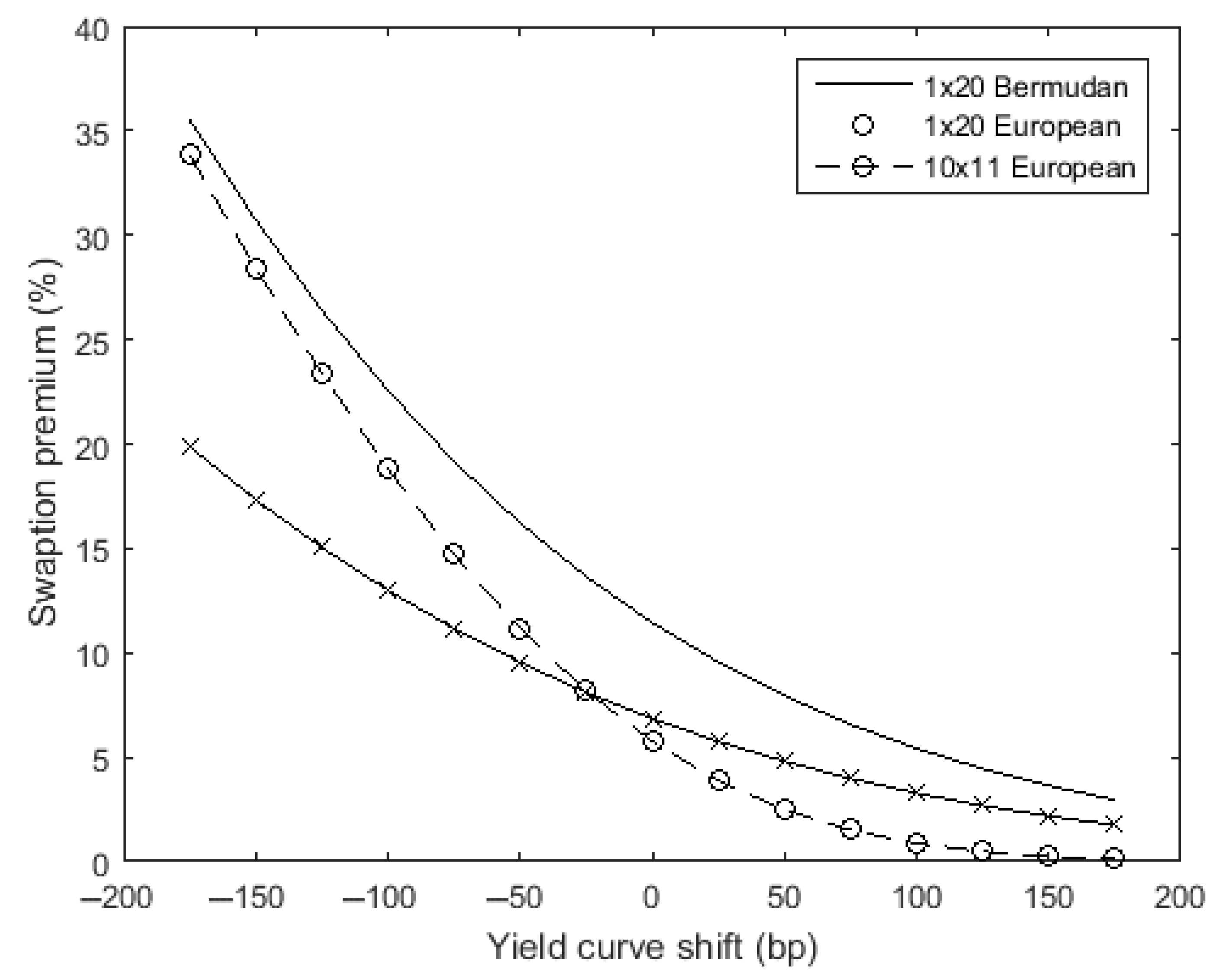
Figure 2 shows the price of the 10Y Bermudan receiver plotted against the prices of its co-terminal European swaptions, all struck at the same rate, $K=1.66\%$. Evidently, the Bermudan price is higher than each of the Europeans in the “basket” and the gap is tightest for the 3Y-into-8Y swaption, which is therefore the MEE. Both the size of the MEE gap and the MEE swaption itself are likely to depend on a combination of market factors, most importantly yield curve level and steepness, as well as forward swap rate volatilities and correlations. For example, while the 3 × 8 swaption is the MEE for the 1 × 10 Bermudan at current prices, under a significant fall in market interest rates, a 1 × 10 swaption would become the MEE, and should rates rise a 6 × 5 European would become the MEE. The MEE basis in these scenarios would fluctuate from 30 to 200 bp (Figure 3).

4.1. Numerical Methods for Pricing Models

Consider now a tenor structure $\mathcal{T}={\left\{T_n\right\}}_{n=\alpha }^{\beta }$ and a “$T_{\beta }$ no-call $T_{\alpha }$” Bermudan receiver swaption introduced above with time t value ${\mathbf{RBS}}_{\alpha ,\beta }(t,K)$. Assuming no prior exercise, at any time point $T_n$ the swaption holder has the right to receive the exercise value $V_e$ of the swaption, i.e., present value of the underlying swap:

$$V_e\left(T_n\right)\equiv {\left(K-S_{n,\beta }\left(T_n\right)\right)}^{+}\sum _{k=n+1}^{\beta }P(T_n,T_k){\delta }_k.$$

(45)

The exercise value has to be compared to the so-called continuation value, $V_c$, of holding the option beyond $T_n$:

$$V_c\left(T_n\right)\equiv \mathbb{E}\left({\mathbf{RBS}}_{\alpha ,\beta }(T_{n+1},K)|S_{n,\beta }\left(T_n\right)\right).$$

(46)

The value of the Bermudan swaption can now be given in terms of (45) and (46) via a dynamic programming recursion:

$$\begin{array}{cc}\hfill {\mathbf{RBS}}_{\alpha ,\beta }(T_{\beta -1},K)& =P(T_{\beta -1},T_{\beta }){\delta }_{\beta }{\left(K-S_{\beta -1,\beta }\left(T_{\beta -1}\right)\right)}^{+}\hfill \\ \hfill {\mathbf{RBS}}_{\alpha ,\beta }(T_j,K)& =max\left(V_e\left(T_j\right),V_c\left(T_j\right)\right),\hfill \end{array}$$

(47)

for $j=\beta -2,\beta -3,\dots ,n$. The evaluation of (47) proceeds backward in time: at $T_{\beta -1}$ the value of the Bermudan is known and determined by the standard swaption payoff. This allows us to update the continuation value at $T_{\beta -2}$ by discounting and comparing it to the exercise value prevailing at the time. The procedure of comparing “backwardly-cumulated” continuation value with the immediate exercise value and deciding upon a swaption exercise is repeated until the initial valuation date is reached, at which point the algorithm yields a price estimate for the Bermudan swaption. The calculation of the continuation value is clearly model-dependent and the choice of modeling framework itself often determines the scope of available numerical techniques. Again without pretense of being exhaustive, we shall consider and briefly discuss three main approaches—binomial/trinomial trees, finite difference schemes based on the derivative PDE and Monte Carlo simulation—traditionally applied in the context of the model categories described above. Our focus will not be on the technical details—for which we refer readers to Glasserman [26], Tavella and Randall [48] as well as Mitchell and Griffiths [49]—but rather on the connection between the modeling framework and numerical implementation techniques.

4.1.1. Tree-Based Methods

Perhaps the most classic approach for pricing derivatives with early exercise features, including Bermudan swaptions, is by building a binomial/trinomial tree for the underlying variable using its discretized SDE (forward induction method). Such methods are only feasible for low-dimensional processes (ideally one- or two-dimensional), which is why they have been extensively used in modeling one-factor short rate models, all of which can be approximated with lattices. Specifically, when approximating a one-factor interest rate diffusion on a trinomial tree, it is assumed that at each time $t_i$ from a discretized domain of time points $0=t_0<t_1<\dots <t_n=T$ (note that the time points in general do not need to be uniformly spaced) there is a finite number of equispaced interest rate states $r_{i,j}$ (i corresponds to the time point and j to the space index), and at each node $(i,j)$ the short rate can move to $r_{i+1,k+1}$, with probability $p_u,$$r_{i+1,k}$ with probability $p_m$, or $r_{i+1,k-1}$, with probability $p_d$, whereby the branching parameters are determined in such a way as to ensure that the conditional mean and variance match as closely as possible their model values. For example, in a simple brute-force implementation of the Hull–White model (17), the probabilities associated with the node $(i,j)$ are:

$$\begin{array}{cc}\hfill p_u& =\frac{{\sigma }^2\Delta t+{({\mu }_{i,j}+(j-k)\Delta r)}^2}{2\Delta r^2}+\frac{{\mu }_{i,j}+(j-k)\Delta r}{2\Delta r}\hfill \\ \hfill p_m& =1-\frac{{\sigma }^2\Delta t+{({\mu }_{i,j}+(j-k)\Delta r)}^2}{\Delta r^2}\hfill \\ \hfill p_d& =1-p_u-p_m\hfill \end{array}$$

where ${\mu }_{i,j}=(\theta (i\Delta t)+\kappa r_{i,j})\Delta t$ is the drift and we have omitted the dependence of transition probabilities on nodes to ease notation. Clearly, building a tree requires as an input the values for short rate volatility $\sigma$ and mean reversion speed $\kappa$, while for numerical stability and convergence considerations $\Delta r=\sigma \sqrt{3\Delta t}$ (in fact, this procedure can be improved upon as explained, e.g., in Hull and White [50]).

The Hull–White model is particularly convenient for pricing Bermudans because knowledge of the short rate is tantamount to the knowledge of all bond prices through the closed reconstitution Formula (20), and thus once an interest rate tree is built along the lines sketched above, we can immediately value all relevant payoffs. Thus, starting from $T_{\beta -1}$, i.e., the last time the swaption can be exercised, and using the readily available bond prices, we calculate for all nodes j in the current column the value ${\mathbf{RBS}}_{\alpha ,\beta }^j(T_{\beta -1},K)$ as:

$$P^j(T_{\beta -1},T_{\beta }){\delta }_{\beta }{\left(K-S_{\beta -1,\beta }^j\left(T_{\beta -1}\right)\right)}^{+}=P^j(T_{\beta -1},T_{\beta }){\delta }_{\beta }{\left(K-\frac{1-P^j(T_{\beta -1},T_{\beta })}{{\delta }_{\beta }{P}^j(T_{\beta -1},T_{\beta })}\right)}^{+}$$

(48)

We then propagate these continuation values backward in time through the interval $T_{\beta -1}=t_{d(\beta -1)}>t_{d(\beta -1)-1}>\dots >t_{d\left(0\right)}=T_{\beta -2}$ using the Formula (46) and the transition probabilities, obtaining “backwardly cumulated” continuation values for each node:

$$V_c^j\left(t_i\right)=p_u{V}_c^{k+1}\left(t_{i+1}\right)+p_m{V}_c^{k+1}\left(t_{i+1}\right)+p_d{V}_c^{k+1}\left(t_{i+1}\right),i=d\left(0\right),\dots ,d(\beta -1)-1$$

(49)

Once the exercise point $T_{\beta -2}$ is reached we check the exercise opportunity by comparing $V_c^j\left(T_{\beta -2}\right)$ with the exercise value:

$$V_e^j\left(T_{\beta -2}\right)={\left(K-S_{\beta -2,\beta }^j\left(T_{\beta -2}\right)\right)}^{+}\left[P^j(T_{\beta -2},T_{\beta -1}){\delta }_{\beta -1}+P^j(T_{\beta -2},T_{\beta }){\delta }_{\beta }\right]$$

(50)

and update the option value accordingly. Proceeding in this way we finally reach the first exercise date $T_{\alpha }$ and subsequently the initial node of the tree with the time 0 swaption price.

While the method sketched in general terms above can be optimized and/or generalized along various dimensions (e.g., varying the discretization step, or including backward propagation of bond prices where no analytical reconstitution formulas are available as in the Black–Karasiński model) it should come as no surprise that the tree can only efficiently handle low-factor short rate rate models. Building a binomial tree for the Hull–White two-factor model is still relatively straightforward; however the added layers of computational complexity seem to defeat the purpose of using a simple (simplistic?) model of the term structure in the first place.

4.1.2. Finite Difference Schemes

The trinomial trees discussed above are in fact a special kind of the so-called explicit finite difference scheme and as such are only conditionally stable. A more efficient method of handling Bermudans in low-factor models, by directly discretizing the partial differential equation for the swaption price, can be deployed as follows. Recall first that if $x\left(t\right)$ is the state variable of the model—driving the discount curve and all its derivables—then by no-arbitrage arguments, the swaption price $V(t,x)$ can be expressed as the risk-neutral expectation of the terminal payoff $V(T,x(T\left)\right)$. Now, since $V(t,x)$ is a martingale, its drift must be zero (in the appropriate measure), and hence applying Ito’s lemma and writing down the dynamics $dV$, we find that $V(t,x)$ must satisfy the following parabolic partial differential equation (PDE):

$$\frac{\partial V(t,x)}{\partial t}+\mathcal{A}V(t,x)=0,$$

(51)

where

$$\mathcal{A}=\underset{\epsilon \to 0}{lim}\frac{{\mathbb{E}}^{\mathbb{Q}}\left(V(t+\epsilon ,x+\epsilon |x\left(t\right)=x\right)-V(t,x)}{\epsilon }$$

(52)

is the infinitesimal operator for the SDE describing the dynamics of the state variable. For example, in the special case of the Hull–White model, the European swaption price solves the following parabolic PDE:

$$\begin{array}{cc}\hfill \frac{\partial V(t,r(t\left)\right)}{\partial t}+\frac{1}{2}\sigma {\left(t\right)}^2\frac{{\partial }^{2}V(t,r\left(t\right))}{\partial r^2}+\left(\theta \left(t\right)-\kappa r\left(t\right)\right)\frac{\partial V(t,r(t\left)\right)}{\partial r}& =r\left(t\right)V(t,r(t\left)\right)\hfill \end{array}$$

Analogously, in the Cheyette model, i.e., Equations (38) and (39), the pricing PDE takes the following form:

$$\begin{array}{cc}\hfill \left(x\right(t)+f(0,t\left)\right)V(t,x(t),y(t\left)\right)=& \frac{\partial V(t,x(t),y(t\left)\right)}{\partial t}\hfill \\ \hfill +& \frac{1}{2}\sigma {\left(t\right)}^2\frac{{\partial }^{2}V(t,x\left(t\right),y\left(t\right))}{\partial x^2}\hfill \\ \hfill +& \left(y\left(t\right)-\kappa x\left(t\right)\right)\frac{\partial V(t,x(t),y(t\left)\right)}{\partial x}\hfill \\ \hfill +& (\sigma {\left(t\right)}^2-2\kappa y\left(t\right))\frac{\partial V(t,x(t),y(t\left)\right)}{\partial y}.\hfill \end{array}$$

Associated with both equations is of course the known terminal swaption payoff condition.

To solve Equation (51) numerically, we discretize it on some finite rectangular domain $[0,T]\times [x_{min},x_{max}]$, where the grid boundaries $x_{min}$ and $x_{max}$ are either determined a priori as some multiples of the variance of $x\left(T\right)$ or within the PDE itself. The partial derivatives are then replaced by corresponding finite difference operators, with schemes differing i.a. in the nature of approximation. The central difference approximation of $\partial V/\partial t$, known as the Crank–Nicolson scheme, is often the method of choice (second-order convergent in $\Delta t$), whereas the backward approximation—given the explicit scheme—should be avoided for stability and convergence considerations. Specifically, for the Crank–Nicolson scheme,

$$\left[\mathbf{I}-\frac{1}{2}{\Delta }_t\mathbf{T}\left(\frac{t_{i+1}+t_i}{2}\right)\right]\widehat{\mathbf{V}}\left(t_i\right)=\left[\mathbf{I}+\frac{1}{2}{\Delta }_t\mathbf{T}\left(\frac{t_{i+1}+t_i}{2}\right)\right]\widehat{\mathbf{V}}\left(t_{i+1}\right),$$

(53)

where I is the identity matrix, $\widehat{\mathbf{V}}\left(t\right)={[\widehat{V}(t,x_{min}),\dots ,\widehat{V}(t,x_{max})]}^{⊺}$ and $\widehat{V}(t,x)$ stands for the approximation to the true solution $V(t,x)$, and $\mathbf{T}$ is a tri-diagonal matrix of coefficients derived from approximating PDE terms. For a known $\widehat{\mathbf{V}}\left(t_{i+1}\right)$, (53) is simply a linear system of equations to be solved by standard methods. Thus, starting from the terminal condition $V(T,x)$—where the swaption payoff is known—we use Equation (53) to iterate backwards in time until we get to $\widehat{\mathbf{V}}\left(0\right)$. Of course, since we are dealing with Bermudan swaptions, at each time step corresponding to exercise time, we additionally need to compare the rollback value with the exercise value—just as has been done on the trinomial tree.

Multi-dimensional PDEs for pricing within the two-factor Hull–White or Cheyette models can still be handled efficiently using the so-called alternating direction implicit method (ADI), introduced by Craig and Sneyd [51]. However, it should be borne in mind that the computational complexity of such problems grows exponentially in the dimension, making it prohibitively inefficient to use finite difference schemes for pricing Bermudans in truly multi-factor models of the term structure.

4.1.3. Monte Carlo

An obvious conclusion would therefore be to switch to Monte Carlo simulation, where the computational cost grows only linearly in dimension. Unfortunately, by design, Monte Carlo simulation works forward in time and therefore dynamic programming of the kind we used above to value Bermudans is not straightforward to implement. A brute-force approach to computing the conditional expectation underlying the continuation value at $T_n$, as per Equation (46), would consist in nesting a new simulation— within the original one—with an initial condition $S_{n,\beta }\left(T_n\right)$, for every $T_n$ and each simulation path, and then calculating the expectation directly. Thus, if the simulation consistently uses M paths, then at time 0 we have M paths, at $t_1$ we generate additional $M^2$ paths, and so on until at the penultimate exercise date $t_N=T_{\beta -1}$ we produce another $M^N$ simulation paths (this time spanning just the final fixing period $[T_{\beta -1},T_{\beta }]$). Clearly, even for a modest choice of M and N the computational burden of such an embedded scheme becomes prohibitive.

This subtle yet crucial point had arguably been one of the key hindrances holding back the financial industry’s embrace of multi-factor market models. Whether many factors per se are desirable for accurate valuation of Bermudans or not—we shall see below that the question is in general not trivial—if they are not amenable to efficient numerical implementation, then they are of little practical significance. A breakthrough came with Longstaff and Schwartz [25], who adapted earlier ideas found in Tilley [52] and Carriere [53], suggesting that the continuation value (46) can be interpreted as a regression of the one-step-ahead payout on the state variables. Indeed, recall that

$$V_c\left(T_n\right)=\mathbb{E}\left({\mathbf{RBS}}_{\alpha ,\beta }(T_{n+1},K)|S_{n,\beta }\left(T_n\right)\right),n=\beta -1,\beta -2,\dots ,1.$$

(54)

Since the conditional expectation of the swaption payoff is an element of the space of square-integrable functions, it has a countable orthonormal basis and can be represented as a linear function of the elements of the basis. Moreover, in a Markovian model, only current values of the state variables are necessary, so we can write:

$$V_c\left(T_n\right)\equiv {\Psi }_n\left(x\left(T_n\right)\right)={\Psi }_n(x_1\left(T_n\right),\dots ,x_d\left(T_n\right)),$$

(55)

for some unknown function ${\Psi }_n$ and d Markov state variables $x_1\left(t\right),\dots ,x_d\left(t\right)$. Longstaff and Schwartz [25] suggest estimating ${\Psi }_n$—and hence the continuation value—by a linear combination of a finite set of J basis functions

$${\Psi }_n\left(x\left(T_n\right)\right)\approx {\Psi }_n^J\left(x\left(T_n\right)\right)=\sum _{j=1}^J{\lambda }_{n,j}{\psi }_j\left(x\left(T_n\right)\right),$$

(56)

where the weights ${\lambda }_{n,j}$ are determined by least-squares regression on the Monte Carlo paths (typically, to improve quality of fit and run-time performance, only in-the-money paths may be considered, which limits the region on which the conditional expectation is to be estimated). Since the values of the basis functions are independently and identically distributed, it can be shown that the fitted value $\widehat{{\Psi }_n^J}\left(x\left(T_n\right)\right)$ converges in mean-square and in probability to ${\Psi }_n^J\left(x\left(T_n\right)\right)$ as the number of paths goes to infinity, which justifies the method.

Once the basis functions and their loadings are determined, valuation follows the dynamic programing method applied above in the context of finite difference schemes and lattices. Thus the algorithm to perform least-squares Monte Carlo (LSMC) to value a Bermudan might look as follows (for concreteness we assume the pricing model is LMM):

1.

Start by specifying and calibrating a desired form of the LMM (number of factors, correlation etc.) as well as the numeraire for the simulation;

2.

Simulate the desired number of paths ${\omega }_1,\dots ,{\omega }_M$ for the underlying LIBOR rates;

3.

Calculate the numeraire, the value of the underlying swap, the values of the basis functions and the exercise values $V_e$ along each path and on all relevant exercise dates;

4.

Set $\widehat{V_c}\left(T_{\beta -1}\right)=0$ and $V_e\left(T_{\beta -1}\right)={\mathbf{RBS}}_{\alpha ,\beta }(T_{\beta -1},K)=P(T_{\beta -1},T_{\beta }){\delta }_{\beta }{\left(K-S_{\beta -1,\beta }\left(T_{\beta -1}\right)\right)}^{+}$;

5.

Going backward in time, i.e., for $n=\beta -2,\dots ,1$, calculate the weights on the basis functions $\widehat{V_c}\left(T_n\right)={\sum }_{j=1}^J\widehat{{\lambda }_{n,j}}{\psi }_j\left(x\left(T_n\right)\right)$ along all paths $\omega$ through standard error minimization:

$$\sum _{\omega }{\left({\mathbf{RBS}}_{\alpha ,\beta }^{\omega }(T_{n+1},K)-\sum _{j=1}^J\widehat{{\lambda }_{n,j}}{\psi }_j\left(x\left(T_n\right)\right)\right)}^2\to min$$

(57)

and use the resulting estimates to update the swaption values $\begin{array}{cc}\hfill {\mathbf{RBS}}_{\alpha ,\beta }(T_n,K)& =max\left(V_e\left(T_j\right),\widehat{V_c}\left(T_n\right)\right)\hfill \end{array}$;

6.

Return ${\mathbf{RBS}}_{\alpha ,\beta }(T_0,K)$.

Several remarks are in order at this point. First, as should be clear from the discussion above, the robustness of our valuation scheme is critically affected by the choice of the explanatory variables in the regression, i.e., the form and number of the basis functions. In their formulation, Longstaff and Schwartz [25] recommend using a polynomial basis, i.e., monomials of the state variables. While sound in principle, this approach might be impractical in the context of LMM due to the possibly high dimension of the vector of state variables (core LIBOR rates). Note also that with too many regressors, the quality of the parameter estimates is likely to deteriorate, given a fixed number of Monte Carlo paths. For example, Glasserman and Yu [54] show that the number of regression variables for which accurate estimation is possible from M paths is $O(logM)$. Thus with, say, 50,000 paths we should not use more than four variables. A popular choice is to choose i.a. the front LIBOR rate (fixing on the exercise date), and several swap rates capturing the overall level and shape of the yield curve.

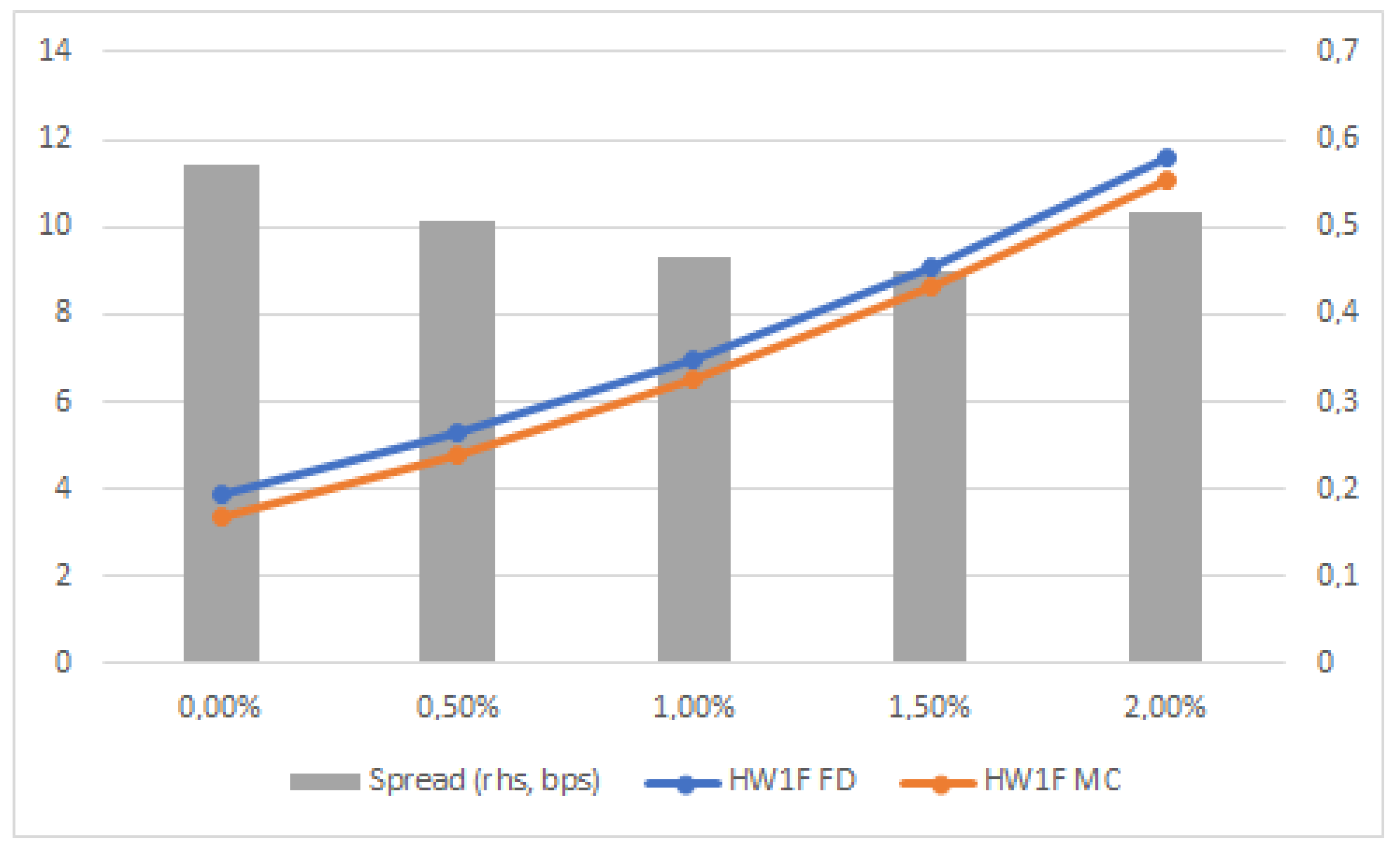
Second, unlike in lattices or finite difference schemes, in LSMC, exercise decisions will be sub-optimal by design as they rest on estimates of continuations values. At the same time, to the extent that the same set of paths is used to determine both the parameters $\widehat{{\lambda }_{n,j}}$ and continuation values, the price estimate might be biased upwards. To reduce bias and make sure that the regression generates a lower bound on the option price, we could use two independent Monte Carlo simulations: the first pilot run to fit the coefficients and then a second run to estimate continuation values for a newly seeded set of paths based on the previously determined decision rule. To gauge the quantitative effect of sub-optimal exercise decisions we conducted a simple experiment in which we priced the same 20-non-call-10 Bermudan swaption with a one-factor Hull–White model using a standard Crank–Nicolson finite-difference grid and LSMC. The model was calibrated to ATM European swaptions with final 20Y maturity, and the mean reversion rate was in each case set at 0.03. The results are shown in Figure 4 and clearly demonstrate the downward bias of the Monte Carlo with spreads relative to the exact finite-difference scheme in the order of 40–50 bps.

4.2. Factor Dependence of Bermudan Swaptions

Having presented the main categories of models and implementation techniques that can be used to price Bermudan swaptions we now turn to the issue of their factor dependence. In particular, using a set of numerical experiments we revisit the debate between Longstaff, Santa-Clara, and Schwartz [9] and Andersen and Andreasen [23], and the threats posed by the modeling equivalents of Scylla and Charybdis mentioned in the introduction.

Consider once again a “$T_{\beta }$ no-call $T_{\alpha }$” Bermudan receiver swaption, which, as we know, can be exercised into one of the so-called core swap rates:

$$S_{\alpha ,\beta }\left(T_{\alpha }\right),S_{\alpha +1,\beta }\left(T_{\alpha +1}\right),\dots ,S_{\beta -1,\beta }\left(T_{\beta }\right)$$

(58)

at either one of the designated exercise times $T_{\alpha },T_{\alpha +1},\dots ,T_{\beta }$, at the same strike rate K. In an important paper Longstaff, Santa-Clara, and Schwartz [9] made a point that this “chooser-option” character of a Bermudan makes is critically sensitive to the correlation among the core rates. Drastically simplifying their argument, we can imagine that when the individual $S_{i,\beta },S_{j,\beta }$ are perfectly correlated, so too should be the respective exercise values. Hence, there is likely to be little value added provided by the option to postpone the exercise. By contrast, the argument goes, when correlation between $S_{i,\beta },S_{j,\beta }$ is low or even negative, a Bermudan’s right to choose the exercise date will have more value. Indeed, if the exercise value of the first swaption happens to be positive, it is worth exercising sooner, as payoffs further down the line are likely to turn negative. A straightforward conclusion follows that since single-factor models by design imply perfect correlation between core swap rates, they should artificially under-price Bermudan swaptions, making traders “throw away billions of dollars.” From a theoretical point of view, the result—coupled with advances in numerical techniques under the guise of LSMC— provided a powerful argument in favor of switching from short-rate to multi-factor market models.

And yet, Andersen and Andreasen [23] pointed out a subtle flaw in the above reasoning: to the extent that our Bermudan is viewed as a chooser option, one has to bear in mind that the choice we refer to is made at different points in time: $T_{\alpha },T_{\alpha +1},\dots ,T_{\beta }$. Consequently, what matters for pricing is not the instantaneous correlation

$$\mathbb{E}\left[d{S}_{i,\beta }\left(t\right)d{S}_{j,\beta }\left(t\right)\right]={\rho }_{i,j}\left(t\right)dt$$

(59)

between the Brownian motions driving the dynamics of the core swap rates, but rather the forward or serial correlation between the rates setting at different dates $T_i$ and $T_j$, which can be very roughly approximated as:

$$\frac{{\int }_0^{T_i}{\sigma }_i\left(t\right){\sigma }_j\left(t\right){\rho }_{i,j}dt}{\sqrt{{\int }_0^{T_i}{\sigma }_i^2\left(t\right)dt}\sqrt{{\int }_0^{T_j}{\sigma }_j^2\left(t\right)dt}},$$

(60)

and depend not just on ${\rho }_{i,j}$ but also on the volatilities of $T_i$- and $T_j$-maturity rates. This shows that while single-factor models do indeed imply perfect instantaneous correlation, they can de-correlate core rates setting at different times (through the time-dependent volatilities), with non-trivial consequences for Bermudan swaptions prices.

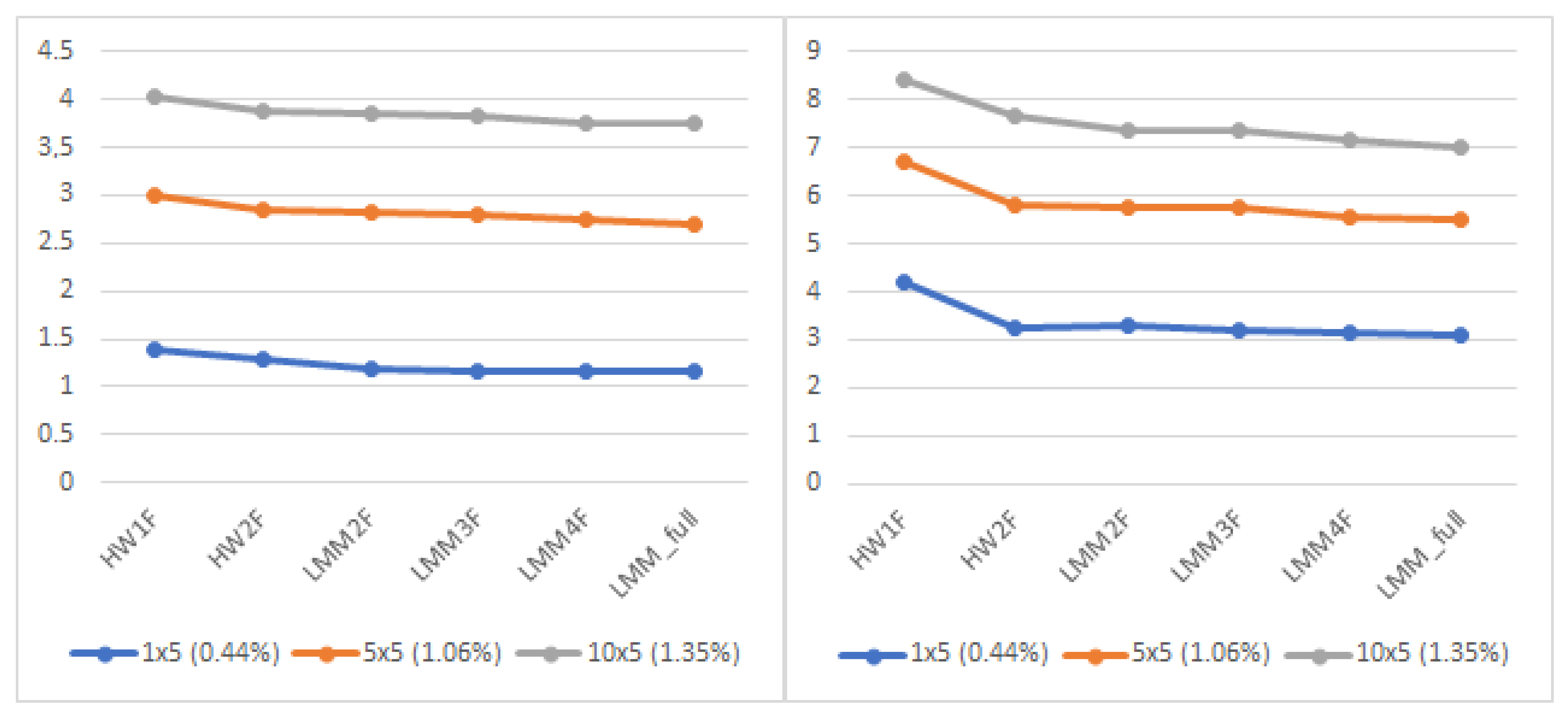
To appreciate this last point, we conducted our own set of numerical experiments using the modeling tools described above. Specifically, we priced Bermudan swaptions on a 5Y and 10Y swap with quarterly payment frequency and time to first exercise set at 1, 5 and 10 years. The strikes in each case were set to ATM levels based on the USD interest rate curve as of 11 September 2020. We used the Hull–White one-factor model (HW1F) implemented on a finite-difference grid as a benchmark and considered its two-factor extension (HW2F), and four versions of the LIBOR market model assuming 2-, 3-, 4- and full-factor parameterization. In line with standard practice, we used a piece-wise constant volatility function and Rebonato’s two-parameter correlation structure of the form ${\rho }_{n,m}={\rho }_{\infty }+(1-{\rho }_{\infty })exp(-{\rho }_{dec}|n-m|)$, for the full-factor model. We used 25,000 pre-simulation paths to fit the coefficients and then another 25,000 with antithetic variates (a total of 50,000 paths) to estimate continuation values based on the previously determined decision rule.

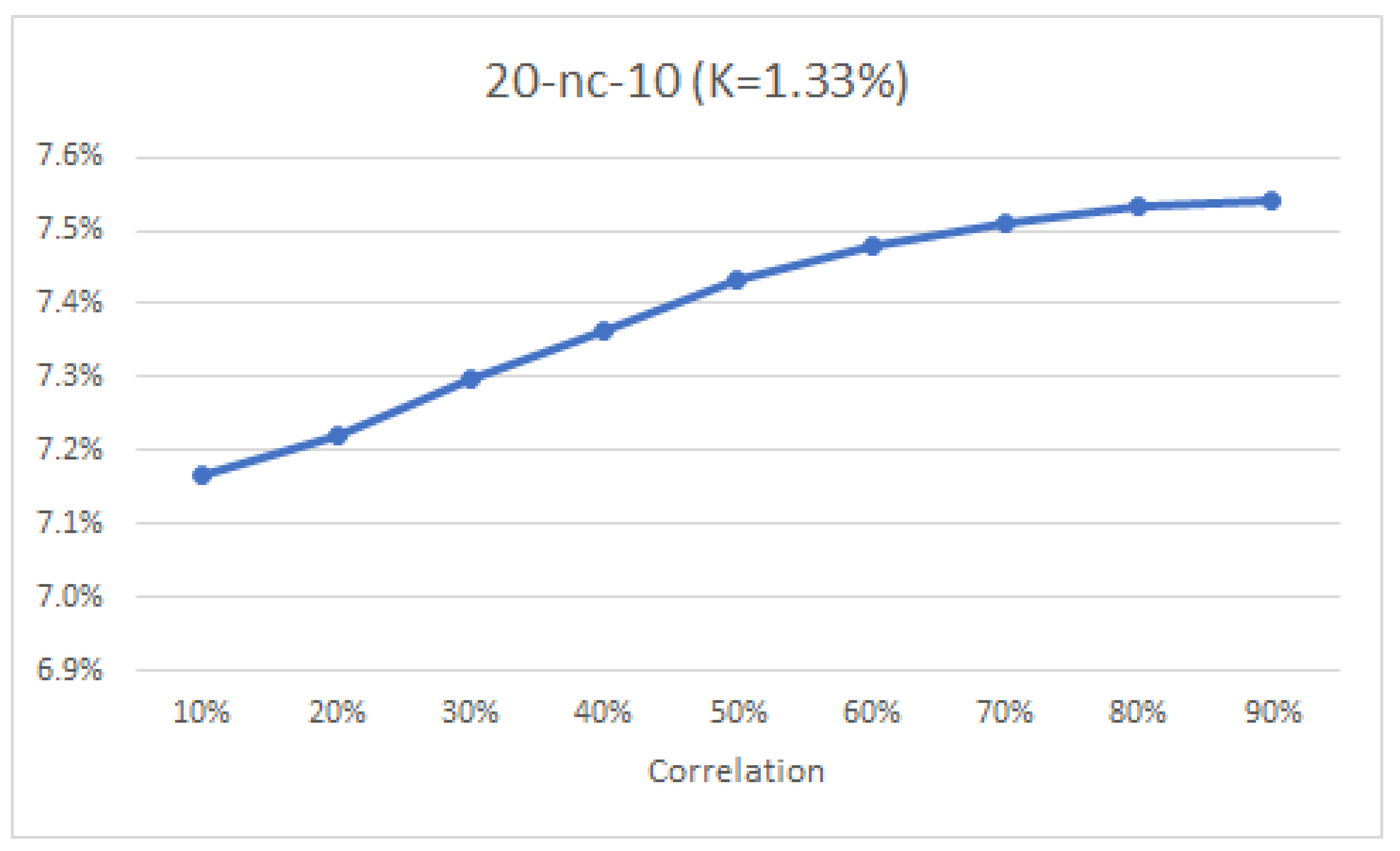
The results of our numerical experiments, shown in Figure 5, are generally in line with those reported in a much more comprehensive study by Andersen and Andreasen [23] and seem to confirm the de-correlation possibilities of low-factor models. Indeed, prices produced by the HW1F model are consistently higher than those derived from the two-, three- and very high-factor market models. For longer-maturity products this pattern can be quite pronounced with the relative error for the 20-nc-10 swaption reaching almost 15%. Whereas a part of this pattern may be due to different numerical procedures employed (grid solution for HW1F and LSMC for other models), our earlier tests, reported in Figure 4, show that this cannot be the entire explanation. Indeed, to assess the dependence of swaption prices on rate correlation, we used our calibrated full-factor LMM to reprice the same 10 × 10 Bermudan receiver (struck at 1.33%) varying base correlation ${\rho }_{\infty }$ from 0.1% to 0.9% (Figure 6). Again, the results show that increasing correlation increases, not decreases, Bermudan swaption prices.

To provide some intuition for these results, we recall that a forward swap rate is a complex average of underlying forward rates, so we can write:

$$S_{\alpha ,\beta }\left(t\right)=\sum _{i=\alpha +1}^{\beta }{w}_i\left(t\right)F_i\left(t\right),$$

(61)

where the weights are given by:

$$w_i\left(t\right)=\frac{{\prod }_{j=\alpha +1}^i\frac{1}{1+{\delta }_j{F}_j\left(t\right)}}{{\sum }_{k=\alpha +1}^{\beta }{\delta }_k{\prod }_{j=\alpha +1}^k\frac{1}{1+{\delta }_j{F}_j\left(t\right)}}.$$

(62)

If we now freeze the weights at their time-zero values—as originally proposed by Jackel and Rebonato [55], Rebonato [56] and justified by the fact that the variability of $w_i$s is significantly smaller than the variability of the LIBOR rates—we can differentiate (61) to obtain:

$$d{S}_{\alpha ,\beta }\left(t\right)\approx \sum _{i=\alpha +1}^{\beta }{w}_i\left(0\right)d{F}_i\left(t\right)=(\dots )dt+\sum _{i=\alpha +1}^{\beta }{w}_i\left(0\right){\sigma }_i\left(t\right)F_i\left(t\right)d{W}_i\left(t\right).$$

(63)

Calculating the quadratic variation and approximating it further by freezing all rates at their time-zero values, we obtain the following approximate expression for integrated percentage variance, or (squared) swap rate volatility:

$${\int }_0^{T_{\alpha }}\frac{d{S}_{\alpha ,\beta }\left(t\right)d{S}_{\alpha ,\beta }\left(t\right)}{S_{\alpha ,\beta }{\left(t\right)}^2}\approx \sum _{i,j=\alpha +1}^{\beta }\frac{w_i\left(0\right)w_j\left(0\right)F_i\left(0\right)F_j\left(0\right){\rho }_{i,j}}{T_{\alpha }{S}_{\alpha ,\beta }{\left(0\right)}^2}{\int }_0^{T_{\alpha }}{\sigma }_i\left(t\right){\sigma }_j\left(t\right)dt$$

(64)

which must be plugged into the Black Formula (12) to recover the market price of a European swaption on the swap fixing in $T_{\alpha }$ and maturing in $T_{\beta }$. Now, if the volatilities of the forward rates spanning the swap are held fixed (e.g., through thorough calibration), then decreasing ${\rho }_{i,j}$ by moving to a lower-factor model or by adjusting the base correlation parameter ${\rho }_{\infty }$ will necessarily also reduce the swap rate volatility—and hence ultimately the price of the Bermudan.

Although other subtle effects can also play a role, justifying more extensive tests than allowed by the scope of this essay (see, e.g., [57,58] and as usual [7] for a general reference), we can nevertheless safely conclude at this point that factor dependency does seem to be an issue in pricing Bermudan swaptions. This empirical conclusion validates our perspective on the evolution of Bermudan swaption pricing as driven by a difficult choice between a more cumbersome and difficult to sensibly calibrate low-factor model that can be more efficiently implemented (Charybdis) and a multi-factor model that allows much more calibration freedom, but raises problems on the numerical implementation front and produces sub-optimal exercise decisions.

5. Markovian Projection and Dimension Reduction

We now consider a novel approach to deal with the “curse of dimensionality”, which rests on the idea of Markovian projection and the seminal contribution of Gyöngy [28], who showed that for every stochastic process with an Ito differential:

$$d\xi \left(t\right)=\delta \left(t\right)dW\left(t\right)+\beta \left(t\right)dt,\xi \left(0\right)=0$$

(65)

there exists a stochastic differential equation:

$$d\chi \left(t\right)=\gamma (t,\chi (t\left)\right)dW\left(t\right)+b(t,\chi (t\left)\right)dt$$

(66)

having the same one-dimensional probability distribution as $\xi \left(t\right)$ for every t, with $\gamma {(t,\chi )}^2=\mathbb{E}\left(\delta {\left(t\right)}^2\right|\xi \left(t\right)=\chi )$ and $b(t,\chi )=\mathbb{E}\left(\beta \right(t\left)\right|\xi \left(t\right)=\chi )$. Below we extend and generalize this result to non-probabilistic measures. This will be more relevant to option pricing, which requires taking expectations of discounted terminal payoffs. Concretely, we will show below that for every pair of stochastic processes:

$$\begin{array}{cc}\hfill d\xi \left(t\right)& =\delta \left(t\right)dW\left(t\right)+\beta \left(t\right)dt,\xi \left(0\right)=0\hfill \\ \hfill dZ\left(t\right)& =z\left(t\right)dW\left(t\right)+\zeta \left(t\right)dt\hfill \end{array}$$

there exist Markovian counterparts $(\chi ,U)$ satisfying the following Ito equations:

$$\begin{array}{cc}\hfill d\chi \left(t\right)& =\delta (t,\chi (t\left)\right)dW\left(t\right)+\beta (t,\chi (t\left)\right)dt\hfill \\ \hfill dU\left(t\right)& =U\left(t\right)\zeta (t,\chi (t\left)\right)dt\hfill \end{array}$$

such that the values $\mathbb{E}\left[Z\left(t\right){𝟙}_{\left\{\xi \right(t)>K\}}\right]$ and $\mathbb{E}\left[U\left(t\right){𝟙}_{\left\{\chi \right(t)>K\}}\right]$ coincide for every t and K. If the function $\zeta$ is negative, then $\mathbb{E}\left[U\left(t\right){𝟙}_{\left\{\chi \right(t)>K\}}\right]=\mathrm{Prob}(\chi \left(t\right)>K)$, where $\chi$ is a Markov process with Ito differential $d\chi \left(t\right)=\delta (t,\chi (t\left)\right)dW\left(t\right)+\beta (t,\chi (t\left)\right)dt$ and killing rate $-\zeta (t,\chi )$. Furthermore, the infinitesimal generator $\mathcal{A}$ of such a process is given by:

$$\mathcal{A}h\left(\chi \right)=\frac{1}{2}\delta (t,\chi )h^{″}\left(\chi \right)+\beta (t,\chi )h^{\prime }\left(\chi \right)+\zeta (t,\chi )h\left(\chi \right).$$

(67)

The practical significance of this result is easy to see. Since $\xi (·)$ and $\chi (·)$ have the same marginal probability distributions, it follows that prices of all European options on $\xi (·)$ and $\chi (·)$ will be equal, for any expiration time t. For our present purposes this means that even if the swap rate evolves according to some very high-factor model with a stochastic volatility, we can replace it with a much simpler model by “localizing” its parameters, effectively reducing dimensionality. And while in theory this only guarantees that we match European options prices, we shall see below that a Markovian process for the swap rate—with a number of freezing approximations—provides a simple and robust tool for pricing Bermudan swaptions.

5.1. Markovian Projection for the Swap Rate

Consider once again the forward swap rate $S_{\alpha ,\beta }$ defined in continuous-time convention by Equation (10), and the corresponding $T_{\alpha }$-expiry European swaption with time-zero price:

$${\mathbb{E}}^{\mathbb{Q}}\left[\frac{N_{\alpha ,\beta }\left(T_{\alpha }\right)}{B\left(T_{\alpha }\right)}{\left(S_{\alpha ,\beta }\left(T_{\alpha }\right)-K\right)}^{+}\right].$$

(68)

If both the expectation and the underlying swap rate are viewed, counter-intuitively, as functions of $T_{\alpha }=t$, then (for fixed $T_{\beta }=T$) there arise two spot processes:

$$C(t,K)\equiv {\mathbb{E}}^{\mathbb{Q}}\left[\frac{N\left(t\right)}{B\left(t\right)}{\left(S\left(t\right)-K\right)}^{+}\right],S\left(t\right)\equiv S_{t,T}\left(t\right)$$

(69)

For notational convenience denote $D\left(t\right)=\frac{N\left(t\right)}{B\left(t\right)}$ and $F\left(t\right)=D\left(t\right)S\left(t\right)$ so that:

$$\begin{array}{cc}C(t,K)& ={\mathbb{E}}^{\mathbb{Q}}\left[D\left(t\right){\left(S\left(t\right)-K\right)}^{+}\right].\end{array}$$

(70)

Now, suppose that the dynamics of $S\left(t\right)$ is described by some potentially complicated high-factor model with the following SDE:

$$dS\left(t\right)=\phi \left(t\right)dW\left(t\right)-(\dots )dt$$

(71)

Note that the notation suggesting that $dW\left(t\right)$ is one-dimensional involves no loss of generality since for any multi-dimensional process we can always find a diffusion and one-dimensional Brownian motion such that laws of both processes exactly match.

It is straightforward to calculate that:

$$dD\left(t\right)=(\dots )d{W}_1\left(t\right)-B\left(t\right)dt$$

(72)

and

$$dF\left(t\right)=(\dots )d{W}_2-B\left(t\right)r\left(t\right)dt.$$

(73)

for some Wiener processes $W_1$ and $W_2$.

We now present the main result in the form of the following theorem.

Theorem 1.

Let $S\left(t\right),D\left(t\right)$ and $F\left(t\right)$ be stochastic processes with general Ito differentials (71)–(73). Then there exists a pair of processes $\left(Z\right(t),Q(t\left)\right)$ with dynamics

$$dZ\left(t\right)=\phi (t,Z\left(t\right))dW\left(t\right)+\left(g(t,Z(t\left)\right)-Z\left(t\right)h(t,Z(t\left)\right)\right)dt$$

(74)

$$dQ\left(t\right)=Q\left(t\right)h(t,Z(t\left)\right)$$

(75)

such that the discounted one-dimensional distributions of $S\left(t\right)$ and $Z\left(t\right)$ are equivalent, i.e., ${\mathbb{E}}^{\mathbb{Q}}\left[D\left(t\right){𝟙}_{\left\{S\right(t)>K\}}\right]={\mathbb{E}}^{\mathbb{Q}}\left[Q\left(t\right){𝟙}_{\left\{Z\right(t)>K\}}\right]$ for every $t,K$. The coefficients φ,$g,h$ are non-random and have the following simple interpretation: ${\phi }^2(t,x)={\mathbb{E}}^t\left[{\phi }^2\left(t\right)|S\left(t\right)=x\right]$, $g(t,x)=-{\mathbb{E}}^t\left[\left.\frac{r\left(t\right)}{N\left(t\right)}\right|S\left(t\right)=x\right]$, and $h(t,x)=-{\mathbb{E}}^t\left[\left.\frac{1}{N\left(t\right)}\right|S\left(t\right)=x\right]$, where ${\mathbb{E}}^t[·]$ is the expectation under t-forward measure defined by:

$${\mathbb{E}}^t\left(\xi \right)\equiv \frac{{\mathbb{E}}^{\mathbb{Q}}\left[D\left(t\right)\xi \right]}{{\mathbb{E}}^{\mathbb{Q}}\left[D\left(t\right)\right]}$$

(76)

for any ξ.

Remark 1.

The Theorem above can be seen as a generalization of the result due to Gyöngy [28], who first observed that it is possible to construct a process that mimics the one-dimensional distributions of a given Ito process, but is simpler in the sense that its drift and diffusion terms are non-random, localized versions of the drift and diffusion of the original process (which in general may themselves be stochastic processes). We offer a reinterpretation and extension of the result to cover non-probabilistic and discounted distributions relevant in option pricing. Therefore, the proof we present below is finance-motivated and starts by considering the swaption payoff spot process as per Equation (70).

Proof. 

By Tanaka’s formula,

$$d{(S\left(t\right)-K)}^{+}={𝟙}_{\left\{S\right(t)>K\}}dS\left(t\right)+\frac{1}{2}\delta (S\left(t\right)-K)d{〈S\left(t\right)〉}_t.$$

(77)

Hence, recalling Equation (70), we can calculate the dynamics of $C(t,K)$ as: use

$$\begin{array}{cc}\hfill d\left(D\left(t\right){(S\left(t\right)-K)}^{+}\right)=& \frac{1}{2}{\phi }^2\left(t\right)\delta (S\left(t\right)-K)D\left(t\right)dt+{𝟙}_{\left\{S\right(t)>K\}}\left[D\left(t\right)dS\left(t\right)+d{〈S,D〉}_t\right]+{(S\left(t\right)-K)}^{+}dD\left(t\right)\hfill \\ \hfill =& \frac{1}{2}{\phi }^2\left(t\right)\delta (S\left(t\right)-K)D\left(t\right)dt+{𝟙}_{\left\{S\right(t)>K\}}\left[D\left(t\right)dS\left(t\right)+d{〈S,D〉}_t+(S\left(t\right)-K)dD\left(t\right)\right]\hfill \\ \hfill =& \frac{1}{2}{\phi }^2\left(t\right)\delta (S\left(t\right)-K)D\left(t\right)dt+{𝟙}_{\left\{S\right(t)>K\}}\left[dF\left(t\right)-KdD\left(t\right)\right].\hfill \end{array}$$

Taking the expected value of both sides under the risk neutral measure $\mathbb{Q}$ yields:

$$\frac{\partial C(t,K)}{\partial t}={\mathbb{E}}^{\mathbb{Q}}\left[\frac{1}{2}D\left(t\right)\delta (S\left(t\right)-K){\phi }^2\left(t\right)\right]+{\mathbb{E}}^{\mathbb{Q}}\left[{𝟙}_{\left\{S\right(t)>K\}}\left(-B\left(t\right)r\left(t\right)-KB\left(t\right)\right)\right].$$

(78)

Since $C(t,x)={\mathbb{E}}^{\mathbb{Q}}\left[D\left(t\right){(S\left(t\right)-x)}^{+}\right]={\mathbb{E}}^{\mathbb{Q}}\left[D\left(t\right)\right]{\mathbb{E}}^t\left[{(S\left(t\right)-x)}^{+}\right]$, the probability distribution of S in the t-forward measure ${\mathbb{Q}}^t$ is:

$$\frac{1}{{\mathbb{E}}^{\mathbb{Q}}\left[D\left(t\right)\right]}{\partial }_{xx}^{2}C(t,x).$$

(79)

Hence,

$$\begin{array}{cc}\hfill {\mathbb{E}}^{\mathbb{Q}}\left[\frac{1}{2}D\left(t\right)\delta (S\left(t\right)-K){\phi }^2\left(t\right)\right]& =\frac{1}{2}{\mathbb{E}}^{\mathbb{Q}}\left[D\left(t\right)\right]{\mathbb{E}}^t\left[\delta (S\left(t\right)-K){\phi }^2\left(t\right)\right]\hfill \\ \hfill & =\frac{1}{2}\mathbb{E}\left[D\left(t\right)\right]{\mathbb{E}}^t\left[\delta \left(S\right(t)-K)\right]{\mathbb{E}}^t\left[{\phi }^2\left(t\right)|S\left(t\right)=K\right]\hfill \\ \hfill & =\frac{1}{2}\frac{{\partial }^{2}C(t,x)}{\partial x^2}{\mathbb{E}}^t\left[{\phi }^2\left(t\right)|S\left(t\right)=x\right].\hfill \end{array}$$

(80)

Observe now that:

$$\begin{array}{cc}\hfill {\mathbb{E}}^{\mathbb{Q}}\left[{𝟙}_{\left\{S\right(t)>K\}}\left(-B\left(t\right)r\left(t\right)-KB\left(t\right)\right)\right]& ={\mathbb{E}}^{\mathbb{Q}}\left[\frac{D\left(t\right)}{D\left(t\right)}{𝟙}_{\left\{S\right(t)>K\}}\left(-B\left(t\right)r\left(t\right)-KB\left(t\right)\right)\right]\hfill \\ \hfill & ={\mathbb{E}}^{\mathbb{Q}}\left[D\left(t\right)\right]{\mathbb{E}}^t\left[{𝟙}_{\left\{S\right(t)>K\}}\frac{-B\left(t\right)r\left(t\right)-KB\left(t\right)}{D\left(t\right)}\right].\hfill \end{array}$$

Pick a sequence ${\left(x_n\right)}_{n=0}^{\infty }$ of evenly spaced numbers such that $x_0=K$, $x_{i+1}-x_i=\Delta$ and ${lim}_{n\to \infty }{x}_n=\infty$. Then we may write:

$$\begin{array}{cc}\hfill {\mathbb{E}}^t\left[{𝟙}_{\left\{S\right(t)>K\}}\frac{B\left(t\right)r\left(t\right)}{D\left(t\right)}\right]& =\sum _{i=0}^{\infty }{\mathbb{E}}^t\left[{𝟙}_{\{x_i<S\left(t\right)<x_{i+1}\}}\frac{B\left(t\right)r\left(t\right)}{D\left(t\right)}\right]\hfill \\ \hfill & =\sum _{i=0}^{\infty }{\mathbb{E}}^t\left[\left.\frac{B\left(t\right)r\left(t\right)}{D\left(t\right)}\right|x_i<S\left(t\right)<x_{i+1}\right]{\mathbb{P}}^t\left(x_i<S\left(t\right)<x_{i+1}\right).\hfill \end{array}$$

Letting $\Delta \to 0$, and using Equation (79), we obtain:

$${\mathbb{E}}^t\left[{𝟙}_{\left\{S\right(t)>K\}}\frac{B\left(t\right)r\left(t\right)}{D\left(t\right)}\right]=\frac{1}{{\mathbb{E}}^{\mathbb{Q}}\left[D\left(t\right)\right]}{\int }_K^{\infty }\frac{{\partial }^{2}C(t,x)}{\partial x^2}{\mathbb{E}}^t\left[\left.\frac{B\left(t\right)r\left(t\right)}{D\left(t\right)}\right|S\left(t\right)=x\right]dx.$$

(81)

Analogously,

$${\mathbb{E}}^t\left[{𝟙}_{\left\{S\right(t)>K\}}\frac{KB\left(t\right)}{D\left(t\right)}\right]=\frac{1}{{\mathbb{E}}^{\mathbb{Q}}\left[D\left(t\right)\right]}{\int }_K^{\infty }{\partial }_{xx}^2\frac{{\partial }^{2}C(t,x)}{\partial x^2}K{\mathbb{E}}^t\left[\left.\frac{B\left(t\right)}{D\left(t\right)}\right|S\left(t\right)=x\right]dx.$$

(82)

Using (80)–(82) we can finally re-express Equation (78) as:

$$\frac{\partial C(t,x)}{\partial t}=\frac{1}{2}\frac{{\partial }^{2}C(t,x)}{\partial x^2}{\phi }^2(t,x)+{\int }_K^{\infty }\frac{{\partial }^{2}C(t,x)}{\partial x^2}\left[g(t,x)-Kh(t,x)\right]dx.$$

(83)

Differentiating (83) twice with respect to the strike rate gives us the Fokker–Planck equation:

$$\begin{array}{cc}\hfill \frac{{\partial }^{3}C(t,x)}{\partial t\partial x^2}& =\frac{1}{2}\frac{{\partial }^2}{\partial K^2}\left\{\frac{{\partial }^{2}C(t,x)}{\partial x^2}{\phi }^2(t,x)\right\}\hfill \\ \hfill & +\frac{\partial }{\partial K}\left\{\frac{{\partial }^{2}C(t,x)}{\partial x^2}\left[g(t,x)-Kh(t,x)\right]\right\}-\frac{{\partial }^{2}C(t,K)}{\partial K^2}h(t,K)\hfill \end{array}$$

(84)

which describes the time evolution of the probability density implied by swaptions prices $\{C{(t,K\}}_{t,K}$. Note that the unique Markovian solution to Equation (84) is a pair of processes $\left(Z\right(t),Q(t\left)\right)$ with the following dynamics:

$$dZ\left(t\right)=\phi (t,Z\left(t\right))dW\left(t\right)+\left(g(t,Z(t\left)\right)-Z\left(t\right)h(t,Z(t\left)\right)\right)dt$$

(85)

$$dQ\left(t\right)=Q\left(t\right)h(t,Z(t\left)\right)$$

(86)

It follows that ${\partial }_{xx}^{2}C(t,x)$ is the “Q-discounted” density of $Z\left(t\right)$ and clearly also the “D-discounted” density of $S\left(t\right)$, as desired. □

Remark 2.

The discounting referred to in the proof is crucial: while the distributions of $S\left(t\right)$ and $Z\left(t\right)$ are not equivalent, it nonetheless holds that:

$${\mathbb{E}}^{\mathbb{Q}}\left[D\left(t\right){𝟙}_{\left\{S\right(t)>K\}}\right]={\mathbb{E}}^{\mathbb{Q}}\left[Q\left(t\right){𝟙}_{\left\{Z\right(t)>K\}}\right]$$

(87)

and non-probabilistic measures ${\mathbb{P}}^D\left[S\left(t\right)>K\right]$ and ${\mathbb{P}}^Q\left[Z\left(t\right)>K\right]$ are equivalent.

As a corollary, observe that the equivalence of non-probabilistic measures implies the equivalence of swaption prices:

$$C(t,K)={\mathbb{E}}^{\mathbb{Q}}\left[D\left(t\right){\left(S\left(t\right)-K\right)}^{+}\right]={\mathbb{E}}^{\mathbb{Q}}\left[Q\left(t\right){\left(Z\left(t\right)-K\right)}^{+}\right],$$

(88)

which in turn implies that functions $h(t,K)$ and $g(t,K)$ are given in closed form. Indeed,

$${\mathbb{E}}^{\mathbb{Q}}\left[exp\left(-{\int }_0^{t}r\left(s\right)ds\right){𝟙}_{\left\{S\right(t)>K\}}\right]=-{\int }_K^{\infty }\frac{{\partial }^{2}C(t,x)}{\partial x^2}h(t,x)dx$$

(89)

and

$$h(t,K)={\left(\frac{{\partial }^{2}C(t,x)}{\partial x^2}\right)}^{-1}\frac{\partial {\mathbb{E}}^{\mathbb{Q}}\left[exp\left(-{\int }_0^{t}r\left(s\right)ds\right){𝟙}_{\left\{S\right(t)>K\}}\right]}{\partial K}.$$

(90)

Analogously,

$${\mathbb{E}}^{\mathbb{Q}}\left[exp\left(-{\int }_0^{t}r\left(s\right)ds\right){𝟙}_{\left\{S\right(t)>K\}}r\left(t\right)\right]=-{\int }_K^{\infty }\frac{{\partial }^{2}C(t,x)}{\partial x^2}g(t,x)dx,$$

(91)

and

$$g(t,K)={\left(\frac{{\partial }^{2}C(t,x)}{\partial x^2}\right)}^{-1}\frac{\partial {\mathbb{E}}^{\mathbb{Q}}\left[exp\left(-{\int }_0^{t}r\left(s\right)ds\right){𝟙}_{\left\{S\right(t)>K\}}r\left(t\right)\right]}{\partial K}.$$

(92)

Note that owing to the matching of one-dimensional (discounted) distributions, the equality of European options prices on $S(·)$ and $Z(·)$ is exact. However, Markovian projection does not preserve higher-order distributions, and therefore, in general, (88) does not extend automatically to Bermudan swaptions. That said, we can hope that:

$$\begin{array}{cc}\hfill {\mathbf{RBS}}_{\alpha ,\beta }(t,K)& =\underset{\tau \in \mathcal{T}}{sup}{\mathbb{E}}^{\mathbb{Q}}\left[\frac{N_{\tau ,\beta }\left(\tau \right)}{B\left(\tau \right)}{\left(K-S_{\tau ,\beta }\left(\tau \right)\right)}^{+}\right]\hfill \end{array}$$

(93)

$$\begin{array}{cc}\hfill & =\underset{\tau \in \mathcal{T}}{sup}{\mathbb{E}}^{\mathbb{Q}}\left[D\left(\tau \right){\left(K-S\left(\tau \right)\right)}^{+}\right]\approx \underset{\tau \in \mathcal{T}}{sup}{\mathbb{E}}^{\mathbb{Q}}\left[Q\left(\tau \right){\left(K-Z\left(\tau \right)\right)}^{+}\right]\hfill \end{array}$$

(94)

Whether and to what extent Equation (93) holds is ultimately an empirical matter, but our numerical experiments reported below suggest that the approximation is in fact good enough to justify its practical use.

5.2. Parameter Approximations and Numerical Experiments

Our strategy now is to calculate the right-hand side of (93) and compare the obtained price—across a range of strikes—to ${\mathbf{RBS}}_{\alpha ,\beta }(t,K)$ determined using a proper multi-factor model. Perhaps the most straightforward way involves stripping the functions $g(·,·)$ and $h(·,·)$ off the interest rate curve and market swaptions prices using Formulas (90)–(92). But we outline here an even simpler strategy suggested in Gatarek and Jabłecki [59]. Concretely, we assume that

$$P(t,T)\approx \frac{P(0,T)}{P(0,t)},$$

(95)

which implies that

$$P(0,t){\int }_t^{T}P(t,s)ds\approx {\int }_t^{T}P(0,s)ds,$$

(96)

so that

$$\frac{r\left(t\right)}{N\left(t\right)}=\frac{r\left(t\right)S\left(t\right)}{1-P(t,T)}\approx \frac{f(0,t)P(0,t)}{P(0,t)-P(0,T)}S\left(t\right)$$

(97)

and

$$\frac{1}{N\left(t\right)}\approx \frac{P(0,t)}{{\int }_t^{T}P(0,s)ds}$$

(98)

Set $p\left(t\right)\equiv \frac{f(0,t)P(0,t)}{P(0,t)-P(0,T)}$ and $q\left(t\right)\equiv \frac{P(0,t)}{{\int }_t^{T}P(0,s)ds}$. Under these approximations, the integrand in (83) simplifies and so does the related Fokker-Planck equation which now admits a unique solution

$$d\tilde{S}=\sigma \left(t,\tilde{S}\left(t\right)\right)d\tilde{W}\left(t\right)+\tilde{S}\left(t\right)\left(q\left(t\right)-p\left(t\right)\right)dt,$$

(99)

with

$$d\tilde{Q}\left(t\right)=-\tilde{Q}\left(t\right)q\left(t\right)dt.$$

(100)

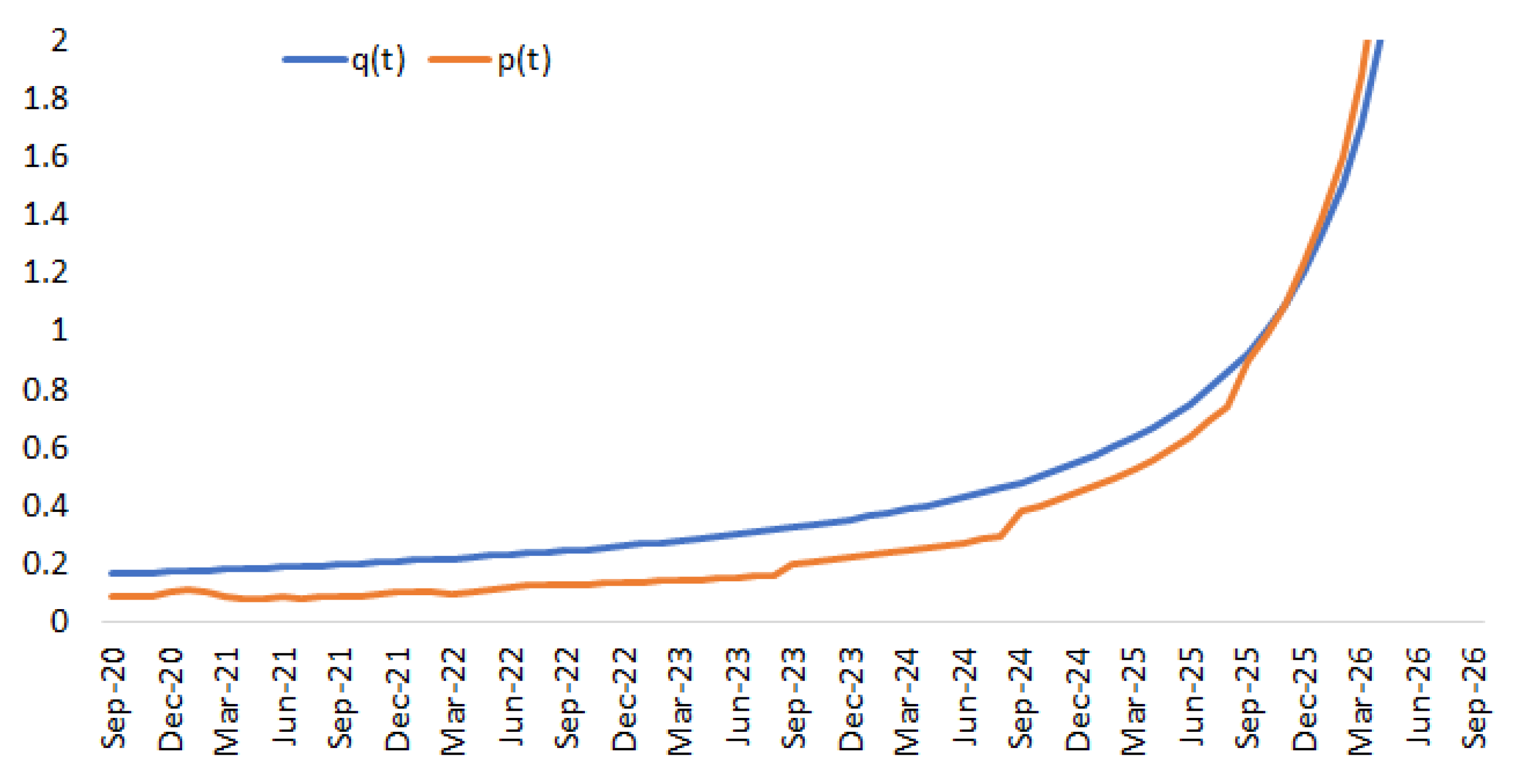
Note, in passing, that the dynamics (99) is not only one-dimensional but also resambles one typically used in the equity space to model the evolution of stock prices where the risk neutral drift of a share of stock is made up of the risk-free rate adjusted by the stock’s dividend yield. Here, in the drift term $q\left(t\right)-p\left(t\right)$, $q\left(t\right)$ can be thought of as the “short rate” and $p\left(t\right)$—the “dividend yield.” The calculation of ${sup}_{\tau \in \mathcal{T}}{\mathbb{E}}^{\mathbb{Q}}\left[\tilde{Q}\left(\tau \right){\left(K-\tilde{S}\left(\tau \right)\right)}^{+}\right]$ should now be a straightforward exercise, and can be handled either in a finite difference pricer or LSMC simulation. We favor the former approach. Concretely, we now set $T_{{\alpha }_1}=1,T_{{\beta }_1}=6$ and $T_{{\alpha }_2}=1,T_{{\beta }_2}=11$ for two sample Bermudans: a 6-nc-1 and an 11-nc-1, respectively. As above, we use USD interest rate curve and volatility data as of September 2020.

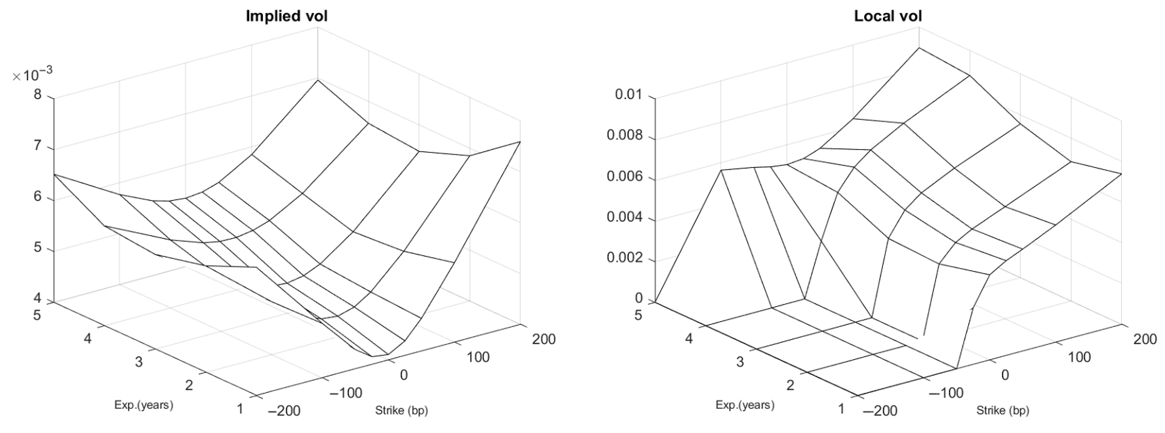
First, we calculate $p\left(t\right)$ and $q\left(t\right)$ using yield curve data which we then use—along with market prices of co-terminal swaptions—to derive the local volatility surface from the approximated PDE:

$$\sigma {(t,K)}^2\approx 2\frac{{\partial }_{t}C(t,K)-\left(q\left(t\right)-p\left(t\right)\right)K{\partial }_{K}C(t,K)+p\left(t\right)C(t,K)}{{\partial }_{KK}^{2}C(t,K)}.$$

(101)

The result of this stripping exercise is shown in Figure 7 and Figure 8.

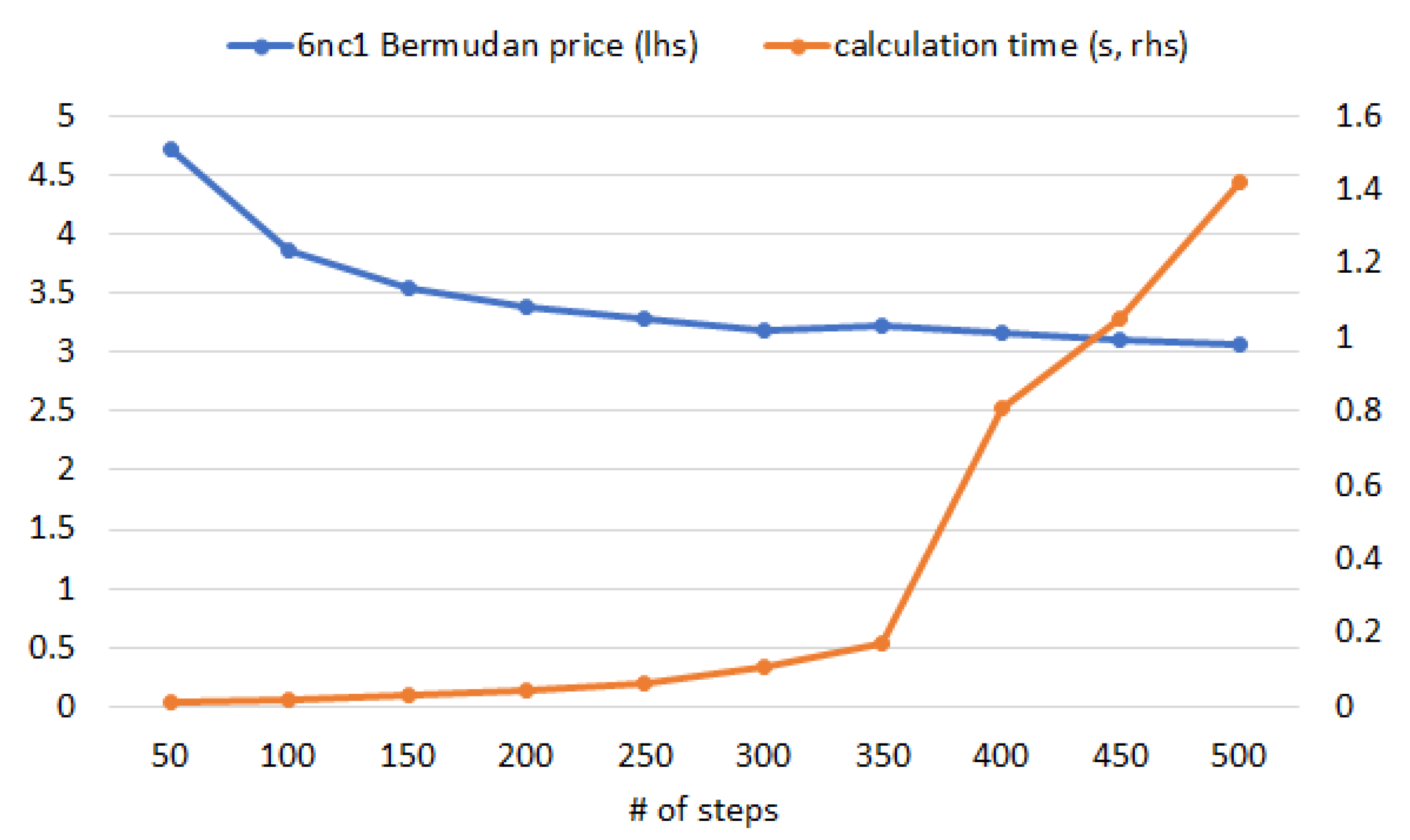
Once the local volatility has been calculated (separately for each of the swap maturity dates $T=6$ and $T=11$), we set up the finite difference grid for the process (99). In each case the boundaries are selected such that $S_{max}=E\left(S\left(T\right)\right)+4\sqrt{Var\left(S\right(T\left)\right)}$ and $S_{min}=-S_{max}$ which translate to $\pm 0.06$ for $T=6$ and $\pm 0.08$ for $T=11$. For reference, we use 400 time steps and 400 grid intervals and solve the valuation PDE using the Crank-Nicolson method with Gauss-Seidel successive overrelaxation for improved convergence. Calculation time in both cases is instantaneous (Figure 9).

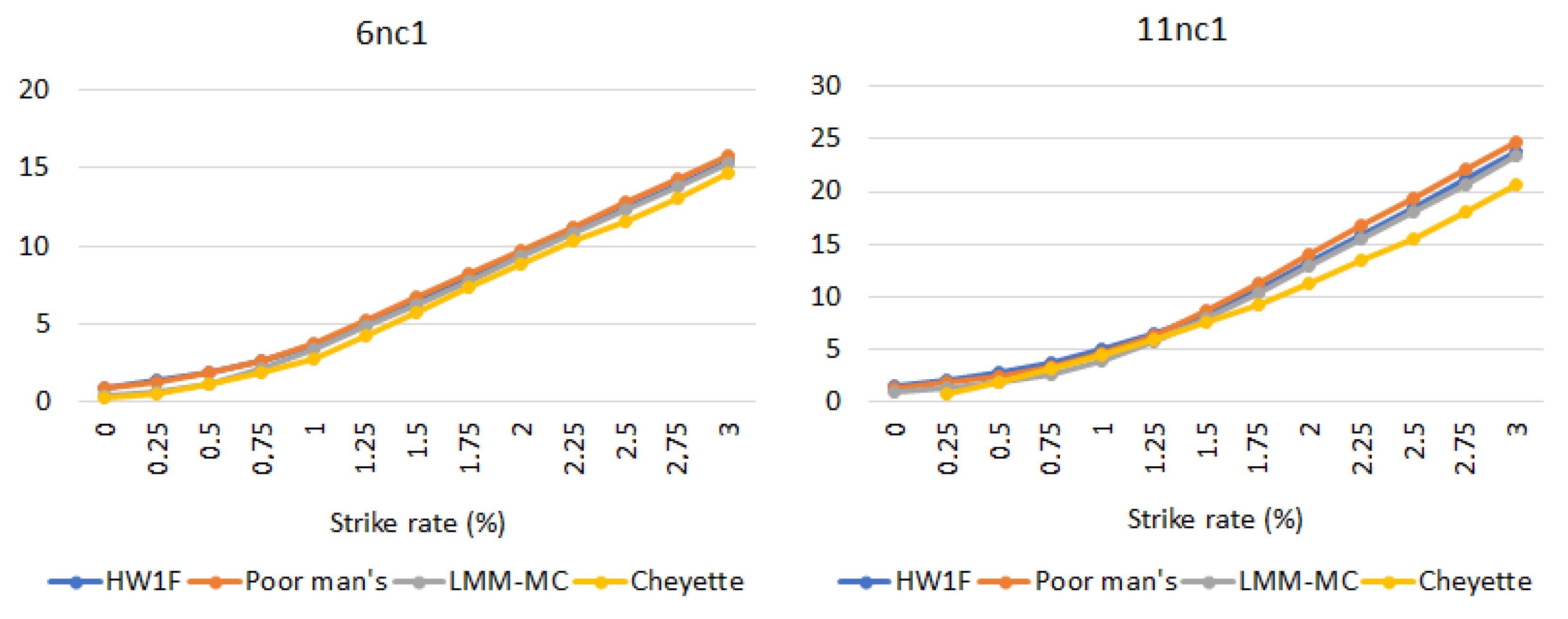
We benchmark valuation results against the whole class of models discussed above: the market standard Hull-White one-factor model, the two-factor Cheyette model, as well as the multi-factor Libor Market Model, obtaining the results shown in Figure 10.

Perhaps the first most striking observation is that the prices for strike rates ranging from 0% to 3% derived from the respective models tend to be generally closely aligned (Cheyette appears to underprice high-strike swaptions which may be due to the Monte Carlo implementation). Remarkably, the approximated model—i.e., the “poor man’s” approach, featuring an evolution of only a single process—produces results which seem to be within normal market bid-ask spreads (not to mention model-based uncertainty) of those calculated using a fully-fledged multi-factor Libor Market Model, or a local-volatility-enhanced Cheyette term structure model. As we have stressed above, the “poor man’s” model can be readily implemented in a finite difference scheme, with minimal adaptations to standard American equity option pricers, which ensures faster convergence as compared to the Cheyette Monte Carlo implementation (see again Figure 9). This demonstrates not only the fitting capability of the model, but—perhaps equally important—that Markovian projection in our extended framework can be fruitfully employed to valuing derivatives with early exercise features.

6. Conclusions

We have tried above to sketch our perspective on several decades of evolution in modeling the term structure of interest rates, with a particular focus on the travails involved in pricing Bermudan swaptions. While our treatment is by no means exhaustive, we hope to have shed light on the fascinating “tug of war” between the pursuit of calibration and pricing precision, tractability and implementation efficiency. The curse of dimensionality presented with recourse to Greek mythology boils down to the fact that the exercise boundary between the continuation area and stopping area is inherently complex and multi-dimensional for interest rate products. Ironically, therefore, the better we can capture and describe the product itself (i.e., the more factors we use), the poorer and less exact our handle on the exercise boundary is. And yet, we believe that our extension of the classic approach due to Gyöngy [28] promises a potentially attractive way past both the “Scylla” and “Charybdis” paths. Specifically, on the theoretical side, we show that it is possible to construct a process that mimics the discounted marginal distributions of a given Ito process, but is considerably simpler in the sense that its drift and diffusion terms are non-random, localized versions of the drift and diffusion of the original process (which in general may themselves be stochastic processes). This means that for purposes of swaption pricing, a potentially complex and multidimensional process for the underlying swap rate can be collapsed to a one-dimensional one. The empirical contribution complementing our theoretical observation consists in demonstrating that even though we only match the marginal distributions of the two processes, Bermudan swaption prices calculated using such an approach appear well-behaved and closely aligned to counterparts from more sophisticated models. And while much remains to be done in this area—not least in understanding what exactly enforces the alignment between the true early exercise boundary and the approximated ones—we believe that Markovian projection can be further fruitfully exploited in pricing interest rate products with early exercise features.

References

- Guenther, R.; Lee, J. Heat conduction with radiating boundary conditions. J. Comput. Appl. Math. 1998, 88, 119–124. [Google Scholar] [CrossRef] [Green Version]
- Kuske, R.A.; Keller, J.B. Optimal exercise boundary for an American put option. Appl. Math. Financ. 1998, 5, 107–116. [Google Scholar] [CrossRef]
- Barles, G.; Burdeau, J.; Romano, M.; Samsoen, N. Critical stock price near expiration. Math. Financ. 1995, 5, 77–95. [Google Scholar] [CrossRef]
- Black, F.; Scholes, M. The pricing of options and corporate liabilities. J. Political Econ. 1973, 81, 637–654. [Google Scholar] [CrossRef] [Green Version]
- Geman, H.; Karoui, N.E.; Rochet, J.-C. Changes of numeraire, changes of probability measure and option pricing. J. Appl. Probab. 1995, 32, 443–458. [Google Scholar] [CrossRef]
- Andersen, L.; Piterbarg, V. Interest Rate Modelling Volume; Atlantic Financial Press: London, UK, 2010. [Google Scholar]
- Interest Rate Models-Theory and Practice: With Smile, Inflation and Credit; Springer Science & Business Media: Berlin/Heidelberg, Germany, 2007.
- Vasicek, O. An equilibrium characterization of the term structure. J. Financ. Econ. 1977, 5, 177–188. [Google Scholar] [CrossRef]
- Longstaff, F.A.; Santa-Clara, P.; Schwartz, E.S. Throwing away a billion dollars: The cost of suboptimal exercise strategies in the swaptions market. J. Financ. Econ. 2001, 62, 39–66. [Google Scholar] [CrossRef]
- Brace, A.; Gatarek, D.; Musiela, M. The market model of interest rate dynamics. Math. Financ. 1997, 7, 127–155. [Google Scholar] [CrossRef] [Green Version]
- Jamshidian, F. LIBOR and swap market models and measures. Financ. Stochastics 1997, 1, 293–330. [Google Scholar] [CrossRef] [Green Version]
- Miltersen, K.R.; Sandmann, K.; Sondermann, D. Closed form solutions for term structure derivatives with log-normal interest rates. J. Financ. 1997, 52, 409–430. [Google Scholar] [CrossRef]
- Andersen, L.; Andreasen, J. Volatility skews and extensions of the Libor market model. Appl. Math. Financ. 2000, 7, 1–32. [Google Scholar] [CrossRef]
- Brigo, D.; Mercurio, F. Analytical pricing of the smile in a forward LIBOR market model. Quant. Financ. 2003, 3, 15–27. [Google Scholar] [CrossRef]
- Zühlsdorff, C. Extended Libor Market Models with Affine and Quadratic Volatility; Verlag Dr. Kovac: Hamburg, Germany, 2002. [Google Scholar]
- Andersen, L.B.; Brotherton-Ratcliffe, R. Extended Libor Market Models with Stochastic Volatility. J. Comput. Financ. 2005, 9. [Google Scholar] [CrossRef]
- Joshi, M.S.; Rebonato, R. A displaced-diffusion stochastic volatility LIBOR market model: Motivation, definition and implementation. Quant. Financ. 2003, 3, 458–469. [Google Scholar] [CrossRef]
- Piterbarg, V.V. Stochastic Volatility Model with Time-dependent Skew. Appl. Math. Financ. 2005, 12, 147–185. [Google Scholar] [CrossRef]
- Wu, L.; Zhang, F. The stochastic volatility Libor market model. Risk 2001, 14, 105–109. [Google Scholar] [CrossRef]
- Wu, L.; Zhang, F. Libor market model with stochastic volatility. J. Ind. Manag. Optim. 2006, 2, 199. [Google Scholar] [CrossRef]
- LIBOR Market Model with Semimaringales. In Handbooks in Mathematical Finance, Topics in Option Pricing, Interest Rates and Risk Management; Cambridge University Press: Cambridge, UK, 2001.
- Jarrow, R.; Li, H.; Zhao, F. Interest rate caps “smile” too! but can the Libor market models capture the smile? J. Financ. 2007, 62, 345–382. [Google Scholar] [CrossRef]
- Andersen, L.; Andreasen, J. Factor dependence of bermudan swaptions: Fact or fiction? J. Financ. Econ. 2001, 62, 3–37. [Google Scholar] [CrossRef]
- Gatarek, D. Pricing of American swaptions in approximate lognormal model. In University of New South Wales Working Paper; University of New South Wales: Sydney, Australia, 1996. [Google Scholar]
- Longstaff, F.A.; Schwartz, E.S. Valuing American options by simulation: A simple least-squares approach. Rev. Financ. Stud. 2001, 14, 113–147. [Google Scholar] [CrossRef] [Green Version]
- Glasserman, P. Monte Carlo Methods in Financial Engineering; Springer Science & Business Media: Berlin/Heidelberg, Germany, 2013; Volume 53. [Google Scholar]
- Towards a general local volatility model for all asset classes. J. Deriv. 2019, 27, 14–30. [CrossRef]
- Gyöngy, I. Mimicking the one-dimensional marginal distributions of processes having an Itô differential. Probab. Theory Relat. Fields 1986, 71, 501–516. [Google Scholar] [CrossRef]
- Dupire, B. Pricing with a smile. Risk 1994, 7, 18–20. [Google Scholar]
- Hull, J.; White, A. Pricing interest-rate-derivative securities. Rev. Financ. Stud. 1990, 3, 573–592. [Google Scholar] [CrossRef]
- Boyle, P.P. Immunization under stochastic models of the term structure. J. Inst. Actuar. (1886–1994) 1978, 105, 177–187. [Google Scholar] [CrossRef] [Green Version]
- Black, F.; Karasinski, P. Bond and option pricing when short rates are lognormal. Financ. Anal. J. 1991, 47, 52–59. [Google Scholar] [CrossRef]
- Cheyette, O. Term structure dynamics and mortgage valuation. J. Fixed Income 1992, 1, 28–41. [Google Scholar] [CrossRef]
- Hull, J.C.; White, A.D. Numerical procedures for implementing term structure models II: Two-factor models. J. Deriv. 1994, 2, 37–48. [Google Scholar] [CrossRef]
- Ritchken, P.; Sankarasubramanian, L. Volatility structures of forward rates and the dynamics of the term structure1. Math. Financ. 1995, 5, 55–72. [Google Scholar] [CrossRef]
- Gatarek, D.; Jabłecki, J.; Qu, D. Non-parametric local volatility formula for interest rate swaptions. Risk 2016, 20, 120–124. [Google Scholar]
- Andreasen, J. Turbo Charging the Cheyette Model (1 June 2001). Available online: https://ssrn.com/abstract=1719142 (accessed on 5 January 2021).
- Chibane, M.; Law, D. A quadratic volatility Cheyette model. Risk 2013, 7, 68–71. [Google Scholar] [CrossRef]
- Gatarek, D.; Jabłecki, J. A nonparametric local volatility model for swaptions smile. J. Comput. Financ. 2018, 21, 35–62. [Google Scholar] [CrossRef]
- Heath, D.; Jarrow, R.; Morton, A. Bond pricing and the term structure of interest rates: A new methodology for contingent claims valuation. Econom. J. Econom. Soc. 1992, 77–105. [Google Scholar] [CrossRef]
- Qu, D. Manufacturing and Managing Customer-Driven Derivatives; John Wiley & Sons: Chichester, UK, 2016. [Google Scholar]
- Anonymous. Back to the future. Risk 2005, 104–109. [Google Scholar]
- Morini, M. Understanding and Managing Model Risk: A Practical Guide for Quants, Traders and Validators; John Wiley & Sons: Hoboken, NJ, USA, 2011. [Google Scholar]
- Volatility and Correlation: The Perfect Hedger and the Fox; John Wiley & Sons: Hoboken, NJ, USA, 2005.
- Gatarek, D. Modelling without tears. Risk 2000, 20–24. [Google Scholar]
- Gatarek, D.; Bachert, P.; Maksymiuk, R. The LIBOR Market Model in Practice; John Wiley & Sons: Hoboken, NJ, USA, 2007; Volume 408. [Google Scholar]
- Hagan, P.S. Methodology for Callable Swaps and Bermudan “Exercise into” Swaptions; Discussion Paper; Bloomberg: New York, NY, USA, 2000. [Google Scholar]
- Tavella, D.; Randall, C. Pricing Financial Instruments: The Finite Difference Method; John Wiley & Sons: Hoboken, NJ, USA, 2000; Volume 13. [Google Scholar]
- Mitchell, A.R.; Griffiths, D.F. The Finite Difference Method in Partial Differential Equations; Wiley: Hoboken, NJ, USA, 1980. [Google Scholar]
- Hull, J.C.; White, A.D. Numerical procedures for implementing term structure models I: Single-factor models. J. Deriv. 1994, 2, 7–16. [Google Scholar] [CrossRef]
- Craig, I.J.; Sneyd, A.D. An alternating-direction implicit scheme for parabolic equations with mixed derivatives. Comput. Math. Appl. 1988, 16, 341–350. [Google Scholar] [CrossRef] [Green Version]
- Tilley, J.A. Valuing American options in a path simulation model. Trans. Soc. Actuar. 1993, 45, 83–104. [Google Scholar]
- Carriere, J.F. Valuation of the early-exercise price for options using simulations and nonparametric regression. Insur. Math. Econ. 1996, 19, 19–30. [Google Scholar] [CrossRef]
- Glasserman, P.; Yu, B. Number of paths versus number of basis functions in American option pricing. Ann. Appl. Probab. 2004, 14, 2090–2119. [Google Scholar]
- Jackel, P.; Rebonato, R. The link between caplet and swaption volatilities in a Brace-Gatarek-Musiela/Jamshidian framework: Approximate solutions and empirical evidence. J. Comput. Financ. 2003, 6, 41–60. [Google Scholar] [CrossRef]
- Rebonato, R. Interest Rate Options Models; Wiley: Hoboken, NJ, USA, 1998. [Google Scholar]
- Lvov, D.N. Monte Carlo Methods for Pricing and Hedging: Applications to Bermudan Swaptions and Convertible Bonds. Ph.D. Thesis, ISMA Centre University of Reading, Reading, UK, 2005. [Google Scholar]
- Svenstrup, M. On the suboptimality of single-factor exercise strategies for Bermudan swaptions. J. Financ. Econ. 2005, 78, 651–684. [Google Scholar] [CrossRef] [Green Version]
- Gatarek, D.; Jabłecki, J. Swap Rate à la Stock: Bermudan Swaptions Made Easy. Wilmott 2020, 2020, 44–51. [Google Scholar] [CrossRef]
Figure 1.
The distribution of Vega risk across maturity and tenor buckets for a 21nc1 receiver ATM Bermudan swaption (in % of total swaption Vega).
Figure 2.
Price of a 11nc1 Bermudan receiver swaption plotted against the prices of co-terminal Europeans (all options struck at ).
Figure 3.
The 21nc1 Bermudan swaption and its most expensive Europeans in different market regimes.
Figure 4.
Comparison of “20-non-call-10” Bermudan swaption prices calculated with a one-factor Hull–White model using a finite difference scheme and Least Square Monte Carlo (in percent; USD market data as of September 2020). Note: for reference, the LSMC uses 25,000 presimulation paths to fit the coefficients and then another 25,000 with antithetic variates (a total of 50,000 paths) to estimate continuation values based on the previously determined decision rule; we used twelve time steps per year and standard Euler discretization; the Crank–Nicolson finite difference gird has a resolution of 20 time steps per year and 400 space steps.
Figure 5.
Factor dependence: prices of Bermudan swaptions on 5Y (left-hand panel) and 10Y swaps (right-hand panel) with time to first exercise set at 1, 5 and 10 years calculated using single- and multi-factor models calibrated to USD market data as of 11 September 2020 (in percent).
Figure 6.
Prices of 20-nc-10 Bermudan swaption in a full-factor LIBOR market model under different base correlation assumptions.
Figure 7.
Implied volatility surface and its corresponding local volatility surface stripped using (101). Note: Terminal swap maturity is fixed at 6 years; US market data as of 28 September 2020; to avoid “sinkholes” local volatility floored at zero.
Figure 8.
“Short-rate-like” and “dividend-like” parameters and of the process (99) (stripped from yield curve data as of 28 September 2020). Note: and , ; plot truncated due to explosive behavior of p with ;
Figure 9.
Convergence profile of the Crank-Nicolson scheme implemented for the 6nc1 Bermudan swaption.
Figure 10.
Model prices of a 6nc1 (lhs panel) and 11nc1 (rhs panel) Bermudan receiver swaptions with 100 notional.
Publisher’s Note: MDPI stays neutral with regard to jurisdictional claims in published maps and institutional affiliations. |
© 2021 by the authors. Licensee MDPI, Basel, Switzerland. This article is an open access article distributed under the terms and conditions of the Creative Commons Attribution (CC BY) license (http://creativecommons.org/licenses/by/4.0/).
Share and Cite
MDPI and ACS Style
Gatarek, D.; Jabłecki, J. Between Scylla and Charybdis: The Bermudan Swaptions Pricing Odyssey. Mathematics 2021, 9, 112. https://0-doi-org.brum.beds.ac.uk/10.3390/math9020112
AMA Style
Gatarek D, Jabłecki J. Between Scylla and Charybdis: The Bermudan Swaptions Pricing Odyssey. Mathematics. 2021; 9(2):112. https://0-doi-org.brum.beds.ac.uk/10.3390/math9020112
Chicago/Turabian StyleGatarek, Dariusz, and Juliusz Jabłecki. 2021. "Between Scylla and Charybdis: The Bermudan Swaptions Pricing Odyssey" Mathematics 9, no. 2: 112. https://0-doi-org.brum.beds.ac.uk/10.3390/math9020112
Note that from the first issue of 2016, this journal uses article numbers instead of page numbers. See further details here.