Bayesian Inference under Small Sample Sizes Using General Noninformative Priors

Abstract

This paper proposes a Bayesian inference method for problems with small sample sizes. A general type of noninformative prior is proposed to formulate the Bayesian posterior. It is shown that this type of prior can represent a broad range of priors such as classical noninformative priors and asymptotically locally invariant priors and can be derived as the limiting states of normal-inverse-Gamma conjugate priors, allowing for analytical evaluations of Bayesian posteriors and predictors. The performance of different noninformative priors under small sample sizes is compared using the likelihood combining both fitting and prediction performances. Laplace approximation is used to evaluate the likelihood. A realistic fatigue reliability problem was used to illustrate the method. Following that, an actual aeroengine disk lifing application with two test samples is presented, and the results are compared with the existing method.

1. Introduction

Sample sizes are often quite small in many engineering fields due to time, economic, and physical constraints, for example, life testing data of high-reliability mechanical components, large and complex engineering systems, and so on. The influence of sample size on interpreting classical significance test results has been discussed in several studies [1,2,3]. The predictive models established based on scarce samples may highly depend on the chosen parameter estimation method [4,5]. In those cases, the probabilistic approach is usually preferred over the deterministic approach [6,7,8,9,10,11]. The Bayes rule provides a consistent and rational mathematical device to incorporate relevant information and prior knowledge for probabilistic inference.

To motivate the discussion, consider an observable random variable X with a conditional probability density function (PDF) (or simply density) of $p\left(x\right|\varphi )$, where $\varphi \in \Phi$ is also a random variable. The inverse problem is to make inferences about $\varphi$ given an observed value x of X. The Bayesian approach to the solution is to use some density $p\left(\varphi \right)$ over $\Phi$ to represent the prior information of $\varphi$. In this way, the prior knowledge of $\varphi$ can be encoded through the Bayes rule to obtain the posterior PDF of $\varphi$ given x,

$$p\left(\varphi \right|x)\propto p(\varphi \left)p\right(x\left|\varphi \right).$$

(1)

The forward inference, e.g., the PDF of a certain variable or the probability of an event involving $\varphi$, can be made on the basis of the posterior PDF. Using the method of Markov chain Monte Carlo (MCMC), samples can directly be drawn from the posterior distribution without knowing the normalizing constant $p\left(x\right)=\int p\left(\varphi \right)p\left(x\right|\varphi )\mathrm{d}\varphi$ in Equation (1). The Bayesian method has been successfully demonstrated in all important disciplines [12,13,14,15,16,17,18,19].

The choice of $p\left(\varphi \right)$ can have a great influence on the inference result. The proper choice of priors has been extensively discussed in the probability and statistics communities, and it can never be overlooked as it is one of the fundamental pieces of Bayesian inference [20,21,22,23,24,25,26]. For one thing, the formal rule of constructing a prior regardless of the data and likelihood is sought in the field of physics [9,27]. Jaynes and Bretthorst [28] argued that “problems of inference are ill-posed until we recognize three essential things. (A) The prior probabilities represent our prior information, and are to be determined, not by introspection but by logical analysis of that information. (B) Since the final conclusions depend necessarily on both the prior information and the data, it follows that, in formulating a problem, one must specify the prior information to be used just as fully as one specifies the data. (C) Our goal is that inferences are to be completely ‘objective’ in the sense that two persons with the same prior information must assign the same prior probabilities.” (p. 373). For another, the choice of a prior may highly depend on data and likelihood in practice. Gelman et al. [29] argued that “a prior can in general only be interpreted in the context of the likelihood with which it will be paired” (p. 12).

To ensure a consistent and objective inference, rules for constructing priors with minimal subjective constraints are sought. Early work on the construction of such priors is based on the “ignorance” over the parameter space using invariance techniques [27,30,31]. The fundamental reasoning is that the priors should carry the same amount of information such that a change of scale and/or a shift of location do not affect the inference results on those parameters. The ignorant prior can systematically be derived using the concept of the transformation group. Using different transformation groups, different priors can be obtained. For simplicity, such priors are loosely referred to as noninformative priors. One of the most notable priors for a scale parameter $\sigma$ of a distribution is Jeffreys’ prior, i.e., $p\left(\sigma \right)\propto 1/\sigma$. Jeffreys’ prior can be obtained using the tool of the transformation group under the condition that a change of scale does not change that state of knowledge. A further extension of the noninformative priors is “reference priors” [32,33]. The theoretical framework has been discussed in many studies, including, but not limited to, [31,34]. Apart from the noninformative approach to derive the priors, there are several less objective approaches to construct the priors. Gelman [35] proposed the weakly informative priors based on the idea of conditional conjugacy for hierarchical Bayesian models. The conditionally conjugate priors provide some computational convenience as a Gibbs sampler can be used to draw samples from a posterior distribution, and some parameters for inverse-Gamma distributions in Bayesian applications are suggested. Simpson et al. [36] proposed a method to build priors. The basic idea is to penalize the complexity induced by deviating from a simpler base model using the Kullback–Leibler divergence as a metric [37].

For critical problems with small sample sizes, the choice of the prior in Bayesian inference can have a great impact on the inference results, rendering an unreliable decision-making. Despite a great deal of research, including the aforementioned, having been conducted, the choice of an optimal prior is still nontrivial to make from the practical point of view, and a systematical method to cope with such cases is rarely seen. Moreover, a quantitative measure to evaluate the performance of a prior is equally important to identify the optimal prior. This study develops a noninformative Bayesian approach to probabilistic inference under small sample sizes. A general $1/{\sigma }^q$-type of noninformative prior for the location-scale family of distributions is proposed. This type of prior is further shown to be the limiting state of the commonly used normal-inverse-Gamma conjugate prior, thus allowing for an analytical evaluation of the posterior of the parameter. Given a linear model with a Gaussian error variable, the analytical form of the posterior of the model prediction can also be obtained. The informative or noninformative nature of the prior is centered more on the concept of whether the prior encodes subjective information; therefore, it is less relevant to the likelihood function (and data). The subjective information is the source of inconsistency in the inference result as different practitioners can use different subjective information in the form of assumptions, which in most cases may only be justified by oneself. However, the prior has to be built with a certain state of knowledge. This state of knowledge, or loosely called information, is not related to experience nor assumptions, but is a result of a logical reasoning process [27]. The purpose of the study is not to argue whether these assumptions are justified or not, nor to question the suitable assumptions made during the inference. This study provides an alternative to existing methods in such cases to avoid introducing subjectiveness into the Bayesian inference. In particular, when the number of samples is small, the influence of the prior can be as important as the likelihood (and data). In such cases, subjective information encoded in the prior can lead to biased results.

The remainder of the paper is organized as follows. First, the Bayesian model with noninformative priors is developed, in particular, a general $1/{\sigma }^q$-type of noninformative prior for the location-scale family of distributions is proposed for small sample problems. The noninformative priors are further shown as the limiting states of the normal-inverse-Gamma (NIG) conjugate priors. The closed-form expressions of the Bayesian posterior and predictors using the proposed noninformative priors are obtained under a Gaussian likelihood. Next, a performance measure considering both the fitting performance and predictive performance is proposed using the concept of Bayes factors. Different priors are treated as models in a Bayesian hypothesis testing context for comparisons. Following that, the method is illustrated using two examples.

2. Bayesian Linearized Models with Noninformative Priors

To motivate the discussion, consider a general linear or linearized model:

$$y_i={\mathbf{x}}_i\theta +{ϵ}_i,$$

(2)

where $\theta$ is a k-dimensional column vector and ${ϵ}_i$ are independent and identical distributed random error variables. The distribution of ${ϵ}_i$ determines the likelihood function or vice versa. Without loss of generality, the distribution belongs to a location-scale family of distributions. Furthermore, it is enough to use a single scale parameter to characterize the distribution of $ϵ$ since any constant nonzero mean, no matter known or unknown, can be grouped into $\theta$. Denote the scale parameter of $ϵ$ as ${\sigma }^2$. A Bayesian model incorporates both the prior information and the observation through Bayes’ rule. Using the matrix form $\mathbf{y}=\mathbf{x}\theta +ϵ$, the Bayesian posterior of $(\theta ,{\sigma }^2)$ writes:

$$p(\theta ,{\sigma }^2|\mathbf{y})\propto p(\theta ,{\sigma }^2)p\left(\mathbf{y}\right|\theta ,{\sigma }^2).$$

(3)

The common Gaussian error variable, i.e., ${ϵ}_i\sim N(0,{\sigma }^2)$, corresponds to the following likelihood function, for n observations $\mathbf{y}={(y_1,y_2,\dots ,y_n)}^T$ and n input vector $\mathbf{x}={({\mathbf{x}}_1,{\mathbf{x}}_2,\dots ,{\mathbf{x}}_n)}^T$ where ${\mathbf{x}}_i$, $i=1,\dots ,n$, is a row vector of size k.

$$\begin{array}{cc}\hfill p\left(\mathbf{y}\right|\theta ,{\sigma }^2)& =\mathrm{N}(\mathbf{x}\theta ,{\sigma }^2\mathrm{I})\hfill \\ \hfill & \propto {\sigma }^{-n}exp\left[{\displaystyle -\frac{1}{2{\sigma }^2}\sum _{i=1}^n{\left(y_i-{\mathbf{x}}_i\theta \right)}^2}\right].\hfill \end{array}$$

(4)

It should be noted that the error variable does not necessarily follow a Gaussian PDF, and other types of error distributions can be used. For example, the extreme-value PDF for the error corresponds to a Weibull likelihood for the log-transformed model prediction.

2.1. A General Form of Noninformative Priors—$\propto 1/{\sigma }^q$

A general $\propto 1/{\sigma }^q$ ($q>=0$) form of priors is considered here. The classical Jeffreys’ prior and the related asymptotically locally invariant priors are introduced first for the purpose of completeness.

Consider the PDF of a random variable x characterized by a parameter vector $\varphi$; Jeffreys’ noninformative prior distribution of $\varphi$ is proportional to the square root of the determinant of the Fisher information matrix, e.g.,

$$p\left(\varphi \right)\propto \sqrt{\det \mathbf{I}(\varphi )},$$

(5)

where $\det (·)$ is the determinant operator and $\mathbf{I}(·)$ is the Fisher information matrix. The key feature of it is invariance under the monotone transformation of $\varphi$. This feature is achieved by using the change of variables theorem. Denote the reparameterized variable or vector as $\psi$; it can be shown that:

$${\displaystyle p\left(\psi \right)=p\left(\varphi \right)\left|\det \frac{\partial {\varphi }_i}{\partial {\psi }_j}\right|=\sqrt{\det \mathbf{I}\left(\psi \right)},}$$

(6)

For a Gaussian likelihood with unknown parameters $\mathsf{\mu }$ and ${\sigma }^2$,

$$p\left(x\right|\mathsf{\mu },{\sigma }^2)=\frac{1}{\sqrt{2\pi {\sigma }^2}}exp\left[-\frac{{(x-\mathsf{\mu })}^2}{2{\sigma }^2}\right].$$

(7)

Jeffreys’ prior for the joint parameter $(\mathsf{\mu },{\sigma }^2)$ is:

$$p(\mathsf{\mu },{\sigma }^2)\propto \sqrt{\det \mathbf{I}(\mathsf{\mu },{\sigma }^2)},$$

(8)

where $\mathbf{I}(\mathsf{\mu },{\sigma }^2)$ is:

$$\mathbf{I}=\mathbb{E}\left[\begin{array}{ccc}{\displaystyle \frac{\partial lnp\left(x\right|·)}{\partial \mathsf{\mu }}}{\displaystyle \frac{\partial lnp\left(x\right|·)}{\partial \mathsf{\mu }}}& & {\displaystyle \frac{\partial lnp\left(x\right|·)}{\partial \mathsf{\mu }}}{\displaystyle \frac{\partial lnp\left(x\right|·)}{\partial \left({\sigma }^2\right)}}\\ {\displaystyle \frac{\partial lnp\left(x\right|·)}{\partial \mathsf{\mu }}}{\displaystyle \frac{\partial lnp\left(x\right|·)}{\partial \left({\sigma }^2\right)}}& & {\displaystyle \frac{\partial lnp\left(x\right|·)}{\partial \left({\sigma }^2\right)}}{\displaystyle \frac{\partial lnp\left(x\right|·)}{\partial \left({\sigma }^2\right)}}\end{array}\right]$$

(9)

and $\mathbb{E}(·)$ is the expectation operator. Using algebraic deduction and integration, $\mathbf{I}(\mathsf{\mu },{\sigma }^2)$ is simplified to:

$$\mathbf{I}=\left[\begin{array}{ccc}{\displaystyle \frac{1}{{\sigma }^2}}& & 0\\ 0& & {\displaystyle \frac{2}{{\sigma }^4}}\end{array}\right].$$

(10)

As a result, Jeffreys’ prior for $(\mathsf{\mu },{\sigma }^2)$ is:

$$p(\mathsf{\mu },{\sigma }^2)\propto 1/{\sigma }^3.$$

(11)

It is noted that the distribution of interest is $(\mathsf{\mu },{\sigma }^2)$, not $(\mathsf{\mu },\sigma )$; therefore, the derivative is taken with respective to ${\sigma }^2$ as a whole instead of $\sigma$. In other word, the parameter space is on ${\sigma }^2$, not $\sigma$. For example, the Jeffreys’ prior for ${\sigma }^2$, with a fixed value of $\mathsf{\mu }$, is:

$$p\left({\sigma }^2\right)\propto \frac{1}{{\sigma }^2}.$$

(12)

The Jeffreys’ prior for $(\mathsf{\mu },\sigma )$ and $\sigma$ with a fixed $\mathsf{\mu }$ are $\propto 1/{\sigma }^2$ and $\propto 1/\sigma$, respectively. It is shown in Appendix B that the Fisher information matrix is also the Hessian matrix of the Kullback–Leibler (KL) distance of a deviated distribution with respect to the true distribution evaluated at the true parameters. For exponential families of distributions, the KL distance has analytical forms, allowing for the evaluation of the Fisher information matrix without involving integrals in Equation (9).

The asymptotically locally invariant (ALI) prior is another type of prior that satisfies the invariance under certain transformations. An ALI prior can be uniquely determined using the following equation according to [31],

$$\frac{\partial lnp\left(\varphi \right)}{\partial \varphi }=-\mathbb{E}\left[f_1{f}_2\right]/\mathbb{E}\left[f_2\right],$$

(13)

where $f_1=\partial lnp\left(x\right|·)/\partial \varphi$ and $f_2={\partial }^{2}lnp\left(x\right|·)/\partial {\varphi }^2$. For a Gaussian distribution with a fixed mean and a random $\sigma$, the two terms are $\mathbb{E}\left[f_1{f}_2\right]=-6/{\sigma }^3$ and $\mathbb{E}\left[f_2\right]=-2/{\sigma }^2$. Solve:

$$\frac{\partial lnp\left(\sigma \right)}{\partial \sigma }=-\frac{3}{\sigma }$$

(14)

to obtain the ALI prior for $\sigma$:

$$p\left(\sigma \right)\propto \frac{1}{{\sigma }^3}.$$

(15)

Similarly, the ALI prior for ${\sigma }^2$ is:

$$p\left({\sigma }^2\right)\propto \frac{1}{{\sigma }^4}.$$

(16)

When both $\mathsf{\mu }$ and $\sigma$ are random, the joint ALI prior for $(\mathsf{\mu },\sigma )$ is:

$$p(\mathsf{\mu },\sigma )\propto \frac{1}{{\sigma }^5}.$$

(17)

It is noticed that the Jeffreys’, ALI, and uniform priors are reproduced from $\propto 1/{\sigma }^q$ as q takes different integer values. In the following, the derivation of a $1/{\sigma }^q$ prior from NIG conjugates is shown.

2.2. Derivation of the $1/{\sigma }^q$ Priors as the Limiting States of NIG Conjugates under Gaussian Likelihood

In Bayesian models, for the given likelihood function, the posterior $p\left(\varphi \right|x)$ and the prior $p\left(\varphi \right)$ are called conjugate distributions if both are in the same family of distributions. It can be considered as the prior can be reconditioned by encoding the evidence through the likelihood; therefore, the evidence or data merely change the distribution parameters of the prior and yield another distribution of the same type, but with a different set of parameters.

For a location-scale parameter vector $(\theta ,{\sigma }^2)$ used in linear or linearized Bayesian models with a Gaussian likelihood, the corresponding conjugate prior is the NIG distribution. The closed-form posterior PDFs for the parameter and prediction are given in Appendix A.

Noninformative priors, including the Jeffreys’, ALI, and reference priors, for $(\theta ,{\sigma }^2)$ are mostly in the form of $1/{\sigma }^q$, $q\in 1,2,\dots$. The uniform prior can be seen as a special case of $1/{\sigma }^q$ as $q=0$. It is shown as follows that these noninformative priors can be obtained as certain limiting states of NIG conjugates of $(\theta ,{\sigma }^2)$. For example, the NIG distribution with parameters $(\alpha ,\beta ,\Sigma ,\mathsf{\mu })$ given by Equation (A3) can reduce to the Jeffreys’ prior:

$$p(\theta ,{\sigma }^2)\to \frac{1}{{\sigma }^2}$$

(18)

as:

$$\left\{\begin{array}{cc}\hfill \alpha & \to -k/2\hfill \\ \hfill \beta & \to 0^{+}\hfill \\ \hfill {\Sigma }^{-1}& \to \mathbf{0}\hfill \\ \hfill \left|\mathsf{\mu }\right|& <\infty \hfill \end{array}\right..$$

(19)

Furthermore, a $1/{\sigma }^q$-type of prior can all be derived as reduced NIG distributions. By assigning the initial values for $\alpha$, $\beta$, and $\Sigma$ of the NIG distribution, different q values are obtained.

Table 1. $1/{\sigma }^q$-type of prior as limiting state cases of the NIG distribution and its NIG posteriors.

Prior $(\mathit{\theta },{\mathit{\sigma }}^2)$	NIG$(\mathit{\alpha },\mathit{\beta },\mathit{\theta },{\mathit{\sigma }}^2)\to$ Prior	Posterior → NIG$({\mathit{\alpha }}^{\ast },{\mathit{\beta }}^{\ast },\mathit{\theta },{\mathit{\sigma }}^2)$
flat	$\begin{array}{cc}\hfill \alpha & =-k/2-1\hfill \\ \hfill \beta & \to 0\hfill \\ \hfill {\Sigma }^{-1}& \to 0\hfill \end{array}$	$\begin{array}{cc}\hfill {\alpha }^{\ast }& =\alpha +n/2=(n-k-2)/2\hfill \\ \hfill {\beta }^{\ast }& =\beta +\mathrm{SSE}/2=\mathrm{SSE}/2\hfill \\ \hfill {\Sigma }^{\ast }& ={\left({\Sigma }^{-1}+{\mathbf{x}}^T\mathbf{x}\right)}^{-1}={\left({\mathbf{x}}^T\mathbf{x}\right)}^{-1}\hfill \end{array}$
$\frac{1}{\sigma }$	$\begin{array}{cc}\hfill \alpha & =-k/2-1/2\hfill \\ \hfill \beta & \to 0\hfill \\ \hfill {\Sigma }^{-1}& \to 0\hfill \end{array}$	$\begin{array}{cc}\hfill {\alpha }^{\ast }& =\alpha +n/2=(n-k-1)/2\hfill \\ \hfill {\beta }^{\ast }& =\beta +\mathrm{SSE}/2=\mathrm{SSE}/2\hfill \\ \hfill {\Sigma }^{\ast }& ={\left({\Sigma }^{-1}+{\mathbf{x}}^T\mathbf{x}\right)}^{-1}={\left({\mathbf{x}}^T\mathbf{x}\right)}^{-1}\hfill \end{array}$
$\frac{1}{{\sigma }^2}$	$\begin{array}{cc}\hfill \alpha & =-k/2\hfill \\ \hfill \beta & \to 0\hfill \\ \hfill {\Sigma }^{-1}& \to 0\hfill \end{array}$	$\begin{array}{cc}\hfill {\alpha }^{\ast }& =\alpha +n/2=(n-k)/2\hfill \\ \hfill {\beta }^{\ast }& =\beta +\mathrm{SSE}/2=\mathrm{SSE}/2\hfill \\ \hfill {\Sigma }^{\ast }& ={\left({\Sigma }^{-1}+{\mathbf{x}}^T\mathbf{x}\right)}^{-1}={\left({\mathbf{x}}^T\mathbf{x}\right)}^{-1}\hfill \end{array}$
$\frac{1}{{\sigma }^3}$	$\begin{array}{cc}\hfill \alpha & =-k/2+1/2\hfill \\ \hfill \beta & \to 0\hfill \\ \hfill {\Sigma }^{-1}& \to 0\hfill \end{array}$	$\begin{array}{cc}\hfill {\alpha }^{\ast }& =\alpha +n/2=(n-k+1)/2\hfill \\ \hfill {\beta }^{\ast }& =\beta +\mathrm{SSE}/2=\mathrm{SSE}/2\hfill \\ \hfill {\Sigma }^{\ast }& ={\left({\Sigma }^{-1}+{\mathbf{x}}^T\mathbf{x}\right)}^{-1}={\left({\mathbf{x}}^T\mathbf{x}\right)}^{-1}\hfill \end{array}$
$\frac{1}{{\sigma }^4}$	$\begin{array}{cc}\hfill \alpha & =-k/2+1\hfill \\ \hfill \beta & \to 0\hfill \\ \hfill {\Sigma }^{-1}& \to 0\hfill \end{array}$	$\begin{array}{cc}\hfill {\alpha }^{\ast }& =\alpha +n/2=(n-k+2)/2\hfill \\ \hfill {\beta }^{\ast }& =\beta +\mathrm{SSE}/2=\mathrm{SSE}/2\hfill \\ \hfill {\Sigma }^{\ast }& ={\left({\Sigma }^{-1}+{\mathbf{x}}^T\mathbf{x}\right)}^{-1}={\left({\mathbf{x}}^T\mathbf{x}\right)}^{-1}\hfill \end{array}$
$\frac{1}{{\sigma }^5}$	$\begin{array}{cc}\hfill \alpha & =-k/2+3/2\hfill \\ \hfill \beta & \to 0\hfill \\ \hfill {\Sigma }^{-1}& \to 0\hfill \end{array}$	$\begin{array}{cc}\hfill {\alpha }^{\ast }& =\alpha +n/2=(n-k+3)/2\hfill \\ \hfill {\beta }^{\ast }& =\beta +\mathrm{SSE}/2=\mathrm{SSE}/2\hfill \\ \hfill {\Sigma }^{\ast }& ={\left({\Sigma }^{-1}+{\mathbf{x}}^T\mathbf{x}\right)}^{-1}={\left({\mathbf{x}}^T\mathbf{x}\right)}^{-1}\hfill \end{array}$

presents priors with different q values as reduced NIG distributions and the corresponding $\alpha$, $\beta$, and $\Sigma$ of the NIG distributions and ${\alpha }^{\ast }$, ${\beta }^{\ast }$, and ${\Sigma }^{\ast }$ of the resulting NIG posterior distributions. The posterior distribution of ${\sigma }^2$ is an inverse-Gamma distribution $\mathrm{IG}({\alpha }^{\ast },{\beta }^{\ast })$, and the PDF is given by:

$$p\left({\sigma }^2\right|\mathbf{y})=\frac{{\beta }^{\ast {\alpha }^{\ast }}}{\Gamma \left({\alpha }^{\ast }\right)}{\left(\frac{1}{{\sigma }^2}\right)}^{{\alpha }^{\ast }+1}exp\left(-\frac{{\beta }^{\ast }}{{\sigma }^2}\right).$$

(20)

The posterior distribution of $\theta$ is obtained by integrating out ${\sigma }^2$ from the joint posterior distribution of Equation (A6) as,

$$\begin{array}{cc}\hfill p\left(\theta \right|\mathbf{y})& =\int p(\theta ,{\sigma }^2|\mathbf{y})\mathrm{d}{\sigma }^2\hfill \\ \hfill & \propto \int {\left(\frac{1}{{\sigma }^2}\right)}^{{\alpha }^{\ast }+1}exp\left\{-\frac{1}{{\sigma }^2}\left[{\beta }^{\ast }+\frac{1}{2}{\left(\theta -{\mathsf{\mu }}^{\ast }\right)}^T{\Sigma }^{\ast -1}\left(\theta -{\mathsf{\mu }}^{\ast }\right)\right]\right\}\mathrm{d}{\sigma }^2\hfill \\ \hfill & \propto {\left[1+\frac{1}{2{\beta }^{\ast }}{\left(\theta -{\mathsf{\mu }}^{\ast }\right)}^T{\Sigma }^{\ast -1}\left(\theta -{\mathsf{\mu }}^{\ast }\right)\right]}^{-(2{\alpha }^{\ast }+k)/2},\hfill \end{array}$$

(21)

which is a $\left(2{\alpha }^{\ast }\right)$ degree-of-freedom multivariate t– distribution with a location vector of ${\mathsf{\mu }}^{\ast }$ and a shape matrix of $\left(\frac{{\beta }^{\ast }}{{\alpha }^{\ast }}\right){\Sigma }^{\ast }$. In particular, when the NIG prior for $(\theta ,{\sigma }^2)$ is reduced to the Jeffreys’ prior $1/{\sigma }^2$ by Equation (19), the resulting posteriors of ${\sigma }^2$ and $\theta$ are:

$$p\left({\sigma }^2\right|\mathbf{y})=\mathrm{IG}\left(\frac{n-k}{2},\frac{\mathrm{SSE}}{2}\right),$$

(22)

and:

$$p\left(\theta \right|\mathbf{y})={\mathrm{MVT}}_{n-k}\left({\left({\mathbf{x}}^T\mathbf{x}\right)}^{-1}\left({\mathbf{x}}^T\mathbf{y}\right),\frac{\mathrm{SSE}}{n-k}{\left({\mathbf{x}}^T\mathbf{x}\right)}^{-1}\right),$$

(23)

respectively. The term $\mathrm{SSE}$ in Equation (22) is the sum of squared errors, given by:

$$\mathrm{SSE}=\sum _i^n{\left(y_i-{\mathbf{x}}_i\theta \right)}^2.$$

(24)

The prediction posterior in this case is:

$$p\left(\tilde{\mathbf{y}}\right|\mathbf{y})={\mathrm{MVT}}_{n-k}\left(\tilde{\mathbf{x}}{\left({\mathbf{x}}^T\mathbf{x}\right)}^{-1}\left({\mathbf{x}}^T\mathbf{y}\right),\frac{\mathrm{SSE}}{n-k}\left(\mathbf{I}+\tilde{\mathbf{x}}{\left({\mathbf{x}}^T\mathbf{x}\right)}^{-1}\tilde{\mathbf{x}}\right)\right).$$

(25)

The advantage of treating the $1/{\sigma }^q$-type of noninformative prior as reduced NIG conjugates is that the Bayesian posteriors of the model prediction and parameters all have analytical forms, allowing for efficient evaluations without resorting to the MCMC techniques, as done in regular Bayesian analysis. It is worth noting that the analytical results are obtained under the condition (or assumption) that the likelihood is a Gaussian. This condition implies that the conjugate prior is an NIG. The values of the NIG parameters are obtained by equating the noninformative prior to the NIG prior. In other words, equating the two distributions for the purpose of mathematical convenience is the premise of resolving those parameter values.

3. Assessment of Noninformative Priors

To evaluate the performance of priors, the Bayesian model assessment method using efficient asymptotic approximations is proposed. The idea is to recast the assessment as a model comparison problem. The participating models here are the posteriors obtained with different priors. The comparison can then be made using Bayes’ factors in a Bayesian hypothesis testing context.

3.1. Fitting Performance

The Bayes factor, on the basis of observed data $\mathbf{y}$, evaluating the plausibility of two different models, $M_1$ and $M_2$, can be expressed as:

$$B_{12}=\frac{P\left(\mathbf{y}\right|M_1)}{P\left(\mathbf{y}\right|M_2)}=\frac{\int p\left(\mathbf{y}\right|\theta ,{\sigma }^2,M_1)p(\theta ,{\sigma }^2|M_1)\mathrm{d}\theta \mathrm{d}{\sigma }^2}{\int p\left(\mathbf{y}\right|\theta ,{\sigma }^2,M_2)p(\theta ,{\sigma }^2|M_2)\mathrm{d}\theta \mathrm{d}{\sigma }^2}$$

(26)

The comparison of two models can be made based on the ratio of the posterior probabilities of the models:

$$\frac{P\left(M_1\right|\mathbf{y})}{P\left(M_2\right|\mathbf{y})}=\frac{P\left(\mathbf{y}\right|M_1)P\left(M_1\right)}{P\left(\mathbf{y}\right|M_2)P\left(M_2\right)}=B_{12}·\frac{P\left(M_1\right)}{P\left(M_2\right)}.$$

(27)

The ratio, when the prior probabilities of the models are equal, is reduced to the Bayes factor of Equation (26). The assessment of the Bayes factors involves two integrals over the parameter space of $(\theta ,{\sigma }^2)$. The integrands for models $M_1$ and $M_2$ are $p\left(\mathbf{y}\right|\theta ,{\sigma }^2,M_1)·p(\theta ,{\sigma }^2|M_1)$ and $p\left(\mathbf{y}\right|\theta ,{\sigma }^2,M_2)·p(\theta ,{\sigma }^2|M_2)$, respectively.

For general multidimensional integration, asymptotic approximation or simulation-based estimation are two commonly used methods. The Laplace approximation method evaluates the integral as a multivariate normal distribution. Consider the above integrand term in Equation (26), i.e., $p\left(\mathbf{y}\right|\theta ,{\sigma }^2,M_1)·p(\theta ,{\sigma }^2|M_1)$. Drop the model symbol for simplicity of the derivation, and denote $(\theta ,{\sigma }^2)$ as $\varphi$. The natural logarithm of the integrand, $p\left(\mathbf{y}\right|\varphi \left)p\right(\varphi )$, i.e., $p(\mathbf{y},\varphi )$, can be expressed using Taylor expansion around its mode ${\varphi }^{\prime }$ as:

$$\begin{array}{cc}\hfill lnp(\mathbf{y},\varphi )& =lnp(\mathbf{y},{\varphi }^{\prime })+{(\varphi -{\varphi }^{\prime })}^T\nabla lnp(\mathbf{y},{\varphi }^{\prime })\hfill \\ \hfill & {\displaystyle +\frac{1}{2}{(\varphi -{\varphi }^{\prime })}^T\left[{\nabla }^{2}lnp(\mathbf{y},{\varphi }^{\prime })\right](\varphi -{\varphi }^{\prime })}\hfill \\ \hfill & +O\left[{(\varphi -{\varphi }^{\prime })}^3\right],\hfill \end{array}$$

(28)

where $\nabla lnp(\mathbf{y},{\varphi }^{\prime })$ is the gradient of $lnp(\mathbf{y},\varphi )$ evaluated at ${\varphi }^{\prime }$, ${\nabla }^{2}lnp(\mathbf{y},{\varphi }^{\prime })$ is the Hessian matrix of $lnp(\mathbf{y},\varphi )$ evaluated at ${\varphi }^{\prime }$, and $O\left[·\right]$ are higher-order terms. When the higher-order terms are negligible,

$$\begin{array}{cc}\hfill lnp(\mathbf{y},\varphi )& {\displaystyle \approx lnp(\mathbf{y},{\varphi }^{\prime })+\underset{(\circ )}{\underbrace{{(\varphi -{\varphi }^{\prime })}^T\nabla lnp(\mathbf{y},{\varphi }^{\prime })}}}\hfill \\ \hfill & {\displaystyle +\frac{1}{2}{(\varphi -{\varphi }^{\prime })}^T\left[{\nabla }^{2}lnp(\mathbf{y},{\varphi }^{\prime })\right](\varphi -{\varphi }^{\prime }).}\hfill \end{array}$$

(29)

The term $(\circ )$ is zero at the mode of the distribution where the gradient is zero; therefore, expanding $lnp(\mathbf{y},\varphi )$ around ${\varphi }^{\prime }$ eliminates the term $(\circ )$ and yields:

$$lnp(\mathbf{y},\varphi )\approx lnp(\mathbf{y},{\varphi }^{\prime })+\frac{1}{2}{(\varphi -{\varphi }^{\prime })}^T\left[{\nabla }^{2}lnp(\mathbf{y},{\varphi }^{\prime })\right](\varphi -{\varphi }^{\prime }).$$

(30)

Exponentiate the above equation to obtain:

$$p(\mathbf{y},\varphi )\approx p(\mathbf{y},{\varphi }^{\prime })exp\left\{{\displaystyle -\frac{1}{2}{\left(\varphi -{\varphi }^{\prime }\right)}^T\left[-{\nabla }^{2}lnp(\mathbf{y},{\varphi }^{\prime })\right]\left(\varphi -{\varphi }^{\prime }\right)}\right\}.$$

(31)

Realizing the first term of the above equation is a constant and the last term is the variable part of a multivariate normal distribution with a mean vector of ${\varphi }^{\prime }$ and a covariance matrix ${\Sigma }^{\prime }={[-{\nabla }^{2}lnp(\mathbf{y},{\varphi }^{\prime })]}^{-1}$, the integration of $p(\mathbf{y},\varphi )$ writes,

$$\begin{array}{cc}\hfill P\left(\mathbf{y}\right)& {\displaystyle =p(\mathbf{y},{\varphi }^{\prime })·{\int }_{\Phi }exp\left[-\frac{1}{2}{(\varphi -{\varphi }^{\prime })}^T{\left[{\Sigma }^{\prime }\right]}^{-1}(\varphi -{\varphi }^{\prime })\right]\mathrm{d}\varphi }\hfill \\ \hfill & =p(\mathbf{y},{\varphi }^{\prime })\sqrt{{\left(2\pi \right)}^{k+1}\left|{\Sigma }^{\prime }\right|}.\hfill \end{array}$$

(32)

Notice that $\theta$ is a k-dimensional vector, so $\varphi =(\theta ,{\sigma }^2)$ is a $k+1$-dimensional vector. Using the result of Equation (32), the integral associated with the jth model in Equation (26) is:

$$P\left(\mathbf{y}\right|M_j)\approx p\left(\mathbf{y},{(\theta ,{\sigma }^2)}^{\prime }|M_j\right)\sqrt{{\left(2\pi \right)}^{k+1}\left|{\Lambda }_j^{\prime }\right|}.$$

(33)

where ${(\theta ,{\sigma }^2)}^{\prime }$ is the mode of the distribution and ${\Lambda }_j^{\prime }$ is the covariance matrix, i.e., the inverse of the negative Hessian matrix of $lnp(\mathbf{y},\theta ,{\sigma }^2|M_j)$ evaluated at ${(\theta ,{\sigma }^2)}^{\prime }$. Proper numerical derivative methods based on finite difference schemes can achieve reliable results for the gradient and the Hessian in the following equation.

$$\left\{\begin{array}{cc}\hfill {(\theta ,{\sigma }^2)}^{\prime }& =\underset{(\theta ,{\sigma }^2)}{argmax}\left[\nabla lnp(\mathbf{y},\theta ,{\sigma }^2|M_j)\right]\hfill \\ \hfill {\Lambda }^{\prime }& ={\left[-{\nabla }^{2}lnp(\mathbf{y},\theta ,{\sigma }^2|M_j){|}_{{(\theta ,{\sigma }^2)}^{\prime }}\right]}^{-1}\hfill \end{array}\right.,$$

(34)

Experience has shown that for a distribution with a single mode and approximately symmetric, the Laplace approximation method can achieve accurate results for engineering applications [38,39].

It should be noted that the $1/{\sigma }^q$-type of noninformative prior is not a proper prior, i.e., the normalizing constant for $1/{\sigma }^q$ is not bounded for $\sigma \in (0,+\infty )$; therefore, it is necessary to limit the support of $1/{\sigma }^q$ to a proper range and to have a finite normalizing constant. Assume the effective range of $\sigma$ is $({\sigma }_{-},{\sigma }_{+})$ for $q\in (0,1,\dots )$; the normalizing constant is:

$$Z\left(\sigma \right)=\left\{\begin{array}{cc}\hfill ln\left({\sigma }_{+1}\right)-ln\left({\sigma }_{-}\right)& q=1\hfill \\ \hfill \frac{1}{1-q}\left({\sigma }_{+}^{1-q}-{\sigma }_{-}^{1-q}\right)& q\ne 1\hfill \end{array}\right..$$

(35)

Substitute $p(\theta ,{\sigma }^2)$ with the $1/\left(Z\left(\sigma \right){\sigma }^q\right)$ in Equation (3). The likelihood of Equation (33) compares the fitting performance of different $1/{\sigma }^q$-type of priors.

3.2. Predictive Performance

The predictive performance for a model is measured by the likelihood of the data that are not used for model parameter estimation. The likelihood of the future measurement data $\tilde{\mathbf{y}}$ with the posterior PDF of $p(\theta ,{\sigma }^2|y)$ writes:

$$\begin{array}{cc}\hfill P\left(\tilde{\mathbf{y}}\right)& =\int p\left(\tilde{\mathbf{y}}\right|\theta ,{\sigma }^2)p(\theta ,{\sigma }^2|\mathbf{y})\mathrm{d}\theta \mathrm{d}{\sigma }^2\hfill \\ \hfill & =\frac{1}{P\left(\mathbf{y}\right)}\int p\left(\tilde{\mathbf{y}}\right|\theta ,{\sigma }^2)p\left(\mathbf{y}\right|\theta ,{\sigma }^2)p(\theta ,{\sigma }^2)\mathrm{d}\theta \mathrm{d}{\sigma }^2,\hfill \end{array}$$

(36)

where $P\left(\mathbf{y}\right)$ is evaluated using Equation (33).

The comprehensive performance integrating both fitting performance and predictive performance in terms of likelihood in the joint space of $(\mathbf{y}\times \tilde{\mathbf{y}})$ is:

$$P\left(\tilde{\mathbf{y}}\right)P\left(\mathbf{y}\right)=\int p\left(\tilde{\mathbf{y}}\right|\theta ,{\sigma }^2)p\left(\mathbf{y}\right|\theta ,{\sigma }^2)p(\theta ,{\sigma }^2)\mathrm{d}\theta \mathrm{d}{\sigma }^2.$$

(37)

Realize that Equations (32), (36) and (37) can all be evaluated using the method of Laplace approximation, and the performance of different priors can quantitatively be compared. It is noted that the likelihood is the product of the fitting component and the prediction component, and the influence of the prior is incorporated in the fitting component, i.e., $P\left(\mathbf{y}\right)$.

4. Application Examples

To illustrate the proposed Bayesian inference with noninformative priors, two examples are presented. The results were compared with the classical least squares approach. The fitting and comprehensive performance of the $1/{\sigma }^q$-type of priors were evaluated using the method of Laplace approximation.

4.1. Low-Cycle Fatigue Reliability Assessment with Sparse Samples

The above numerical example reveals the advantage of using a noninformative prior over the flat prior in probabilistic inference under small sample sizes. To examine its usefulness in realistic problems and further compare the performance of different noninformative priors, a fatigue life prediction problem is presented.

The low-cycle fatigue testing data reported in ASTM E739-10 [40] were used and shown in

Table 2. Low-cycle fatigue testing data. Source: [40].

i	1	2	3	4	5	6	7	8	9
$\Delta \epsilon /2$	0.01636	0.01609	0.00675	0.00682	0.00179	0.00160	0.00165	0.00053	0.00054
N	168	200	1000	1180	4730	8035	5254	28,617	32,650

. The cyclic strain amplitudes $(\Delta \epsilon /2)$ were (∼0.016, ∼0.0068, ∼0.0016, ∼0.0005), and each level had two or three data points. The following log-linear model was adopted,

$$lnN=a_0+a_{1}ln\left(\Delta \epsilon /2\right),$$

(38)

where $a_0$ and $a_1$ are model parameters that need to be identified. It should be noted that other variants of the above equation can be used to include material plasticity, the mean stress effect, etc. The discrepancy between the experimental data and the model prediction can be modeled using an uncertain variable with zero mean and a standard deviation of ${\sigma }_e$. To compare with the regular least squares method, a Gaussian likelihood was assumed, and the Bayesian posterior is:

$$\begin{array}{cc}\hfill p(a_0,a_1,{\sigma }_e|N)& \propto {\displaystyle \frac{1}{{\sigma }^q}}·{\left({\displaystyle \frac{1}{{\sigma }^2}}\right)}^{n/2}\hfill \\ \hfill & \times exp\left[-{\displaystyle \frac{{\sum }_{i=1}^n{\left(ln{N}_i-a_0-a_{1}ln\left(\Delta {\epsilon }_i/2\right)\right)}^2}{2{\sigma }^2}}\right].\hfill \end{array}$$

(39)

The exponent q takes the values of $0,1,2,\dots$ to generate a flat prior and different noninformative priors, and $(\Delta {\epsilon }_i,N_i)$, $i=1,\dots ,n$ is the ith experimental data points of the total n data points used for parameter estimation.

Notice that when $q=0$, the above equation reduces to a regular least squares format. One data point ($i=6$) was arbitrarily chosen for prediction performance evaluation, and the rest eight data points were used to estimate the model parameters using Equation (39).

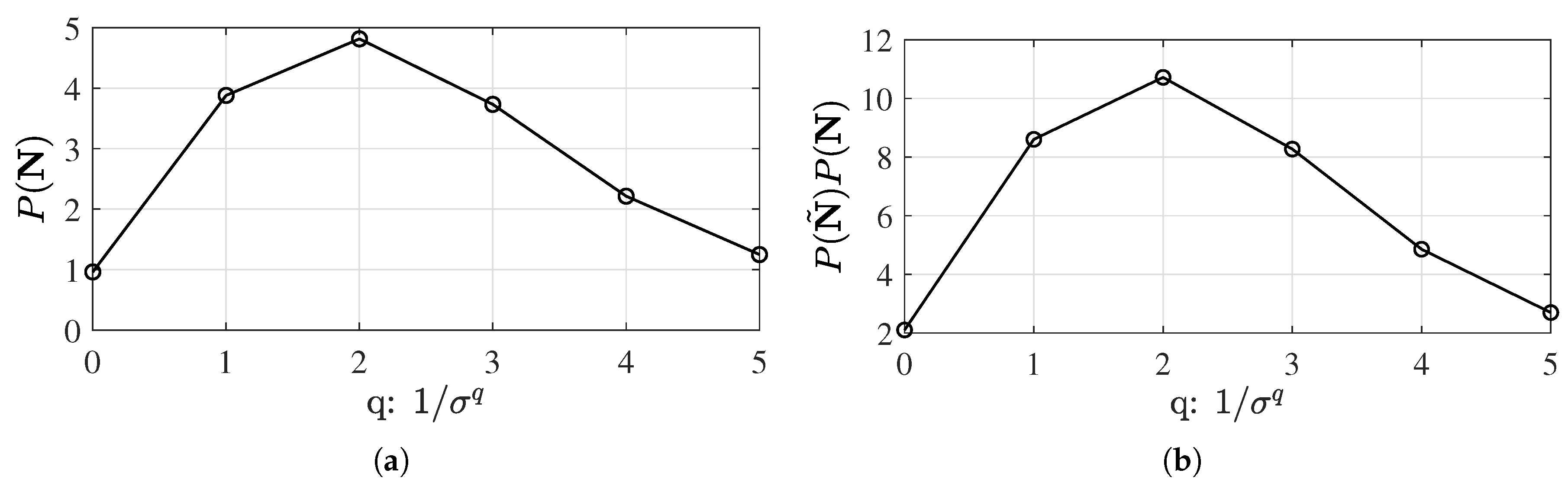
To compare the performance of $1/{\sigma }^q$-type priors, $q=0,\dots 5$ were used to represent the regular least squares, Jeffreys’, and ALI priors. The likelihood of the fitting performance and prediction performance was evaluated using the method of Laplace approximation, and results are shown in Figure 1. The total likelihood of the fitting and prediction results indicates that the Jeffreys’ prior $1/{\sigma }^2$ outperformed the others. The result associated with $q=0$ is the Bayesian version of the regular least squares estimation.

To further demonstrate the difference between the regular least squares and noninformative Bayesian approach under this sample size, the following reliability problem was considered. The fatigue life given a prescribed probability of failure (POF) was calculated for the cyclic strain range ($\Delta \epsilon /2$) between ${10}^{-4}$ and ${10}^{-1}$. Given a cyclic strain range and a POF, the fatigue life $N_{\mathrm{POF}}$ can be expressed as:

$$\mathrm{Pr}(N>N_{\mathrm{POF}})=1-\mathrm{POF}.$$

(40)

For the regular least squares estimator, it can be obtained using the t-statistics given by Equation (A9) where $\gamma /2$ should be replaced with the prescribed POF because only the lower one-sided bound is needed. For the Bayesian with Jeffreys’ prior, the one-side bound can trivially be obtained using the POF-quantile of the prediction results evaluated using MCMC samples of the posterior POF. Figure 2 presents the comparisons of the fatigue life results where the obvious difference was observed. The results of the noninformative Bayesian were larger than those of regular least squares, indicating a longer fatigue life for the same risk level, i.e., ${10}^{-5}$ POF.

4.2. Aeroengine Turbine Disk Lifing and Failure Rate Assessment

The prescribed safe life is a critical parameter for airworthiness and service health management of turbine disks in aeroengines. To determine the prescribed safe life for turbine disks, life testing with a number of disks is performed using disk samples in a rotating pit. The number of tested piece is usually less than five due to the cost and time constraints; sometimes, only one or two test pieces are available. The determination of the prescribed safe life must be carefully made to mitigate the risk. A general and standard procedure described in [41] is centered on the idea that two source of uncertainty, namely the sampling uncertainty and the life distribution uncertainty, should be incorporated. To account for the sampling uncertainty, the 95% single-sided lower bound of the sample mean is used as the mean of the life distribution. To account for the uncertainty of the life distribution itself, no more than one in seven-hundred fifty service disks is allowed to develop an engineering crack. The total safety margin is a 1/750 cumulative failure probability to a 95% confidence.

The prescribed safe life is assumed to be a log-normal random variable, and the log-life is a normally distributed variable. Denote the mean and standard deviation of the normal distribution of the log-life as $ln{N}_{\mathsf{\mu }}$ and $\sigma$. The 95% single-sided lower bound of the sample mean can be expressed as:

$$ln{N}_{\mathsf{\mu }}^{95\%}=ln{N}_{\mathsf{\mu }}-{\lambda }_{\alpha }\frac{\sigma }{\sqrt{n}},$$

(41)

where $N_{\mathsf{\mu }}$ is the geometric mean of the life, $N_{\mathsf{\mu },95\%}$ is the single-sided lower bound of the geometric mean, ${\lambda }_{\alpha }={\Phi }^{-1}(1-\alpha )$, and ${\Phi }^{-1}(·)$ is the inverse cumulative density function (CDF) of the standard normal variable when the standard deviation $\sigma$ is known. For the 95% single-sided lower bound, $z_{\alpha }={\Phi }^{-1}\left(0.95\right)=1.645$. When the standard deviation is unknown, the estimate of the standard deviation based on the samples should be used. In such cases, the value of ${\lambda }_{\alpha }$ is obtained using the Student distribution with a degree of freedom (DOF) of $n-1$, i.e., ${\lambda }_{\alpha }=t^{-1}(1-\alpha ,n-1)$. The function $t^{-1}(·,n-1)$ is the inverse CDF of the Student distribution with a DOF of $n-1$. The 1/750 failure probability log-life corresponds to the $-3\sigma$ shift from the mean of the log-life distribution. When using $ln{N}_{\mathsf{\mu }}^{95\%}$ as the mean of the log-life distribution, the 1/750 failure probability life $N_{\mathsf{\mu }-3\sigma }^{95\%}$ writes:

$$ln{N}_{\mathsf{\mu }-3\sigma }^{95\%}=ln{N}_{\mathsf{\mu }}^{95\%}-3\sigma .$$

(42)

Combine Equations (41) and (42) to have:

$$ln{N}_{\mathsf{\mu }}-ln{N}_{\mathsf{\mu }-3\sigma }^{95\%}={\lambda }_{\alpha }\frac{\sigma }{\sqrt{n}}+3\sigma ,$$

(43)

The safety factor that ensures a 1/750 failure to a 95% confidence can be expressed by transforming Equation (43) into the linear scale as:

$$S=\frac{N_{\mathsf{\mu }}}{N_{\mathsf{\mu }-3\sigma }^{95\%}}=exp\left[\left(\frac{{\lambda }_{\alpha }}{\sqrt{n}}+3\right)\sigma \right]$$

(44)

It is seen that the prescribed safe life depends on the number of tested samples n and the standard deviation of the distribution. The deterministic prescribed safe life $A_r$ is finally obtained as:

$$A_r=N_{\mathsf{\mu }}/S.$$

(45)

The cumulative burst probability when the disk is used y cycles can be expressed as:

$$F_b\left(y\right|x^{\prime })={\int }_0^y\frac{1}{\sqrt{2\pi }{\sigma }_b}exp\left[-\frac{{(t-x^{\prime })}^2}{2{\sigma }_b^2}\right]\mathrm{d}t,$$

(46)

where $x^{\prime }$ is the log-transformed geometric mean of the samples and y is the log-transformed number of cycles, i.e., $y=lnN$. The failure rate in terms of the failures per cycle can be expressed as:

$$h\left(y\right|x^{\prime })=\frac{\partial F_b\left(y\right|x^{\prime })/\partial y}{1-F_b\left(y\right|x^{\prime })}=\frac{f_b\left(y\right|x^{\prime })}{1-F_b\left(y\right|x^{\prime })},$$

(47)

where $f_b\left(y\right|x^{\prime })$ is the burst PDF:

$$f_b\left(y\right|x^{\prime })=\frac{1}{\sqrt{2\pi }{\sigma }_b}exp\left[-\frac{{(y-x^{\prime })}^2}{2{\sigma }_b^2}\right].$$

(48)

The sampling uncertainty in the log-transformed geometric mean $x^{\prime }$ can be quantified using the sampling PDF. The sample mean $x^{\prime }$ distributes according to:

$$f_s\left(x^{\prime }\right)=\left\{\begin{array}{cc}{\displaystyle \frac{1}{\sqrt{2\pi }{\sigma }_s}exp\left[-\frac{{(x^{\prime }-ln{N}_{\mathsf{\mu }})}^2}{2{\sigma }_s^2}\right]}\hfill & \sigma \mathrm{known}\hfill \\ {\displaystyle ln{N}_{\mathsf{\mu }}+\frac{s}{\sqrt{n}}·t(n-1)}\hfill & \sigma \mathrm{unknown}\hfill \end{array}\right.,$$

(49)

where s is the standard deviation of the sample, $t(n-1)$ is the standard Student distribution with a DOF of $n-1$, and ${\sigma }_s=\frac{\sigma }{\sqrt{n}}$.

The final failure rate can be obtained by marginalizing out the sampling error variable $x^{\prime }$ as:

$$h\left(y\right)=\int h\left(y\right|x^{\prime })f_s\left(x^{\prime }\right)\mathrm{d}{x}^{\prime }.$$

(50)

With the above discussion, turbine disk life testing results on two disks were obtained as shown in

Table 3. Spin rig testing results on two disks.

Disk No.	No. of Cycles
1	27,000
2	21,700

.

It is seen that the key information is the standard deviation of the population. For one thing, whether it is considered as a known quantity requires a justification, and its actual value relies on empirical evidence and historical data. For another, when it needs to be estimated from the samples, the proper method should be used due to its limited sample size.

4.2.1. Existing Method

Previous disk life testing results showed that the scatter factor, defined as the ratio of the maximum life ($N_{max}$) over the minimum life ($N_{min}$), is less than six. Furthermore, $N_{max}$ and $N_{min}$ are considered as the $+3\sigma$ and $-3\sigma$ points of the normal distribution of the log-life. With the above empirical evidence and assumption The empirical evidence of $N_{max}/N_{min}=6$, combined with the assumption that $ln{N}_{max}-ln{N}_{min}=6\sigma$, yields:

$$\sigma =\frac{ln{N}_{max}-ln{N}_{min}}{6}=\frac{1}{6}ln\left(\frac{N_{max}}{N_{min}}\right)=\frac{ln6}{6}.$$

(51)

The safety factor that ensures a 1/750 failure to a 95% confidence can be expressed, by substituting Equation (51) into Equation (43) as,

$$S=\frac{N_{\mathsf{\mu }}}{N_{\mathsf{\mu }-3\sigma }^{95\%}}=6^{\frac{1}{2}+\frac{1.645}{6\sqrt{n}}}$$

(52)

Given that assumption that the standard deviation of the log-life distribution is known, the first equation of the right-hand side in Equation (49) is used. In addition, the term $1-F_b\left(y\right|x^{\prime })\approx 1$ for rare events. In such a case, the hazard rate function Equation (50) reduces to the convolution of two normal PDFs, and the resulting hazard rate function is:

$$h\left(y\right)=\int h\left(y\right|x^{\prime })f_s\left(x^{\prime }\right)\mathrm{d}{x}^{\prime }\approx \mathrm{Norm}(y,ln{N}_{\mathsf{\mu }},{\sigma }_b^2+{\sigma }_s^2).$$

(53)

Note that $y=lnN$; the hazard rate in terms of failure per flight hour is found by using the chain rule as,

$$h\left(H\right)=\frac{1}{H}·\mathrm{Norm}(ln\left(\beta H\right),ln{N}_{\mathsf{\mu }},{\sigma }_b^2+{\sigma }_s^2),$$

(54)

where $\beta$ is the exchange rate (cycles/hour) converting the cycle to equivalent engine flight hours. Using the data in Table 3, the log-transformed geometric mean $ln{N}_{\mathsf{\mu }}=$ 24,205, the standard deviation of the log-life distribution is ${\sigma }_b=(ln6)/6$, and the standard deviation of the sampling distribution is ${\sigma }_s=(ln6)/\left(6\sqrt{2}\right)$. Substitute these parameters into Equation (45) to obtain the prescribed safe life as $A_r=6981$ cycles.

4.2.2. The Proposed Noninformative Bayesian Method

Without relying on the empirical evidence and the assumption, the noninformative Bayesian estimator for $(\mathsf{\mu },\sigma )$ of the log-life distribution can be obtained by writing the posterior of the likelihood of samples with a noninformative prior. For a demonstration, the prior of $\propto 1/{\sigma }^2$ was used, and the posterior writes,

$$p(\mathsf{\mu },\sigma |D)\propto \frac{1}{{\sigma }^2}·{\left(\frac{1}{{\sigma }^2}\right)}^{n/2}·exp\left[-\frac{{\sum }_{i=1}^n{(ln{N}_i-\mathsf{\mu })}^2}{2{\sigma }^2}\right],$$

(55)

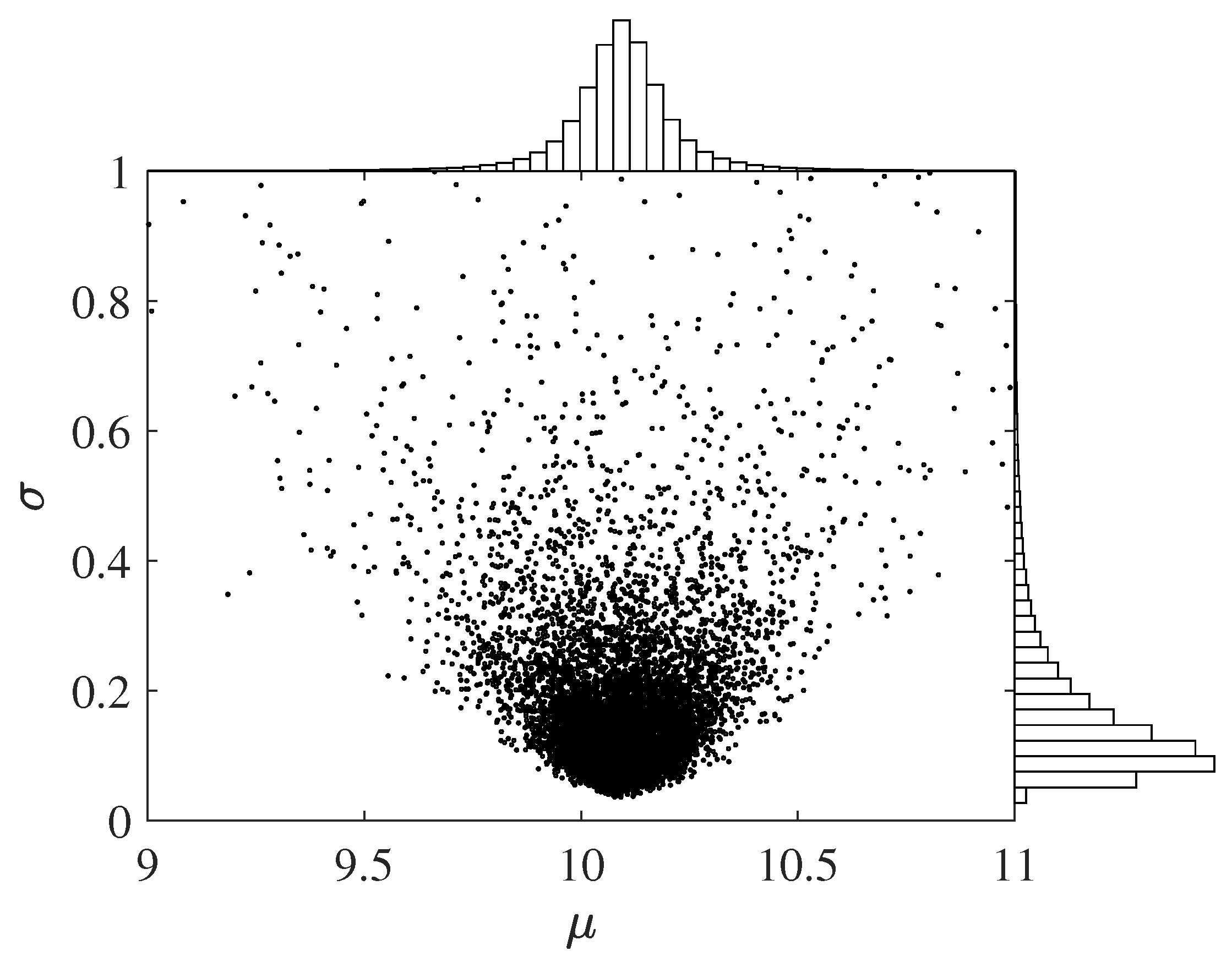
where D denotes the event of observed life samples $N_1,\dots ,N_n$. To estimate $\mathsf{\mu }$ and $\sigma$, $1\times {10}^7$ samples were drawn from Equation (55) using the MCMC method. The resulting histogram of the samples is shown in Figure 3. The 95% single-sided confidence bound ${\mathsf{\mu }}^{95\%}$ can be estimated using the 0.05-quantile of the MCMC samples as $9.86565$ or 19,259 in the linear scale. Centering on ${\mathsf{\mu }}^{95\%}=9.86565$, the value corresponding to a 1/750 cumulative failure probability was found by subtracting ${\mathsf{\mu }}^{95\%}$ by $3\sigma$. The term $\sigma$ was estimated using the MCMC sample mean, and in this case, it was found as $0.1893$. Consequently, after applying the two safety margins, the prescribed safe life (in log scale) using the noninformative Bayesian method was found as ${\mathsf{\mu }}_{-3\sigma }^{95\%}=9.2976$ or $A_r=$ 10,911 cycles.

The failure rates calculated using the existing method and the proposed noninformative Bayesian method are compared in Figure 4. The failure rate per flight hour was based on an exchange rate $\beta =2.5$.

Based on the results shown in Figure 4, the usable flight hours obtained using the noninformative Bayesian method were about 1000 h more than those obtained using the existing method given the same risk constraint. For example, the flight hours corresponding to a failure rate of ${10}^{-8}$/h were 2734 and 1734, respectively, for the two methods. When the failure rate was required to be ${10}^{-6}$/h, the usable flight hours were 3817 and 2720, respectively. It should be noted that the proposed noninformative Bayesian method does not rely on empirical evidence and assumptions other than the log-normal distribution for disk life.

5. Conclusions

The study developed a noninformative Bayesian inference method for small sample problems. In particular, a $1/{\sigma }^q$-type of prior was proposed to formulate the Bayesian posterior. It was shown that this type of prior can represent the classical Jeffreys’ prior (Fisher information), flat prior, and asymptotic locally invariant prior. More importantly, this type of prior was derived as the limiting state of normal-inverse-Gamma (NIG) conjugate priors, allowing for fast and efficient evaluations of the Bayesian posteriors and predictors in closed-form expressions under a Gaussian likelihood. To illustrate the overall method and compare the performance of noninformative priors, a realistic fatigue reliability problem was discussed in detail. The combined fitting and prediction performance in terms of the likelihood was used to evaluate different priors. It was observed that Jeffreys’ prior, $1/{\sigma }^2$, yielded the maximum likelihood. The developed method was further applied to an actual aeroengine disk lifing problem with two test samples, and the results on the prescribed safe life and risk in terms of failure/hour were comparable with those obtained using the existing method incorporating the empirical evidence and assumptions. It should be emphasized that the study did not promote abandoning justified experience and/or information in prior construction. It was argued in this study that in the absence of those data or experience, the noninformative prior should be used to avoid introducing unjustified information into the prior. The following conclusions were drawn based on the current results:

• The $1/{\sigma }^q$-type of prior can be used equivalently as the NIG conjugate priors at their limiting states. The great features of conjugate priors, such as having analytical posterior and prediction PDFs under a Gaussian likelihood, can be retained when using noninformative priors for Bayesian linear regression analysis;
• For the $1/{\sigma }^q$-type of noninformative prior, the classical Jeffreys’ prior $1/{\sigma }^2$ yielded an optimal fitting and prediction performance in terms of the likelihood or Bayes factors. When $q=0$, the Bayesian estimator reduces to the regular least squares estimator. The results of the two case studies showed the advantage of using the noninformative Bayesian estimator with the prior of $\propto 1/{\sigma }^2$ over the regular least squares estimator and other empirical methods under small sample sizes.

References

- Royall, R.M. The effect of sample size on the meaning of significance tests. Am. Stat. 1986, 40, 313–315. [Google Scholar]
- Raudys, S.J.; Jain, A.K. Small sample size effects in statistical pattern recognition: Recommendations for practitioners. IEEE Trans. Pattern Anal. Mach. Intell. 1991, 13, 252–264. [Google Scholar] [CrossRef]
- Nelson, C.R.; Kim, M.J. Predictable stock returns: The role of small sample bias. J. Financ. 1993, 48, 641–661. [Google Scholar] [CrossRef]
- Fan, X.; Thompson, B.; Wang, L. Effects of sample size, estimation methods, and model specification on structural equation modeling fit indexes. Struct. Equ. Model. A Multidiscip. J. 1999, 6, 56–83. [Google Scholar] [CrossRef]
- McNeish, D. On using Bayesian methods to address small sample problems. Struct. Equ. Model. A Multidiscip. J. 2016, 23, 750–773. [Google Scholar] [CrossRef]
- Winkler, R.L. Probabilistic prediction: Some experimental results. J. Am. Stat. Assoc. 1971, 66, 675–685. [Google Scholar] [CrossRef]
- Melchers, R.E.; Beck, A.T. Structural Reliability Analysis and Prediction; John Wiley & Sons: Hoboken, NJ, USA, 2018. [Google Scholar]
- He, J.; Chen, J.; Guan, X. Lifetime distribution selection for complete and censored multi-level testing data and its influence on probability of failure estimates. Struct. Multidiscip. Optim. 2020, 62, 1–17. [Google Scholar] [CrossRef]
- Du, Y.M.; Ma, Y.H.; Wei, Y.F.; Guan, X.; Sun, C. Maximum entropy approach to reliability. Phys. Rev. E 2020, 101, 012106. [Google Scholar] [CrossRef]
- Zhou, D.; He, J.; Du, Y.M.; Sun, C.; Guan, X. Probabilistic information fusion with point, moment and interval data in reliability assessment. Reliab. Eng. Syst. Saf. 2021, 213, 107790. [Google Scholar] [CrossRef]
- Gao, C.; Fang, Z.; Lin, J.; Guan, X.; He, J. Model averaging and probability of detection estimation under hierarchical uncertainties for Lamb wave detection. Mech. Syst. Signal Process. 2022, 165, 108302. [Google Scholar] [CrossRef]
- Gregory, P. Bayesian Logical Data Analysis for the Physical Sciences: A Comparative Approach with Mathematica Support; Cambridge University Press: Cambridge, UK, 2005. [Google Scholar]
- Guan, X.; Jha, R.; Liu, Y. Model selection, updating, and averaging for probabilistic fatigue damage prognosis. Struct. Saf. 2011, 33, 242–249. [Google Scholar] [CrossRef]
- Hamdia, K.M.; Zhuang, X.; He, P.; Rabczuk, T. Fracture toughness of polymeric particle nanocomposites: Evaluation of models performance using Bayesian method. Compos. Sci. Technol. 2016, 126, 122–129. [Google Scholar] [CrossRef]
- Yang, J.; He, J.; Guan, X.; Wang, D.; Chen, H.; Zhang, W.; Liu, Y. A probabilistic crack size quantification method using in-situ Lamb wave test and Bayesian updating. Mech. Syst. Signal Process. 2016, 78, 118–133. [Google Scholar] [CrossRef]
- Wang, D.; He, J.; Guan, X.; Yang, J.; Zhang, W. A model assessment method for predicting structural fatigue life using Lamb waves. Ultrasonics 2018, 84, 319–328. [Google Scholar] [CrossRef]
- Guan, X.; He, J. Life time extension of turbine rotating components under risk constraints: A state-of-the-art review and case study. Int. J. Fatigue 2019, 129, 104799. [Google Scholar] [CrossRef]
- He, J.; Huo, H.; Guan, X.; Yang, J. A Lamb wave quantification model for inclined cracks with experimental validation. Chin. J. Aeronaut. 2021, 34, 601–611. [Google Scholar] [CrossRef]
- Huo, H.; He, J.; Guan, X. A Bayesian fusion method for composite damage identification using Lamb wave. Struct. Health Monit. 2020, 1475921720945000. [Google Scholar] [CrossRef]
- Berger, J.O. Robust Bayesian analysis: Sensitivity to the prior. J. Stat. Plan. Inference 1990, 25, 303–328. [Google Scholar] [CrossRef]
- Berger, J.O.; Moreno, E.; Pericchi, L.R.; Bayarri, M.J.; Bernardo, J.M.; Cano, J.A.; De la Horra, J.; Martín, J.; Ríos-Insúa, D.; Betrò, B.; et al. An overview of robust Bayesian analysis. Test 1994, 3, 5–124. [Google Scholar] [CrossRef]
- Kass, R.E.; Wasserman, L. The selection of prior distributions by formal rules. J. Am. Stat. Assoc. 1996, 91, 1343–1370. [Google Scholar] [CrossRef]
- Bishop, P.; Bloomfield, R.; Littlewood, B.; Povyakalo, A.; Wright, D. Toward a formalism for conservative claims about the dependability of software-based systems. IEEE Trans. Softw. Eng. 2010, 37, 708–717. [Google Scholar] [CrossRef]
- Gelman, A.; Hennig, C. Beyond subjective and objective in statistics. J. R. Stat. Soc. Ser. A 2017, 180, 967–1033. [Google Scholar] [CrossRef] [Green Version]
- Zhang, J.; Shields, M.D. The effect of prior probabilities on quantification and propagation of imprecise probabilities resulting from small datasets. Comput. Methods Appl. Mech. Eng. 2018, 334, 483–506. [Google Scholar] [CrossRef] [Green Version]
- Schervish, M.J.; DeGroot, M.H. Probability and Statistics; Pearson Education: London, UK, 2014. [Google Scholar]
- Jaynes, E.T. Prior probabilities. IEEE Trans. Syst. Sci. Cybern. 1968, 4, 227–241. [Google Scholar] [CrossRef]
- Jaynes, E.; Bretthorst, G. Probability Theory: The Logic of Science; Cambridge University Press: Cambridge, UK, 2003. [Google Scholar]
- Gelman, A.; Simpson, D.; Betancourt, M. The prior can often only be understood in the context of the likelihood. Entropy 2017, 19, 555. [Google Scholar] [CrossRef] [Green Version]
- Jeffreys, H. An Invariant Form for the Prior Probability in Estimation Problems. Proc. R. Soc. Lond. Ser. A 1946, 186, 453–461. [Google Scholar]
- Hartigan, J. Invariant prior distributions. Ann. Math. Stat. 1964, 35, 836–845. [Google Scholar] [CrossRef]
- Bernardo, J.M. Reference posterior distributions for Bayesian inference. J. R. Stat. Soc. Ser. B 1979, 41, 113–147. [Google Scholar] [CrossRef]
- Berger, J.O.; Bernardo, J.M. Ordered group reference priors with application to the multinomial problem. Biometrika 1992, 79, 25–37. [Google Scholar] [CrossRef]
- Jeffreys, H. The Theory of Probability; Oxford University Press: Oxford, UK, 1998. [Google Scholar]
- Gelman, A. Prior distributions for variance parameters in hierarchical models (comment on article by Browne and Draper). Bayesian Anal. 2006, 1, 515–534. [Google Scholar] [CrossRef]
- Simpson, D.; Rue, H.; Riebler, A.; Martins, T.G.; Sørbye, S.H. Penalising model component complexity: A principled, practical approach to constructing priors. Stat. Sci. 2017, 32, 1–28. [Google Scholar] [CrossRef]
- Kullback, S.; Leibler, R. On information and sufficiency. Ann. Math. Stat. 1951, 22, 79–86. [Google Scholar] [CrossRef]
- Guan, X.; He, J.; Jha, R.; Liu, Y. An efficient analytical Bayesian method for reliability and system response updating based on Laplace and inverse first-order reliability computations. Reliab. Eng. Syst. Saf. 2012, 97, 1–13. [Google Scholar] [CrossRef]
- He, J.; Guan, X.; Jha, R. Improve the accuracy of asymptotic approximation in reliability problems involving multimodal distributions. IEEE Trans. Reliab. 2016, 65, 1724–1736. [Google Scholar] [CrossRef]
- American Society for Testing and Materials. ASTM E739-10(2015)-Standard Practice for Statistical Analysis of Linear or Linearized Stress-Life (S-N) and Strain-Life (ε-N) Fatigue Data; ASTM International: West Conshohocken, PA, USA, 2015. [Google Scholar]
- Boyd-Lee, A.; Harrison, G.; Henderson, M. Evaluation of standard life assessment procedures and life extension methodologies for fracture-critical components. Int. J. Fatigue 2001, 23, 11–19. [Google Scholar] [CrossRef]
- Browne, W.J.; Draper, D. A comparison of Bayesian and likelihood-based methods for fitting multilevel models. Bayesian Anal. 2006, 1, 473–514. [Google Scholar] [CrossRef]
- Kotz, S.; Nadarajah, S. Multivariate T-Distributions and Their Applications; Cambridge University Press: Cambridge, UK, 2004. [Google Scholar]
- Graybill, F.A.; Bowden, D.C. Linear segment confidence bands for simple linear models. J. Am. Stat. Assoc. 1967, 62, 403–408. [Google Scholar] [CrossRef]
Figure 1.
(a) MCMC samples drawn from the noninformative Bayesian posterior with Jeffreys’ prior () and (b) the fatigue life results at obtained with the regular least squares (LS) estimator and noninformative Bayesian (NB).
Figure 2.
(a) The fitting performance evaluated with different priors and (b) the prediction performance evaluated with different priors. One data point is considered for the prediction.
Figure 3.
Samples drawn from the posterior PDF and histograms.
Figure 4.
Comparisons of the failure rate results of the two methods. The solid line and the dashed line are results from the noninformative Bayesian (NB) and existing method (Ref.), respectively.