Real-World Data-Driven Machine-Learning-Based Optimal Sensor Selection Approach for Equipment Fault Detection in a Thermal Power Plant

Abstract

Due to growing electricity demand, developing an efficient fault-detection system in thermal power plants (TPPs) has become a demanding issue. The most probable reason for failure in TPPs is equipment (boiler and turbine) fault. Advance detection of equipment fault can help secure maintenance shutdowns and enhance the capacity utilization rates of the equipment. Recently, an intelligent fault diagnosis based on multivariate algorithms has been introduced in TPPs. In TPPs, a huge number of sensors are used for process maintenance. However, not all of these sensors are sensitive to fault detection. The previous studies just relied on the experts’ provided data for equipment fault detection in TPPs. However, the performance of multivariate algorithms for fault detection is heavily dependent on the number of input sensors. The redundant and irrelevant sensors may reduce the performance of these algorithms, thus creating a need to determine the optimal sensor arrangement for efficient fault detection in TPPs. Therefore, this study proposes a novel machine-learning-based optimal sensor selection approach to analyze the boiler and turbine faults. Finally, real-world power plant equipment fault scenarios (boiler water wall tube leakage and turbine electric motor failure) are employed to verify the performance of the proposed model. The computational results indicate that the proposed approach enhanced the computational efficiency of machine-learning models by reducing the number of sensors up to 44% in the water wall tube leakage case scenario and 55% in the turbine motor fault case scenario. Further, the machine-learning performance is improved up to 97.6% and 92.6% in the water wall tube leakage and turbine motor fault case scenarios, respectively.

1. Introduction

Modern thermal power plants are highly complex and are equipped with advanced data acquisition systems [1]. A huge amount of sensor data is generated and stored in the historical database of TPPs. These historical data represent the health state of the power plant that can be used for performance monitoring, fault detection, and isolation. The early detection and diagnosis of the faults in a thermal power plant can help implement shorter shutdowns, reduced maintenance, and lower generation costs [2].

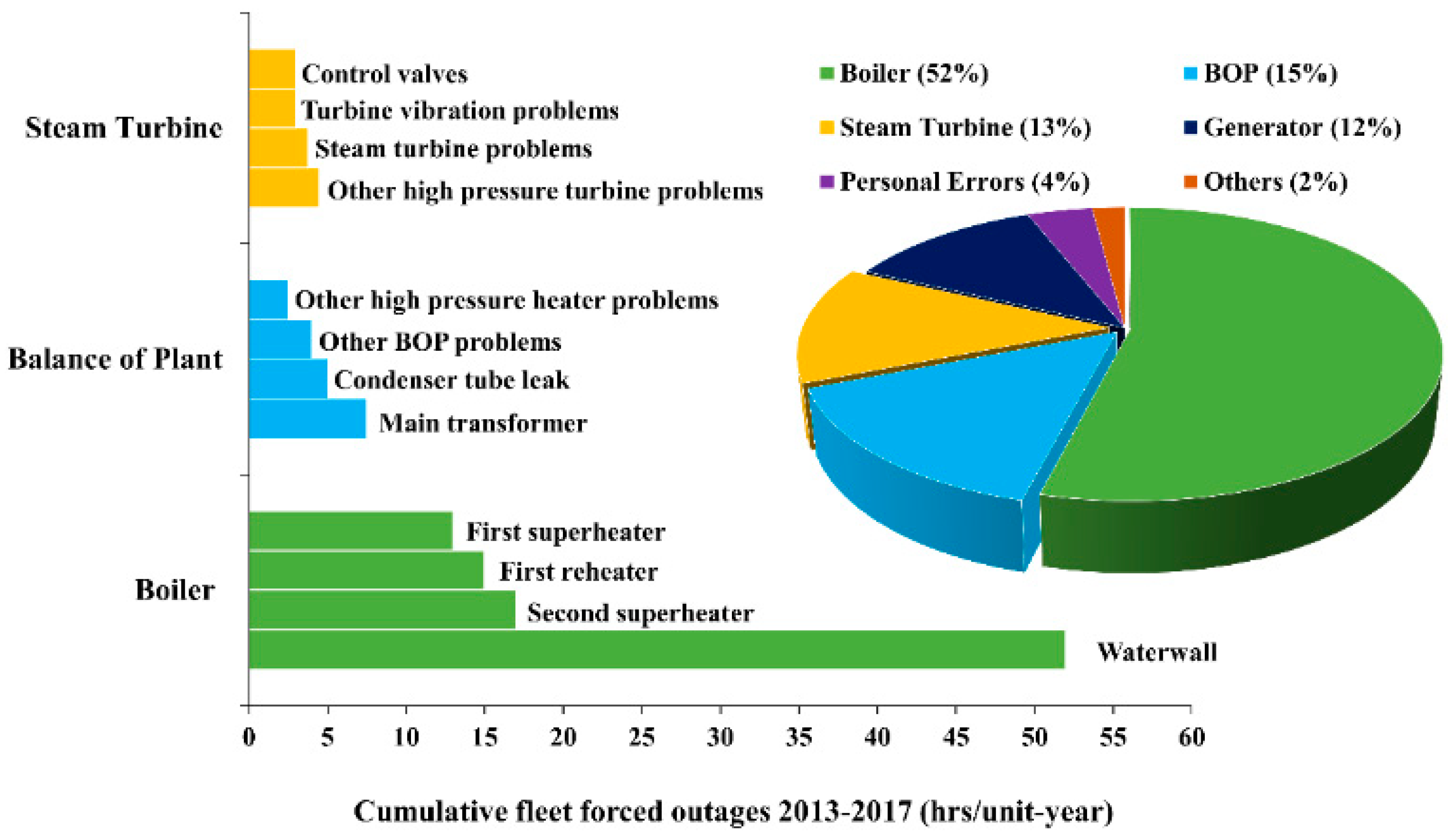
Boiler tube leakage is the most probable failure in a thermal power plant. Approximately 60% of boiler shutdowns are caused by boiler tube leakages [3]. The most dominant occurrence of leakage occurs in the water wall tube section [4]. The tube leakage arises due to corrosion [5], erosion [5], and fatigue [6], which cause the tube wall thickness to decrease, leading to tube rupture and failure. Recently, an e-maintenance-based system [7] utilizing the process monitoring data was introduced for an intelligent fault diagnosis in TPPS. The process control data can provide sufficient information for effective tube leakage detection [8]. Jungwon et al. [9] utilized the thermocouples sensors data mounted on the final superheater outlet header of an 870 MW coal-fired power plant and proposed a principal component analysis (PCA)-based tube leakage detection approach. The proposed method could successfully detect tube leakage. Recently, Natarianto et al. [10] used process control data and introduced a data analytics-based approach by combining PCA, canonical variate, and linear discriminant analysis (LDA) for water wall tube leakage detection in a 650 MW supercritical coal-fired thermal power plant. Swiercz et al. [11] proposed a multiway PCA approach for boiler riser and downcomer tube leakage detection using expert-provided sensor data. The proposed method could successfully detect the tube leak 3–5 days before boiler shutdown.

Steam turbines are another vital piece of equipment used as the primary energy-generating source in a thermal power plant [12]. Steam turbines consist of multistage steam expansion that makes them complex dynamic structures. The most common faults occurring in the steam turbine are unbalancing, gear fault, looseness, and bearing fault [13]. These faults can stop the smooth operation of the steam turbine and jeopardize reliable power generation. Various research in the past decade has investigated efficient fault detection in steam turbines using historical process data or expert knowledge about the system. The anomalies in the process data can be recognized for each type of failure. Different failures can be further classified using supervised learning. Karim et al. [14] proposed a fault detection and diagnosis approach in an industrial 440 MW steam turbine using four sensitive monitoring parameters. Under challenging noise measurements, twelve major faults were successfully classified using adaptive neuro-fuzzy inference (ANFIS) classifiers. Arian et al. [15] used process monitoring data generated from an Indonesian government steam power plant and proposed a data-driven approach for fault detection in a steam turbine using a neural-network-based classifier.

Generally, a huge amount of sensors are used in power plants for process maintenance [16]. However, not all of these sensors are sensitive to fault detection. The studies mentioned above only depend on expert experience in selecting sensitive sensors to detect boiler and turbine faults. However, redundant and irrelevant sensors may influence multivariate algorithms that are highly reliant on the number of input sensors. Thus, an accurate methodology is needed to select the relevant sensors necessary to detect boiler and turbine failures. Recently, machine-learning algorithms have gained importance for intelligent fault detection and diagnosis in thermal power plants [17]. These machine-learning algorithms are typically combined with dimensionality reduction methods, such as PCA, to eliminate unnecessary data [18,19]. However, these approaches do not help identify the cause of failure, nor do they distinguish the most relevant sensors. The feature selection approaches can overcome the challenges mentioned above by simultaneously identifying the relevant sensors and removing different feature selection techniques that are available in the literature, which can be categorized into three categories: optimization-based feature selection [20], regression-based feature selection [21], and classification-based feature selection [22]. For a TPP application, the optimal sensor selection algorithm should have lower complexity and computational cost. 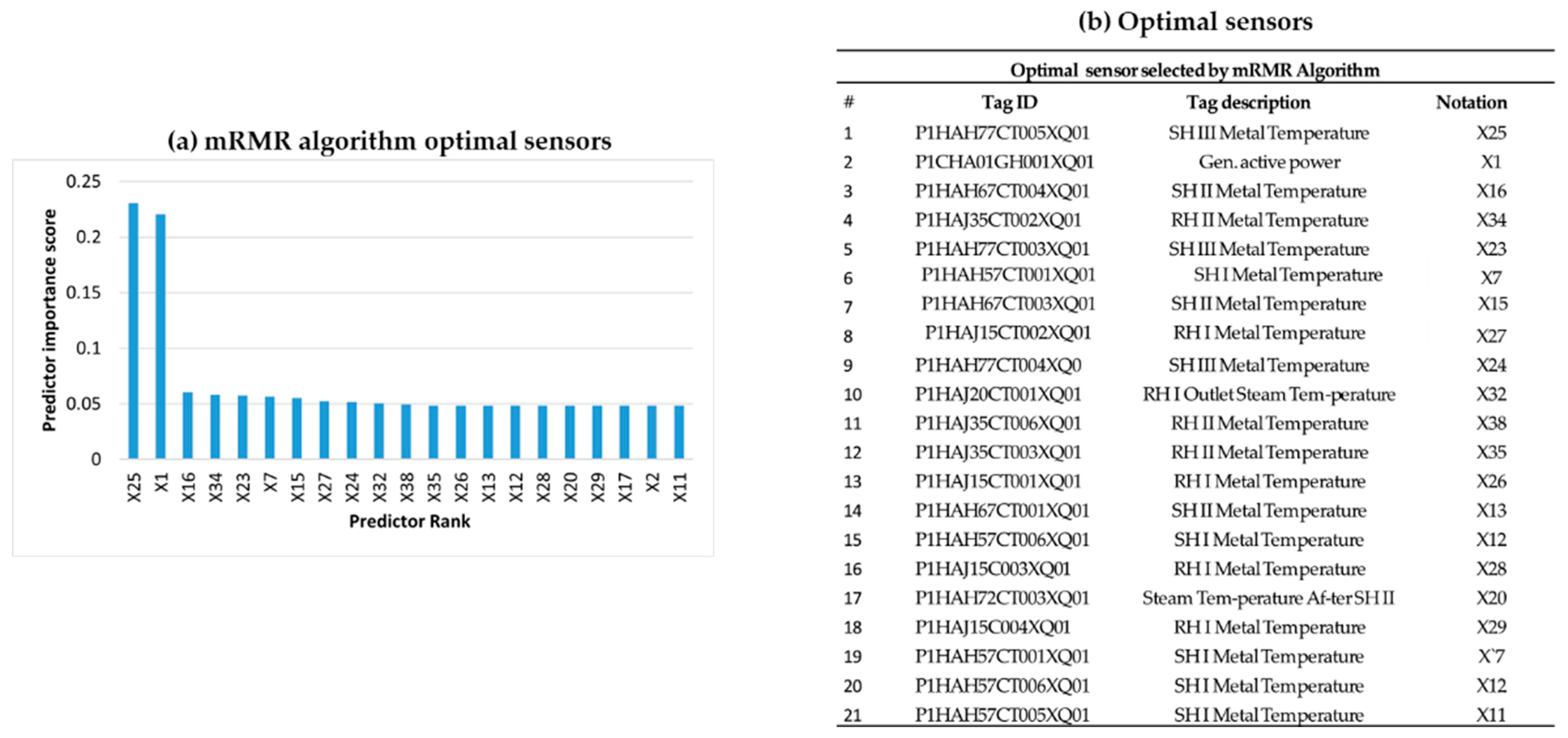For that purpose, correlation analysis is a well-known approach that estimates the relationship between the pairwise input by using the correlation function and removing the redundant and irrelevant features [23]. 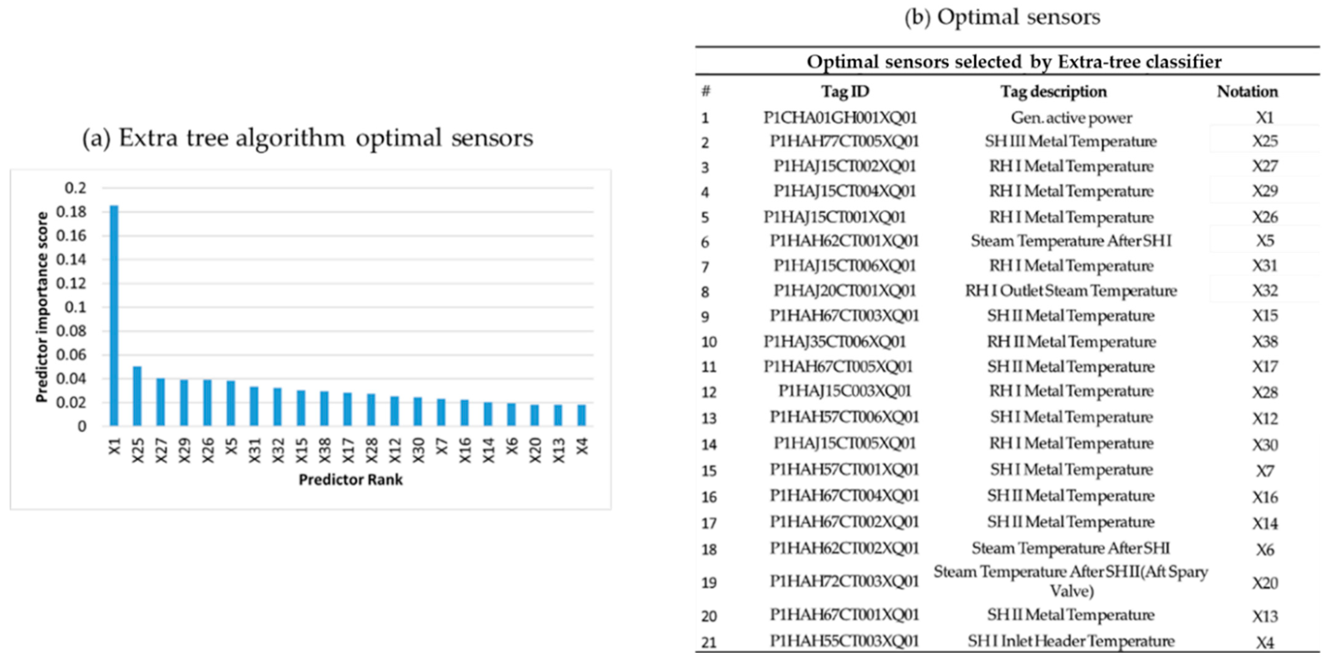Recently, the maximum relevance minimum redundancy (mRMR) algorithm [24] has gained importance, due to its simultaneous ability to minimize redundancy while controlling relevancy among the features. Extra tree classifier [25] is another feature selection technique that has gained popularity among researchers because of its explicit meaning, simple properties, and easy conversion to “if–then rules”. This technique is helpful in problems involving a vast number of numerical features. Therefore, this study utilizes the above-mentioned three approaches for the optimal sensor arrangement in TPPs.

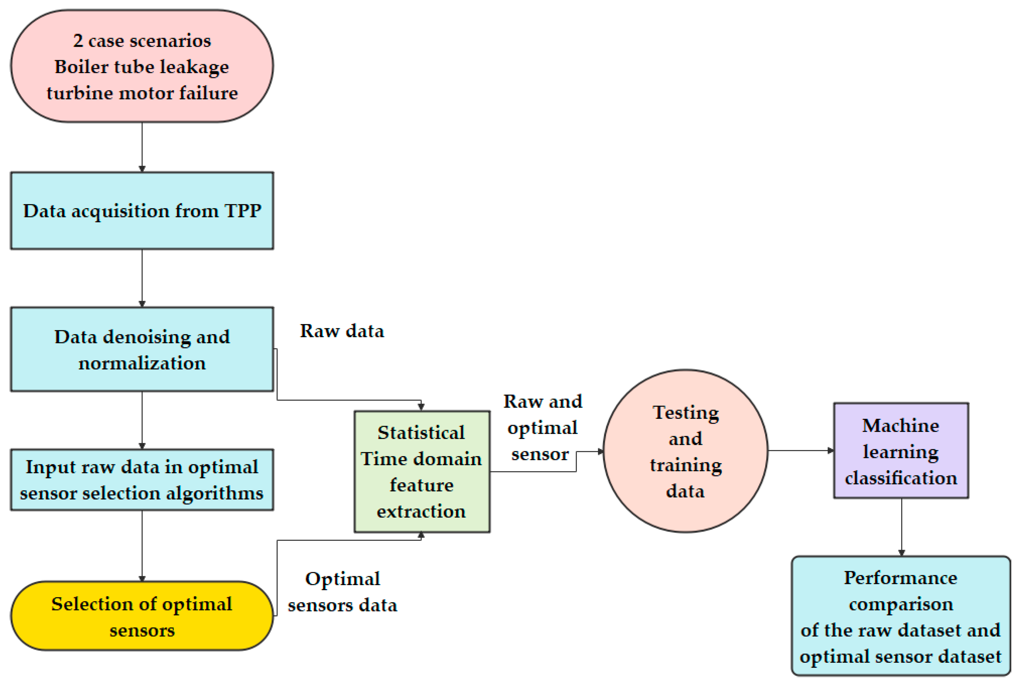
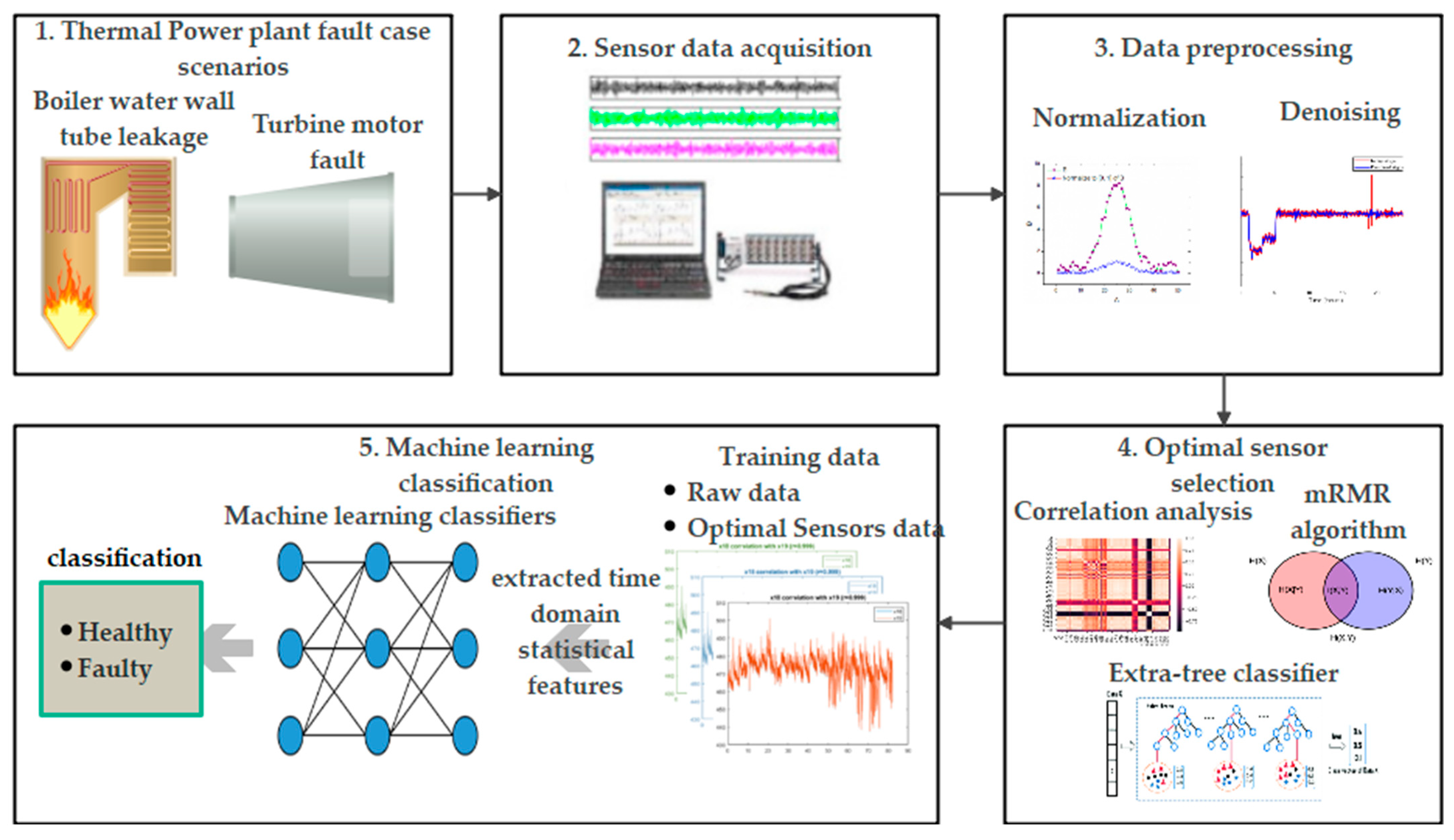
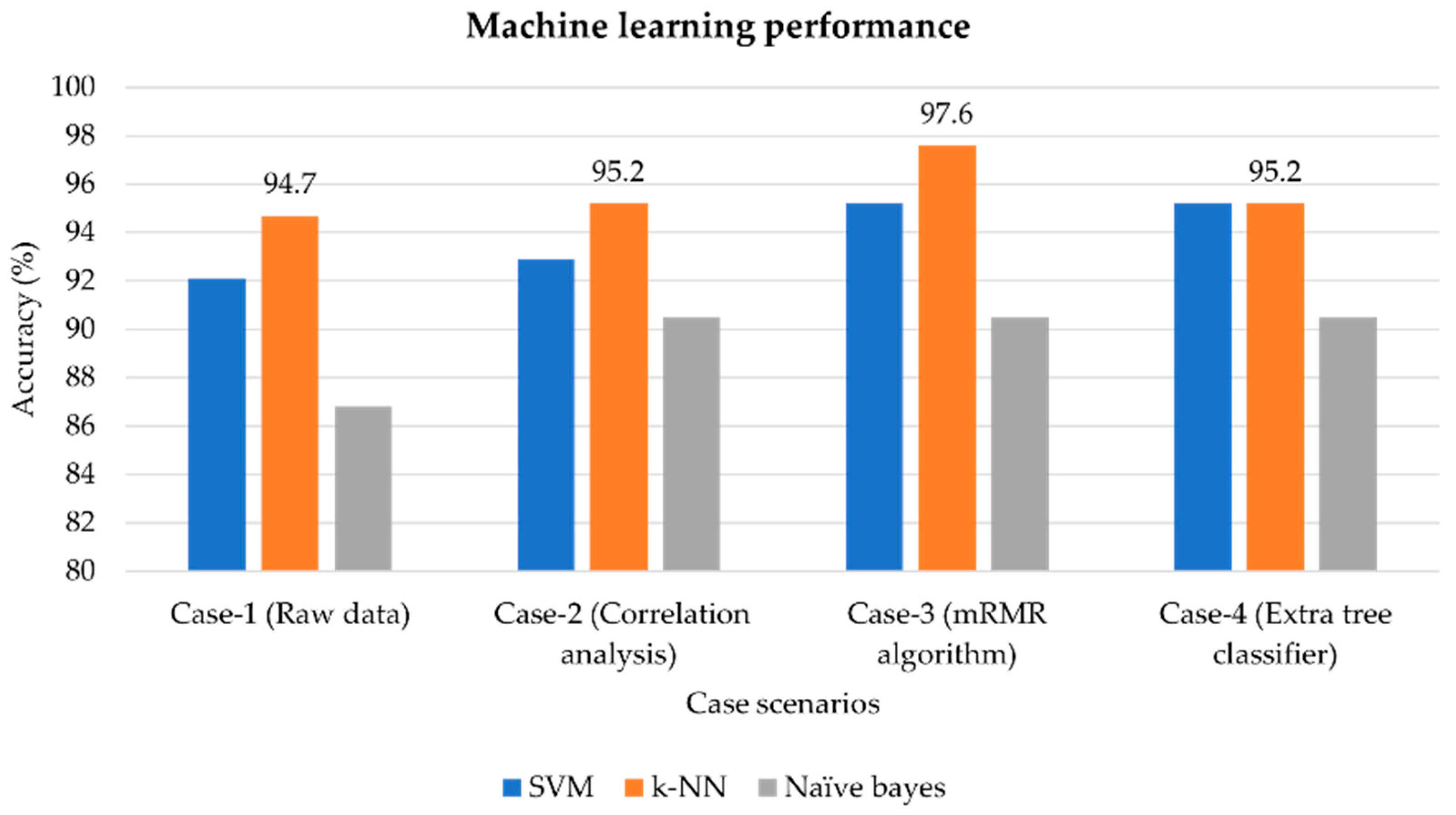
This paper proposes a data-driven machine-learning-based optimal sensor selection approach for thermal power plant boiler and turbine faults. The study performs optimal sensor selection via different feature selection techniques (correlation, mRMR, and extra-tree classifier). Three supervised machine-learning classifiers (support vector machines, k-nearest neighbor, and naïve Bayes) are used for the fault classification. In the end, two real-world power plant equipment fault scenarios (boiler water wall tube leakage and turbine electric motor failure) are employed to verify the performance of the proposed model.

State-of-the-Art Literature Survey

This section lists the state of the art techniques used for equipment (boiler and turbine) fault detection in TPPs. Due to the significant importance of the boiler and turbine in TPPs, numerous attempts have been made to detect the equipment fault detection in TPP by using three main approaches, namely, the model-based method [26], the knowledge-based method [27], and the statistical analysis method [28]. A model-based approach is a conventional approach that uses static and dynamic models of the processes. In most cases, it can provide an efficient solution for fault detection. However, it cannot give correct fault detection results because it is difficult to obtain a correct mathematical model due to the complex operations of industrial systems. For a complex system with unknown models, a knowledge-based approach can be used to detect faults. This approach utilizes the rich industrial operational experience of the operators and includes the expert system method. However, this approach cannot identify the most sensitive process variables (sensors) needed to detect the faults in TPPs. Recently, statistical techniques based on multivariate algorithms such as PCA and ANNS are being used to monitor the processes with a large number of variables, such as in TPPs. However, the performance of these multivariate algorithms is highly dependent on the number of input process variables. Therefore, this study proposes an optimal sensor selection approach to identify the most sensitive sensors needed to detect equipment faults in TPPs.

Table 1. State-of-the-art literature survey boiler and turbine fault detection in TPP.

Approach	Application	Year	Contribution	Limitation
Model-based approach	Boiler tube leakage detection [26]	1997	Developed the least-square method with forgetting factor derivation for leak detection	- Challenging to obtain a valid process mathematical model
	Boiler tube leakage detection [29]	2008	Developed the input/output loss method by computing fuel chemistry, heating value, and fuel flow
	Turbine fault detection [30]	2012	Used the time-delay multilayer perceptron model for residual generation for fault detection in industrial turbine
	Turbine fault detection [31]	2011	A nonlinear dynamic model with a dynamic tracking filter was used to detect turbine fault
Knowledge-based approach	Boiler tube leakage detection [27]	1998	Used radiation heat flux measurements for boiler tube leak detection	- Experts provided sensors data - Unknown important monitoring process variables (sensors)
	Boiler tube leakage detection [32]	2016	Developed artificial neural network (ANN) models to detect tube leak
	Turbine fault detection [13]	2017	Developed artificial neural network (ANN) models to detect a fault in steam turbine
Statistical analysis approach	Boiler tube leakage detection [11]	2020	Used multiway PCA model to detect boiler tube leakage	- Performance highly dependent on the number of input sensor variables - Need to find optimal sensors necessary for fault detection
	Boiler tube leakage detection [9]	2017	Applied PCA to tube temperature data to detect boiler tube leakage
	Turbine fault detection [15]	2011	A generalized discriminant analysis approach is used for steam turbine fault detection
	Turbine fault detection [23]	2011	Proposed a support vector machine (SVM)-based model for fault detection in steam turbine

covers the state of the art literature survey for the three main approaches (model-based, knowledge-based, and statistical analysis) used for boiler and turbine fault detection in TPP.

2. Overview of a Coal-Fired Thermal Power Plant

The current study is conducted for a coal-fired TPP. This section gives a brief introduction of a TPP and covers the significance of the boiler and the steam turbine in a TPP.

The modern thermal power plants are developed to a great extent, but the essential equipment in a TPP is more or less the same, with a lot of sophistication and advancement to increase efficiencies [33]. Figure 1 shows the essential equipment in a coal-fired TPP. Steam is generated in the boiler and provided to the steam turbine. The steam turbine expands the steam and rotates the generator to supply electricity. The condenser condenses the turbine steam by transferring the heat to the cooling water supplied from the cooling tower.

2.1. Boiler Water Wall Tube Leakage and Its Significance in a Thermal Power Plant

Bursting of the boiler water wall tube is a severe threat to the continuous and smooth operation of a TPP. In a recent survey conducted by Kokkinos et al. [34], water wall tube leakage is the dominant failure mode in the different TPPs, followed by the final superheater (SH III), first reheater (RH I), and the first superheater (SHI), as Figure 2 shows. Boiler tube leaks represent 52% of the total outages in a TPP.

A TPP shutdowns, whether planned or unplanned, can cause significant financial losses among which boiler tube leakage is the most dominant failure to cause power plant shutdowns. An extensive repairing cost ranging from 2 to 10 million dollars is typically required to repair these leaks [29]. Yong et al. [35] utilized the decision-tree-based method to carry out the cost analysis of the economizer tube leaks in TPP. Considering the electricity market price of 25 dollars/MWh, the expected repair prices are shown for different repair time intervals (repair immediately, delay two days, delay four days, and delay six days). By delaying the repair, the amount of expected repair cost increased significantly.

The water wall tubes are located close to the furnace, and due to the presence of high operating temperature, flue ash erosion, and creep, tube leakage occurs. Liu et al. [36] found that the water wall tube bursts because of overheating under high operating pressure. Yang et al. [37] investigated the coal quality and found that the coal used in TPPs has high ash content that causes corrosion in water wall tubes. It was concluded that suitable coal blending could reduce the corrosion in water wall tubes. Similarly, Xue [38] et al. analyzed the boiler water and found that the presence of NaOH causes corrosion-induced perforation leakage in water wall tubes. To prevent water wall tube leakage, power plant inspectors should inspect water quality to avoid tube leakage, and water quality testing should be performed regularly.

2.2. Turbine Motor Failure Analysis

The reliability of the steam turbine is highly dependent on the reliable functioning of its hydraulic lubrication and control oil system [39]. An essential requirement is a reliable oil supply over the whole operating range. The oil pumps used for that purpose provide the lube oil [40]. The oil pumps are directly driven by an electric motor (AC supply). In the absence of oil supply, bearing failure of the rotating machinery in the steam turbine can occur. This usually happens when an electric pump-driven motor fails due to a power failure or malfunction of the protection system. Therefore, the reliability of the main oil pump depends to a large extent on the AC electric motor. Different studies have been carried out to analyze the AC electric motors [41]. It was found that 40 percent of the failures of AC motor occur due to the failure of the rolling bearing [42]. Therefore, it is recommended to diagnose the bearing condition on time, before failure occurs [43]. The other most prevalent faults in AC motors are winding, unbalanced stator and rotor, broken rotor bar, and eccentricity [44].

Recently, data-driven condition-based monitoring has gained importance in TPPs for efficient fault detection and diagnosis [45]. There are two main steps involved in condition-based monitoring. The first step consists of the data acquisition phase, which represents the health state of the object. For process control and monitoring, there are many sensors employed on the different components in the power plant. This sensor data can provide healthy and faulty state patterns that can be distinguished and classified using multivariate algorithms. In the second step, data preprocessing is carried out that involves multivariate algorithms to classify the preprocessed data. Thus, water wall tube leakage and turbine motor fault detection can be considered classification problems.

3. The Proposed Methodology

This section covers the proposed optimal sensor selection methodology and fault detection by using supervised machine-learning algorithms. The study is divided into three phases. In the first phase, the sensors that are essential for fault detection are distinguished by TPP experts. Those sensors are acquired and preprocessed for the optimal sensor selection process. The second phase utilizes the optimal sensor selection techniques to determine the most sensitive sensors. In the last phase, machine-learning algorithms are employed to detect the equipment (boiler and turbine) faults in TPPs and evaluate the performance of the sensor selection algorithms. The schematic of the proposed methodology is shown in Figure 3.

3.1. Data Acquisition and Preprocessing

In a TPP, it is difficult to learn the exact moment of a fault occurrence, such as a tube leakage location, and the severity of the tube leakage. Therefore, the fault detection algorithm must estimate the appropriate sensors for fault detection. Power plant historical process control data consist of thousands of process variables (sensors). However, none of those sensors are sensitive to specific faults. Therefore, the essential monitoring parameters should be carefully chosen for efficient fault detection. Power plant experts with years of experience usually carry out this process.

Power plant data tend to be inconsistent and noisy; therefore, data preprocessing is required [46]. In the literature, different noise removal techniques are being used. The traditional methods include Fourier transform analysis [47] and power spectral density analysis [48]. However, these techniques are more sensitive towards hidden oscillation and cannot obtain hidden frequencies. On the other hand, wavelet denoising has recently gained popularity in data denoising, because of its capability to simultaneously analyze both the time and frequency domains [49,50]. The wavelet works by decomposing the signal in the time and frequency domains. The selection of an optimal threshold is required to optimize the noise removal. Equation (1) shows the wavelet transform of the continuous signal:

$$\mathrm{WT}.\left(a,b\right)=\underset{-\infty }{\overset{\infty }{{\displaystyle \int }}}\mathrm{x}\left(\mathrm{t}\right)\overline{\psi }\left(\frac{\mathrm{t}-b}{a}\right)\mathrm{dt}$$

(1)

where ψ(t) is the analyzing wavelet, a is the scale parameter, and b is the position parameter.

3.2. Optimal Sensor Selection

In a TPP, piping and instrumentation (P&ID) diagrams monitor all the sensors and equipment. Figure 4 shows the P&ID diagram of the low-pressure (LP) turbine section. There are six thermocouple sensors with unique sensor IDs attached on the furnace wall at separate locations. Similarly, in the P&ID diagram of the LP turbine, six thermocouple sensors are connected to the LP turbine casing. These localized attached sensors may contain redundant knowledge, thus influencing the performance of the multivariate algorithms. Therefore, it is important to downsize the input sensors and determine the appropriate sensor arrangement for equipment fault detection in a TPP.

This study used three different optimal sensor selection approaches (correlation analysis, mRMR algorithm, and extra-tree classifier). The details of the approaches are as follows.

3.2.1. Correlation Analysis

Correlation analysis is a well-known technique and is usually preferred because of its ease of implementation, lesser complexity, and lower computational cost [51]. This analysis evaluates the strength and relationship between the two sensors [52]. Pearson’s coefficient values range (−1 to 1). The value of 1 represents a high positive correlation, while −1 represents a negative correlation between the two sensors. Equation (2) shows how Pearson’s correlation (r) coefficient is calculated:

$$r=\frac{s\left({{\displaystyle \sum }}^{ }ab\right)-\left(a\right)\left({{\displaystyle \sum }}^{ }b\right)}{\sqrt{\sqrt{\left[\left[s{{\displaystyle \sum }}^{ }{b}^2-{\left({{\displaystyle \sum }}^{ }b\right)}^2\right]\right]\left[s{{\displaystyle \sum }}^{ }{a}^2-{\left({{\displaystyle \sum }}^{ }a\right)}^2\right]}}}$$

(2)

where $s$ is the sensor data size, and $a$ and $b$ are the two input sensor variables.

The sensors with high correlation represent the same data trend, and removing the highly correlated sensor may not influence the functioning of the multivariate algorithms. Therefore, in this study, highly correlated sensors are discarded, while keeping one of the highly correlated sensors. The step-by-step implementation of the correlation analysis for the selection of optimal sensors is shown below:

1st step: Calculation of Pearson’s correlation coefficient between all the sensor signals by using Equation (2).

2nd step: Construction of the correlation matrix representing the correlation between all the sensors.

3rd step: The sensors with a correlation value equal to or greater than 0.95 are considered highly correlated.

4th step: Highly correlated sensors are discarded while keeping one of the highly correlated sensors.

3.2.2. mRMR Algorithm

mRMR is an approach recently proposed by Peng et al. [53] and has gained considerable importance in mechanical fault diagnosis and structural health monitoring. mRMR selects the best features in the workspace by minimizing redundancy and maximizing relevancy. It exhibits fast calculation and strong robustness qualities [54]. Hence, our study adopted this method to find the optimal sensors needed for effective fault detection in a TPP. The theoretical background of the mRMR algorithm is summarized as follows.

The algorithm first calculates the mutual information between the attributes X and Y to quantify the relevance and redundancy. Mutual information is defined as follows:

$$I\left(X,Y\right)={{\displaystyle \iint }}^{ }p\left(x,y\right)log\frac{p\left(x,y\right)}{p\left(x\right)p\left(y\right)}$$

(3)

where p(x,y) is the joint probabilistic density, and p(x) and p(y) are marginal probabilistic densities.

Let $S$ denote the sensor dataset, while $S_s$ represents the already selected sensor dataset that contains $m$ sensors, and $S_t$ denotes the to-be-selected sensors, with the dataset consisting of $n$ sensors. The relevance $D$ of the sensor $f$ in$S_t$with the target $c$ can be calculated as:

$$D=I\left(f,c\right)$$

(4)

The redundancy $R$ of the sensor $f$in $S_t$ with all the sensors in $S_s$ can be calculated as:

$$R=\frac{1}{m}{\displaystyle \sum }_{fi\in S_s}I\left(f,c\right)$$

(5)

To obtain the sensor $f_j$ in $S_t$ with maximum relevancy and minimum redundancy, Equations (5) and (6) are combined with the mRMR function:

$${}_{f_j\in S_s}{}^{max}\left[I\left(f_j, c\right)-\frac{1}{m}{\displaystyle \sum }_{f_i \in S_s}I\left(f_j,f_i\right)\right]\left(j=1,2\dots n\right)$$

(6)

For the sensor dataset with $N\left(=m+n\right)$ sensors, the sensor evaluation will continue N rounds. After these evaluations, the optimal sensor set $O$ by mRMR is obtained:

$$O=\left\{f_1^{\prime },f_2^{\prime }\dots .,f_h^{\prime }\dots ,f_n^{\prime }\right\}$$

(7)

The sensor index $h$ represents the importance of the sensor. The more important the sensor, the smaller its index $h$.

The overall steps involved in the computation of optimal sensor selection by using the mRMR algorithm is described below:

1st step: Mutual information is computed between the sensors by using Equation (3).

2nd step: The relevancy and redundancy of the sensor are computed by Equations (4) and (5).

3rd step: Equation (6) is used to obtain the sensor with maximum relevancy and minimum redundancy.

4th step: Score is computed for each sensor to be evaluated, and the sensors with a high score are chosen as optimal sensors.

3.2.3. Extra-Tree Classifier (ETC)

The extra-tree classifier is an ensemble learning technique that accumulates the results of multiple decorrelated decision trees. Each decision tree selects the optimal feature by splitting the data based on the entropy value. The entropy of the feature estimates the quality of the split, as shown in Equation (8). The features belonging to the same class have zero entropy value. Thus, the extra-tree classifier works by recursively selecting node splits with the lowest entropy value:

$$Entropy \left(E\right)=-{\displaystyle \sum }_{i=1}^c{p}_{i}lo{g}_2\left(p_i\right)$$

(8)

where $c$ is the number of class labels, and $p_i$ is the portion of the samples that belong to class $i$.

This study uses the extra-tree classifier because of its simple properties, easy conversion to “if–then” rules, and randomizing property for numerical input [25]. Such advantages make an extra-tree classifier useful for many input sensors and, in such situations, may increase accuracy. The step-by-step implementation of the extra-tree classifier is described as follows:

1st step: Computation of the entropy of the data by using Equation (8).

2nd step: Calculation of the total score for each sensor.

3rd step: Selection of the sensors with a high predictor importance score.

3.3. Machine-Learning Classifiers

Recently, supervised machine learning has gained importance in intelligent fault detection and condition monitoring [55]. Due to labeled data, the results generated from supervised machine learning are more accurate than that from other machine-learning types, such as unsupervised machine learning and reinforcement learning. In this study, three well-known supervised machine-learning classifiers (support-vector machine (SVM), k-nearest neighbors (k-NN), and the naïve Bayes algorithm (NB)) are used for the fault classification.

Due to its tendency to avoid overfitting and its ability to solve complex problems, SVM is commonly used for fault detection applications [56]. SVM forms the hyperplane between the two classes and adjusts the boundary by expanding the distance between the two classes [57]. SVM uses the kernel functions [58] for the nonlinear and inseparable dataset cases. This study utilizes the RBF kernel function due to its higher robustness and infinite smoothness. k-NN is the second supervised machine-learning algorithm used in this study, which classifies the target by calculating its distance from the nearest feature space. k-NN is chosen in this study because of its ease of execution and requires no new parameters to tune. The third algorithm used in this study is naïve Bayes, which is based on the Bayesian theorem [59], and is commonly used for large datasets. Naïve Bayes is chosen in this study because of its higher classification speed and ease of implementation.

Before executing the machine-learning model in real-world applications, its performance must be estimated to verify its extrapolation ability and generalization. Different validation techniques are available in the literature, among which k-fold cross-validation is the most popular [60]. In this study, fivefold cross-validation is used to evaluate the training accuracies of the machine-learning models used.

4. Real-World Power Plant Scenarios—Computational Results

In this section, two real power plant fault case scenarios (boiler water wall tube leakage and turbine motor fault) are employed to validate the performance of the proposed approach. The fault case scenarios analyzed in this study are shown in

Table 2. Description of fault case scenarios.

#	Fault Type	Fault Classification
1	TPP boiler water wall tube leakage	- Healthy state - Leakage state
2	TPP turbine motor failure	- Healthy state - Faulty state

.

The data obtained from the TPP consist of the time domain signals of the expert’s selected process variables (sensors). The detailed description of the acquired data is shown in Figure A1 and Figure A2. The process variables are stored in the historical database of a TPP with a sampling period of 1 s. Ten days of data at the normal working condition of the power plant and 10 days of data from the fault state were acquired from the TPP. As this study focused on the early-stage fault detection of TPP, the data should be provided according to the different fault severity levels so that the fault could be detected at the low severity level of the fault stage. However, the data were not acquired in controlled lab conditions. Therefore, it was not possible to create faults with different severity levels and obtain the data accordingly. This is the main limitation of the acquired data from TPP. Figure 5 shows a schematic of the proposed model for TPP boiler water wall tube leakage detection.

4.1. Case Scenario 1—Boiler Water Wall Tube Leakage

This section implements the proposed approach to the real-world power plant boiler water wall tube leakage scenario. The details of the computational results are as follows.

4.1.1. Acquisition of the Sensitive Sensors Data and Data Preprocessing

Thirty-eight sensitive sensors selected by experts from 103 MW coal-fired thermal power plants are utilized in this study. The acquired sensors consist of a generator active power sensor and the thermocouple sensors employed in the different components of the boiler that measure inlet and outlet header temperatures, superheater (SHI, SHII, SHIII) metal temperatures, and reheater (RHI, RHII) metal temperatures. Figure A1 of Appendix A shows the details of the sensors with the power plant sensor ID, and the notations are assigned to each sensor for ease of the optimal sensor selection process.

Figure 6 shows the healthy (normal state) and leakage data plots for the SHI inlet header temperature, SHII metal temperature, and the RH II metal temperature with the corresponding generator active power. The data consist of the ten day (10 d) healthy and 10 d water wall tube leakage data acquired before the power plant shutdown. The red line represents the healthy data, whereas the blue color represents the leakage data. Large fluctuations are observed during the water wall tube leakage state of the boiler, as compared to the normal state.

After the data acquisition, data preprocessing was carried out. In the data preprocessing phase, the wavelet analyzer toolbox of MATLAB is used to denoise the sensor signals. Soft thresholding with five levels of decomposition was chosen for optimum noise removal. Figure 7 shows the effectiveness of the noise removal by wavelet denoising. The red color shows the denoised signal, while the black color line represents the noisy generator active power sensor signal.

4.1.2. Optimal Sensor Selection Algorithms

Three different algorithms are used in this study for optimal sensor selection. The results of the algorithms are shown in each subsection.

1.

Correlation analysis

The correlation analysis first carries out the optimal sensor selection process. Pearson’s correlation coefficient is determined for all the data of the sensors. The sensors showing a high correlation represent the same data trend, and the performance of the multivariate algorithm may not be influenced by keeping one of the highly correlated sensors and removing the rest. Two sensors are assumed to be highly correlated if the correlation coefficient value is > 0.95.

Table 3. Sensors with high correlation coefficient values.

X6 (Steam temperature after SH I)	Highly correlated sensors (SH II metal temperature)	Correlation coefficient value
	X7	0.951
	X8	0.987
	X9	0.977
	X10	0.989
	X11	0.989
	X12	0.989

shows that X6 (steam temperature after SH I) is highly correlated with X7, X8, X9, X10, and X11 (SH I metal temperature) with the correlated coefficient value of >0.95. Therefore, X6 is selected, and the rest of the irrelevant sensors are removed. The exact process is carried out, and the 21 optimal sensors are selected out of 38 sensors.

Figure 8 shows the correlation matrix with the 21 optimal sensors. The red color region shows the highly correlated sensors.

2.

mRMR algorithm

The minimum redundancy and maximum relevance (mRMR) algorithm selects the optimal tags by selecting the relevant features, while controlling the redundancy within the selected features. Figure 9a represents the sensor rank with the predictor importance score. X25 with tag id P1HAH77CT005XQ01 representing the SH III metal temperature is on the 1st rank with the predictor importance score of 0.22, followed by X1 (generator active power). Figure 9b shows the 21 optimal sensors that are selected.

3.

Extra-tree classifier

The extra-tree algorithm is a type of ensemble learning technique that aggregates multiple decorrelated decision trees to select the optimal tags. Figure 10a shows that the top 21 tags with high predictor importance are selected as optimal tags. X1 with tag id representing the active generator power is on the 1st rank with the predictor importance score of 0.185, followed by X25 (SH III metal temperature). Figure 10b shows the optimal sensors selected by the extra-tree classifier.

4.1.3. Machine-Learning Classification

This section presents the machine-learning performance of the proposed methodology. The sensor data (raw data) obtained from the power plant consists of 38 time-domain signals with 10 days of healthy and 10 days of leakage data. Twenty-one sensor signals (optimal sensors) are selected by each optimal sensor selection scheme (correlation analysis, mRMR algorithm, and extra-tree classifier). The direct application of the time-domain signals in the machine-learning classifiers cannot provide satisfactory results. Therefore, the common practice is to estimate the time-domain statistical features and use these features in the machine-learning classifiers. In this study, four time-domain statistical features (root mean square, variance, skewness, and kurtosis) are computed for the raw and optimal sensors data.

Table 4. Case scenarios for the machine-learning classification.

Case-1	Raw data	38 sensors
Case-2	Correlation analysis	21 sensors
Case-3	mRMR algorithm	21 sensors
Case-4	Extra-tree classifier	21 sensors

shows that four data cases are analyzed, and the machine-learning performance is computed and compared.

Fivefold cross-validation is performed to avoid overfitting. The data are partitioned into five disjointed folds. The fourfold data were used as the training samples, and the onefold data as a testing sample for each of the five iterations. This methodology provides a reasonable estimation of the predictive accuracy of the final model trained with all the data. Figure 11 summarizes the results of the machine-learning classification for all four case scenarios. Without implementing the optimal sensor selection, the k-NN-based classifier provides the highest machine-learning accuracy of 94.7%. It can be observed that after eliminating the irrelevant sensors, the performance of the machine-learning classifiers increased slightly in the optimal sensor data case scenarios. The k-NN-based mRMR algorithm provides the highest machine-learning accuracy of 97.6%.

Figure 12 plots the confusion matrix for the k-NN-based raw data case scenario and the k-NN-based mRMR algorithm to assess the performance of the classifier in the raw and optimal sensor data case scenarios. The confusion matrix indicates the performance of the classifier in each class. The row shows the true class, while the column shows the predicted class. The accuracy in the confusion matrix is calculated as follows:

$$Accuracy=\frac{TP}{TP+FN}$$

(9)

where TP represents the true positive, and FN represents the false negative.

In the raw data, 7.9% and 2.6% misclassification occur in the healthy (H) and water wall leakage (WWL) classes. In the optimal sensors data case scenario, the misclassification in each class is reduced to 4.8% in the healthy class, and k-NN classifies correctly for the water wall tube leakage class, with no misclassification error.

In addition to fivefold cross-validation, tenfold cross-validation is performed to validate the robustness of the machine-learning models, and the results are compared with fivefold cross-validation results, as shown in

Table 5. Comparison of fivefold and tenfold cross-validation accuracies for the boiler water wall tube leakage detection scenario.

	Fivefold Cross-Validation Accuracies (%)			Tenfold Cross-Validation Accuracies (%)
	SVM	k-NN	Naïve Bayes	SVM	k-NN	Naïve Bayes
Raw data	92.1	94.7	86.8	93.4	94.7	88.1
Correlation analysis	92.9	95.2	90.5	94.3	95.7	91.2
mRMR algorithm	95.2	97.6	90.8	95.9	97.8	91.6
Extra-tree classifier	95.2	95.2	90.8	95.9	95.7	91.6

. It was observed that there is a slight enhancement of cross-validation accuracies in tenfold cross-validation for both the raw and optimal sensor datasets.

4.2. Case Scenario—2: Steam Turbine Motor Failure

In the second case scenario, this study analyzes the steam turbine motor failure for the 500 MW thermal power plant that resulted in the unscheduled maintenance shutdown. The proposed data-driven machine-learning-based optimal sensor selection approach is employed intelligently to diagnose the steam turbine motor fault detection.

4.2.1. Acquisition of the Sensitive Sensors Data and Data Preprocessing

Experts of the power plant provided the one hundred and 36 sensor data that are most sensitive to the steam turbine motor fault. Figure A2 of Appendix A shows the details of the sensor data. ID represents the number given to each sensor in the power plant. Notations are assigned to each sensor for the optimal sensor selection process.

The data consist of the 10 d healthy and the 10 d faulty state data, as shown in Figure 13. The different sensors (main turbine speed, vibration-X bearing#1, and HP exhaust steam temperature) are plotted corresponding to the active generator power. The red color represents the healthy data, whereas the blue color shows the faulty state of the turbine. It can be observed that during the faulty state of the steam turbine, the fluctuations in the sensor data increased.

Similarly, as in the case-1 scenario, the wavelet analyzer toolbox is utilized to denoise the sensor signals. Figure 14 shows the effectiveness of the wavelet denoising. Black color represents the noisy signal, while the red color shows the denoised signal after employing the wavelet denoising.

4.2.2. Optimal Sensor Selection

This section shows the computational results of the correlation analysis, mRMR algorithm, and the extra-tree classifier.

1.

Correlation analysis

Pearson’s correlation coefficient is computed for all the sensor signals. The high-correlation sensors are removed, while keeping one. The procedure is followed throughout the sensor selection process, and 61 optimal sensors are selected. Figure 15 shows the correlation matrix. The red color represents a high correlation between the sensors.

Figure 16 shows the optimal sensors selected by correlation analysis consist of the actual load (generator active power), HP exhaust steam temperature, main turbine speed, bearing vibrations, bearing metal temperatures, and oil drain temperatures.

2.

mRMR algorithm

The mRMR algorithm is applied to the sensor data to minimize the redundancy while keeping the relevance. Figure 17 shows the sensor rank with the predictor importance score. X25 with tag id P1HAH77CT005XQ01 representing the SH III metal temperature is on the 1st rank with a predictor importance score of 0.22, followed by X1 (generator active power). Figure 9b shows the 21 optimal sensors that are selected.

X36 (vibration-2X in bearing #2) is selected to be the most sensitive sensor with a predictor importance score of 0.698, followed by turbine bearing metal temperature #1. Figure 18 lists the 61 optimal sensors selected by the mRMR algorithm.

3.

Extra-tree classifier

The raw sensors (136 sensors) are given as the input in the extra-tree classifier. The top 61 are selected as the optimal sensors necessary to predict turbine motor fault. Figure 19 presents the predictor importance score of the selected sensors. X37 (bearing#2 vibration-2Y) is selected as the most sensitive sensor variable with a predictor importance score of 0.062.

Figure 20 lists the complete sensors selected by the extra-tree classifier according to the predictor rank.

4.2.3. Machine-Learning Classification

This section computes machine-learning performance to quantify the proposed machine-learning-based optimal sensor selection approach. The raw data obtained from the power plant consists of 136 sensors with 10 d of data for each healthy and faulty state. The data consist of the time-domain signals; therefore, the four statistical features (root mean square, variance, skewness, and kurtosis) are calculated for the raw and optimal sensors data and used in the machine-learning classifiers to attain satisfactory results.

Table 6. Case scenarios for the machine-learning classification.

Case-1	Raw data	136 sensors
Case-2	Correlation analysis	61 sensors
Case-3	mRMR algorithm	61 sensors
Case-4	Extra-tree classifier	61 sensors

shows that four data cases are analyzed, and the machine-learning performance is computed and compared.

Three supervised machine-learning classifiers (SVM, k-NN, and naïve Bayes) are chosen in this study to classify the normal and leakage state. Fivefold cross-validation is performed to avoid overfitting. Figure 21 summarizes the results of the machine-learning classification for all four case scenarios. Without implementing the optimal sensor selection, the naïve-Bayes-based machine-learning classifier provides the highest machine-learning accuracy of 87.5%. After removing the irrelevant sensors, the performance of the machine-learning classifiers increased slightly in the optimal sensor data case scenarios. The naïve-Bayes-based extra-tree classifier provides the highest machine-learning accuracy of 92.6%. The machine-learning performance of the naïve Bayes classifier increased to 5.1%, compared to the raw sensor dataset case. Therefore, the proposed machine-learning-based optimal sensor selection approach enhanced the classification performance and reduced the input sensors to 55.1%.

Figure 22 shows the confusion matrix for the naïve-Bayes-based raw data case scenario and plots the extra-tree classifier to assess the classifier performance in the raw and optimal sensor data case scenarios. This indicates that in the raw data case scenario, the false-negative rate is 19.1% in the fault class (f) and 5.9% in the healthy class (h). The naïve Bayes algorithm reduced the false-negative rate to 6% and 4.3% in healthy and fault classes, respectively, and enhanced the machine-learning performance to 92.6%.

Similarly, as performed earlier in the boiler water wall tube leakage case scenario, the robustness of the model is validated by performing tenfold cross-validation. The results of the tenfold cross-validation are compared with the fivefold cross-validation results. It was observed that there is a slight enhancement of cross-validation accuracies in tenfold cross-validation for both the raw and optimal sensor dataset cases, as shown in

Table 7. Comparison of fivefold and tenfold cross-validation accuracies for the turbine motor fault detection scenario.

	Fivefold Cross-Validation Accuracies (%)			Tenfold Cross Validation Accuracies (%)
	SVM	k-NN	Naïve Bayes	SVM	k-NN	Naïve Bayes
Raw data	81.2	82.4	87.5	83.8	83.5	88.6
Correlation analysis	81.1	82.7	88.6	82.0	83.1	90.2
mRMR algorithm	84.4	83.6	90.3	84.9	83.9	91.5
Extra-tree classifier	87.7	86.0	92.6	88.1	86.8	93.0

.

5. Conclusions

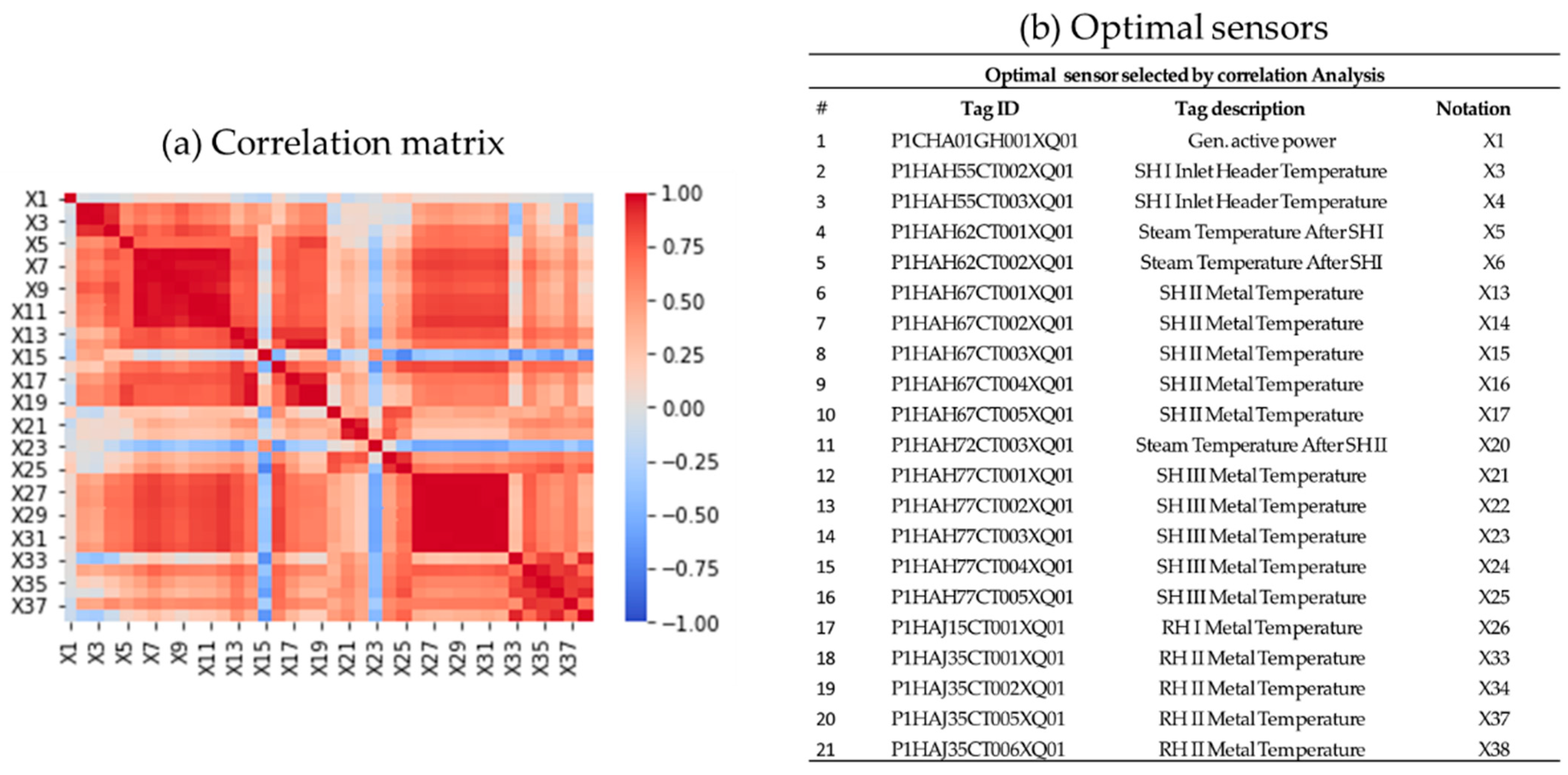
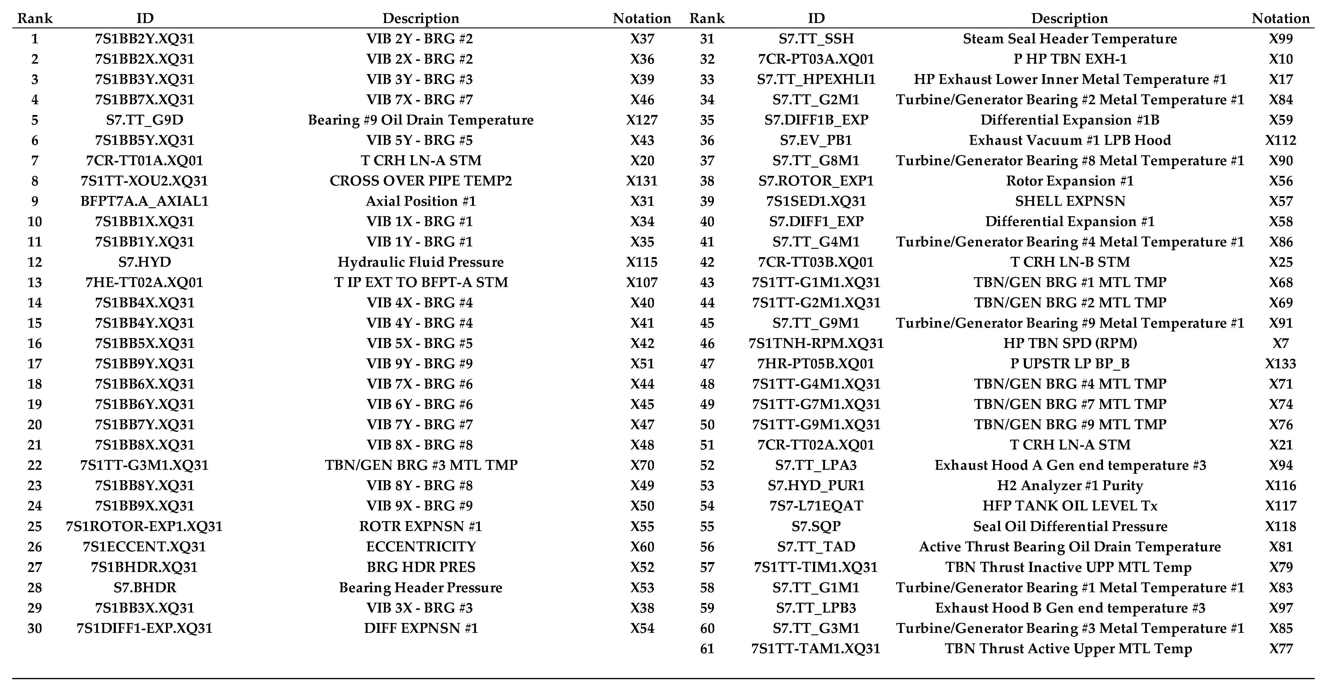
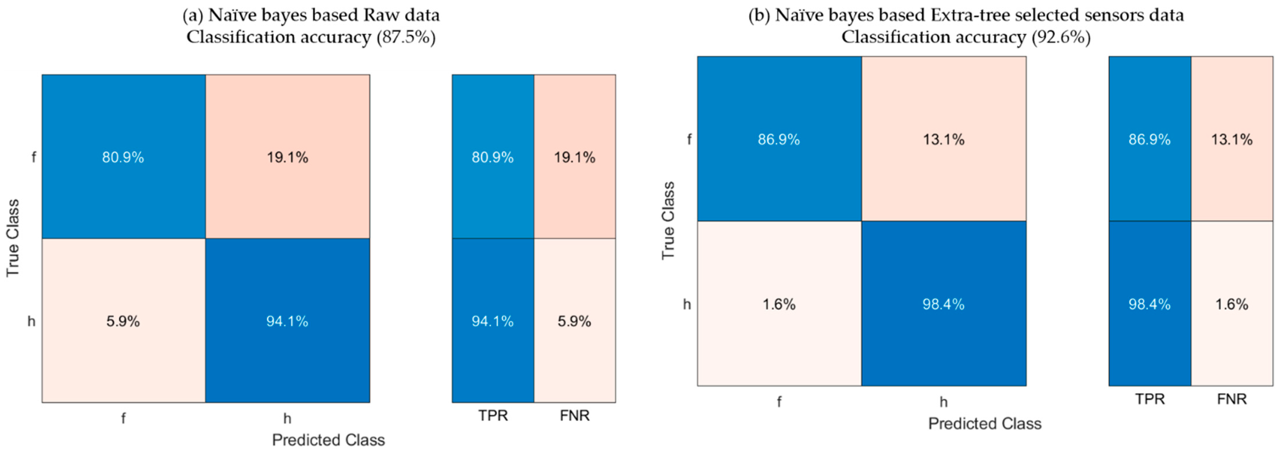
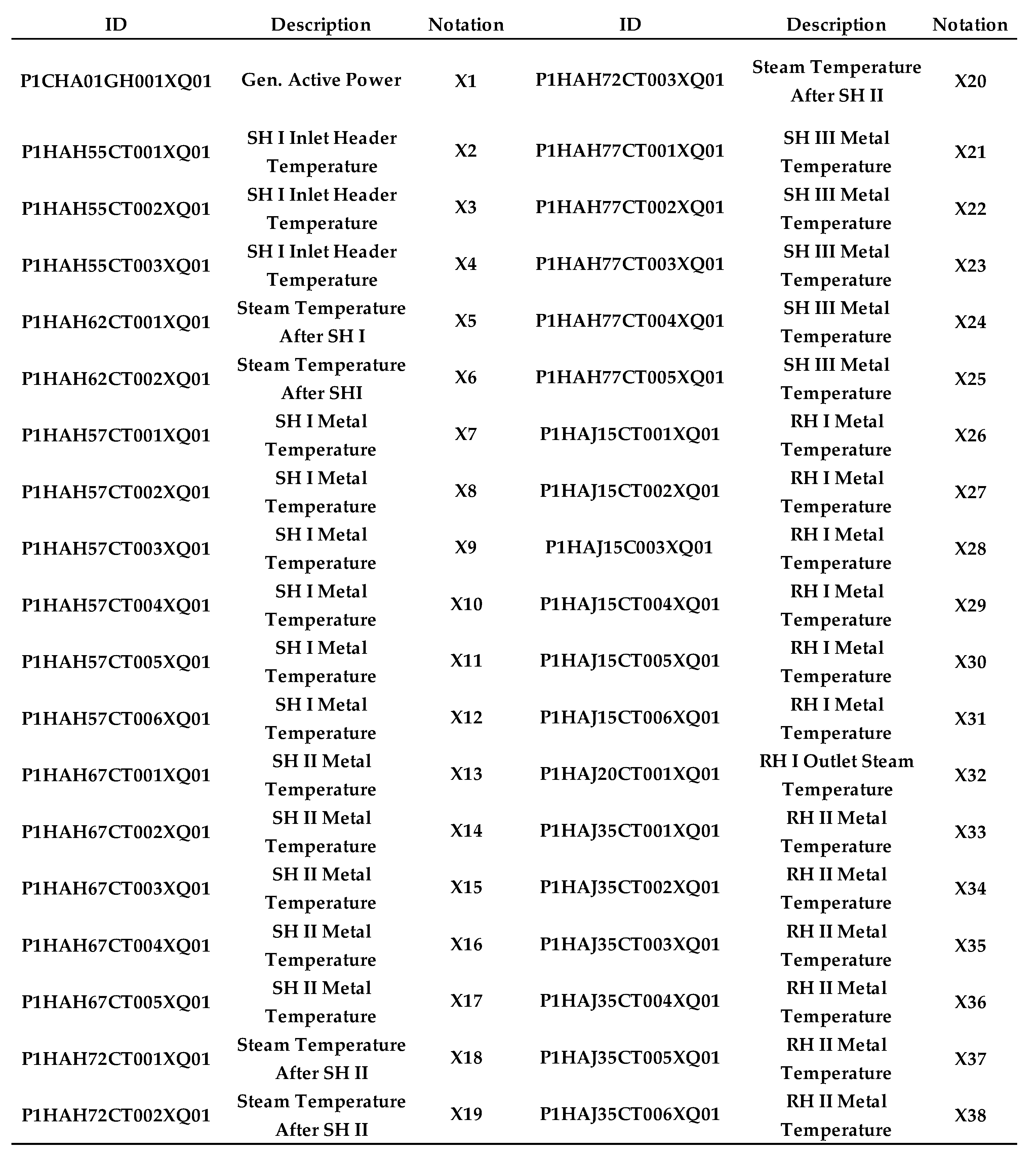
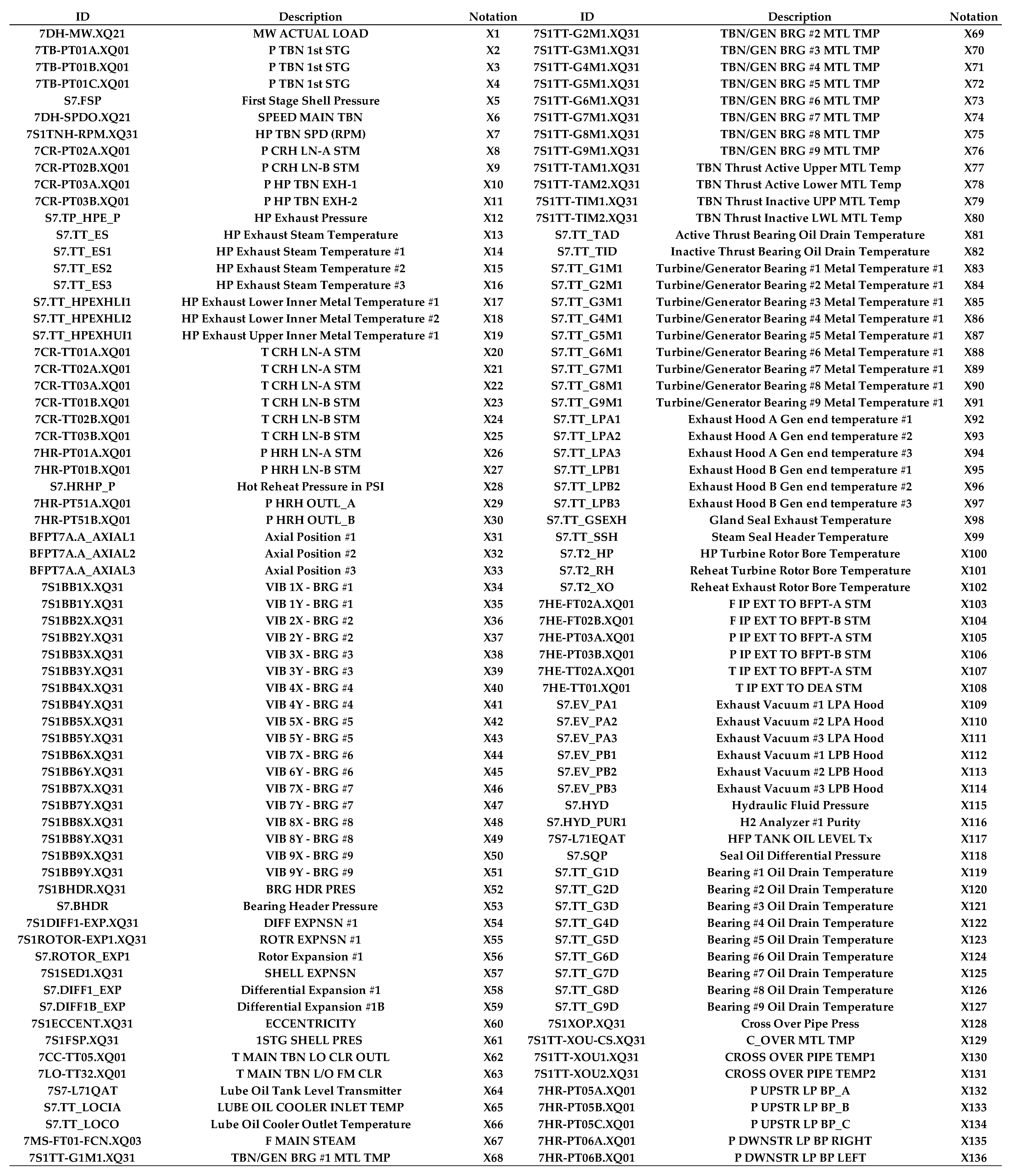
A vast number of sensor data was collected from the historical database of power plants. It is essential to point out the informative sensors necessary to detect the fault in the presence of irrelevant and redundant sensors. Multivariate algorithms are highly dependent on the number of input sensors. The redundant and irrelevant sensors may reduce the performance of these classifiers. Therefore, this study proposed a machine-learning-based optimal sensor selection approach for equipment (boiler and turbine) fault detection in thermal power plants. Three optimal sensor selection approaches (correlation analysis, mRMR algorithm, and extra-tree classifier) are employed in this study. Three supervised machine-learning classifiers (SVM, k-NN, and naïve Bayes) are used to classify the normal and faulty states. The proposed approach is implemented on the two real-world case scenarios (boiler water wall tube leakage and turbine motor fault). The computational results indicate that the optimal sensor selection approaches not only reduced the number of sensors by up to 44% in the water wall tube leakage scenario from 38 to 21 sensors, and by 55% in the turbine fault case scenario from 136 to 61 sensors, but also enhanced the machine-learning accuracy. The k-NN-based mRMR algorithm provides the highest accuracy of up to 97.6% in the boiler water wall tube leakage case scenario. In the second case scenario (turbine motor failure), the naïve-Bayes-based extra-tree classifier provides the highest accuracy of 92.6% compared with the other comparative models. This study suggests the efficient and straightforward optimal sensor selection approaches that can be implemented in thermal power plants, and in future research work, this may provide the guidelines for efficient fault detection in TPPs.

References

1. Basu, S.; Debnath, A.K. Power Plant Instrumentation and Control Handbook: A Guide to Thermal Power Plants; Academic Press: Cambridge, MA, USA, 2015; ISBN 978-0-12-800940-6. [Google Scholar]
2. Zhang, S.; Shen, G.; An, L. Leakage location on water-cooling wall in power plant boiler based on acoustic array and a spherical interpolation algorithm. Appl. Therm. Eng. 2019, 152, 551–558. [Google Scholar] [CrossRef]
3. An, L.; Wang, P.; Sarti, A.; Antonacci, F.; Shi, J. Hyperbolic boiler tube leak location based on quaternary acoustic array. Appl. Therm. Eng. 2011, 31, 3428–3436. [Google Scholar] [CrossRef]
4. Khalid, S.; Lim, W.; Kim, H.S.; Oh, Y.T.; Youn, B.D.; Kim, H.-S.; Bae, Y.-C. Intelligent Steam Power Plant Boiler Waterwall Tube Leakage Detection via Machine Learning-Based Optimal Sensor Selection. Sensors 2020, 20, 6356. [Google Scholar] [CrossRef]
5. Singh, P.M.; Mahmood, J. Stress Assisted Corrosion of Waterwall Tubes in Recovery Boiler Tubes: Failure Analysis. J. Fail. Anal. Prev. 2007, 7, 361–370. [Google Scholar] [CrossRef]
6. Liu, S.; Wang, W.; Liu, C. Failure analysis of the boiler water-wall tube. Case Stud. Eng. Fail. Anal. 2017, 9, 35–39. [Google Scholar] [CrossRef]
7. Yang, P.; Liu, S.S. Fault Diagnosis for Boilers in Thermal Power Plant by Data Mining. In Proceedings of the ICARCV 2004 8th Control, Automation, Robotics and Vision Conference, Kunming, China, 6–9 December 2004; Volume 3, pp. 2176–2180. [Google Scholar]
8. Fortuna, L.; Graziani, S.; Rizzo, A.; Xibilia, M.G. Soft Sensors for Monitoring and Control of Industrial Processes; Advances in Industrial Control; Springer: London, UK, 2007; ISBN 978-1-84628-479-3. [Google Scholar]
9. Yu, J.; Yoo, J.; Jang, J.; Park, J.H.; Kim, S. A novel plugged tube detection and identification approach for final super heater in thermal power plant using principal component analysis. Energy 2017, 126, 404–418. [Google Scholar] [CrossRef]
10. Indrawan, N.; Shadle, L.J.; Breault, R.W.; Panday, R.; Chitnis, U.K. Data analytics for leak detection in a subcritical boiler. Energy 2020, 220, 119667. [Google Scholar] [CrossRef]
11. Swiercz, M.; Mroczkowska, H. Multiway PCA for Early Leak Detection in a Pipeline System of a Steam Boiler—Selected Case Studies. Sensors 2020, 20, 1561. [Google Scholar] [CrossRef] [PubMed] [Green Version]
12. Bhatt, M.S.; Rajkumar, N. Performance Enhancement in Coal Fired Thermal Power Plants. Part II: Steam Turbines. Int. J. Energy Res. 1999, 27, 489–515. [Google Scholar] [CrossRef]
13. Dhini, A.; Kusumoputro, B.; Surjandari, I. Neural Network Based System for Detecting and Diagnosing Faults in Steam Turbine of Thermal Power Plant. In Proceedings of the 2017 IEEE 8th International Conference on Awareness Science and Technology (iCAST), Taichung, China, 8–10 November 2017; pp. 149–154. [Google Scholar]
14. Salahshoor, K.; Khoshro, M.S.; Kordestani, M. Fault detection and diagnosis of an industrial steam turbine using a distributed configuration of adaptive neuro-fuzzy inference systems. Simul. Model. Pr. Theory 2011, 19, 1280–1293. [Google Scholar] [CrossRef]
15. Zhang, X.; Chen, S.; Zhu, Y.; Yan, W. Fault Detection and Diagnosis for Steam Turbine Based on Kernel GDA. In Proceedings of the 2011 International Conference on Modelling, Identification and Control, Shanghai, China, 26–29 June 2011; pp. 58–62. [Google Scholar]
16. Lin, T.-H.; Wu, S.-C. Sensor fault detection, isolation and reconstruction in nuclear power plants. Ann. Nucl. Energy 2018, 126, 398–409. [Google Scholar] [CrossRef]
17. Han Kim, K.; Seok Lee, H.; Hwan Kim, J.; Park, J.H. Detection of Boiler Tube Leakage Fault in a Thermal Power Plant Using Machine Learning Based Data Mining Technique. In Proceedings of the 2019 IEEE International Conference on Industrial Technology (ICIT), Melbourne, Australia, 13–15 February 2019; pp. 1006–1010. [Google Scholar]
18. Jing, C.; Hou, J. SVM and PCA based fault classification approaches for complicated industrial process. Neurocomputing 2015, 167, 636–642. [Google Scholar] [CrossRef]
19. Li, W.; Peng, M.; Wang, Q. Fault identification in PCA method during sensor condition monitoring in a nuclear power plant. Ann. Nucl. Energy 2018, 121, 135–145. [Google Scholar] [CrossRef]
20. Young-Hun kim, J.K. Leakage Detection of a Boiler Tube Using a Genetic Algorithm-like Method and Support Vector Machines. In Proceedings of the Tenth International Conference on Soft Computing and Pattern Recognition (SoCPaR 2018), Porto, Portugal, 13–15 December 2018. [Google Scholar] [CrossRef]
21. Tariq, R.; Hussain, Y.; Sheikh, N.; Afaq, K.; Ali, H.M. Regression-Based Empirical Modeling of Thermal Conductivity of CuO-Water Nanofluid using Data-Driven Techniques. Int. J. Thermophys. 2020, 41, 1–28. [Google Scholar] [CrossRef]
22. Sugumaran, V.; Muralidharan, V.; Ramachandran, K. Feature selection using Decision Tree and classification through Proximal Support Vector Machine for fault diagnostics of roller bearing. Mech. Syst. Signal Process. 2007, 21, 930–942. [Google Scholar] [CrossRef]
23. Chen, K.-Y.; Chen, L.-S.; Chen, M.-C.; Lee, C.-L. Using SVM based method for equipment fault detection in a thermal power plant. Comput. Ind. 2011, 62, 42–50. [Google Scholar] [CrossRef]
24. Radovic, M.D.; Ghalwash, M.F.; Filipovic, N.; Obradovic, Z. Minimum redundancy maximum relevance feature selection approach for temporal gene expression data. BMC Bioinform. 2017, 18, 1–14. [Google Scholar] [CrossRef] [Green Version]
25. Sharaff, A.; Gupta, H. Extra-Tree Classifier with Metaheuristics Approach for Email Classification. In Advances in Computer Communication and Computational Sciences; Bhatia, S.K., Tiwari, S., Mishra, K.K., Trivedi, M.C., Eds.; Advances in Intelligent Systems and Computing; Springer: Singapore, 2019; Volume 924, pp. 189–197. ISBN 9789811368608. [Google Scholar]
26. Sun, X.; Chen, A.T.; Marquez, H.J. Boiler Leak Detection Using a System Identification Technique. Ind. Eng. Chem. Res. 2002, 41, 5447–5454. [Google Scholar] [CrossRef]
27. Afgan, N.; Coelho, P.; Carvalho, M.D.G. Boiler tube leakage detection expert system. Appl. Therm. Eng. 1998, 18, 317–326. [Google Scholar] [CrossRef]
28. Sun, X.; Marquez, H.J.; Chen, T.; Riaz, M. An improved PCA method with application to boiler leak detection. ISA Trans. 2005, 44, 379–397. [Google Scholar] [CrossRef]
29. Lang, F.D.; Rodgers, D.A.T.; Mayer, L.E. Detection of tube leaks and their location using input/loss methods. In Proceedings of the ASME Power Conference, Baltimore, MD, USA, 30 March–1 April 2004; Volume 41626, pp. 143–150. [Google Scholar]
30. Nozari, H.A.; Shoorehdeli, M.A.; Simani, S.; Banadaki, H.D. Model-based robust fault detection and isolation of an industrial gas turbine prototype using soft computing techniques. Neurocomputing 2012, 91, 29–47. [Google Scholar] [CrossRef]
31. Liu, Y.; Su, M. Nonlinear Model Based Diagnostic of Gas Turbine Faults: A Case Study. In Proceedings of the Volume 3: Controls, Diagnostics and Instrumentation; Education; Electric Power; Microturbines and Small Turbomachinery; Solar Brayton and Rankine Cycle (ASMEDC), Vancouver, BC, Canada, 1 January 2011; pp. 1–8. [Google Scholar]
32. Ismail, F.B.; Singh, D.; Maisurah, N.; Musa, A.B.B. Early tube leak detection system for steam boiler at KEV power plant. MATEC Web Conf. 2016, 74, 6. [Google Scholar] [CrossRef] [Green Version]
33. Bhatt, M.S.; Jothibasu, S. Performance Enhancement in Coal Fired Thermal Power Plants. Part I: Boilers. Int. J. Energy Res. 1999, 23, 1239–1266. [Google Scholar] [CrossRef]
34. Kokkinos, A. Coal R&D Beyond 2020. DOE-NETL-EPRI Technical Exchange Meeting; EPRI: Pittsburgh, PA, USA, 2019. [Google Scholar]
35. Yong, S.; Lin, M.; Robinson, W.; Fidge, C. Using Decision Trees in Economizer Repair Decision Making. In Proceedings of the 2010 Prognostics and System Health Management Conference, Macao, China, 12–14 January 2010; pp. 1–6. [Google Scholar]
36. Liu, K.; Feng, X.; Ma, K.; Wang, L.; Xie, X.; Lu, Z. Investigation on the welding-induced multiple failures in boiler water wall tube. Eng. Fail. Anal. 2020, 121, 104988. [Google Scholar] [CrossRef]
37. Yang, G.; Gou, Y.; Liu, X.; Zhang, X.; Zhang, T. Failure Analysis of the Corroded Water Wall Tube in a 50MW Thermal Power Plant. High Temp. Mater. Process. 2018, 37, 995–999. [Google Scholar] [CrossRef]
38. Xue, S.; Guo, R.; Hu, F.; Ding, K.; Liu, L.; Zheng, L.; Yang, T. Analysis of the causes of leakages and preventive strategies of boiler water-wall tubes in a thermal power plant. Eng. Fail. Anal. 2020, 110, 104381. [Google Scholar] [CrossRef]
39. Tanuma, T. Introduction to steam turbines for power plants. In Advances in Steam Turbines for Modern Power Plants; Elsevier: Amsterdam, The Netherlands, 2017; pp. 3–9. ISBN 978-0-08-100314-5. [Google Scholar]
40. Nagar, A.; Mehta, S. Steam Turbine Lube Oil System Protections Using SCADA & PLC. In Proceedings of the 2017 International Conference on Intelligent Computing and Control Systems (ICICCS), Madurai, India, 15–16 June 2017; pp. 1376–1381. [Google Scholar]
41. Dias, C.G.; Pereira, F.H. Broken Rotor Bars Detection in Induction Motors Running at Very Low Slip Using a Hall Effect Sensor. IEEE Sens. J. 2018, 18, 4602–4613. [Google Scholar] [CrossRef]
42. Niu, J.; Lu, S.; Liu, Y.; Zhao, J.; Wang, Q. Intelligent Bearing Fault Diagnosis Based on Tacholess Order Tracking for a Variable-Speed AC Electric Machine. IEEE Sens. J. 2018, 19, 1850–1861. [Google Scholar] [CrossRef]
43. Fu, Q.; Jing, B.; He, P.; Si, S.; Wang, Y. Fault Feature Selection and Diagnosis of Rolling Bearings Based on EEMD and Optimized Elman_AdaBoost Algorithm. IEEE Sens. J. 2018, 18, 5024–5034. [Google Scholar] [CrossRef]
44. Rao, S.G.; Lohith, S.; Gowda, P.C.; Singh, A.; Rekha, S.N. Fault Analysis of Induction Motor. In Proceedings of the 2019 IEEE International Conference on Intelligent Techniques in Control, Optimization and Signal Processing (INCOS), Tamilnadu, India, 11–13 April 2019; pp. 1–4. [Google Scholar]
45. Moradi, M.; Chaibakhsh, A.; Ramezani, A. An intelligent hybrid technique for fault detection and condition monitoring of a thermal power plant. Appl. Math. Model. 2018, 60, 34–47. [Google Scholar] [CrossRef]
46. Shaheryar, A.; Yin, X.-C.; Hao, H.-W.; Ali, H.; Iqbal, K. A Denoising Based Autoassociative Model for Robust Sensor Monitoring in Nuclear Power Plants. Sci. Technol. Nucl. Install. 2016, 2016, 1–17. [Google Scholar] [CrossRef] [Green Version]
47. Yoshizawa, T.; Hirobayashi, S.; Misawa, T. Noise reduction for periodic signals using high-resolution frequency analysis. EURASIP J. Audio Speech Music. Process. 2011, 2011, 5. [Google Scholar] [CrossRef] [Green Version]
48. Curling, L.; Gagnon, J.; Paidoussis, M. Noise removal from power spectral densities of multicomponent signals by the coherence method. Mech. Syst. Signal Process. 1992, 6, 17–27. [Google Scholar] [CrossRef]
49. Abbasi, A.R.; Rafsanjani, A.; Farshidianfar, A.; Irani, N. Rolling element bearings multi-fault classification based on the wavelet denoising and support vector machine. Mech. Syst. Signal Process. 2007, 21, 2933–2945. [Google Scholar] [CrossRef]
50. Wang, Z.; Zhang, Q.; Xiong, J.; Xiao, M.; Sun, G.; He, J. Fault Diagnosis of a Rolling Bearing Using Wavelet Packet Denoising and Random Forests. IEEE Sens. J. 2017, 17, 5581–5588. [Google Scholar] [CrossRef]
51. Risqiwati, D.; Wibawa, A.D.; Pane, E.S.; Islamiyah, W.R.; Tyas, A.E.; Purnomo, M.H. Feature Selection for EEG-Based Fatigue Analysis Using Pearson Correlation. In Proceedings of the 2020 International Seminar on Intelligent Technology and Its Applications (ISITIA), Surabaya, Indonesia, 22–23 July 2020; pp. 164–169. [Google Scholar]
52. Benesty, J.; Chen, J.; Huang, Y.; Cohen, I. Pearson Correlation Coefficient. In Noise Reduction in Speech Processing; Springer Topics in Signal Processing; Springer: Berlin/Heidelberg, Germany, 2009; Volume 2, pp. 1–4. ISBN 978-3-642-00295-3. [Google Scholar]
53. Peng, H.; Long, F.; Ding, C. Feature selection based on mutual information criteria of max-dependency, max-relevance, and min-redundancy. IEEE Trans. Pattern Anal. Mach. Intell. 2005, 27, 1226–1238. [Google Scholar] [CrossRef] [PubMed]
54. Yan, X.; Jia, M. Intelligent fault diagnosis of rotating machinery using improved multiscale dispersion entropy and mRMR feature selection. Knowl.-Based Syst. 2018, 163, 450–471. [Google Scholar] [CrossRef]
55. Stetco, A.; Dinmohammadi, F.; Zhao, X.; Robu, V.; Flynn, D.; Barnes, M.; Keane, J.; Nenadic, G. Machine learning methods for wind turbine condition monitoring: A review. Renew. Energy 2018, 133, 620–635. [Google Scholar] [CrossRef]
56. Jack, L.; Nandi, A. Fault detection using support vector machines and artificial neural networks, augmented by genetic algorithms. Mech. Syst. Signal Process. 2002, 16, 373–390. [Google Scholar] [CrossRef]
57. Guenther, N.; Schonlau, M. Support Vector Machines. Stata J. Promot. Commun. Stat. Stata 2016, 16, 917–937. [Google Scholar] [CrossRef] [Green Version]
58. Yuan, J.; Wang, C.; Zhou, Z. Study on refined control and prediction model of district heating station based on support vector machine. Energy 2019, 189, 116193. [Google Scholar] [CrossRef]
59. Vernekar, K.; Kumar, H.; Gangadharan, K.V. Engine gearbox fault diagnosis using empirical mode decomposition method and Naïve Bayes algorithm. Sadhana 2017, 42, 1143–1153. [Google Scholar] [CrossRef] [Green Version]
60. Schmidt, J.; Marques, M.R.G.; Botti, S.; Marques, M.A.L. Recent advances and applications of machine learning in solid-state materials science. NPJ Comput. Mater. 2019, 5. [Google Scholar] [CrossRef]
Figure 1. Essential equipment in a coal-fired TPP.
Mathematics 09 02814 g001
Figure 2. Survey of power plant faults representing the severity of the power plant faults and outage percentages.
Mathematics 09 02814 g002
Figure 3. Schematic of the overall methodology.
Mathematics 09 02814 g003
Figure 4. P&ID diagram of the LP turbine section in a TPP.
Mathematics 09 02814 g004
Figure 5. Detailed summary of the proposed approach.
Mathematics 09 02814 g005
Figure 6. Thermocouple sensors data showing the healthy (normal) and the leakage state of the boiler with the corresponding generator active power.
Mathematics 09 02814 g006
Figure 7. The noisy and denoised sensor signal showing the effectiveness of the wavelet denoising.
Mathematics 09 02814 g007
Figure 8. (a) Correlation between the input sensors; (b) the optimal sensors selected after correlation analysis.
Mathematics 09 02814 g008
Figure 9. (a) mRMR algorithm selected sensors; (b) optimal sensors selected by mRMR algorithm.
Mathematics 09 02814 g009
Figure 10. (a) Extra-tree classifier selected sensors; (b) optimal sensors selected by the extra-tree classifier.
Mathematics 09 02814 g010
Figure 11. Machine-learning performance comparison of the four data case scenarios.
Mathematics 09 02814 g011
Figure 12. (a) Confusion matrix for the k-NN-based raw data case scenario; (b) confusion matrix for the k-NN-based mRMR algorithm case scenario.
Mathematics 09 02814 g012
Figure 13. Sensor data showing the healthy (normal) and the faulty state of the steam turbine with the corresponding generator active power.
Mathematics 09 02814 g013
Figure 14. Wavelet denoising of the noisy data.
Mathematics 09 02814 g014
Figure 15. Correlation matrix of the sensitive sensor data.
Mathematics 09 02814 g015
Figure 16. List of the optimal sensors selected by correlation analysis.
Mathematics 09 02814 g016
Figure 17. Optimal sensors ranking with the predictor importance score.
Mathematics 09 02814 g017
Figure 18. List of optimal sensors selected by mRMR algorithm.
Mathematics 09 02814 g018
Figure 19. Optimal sensor ranking with the predictor importance score.
Mathematics 09 02814 g019
Figure 20. List of optimal sensors selected by extra-tree algorithm.
Mathematics 09 02814 g020
Figure 21. Machine-learning performance comparison of the four data case scenarios.
Mathematics 09 02814 g021
Figure 22. (a) Confusion matrix for the naïve-Bayes-based raw data case scenario; (b) confusion matrix for the naïve-Bayes-based extra-tree classifier case scenario.
Mathematics 09 02814 g022