Modelling Short- and Long-Term Dependencies of Clustered High-Threshold Exceedances in Significant Wave Heights

Abstract

The peaks-over-threshold (POT) method has a long tradition in modelling extremes in environmental variables. However, it has originally been introduced under the assumption of independently and identically distributed (iid) data. Since environmental data often exhibits a time series structure, this assumption is likely to be violated due to short- and long-term dependencies in practical settings, leading to clustering of high-threshold exceedances. In this paper, we first review popular approaches that either focus on modelling short- or long-range dynamics explicitly. In particular, we consider conditional POT variants and the Mittag–Leffler distribution modelling waiting times between exceedances. Further, we propose a new two-step approach capturing both short- and long-range correlations simultaneously. We suggest the autoregressive fractionally integrated moving average peaks-over-threshold (ARFIMA-POT) approach, which in a first step fits an ARFIMA model to the original series and then in a second step utilises a classical POT model for the residuals. Applying these models to an oceanographic time series of significant wave heights measured on the Sefton coast (UK), we find that neither solely modelling short- nor long-range dependencies satisfactorily explains the clustering of extremes. The ARFIMA-POT approach, however, provides a significant improvement in terms of model fit, underlining the need for models that jointly incorporate short- and long-range dependence to address extremal clustering, and their theoretical justification.

1. Introduction

Extreme value theory (EVT) has emerged as an invaluable toolkit for a broad range of sciences in recent decades. It attempts to predict the occurrence of extreme events by making the best use of limited available data. They can be divided into two fundamental approaches: the block maxima method and the peaks-over-threshold (POT) method, while the former splits the observation period into non-overlapping, equally-sized periods and then only analyses the maximum of each period, the latter picks extreme observations exceeding a specific high threshold [1]. In the following, we focus on the POT method, which has proven useful in a variety of applications including financial risk management [2,3], insurance [4], coastal engineering [5,6], and oceanography [7,8]. We regard the POT approach from the perspective of a marked point process (MPP): exceedances over a high threshold u will be referred to as extreme events. Such an event is associated with an occurrence time and a mark size, the latter corresponding to the size of the excess above the threshold.

The motivation for the classical POT model can be found in the asymptotic behaviour of high threshold exceedances for identically and independently distributed (iid) data. The approach assumes that if the threshold u is chosen high enough, the extreme events follow a marked Poisson process, i.e., the number of extremes events occurring can be described by a homogeneous Poisson process and their mark sizes are iid with a generalised Pareto distribution (GPD). This process also characterises the inter-event times as being iid exponentially distributed.

In many practical settings, however, the iid assumption is violated. Short-range dependencies arising from local serial correlation of the underlying time series may cause extreme events to occur in clusters [2]. Therefore, assuming independent exponential inter-event times may seem unreasonable. These practical issues are often tackled by using declustering methods and then fitting the marked Poisson process to the largest value of each cluster only (see, e.g., [9]). This approach however disregards the information contained within the clusters (cf. [10,11]), and gives rise to the challenge of appropriately and consistently identifying clusters from given data. Relevant literature includes works on statistical declustering using the extremal index due to Leadbetter et al. [10,12,13,14,15], on physical declustering [10,16,17], or on double threshold approaches combining statistical and physical declustering [18,19]. However, all these declustering methods have in common that they avoid modelling the short-range dependence directly.

It is impossible to universally characterise the short-term behaviour of stationary sequences as it can take countless different forms, but imposing certain constraints on the local dependence structure enables parametric modelling thereof. One approach builds on a marked point process with a self-exciting structure to model the clustering of extreme events, leading to conditional POT approaches. The Hawkes-POT model introduced by Chavez-Demoulin et al. [2] belongs to the general class of self-exciting Hawkes processes [20] and allows the intensity of the occurrence of extreme events to depend on both past event times and marks. A related approach is the so-called self-exciting POT (SEPOT) suggested by McNeil et al. [21], where one Hawkes process influences the intensity of both event times and marks. The various conditional POT models were reviewed in [3,22,23,24], and extended to a multivariate framework by Grothe et al. [25] and Hautsch and Herrera [26]. Conditional POT models are based on similar ideas as the epidemic-type aftershock sequence (ETAS) model proposed by Ogata [27], which is designed to describe the occurrence of earthquakes based on previous ones and was further explored for example by Helmstetter and Sornette [28].

In the aforementioned approaches, the conditional intensities of the events depend exponentially on the characteristics of past events implying a focus on modelling short-term dependencies explicitly, but neglecting any possible long-term correlations. However, we also have to consider settings in which long-range dependence in the underlying sequence influences the clustering behaviour so that we cannot per se assume that widely separated events are independent. Many time series of practical interest ranging from finance [29] to hydrology [30] and forestry [31] have long been known to exhibit long-range dependence, implying a power-like decay of the autocovariance function $\gamma \left(h\right)$, $h\in \mathbb{Z}$, i.e.,

$$\gamma \left(h\right)\sim {c\left|h\right|}^{2d-1}\mathrm{as}h\to \infty$$

(1)

where $c>0$ and $0<d<0.5$ for a stationary process [32]. An alternative definition is based on the spectral density $f\left(\lambda \right)=\frac{1}{2\pi }{\sum }_{h=-\infty }^{\infty }\gamma \left(h\right)exp\left(-ih\lambda \right)$ with $\lambda \in [-\pi ,\pi ]$. The spectral density of a long-range dependent series has a pole at the origin and decays hyperbolically thereafter, i.e., the spectral density is described by

$$f\left(\lambda \right)\sim {c\left|\lambda \right|}^{-2d}\mathrm{as}\lambda \to 0$$

(2)

where $c>0$ and $0<d<0.5$ [33].

Modelling the extreme events of long-range dependent time series hence requires special attention to the characteristics that event times and marks inherit from the underlying process. Generally, long-range dependence in the underlying time series has been observed to lead to pronounced clustering of extreme events [34,35]. There is empirical evidence that the inter-event times may follow a Weibull [36], a stretched exponential distribution [37,38,39] or the product of a power law and a stretched exponential [40], but these observations lack analytical justification. The inter-event times themselves have also been found to exhibit long-range dependence [35,41]. In numerical experiments, maxima sequences were as well found to exhibit long-range dependence and, depending on the distribution and the strength of the long-term correlations of the underlying sequence, the distribution of maxima may deviate from the asymptotics for finite block sizes [42]. It could be suspected that the effects on the whole tail of the mark distribution might be more pronounced than when considering only a sequence of maxima.

In the context of EVT, not many parametric approaches exist that incorporate explicit modelling of the long-term dependence structure in the underlying series. One example is suggested by Hees et al. [43] and motivated by so-called bursty extremes where event clusters are separated by long periods without any event. Hees et al. [43] provide a parametric approach to modelling a setting in which the event occurrences follow a fractional Poisson process which was proved to be long-range dependent by Biard and Saussereau [44]. They focus on characterising the inter-event times via the Mittag–Leffler distribution, which generalises the exponential distribution [45,46]. This framework can easily be complemented by additionally modelling the mark sizes through a GPD [43].

All these variants of the POT model have in common that they explicitly model the dependence structure of the underlying times series to capture the clustering behaviour of the extreme events, either by taking into account short-term or long-term correlations. However, none of the models embeds short- and long-range dynamics at the same time. Considering real world applications, it is very likely that many financial and physical processes are governed by both short- and long-range dependencies affecting the cluster formation of their extreme events.

The focus of this paper lies on oceanographic variables which are frequently identified to be long-range dependent. Especially near the coast, sea level observations [47,48] and sea surface temperatures [49,50] were found to exhibit long-range dependence. Similar findings are reported for sea-ice thickness [51] and significant wave height [52,53,54]. The dataset we consider in our application in Section 4 also consists of significant wave heights that were measured on the Sefton coast (UK). 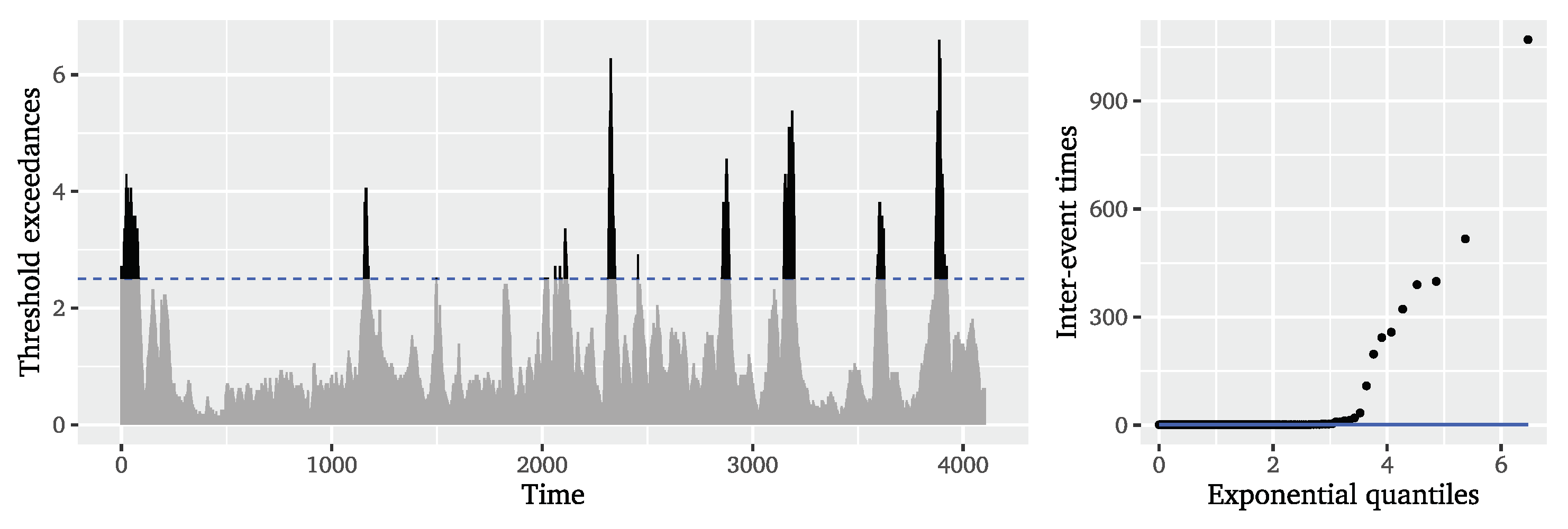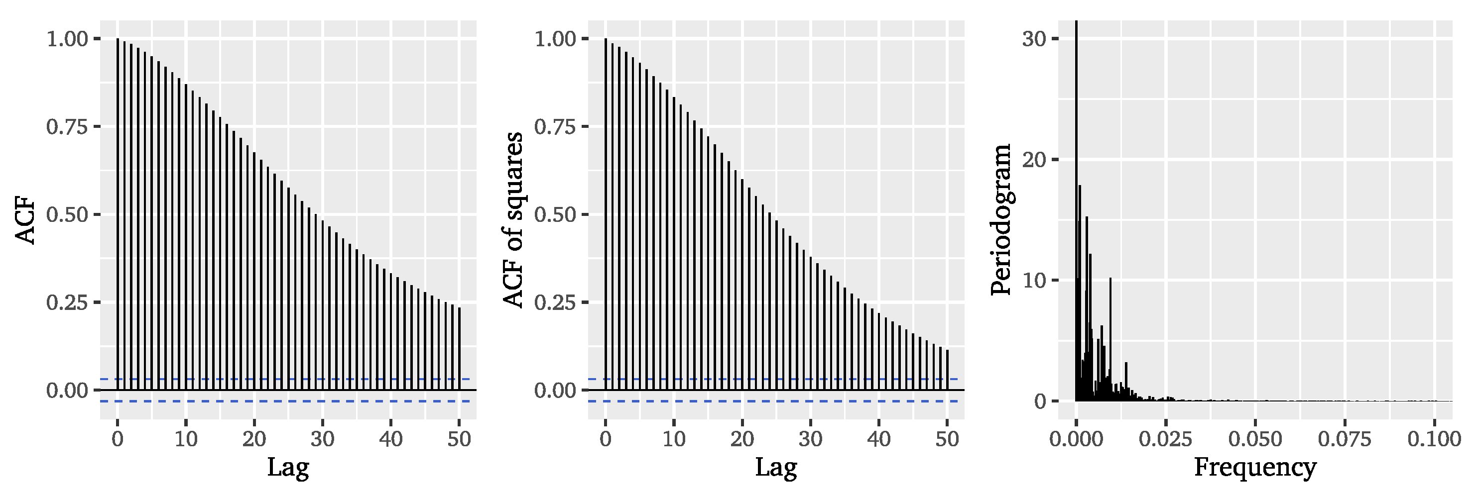Figure 1 depicts the observed time series and illustrates the exceedances of the high threshold $u=2.5$ m, i.e., the extreme events. It is obvious that the extreme events appear in widely separated clusters implying strong local dependencies, which is confirmed by the empirical autocorrelation functions (ACFs) of both observations and their squares (cf. Figure 2). Therefore, it is not surprising that the inter-event times appear to have a distribution clearly differing from the exponential distribution expected for iid observations, as can be observed from the quantile-quantile (QQ) plot in Figure 1. The periodogram of the significant wave heights in Figure 2 further hints at the presence of long-range dependence due to the pole at the origin, which is in line with the aforementioned literature.

Thus, the visual inspection of the considered dataset implies that the dependence structure of the significant wave heights exhibits both short- and long-term correlations. Of course this has to be accounted for when attempting to explicitly characterise the extremal clustering.

Therefore, with the aim of jointly modelling short- and long-range dependencies, we suggest a two-step approach in the spirit of McNeil and Frey [55] which we will call autoregressive fractionally integrated moving average peaks-over-threshold (ARFIMA-POT) approach. Addressing the issue of heteroscedasticity in financial data, McNeil and Frey [55] introduced the so-called GARCH-EVT approach which first fits a GARCH model to a return series and then applies standard EVT techniques to the pseudo-iid residuals from the first step. Even though there is no theory that mathematically characterises the clustering behaviour of the extremes from GARCH model residuals [56], the two-stage method has proven to work well in practice [57,58,59,60,61]. In a similar fashion, we propose a two-stage method combining a parametric model with a classical EVT model.

Our ARFIMA-POT approach is based on first fitting an autoregressive fractionally integrated moving average (ARFIMA) model [62,63] to the original oceanographic dataset and then applying the standard POT model to the ARFIMA residuals. Given that the ARFIMA model captures both short- and long-range dependence in the underlying time series, the model residuals are supposed to be iid, so that all difficulties arising for the distribution of event times and mark sizes due to the short- and long-term behaviour in the original series can be avoided. The method is inspired by the idea of prewhitening the underlying series as suggested for example by Davison and Smith [9] to deal with non-stationarity and seasonality in POT modelling. For Hill’s estimator of the tail index, Resnick and Stărică [64,65] show that using the residuals of an autoregressive (AR) process is superior in terms of asymptotic variance than estimation based directly on the observations, given that the series follows an AR process and the AR model has a causal representation. This clearly indicates that prewhitening can have favourable properties in the context of EVT. Further, the idea of utilising an ARFIMA model to describe a time series in the context of oceanography is not new. ARFIMA models are a popular choice for characterising levels and trends in weather-related, hydrological and oceanographic data [66]. Specifically, Ercan at al. [48] for instance model the Caspian sea level using ARFIMA processes. Thus, our ARFIMA-POT approach can be interpreted as filtering the underlying oceanographic time series using an ARFIMA model before applying the classical POT method.

This paper contributes to the line of literature that aims to model the clustering behaviour of extreme events. Specifically, we consider strongly dependent significant wave height data for which high level exceedances appear in an extremely clustered manner. As this setting poses a particular challenge for traditional POT approaches, we analyse whether popular models dealing with short- or long-range dependence convey enough information about the dependence structure in the data. Moreover, we suggest the two-step ARFIMA-POT approach that captures both short- and long-range dependence in the underlying time series. Further, we verify our conclusions from the application to significant wave heights in a simulation study. The range of models reviewed is not meant to be exhaustive, but is rather supposed to present a selection of commonly used approaches modelling either the short- or long-term behaviour of extreme events, but not both simultaneously. Our results are meant to provide a basis for further discourse on the modelling of extremal clustering behaviour in EVT. We show that current tools are not flexible enough to simultaneously capture the short- and long-range dependence of the underlying process. Therefore, we want to spark new interest in researching the intersection of modelling local clustering behaviour and long-range dependence to find solutions to a question of practical interest.

The paper is organised as follows. Section 2 reviews the basic concepts around POT modelling. Section 3 presents the considered models. This section is divided into established models characterising extremal clustering by taking into account short- and long-range dependence, respectively, and the presentation of the two-step ARFIMA-POT approach incorporating short- and long-term dynamics simultaneously. Section 4 applies the considered approaches to significant wave heights and discusses their performance in the presence of extremal clustering and long-range dependence. Section 5 examines the conclusions from the application in a simulation study and Section 6 concludes.

2. Peaks-over-Threshold Modelling

In the following, we review the univariate POT approach through the lens of point processes as introduced by Pickands [67]. In the presentation, we loosely follow McNeil et al. [21].

Consider a sequence of iid random variables $X_1,\cdots ,X_n$ with some continuous distribution function F that is in the maximum domain of attraction of a non-degenerate limiting distribution, i.e., $F\in MDA\left(H_{\xi }\right)$ for some $\xi \in \mathbb{R}$, so that ${lim}_{n\to \infty }n\overline{F}(a_{n}x+b_n)=-ln{H}_{\xi }\left(x\right)$ holds for normalising sequences $a_n>0$ and $b_n$ where $\overline{F}\left(x\right)=1-F\left(x\right)$. It follows that $H_{\xi }$ is a generalised extreme value (GEV) distribution with distribution function

$$H_{\xi }\left(x\right)=\left\{\begin{array}{cc}exp\left(-{\left(1+\xi \frac{x-\mu }{\sigma }\right)}_{+}^{-1/\xi }\right),\hfill & \xi \ne 0,\hfill \\ exp\left(-exp\left(-\frac{x-\mu }{\sigma }\right)\right),\hfill & \xi =0,\hfill \end{array}\right.$$

(3)

where ${(·)}_{+}:=max(0,·)$, and $\mu$, $\xi$, $\sigma >0$ denote location, shape and scale parameters, respectively.

The number of exceedances above a high threshold u can be expressed by $K:=\#\{i\in \{1,\cdots ,n\}:(X_i-b_n)/a_n>u\}$. Since the $X_i$ are iid, K is binomially distributed with parameters $(n,p)$, where p is the probability of crossing u, i.e., $p=P\left((X_i-b_i)/a_n)>u\right)=\overline{F}(a_{n}u+b_n)=-\frac{1}{n}ln{H}_{\xi }\left(u\right)$. Thus, as $n\to \infty$, K converges to a Poisson random variable with mean $\nu \left(u\right)=-ln{H}_{\xi }\left(u\right)$. However, not only the total number of extreme events is asymptotically Poisson, but also their occurrences can be described by a Poisson point process. We can define the point process of event times as $N_{\left(t\right)}\left(A\right)={\sum }_{i=1}^n{\mathrm{𝟙}}_{\{Y_{i,n}\in A\}}$, where $Y_{i,n}=\frac{i}{n}{\mathrm{𝟙}}_{\{X_i>a_{n}u+b_n\}}$ for $1\le i\le n$ is either the time of an event re-scaled to ${\mathcal{X}}_1=(0,1]$ or zero, and $A\subset {\mathcal{X}}_1$. Then $N_{\left(t\right)}$ converges in distribution to a homogeneous Poisson point process on the space ${\mathcal{X}}_1$ with intensity measure $T\left(A\right)=(t_2-t_1)\tau \left(u\right)$ for $A=(t_1,t_2)\subset {\mathcal{X}}_1$, where the constant intensity is given by $\tau \left(u\right)=\tau =-ln{H}_{\xi ,\mu ,\sigma }\left(u\right)$ and the scaling sequences are absorbed into the parameters of H (see, e.g., [14]).

One way to describe the POT model is by means of a non-homogeneous two-dimensional Poisson point process, for which a two-dimensional pattern of points $(t,x)$ is recorded representing the times and magnitudes of exceedances of a high threshold u [21,68]. On a space ${\mathcal{X}}_2=(0,1]\times (u,\infty )$, we assume for $A\subset {\mathcal{X}}_2$ that the point process $N_{(t,x)}\left(A\right)={\sum }_{i=1}^n{\mathrm{𝟙}}_{\{(i/n,X_i)\in A\}}$ is a Poisson process with intensity function

$$\lambda (t,x)=\left\{\begin{array}{cc}\frac{1}{\sigma }{\left(1+\xi \frac{x-\mu }{\sigma }\right)}^{-1/\xi -1},\hfill & \left(1+\xi \frac{x-\mu }{\sigma }\right)>0,\hfill \\ 0,\hfill & \mathrm{otherwise}.\hfill \end{array}\right.$$

(4)

This intensity function does not depend on t, but on x, so that the two-dimensional Poisson process $N_{(t,x)}$ is non-homogeneous. Considering $A=(t_1,t_2)\times (z,\infty )\subset {\mathcal{X}}_2$, the intensity measure of the process is given by

$$\Lambda \left(A\right)={\int }_{t_1}^{t_2}{\int }_z^{\infty }\lambda (t,x)\mathrm{d}x\mathrm{d}t=-(t_2-t_1)ln{H}_{\xi ,\mu ,\sigma }\left(z\right).$$

(5)

It follows that for any $z\ge u$ the implied one-dimensional process of occurrences of exceedances with level z forms a homogeneous Poisson process with intensity $\tau \left(z\right)=-ln{H}_{\xi ,\mu ,\sigma }\left(z\right)$, which is similar to the previous result.

From this representation, we can also retrieve the GPD as the limiting distribution of the mark sizes: the limiting conditional probability that $(X_i-b_n)/a_n>u+v$ given $(X_i-b_n)/a_n>u$, i.e., the tail of the excess distribution function over the threshold u, is obtained from the ratio of the rates of exceeding the levels $u+v$ and u:

$$\frac{\tau (u+v)}{\tau \left(u\right)}={\left(1+\xi \frac{v}{\sigma +\xi (u-\mu )}\right)}^{-1/\xi }={\overline{G}}_{\xi ,\beta }\left(v\right)$$

(6)

for a positive scaling parameter $\beta =\sigma +\xi (u-\mu )$. ${\overline{G}}_{\xi ,\beta }$ exactly corresponds to the tail of the GPD model for excesses of a high threshold u.

Hence, this representation of the POT model incorporates a homogeneous Poisson process when only considering the re-scaled event times $j/n$ and iid marks $Y_j=X_j-u$, following the GPD with distribution function

$$G_{\xi ,\beta }\left(y\right)=\left\{\begin{array}{cc}1-{\left(1+\xi \frac{y}{\beta }\right)}^{-1/\xi },\hfill & \xi \ne 0,\hfill \\ 1-exp\left(-\frac{y}{\beta }\right),\hfill & \xi =0,\hfill \end{array}\right.$$

(7)

so that we can regard this POT model as an MPP.

To fit the POT model, it is sufficient to fit the Poisson point process with the intensity function (4) for $A={\mathcal{X}}_2$. Due to the non-homogeneity of $N_{(t,x)}$, we define $\lambda \left(x\right):=\lambda (t,x)$. Then the likelihood for $N_{(t,x)}\left(A\right):=N^{*}$ exceedances $X_j$ can be formulated as

$$L\left(\xi ,\mu ,\sigma ;X_1,\cdots ,X_{N^{*}}\right)=exp\left(-\tau \left(u\right)\right)\prod _{j=1}^{N^{*}}\lambda \left(X_j\right).$$

(8)

Alternatively, the POT model can be reparameterised using $\tau :=\tau \left(u\right)=-ln{H}_{\xi ,\mu ,\sigma }\left(u\right)$ for the intensity of the one-dimensional Poisson process of event times, and $\beta =\sigma +\xi (u-\mu )$ for the GPD scaling parameter that is implied for the mark sizes. In that case, the intensity function in (4) can be reformulated using the definition $\lambda \left(x\right):=\lambda (t,x)$ and the mark sizes $Y_j=X_j-u$ as

$$\lambda \left(y\right)=\frac{\tau }{\beta }{\left(1+\xi \frac{y}{\beta }\right)}^{-1/\xi -1},$$

(9)

with $\xi \in \mathbb{R}$ and $\tau ,\beta >0$. The logarithm of the likelihood in (8) can then be shown to become

$$lnL\left(\xi ,\sigma ,\mu ;X_1,\cdots ,X_{N^{*}}\right)=ln{L}_1\left(\xi ,\beta ;X_1,\cdots ,X_{N^{*}}\right)+ln{L}_2\left(\tau ;N^{*}\right)$$

(10)

where $L_1$ corresponds to the likelihood of fitting a GPD to the mark sizes and $L_2$ to the likelihood of a one-dimensional homogeneous Poisson process with intensity $\tau$. Thus, we can make inferences about the parameters for each partition of the log-likelihood separately.

In the POT framework, a central question is how to choose the threshold u. Coles [69] suggested a graphical diagnostic based on the criterion of stability domains. The method aims at identifying regions for the shape parameter $\xi$ and the modified scale parameter $\sigma =\beta -\xi u$, in which the estimates remain constant for an increasing u. Mazas and Hamm [18] propose to select the lowest threshold of the highest domain of stability in order to balance the trade off between choosing a high threshold to minimise the bias and choosing a lower threshold to retain enough data for minimising the variance of the estimates.

This classical POT approach relies on the assumption that the underlying series is independent. Leadbetter [70] extended this theory to stationary sequences satisfying certain weak dependency conditions. More specifically, stationary sequences can be shown to behave like iid series if they satisfy (i) a mixing condition to restrict the long-range dependence, and (ii) a condition restricting the local clustering of extremes. When the local condition is violated due to the short-range dependence structure of the underlying sequence, the extremal behaviour can still be accommodated in the asymptotic theory using the extremal index, but the exact clustering behaviour cannot be fully described providing the justification for explicit modelling of the short-range dependence structure. For detailed discussions on EVT for stationary sequences and the respective conditions for point processes, we refer to Leadbetter et al. [12] and Beirlant et al. [71].

There is no general asymptotic theory for the extremal behaviour of long-range dependent times series. Although the mixing condition for stationary sequences is meant to limit the effect of long-term correlations, certain processes exhibiting long-range dependence still satisfy it. For example, the autocovariances of Gaussian linear processes are known to fulfil Berman’s condition $\gamma \left(h\right)lnh\to 0$ for $h\to \infty$, which is sufficient to establish that Gaussian sequences satisfy mixing and local conditions. This also includes the long-range dependent Gaussian ARFIMA model (see, e.g., [14]). Linear processes with heavy-tailed and possibly long-range dependent innovations however exhibit local clustering of extremes measured by the extremal index (Theorem 4.47 [33]). In practical applications, the observed effects of a long-range dependence structure in the underlying series suggest deviations from the asymptotic iid limits and pronounced clustering (cf. Section 1). Thus, independent from the challenge of developing a more general asymptotic theory for the extremes of long-range dependent series, the presence of long-range dependence has to be accommodated for when modelling the dependency structure of extremes in finite datasets.

3. Modelling Approaches for Dependent Data

This section reviews existing POT models that attempt to explicitly model short- or long-range dependencies to address the clustering of high threshold exceedances. We then suggest a two-step method to incorporate both types of dependencies jointly. This is motivated by observations from the considered wave height dataset, which appear to be governed by both local dependency structures and long-range correlations as illustrated in Section 1.

3.1. Models Capturing Short-Range Dependence

We begin by presenting selected well-known conditional POT approaches that explicitly model the short-range behaviour affecting extremal clustering. Chavez-Demoulin et al. [2] and McNeil et al. [21] suggest conditional POT models to capture short-range dynamics. The conditional approach to POT modelling constructs an MPP for the high threshold exceedances and introduces dependence structures by utilising a self-exciting process for the intensity based on past event times and marks. This self-exciting process is also referred to as a Hawkes process [20] and is commonly used in the context of seismology [27].

Following the more general notation from Herrera and Schipp [3], we consider an event process ${(T_j,Y_j)}_{j\in \mathbb{N}}$ defined on the space $(0,T]\times (u,\infty )$ with event times $T_j$ and mark sizes $Y_j=X_j-u$. Thus, the set of observed events ${(t_j,y_j)}_{j\ge 1}$ only records the times and marks of extreme events. Further, let the internal history of the process be given by ${\mathcal{H}}_t:=\{(t_j,y_i):j=1,\cdots ,N\left(t\right)-1\}$ where $N\left(t\right):={\sum }_{j\ge 1}{\mathrm{𝟙}}_{\left\{(t_j\le t,y_j)\right\}}$ defines an MPP. Following Daley and Vere-Jones [72], the conditional intensity of this MPP can be factorised into the ground intensity ${\lambda }_g\left(t\right)$, which describes the event times, and the conditional probability density function of the marks $g\left(y|{\mathcal{H}}_t,t\right)$ if we assume conditional independence of the times and marks given the history of the process up to time t. The factorised conditional intensity function is then given by

$$\lambda (t,y|{\mathcal{H}}_t)={\lambda }_g\left(t\right|{\mathcal{H}}_t)g\left(y\right|{\mathcal{H}}_t,t).$$

(11)

Similar to the classical POT approach, the contributions of the mark sizes are assumed to follow a GPD, but the scale parameter $\beta \left(y\right|{\mathcal{H}}_t,t)$ is allowed to depend on the process history. The conditional probability density function of the GPD then becomes

$$g\left(y|{\mathcal{H}}_t,t\right)=\left\{\begin{array}{cc}\frac{1}{\beta \left(y\right|{\mathcal{H}}_t,t)}{\left(1+\xi \frac{y}{\beta \left(y\right|{\mathcal{H}}_t,t)}\right)}^{-1/\xi -1},\hfill & \xi \ne 0,\hfill \\ \frac{1}{\beta \left(y\right|{\mathcal{H}}_t,t)}exp{\left(-\frac{y}{\beta \left(y\right|{\mathcal{H}}_t,t)}\right)}^{-1/\xi -1},\hfill & \xi =0.\hfill \end{array}\right.$$

(12)

It follows from the factorised conditional intensity function that the log likelihood of the MPP can be expressed as $logL=log{L}_1+log{L}_2$ with

$$log{L}_1=\sum _{j=1}^{N\left(T\right)}log{\lambda }_g\left(t_j\right|{\mathcal{H}}_t)-{\int }_0^T{\lambda }_g\left(v\right|{\mathcal{H}}_v)dv$$

(13)

and

$$log{L}_2=\sum _{j=1}^{N\left(T\right)}g\left(y_j\right|{\mathcal{H}}_t,t).$$

(14)

In the case of iid data, the intensity of the ground process ${\lambda }_g(t,{\mathcal{H}}_t)$ would be constant and the mark distribution would follow an unconditional GPD, so that we retrieve the likelihood of the two-dimensional non-homogeneous Poisson process in Equation (10).

A wide range of functional forms has been proposed for the conditional intensity function of the ground process, whereof Chavez-Demoulin et al. [2] choose a self-exciting process of the shape

$${\lambda }_g\left(t\right|{\mathcal{H}}_t)={\mu }_0+{\mu }_1\sum _{j:t_j<t}\omega \left(t-t_j;y_j\right),$$

(15)

where ${\mu }_0$ is a positive constant loading, ${\mu }_1$ is a positive constant, and $\omega \left(v\right)$ is non-negative for $v>0$ and zero otherwise. Such a conditional intensity function triggers clustering of the extreme events, since each previous event contributes to the conditional intensity and the amount may depend on both the time $(t-t_j)$ elapsed since the last event and the mark size $y_j$. Thus, the conditional intensity itself is a stochastic process depending on $\omega$ through ${\mathcal{H}}_t$. For $\omega$, Chavez-Demoulin et al. [2] specify a monotonically decreasing ETAS-type functional form

$$\omega (t-t_j;y_j)=\frac{exp\left(\delta y_j\right)}{{\left(t-t_j+\gamma \right)}^{1+\rho }},t>t_j$$

(16)

with parameter restrictions $\delta ,\gamma ,\rho >0$.

An alternative parametric specification of $\omega$ was suggested by McNeil et al. (Section 7.4.3 [21]) and picked up by Chavez-Demoulin and McGill [23] consisting of a Hawkes process with exponential decay:

$$\omega (t-t_j;y_j)=exp\left(\delta y_j-\gamma (t-t_j)\right)$$

(17)

for $\delta ,\gamma >0$.

For the scale parameter of the conditional GPD, Chavez-Demoulin et al. [2] select a form that only depends on the previous mark size:

$$\beta \left(y_j\right|{\mathcal{H}}_t,t)=\beta \left(y_j\right|{\mathcal{H}}_t)=exp\left(a+b{y}_{j-1}\right),$$

(18)

where $a,b\in \mathbb{Z}$. This specification is referred to as Hawkes-POT.

An alternative approach is the SEPOT model suggested by McNeil et al. [21] and reviewed by Herrera and Schipp [22]. The SEPOT model uses an ETAS or exponential decay parameterisation also for the scale parameter of the conditional GPD:

$$\beta \left(y_j\right|{\mathcal{H}}_t,t)={\beta }_0+{\beta }_1\omega (t-t_j;y_j),$$

(19)

where ${\beta }_0,{\beta }_1>0$, and $\omega (t-t_j;y_j)$ as in Equation (16) or (17). In this case, the ground intensity and the conditional probability density function of the marks are driven by the same parameters $\delta$, $\gamma$, and $\rho$ (where necessary).

3.2. Models Capturing Long-Range Dependence

Next, we turn to a modelling approach that attempts to explain extremal clustering by accounting for long-range dependence. Hees et al. [43] take a different perspective on extreme events than the conditional POT approaches presented so far. They focus on modelling the inter-event times using the heavy-tailed Mittag–Leffler distribution as opposed to the exponential distribution that arises naturally from Poisson distributed event times. In this heavy-tailed inter-event time scenario, the event times form a fractional Poisson process [45]. This process represents a renewal process with Mittag–Leffler distributed waiting times and is a generalisation of the Poisson process. Further, Biard and Saussereau [44] demonstrate that the fractional Poisson process exhibits the long-range dependence property, so that this process is well suited to a setting in which the event times are long-term correlated.

Hees et al. [43] consider a continuous time random exceedance (CTRE) model for the event times and the mark sizes. Assume that the kth observation $X_k$ for $k\in \{1,\dots ,n\}$ occurs at time $T_k=W_1+\cdots +W_k$, where the $W_i>0$ are the waiting times between observations $X_i$ and $X_{i-1}$ for $1\le i\le k$. Through defining stopping times for a marked renewal process (MRP), Hees et al. [43] describe the CTRE model with the pair sequence $(T_j,Y_j)$, $j\in \{1,\dots ,N^{*}\}$, for $N^{*}$ exceedances above a given threshold u. The MRP and therefore also the CTRE are called uncoupled if the waiting times W and the observations X are independent, which implies that the sequences $\left(Y_j\right)$ and $\left(T_j\right)$ are independent as well. The CTRE process is referred to as bursty if the tail function ${\overline{F}}_W\left(t\right)=P(W>t)$ is regularly varying at infinity with index $\beta \in (0,1)$, that is ${\displaystyle \underset{t\to \infty }{lim}}{\overline{F}}_W\left(at\right)/{\overline{F}}_W\left(t\right)=a^{\beta }$. Hees et al. [43] strictly separate the term burst from the term cluster. The latter refers to a stationary underlying process where successive events are connected, whereas bursts refer to accumulations of events caused by a heavy-tailed waiting time distribution. For matters of simplicity and consistence, we stick to the term cluster whenever several events occur consecutively.

Assuming an uncoupled CTRE, Hees et al. [43] suppose that the sequence of observations $\left(X_i\right)$ for $i\in \{1,\dots ,n\}$ has a distribution belonging to the maximum domain of attraction of some non-degenerate limiting distribution. Further, the waiting times $W_i$ are assumed to be in the domain of attraction of a positively skewed sum-stable law with stability parameter $0<\beta <1$. For $u\to \infty$, Hees et al. [43] then demonstrate that the event times T converge weakly to a Mittag–Leffler distributed random variable with tail parameter $\beta$ and scale parameter $\sigma =b(1/p_u)$, where $p_u:=P(X>u)$ and $b\left(k\right)$ is a regular varying function at infinity with parameter $1/\beta$. For the distribution function of the waiting times we therefore have

$$F_W\left(t\right)=E_{\beta }(-t^{\beta }),$$

(20)

where $E_{\beta }\left(z\right)={\sum }_{k=0}^{\infty }\frac{z^k}{\Gamma \left(1+\beta k\right)}$ defines the Mittag–Leffler function with $z\in \mathbb{R}$, $0<\beta \le 1$ and $\Gamma (·)$ denotes the Gamma function [44]. Note that the exponential distribution is nested in the Mittag–Leffler distribution with $\beta =1$.

Similar to the methods suggested for the threshold choice in the classical POT framework, Hees et al. [43] propose to choose the threshold u based on stability plots for the parameters $\beta$ and $\sigma$ of the Mittag–Leffler distribution. The estimation of the parameters requires a dataset that only records the event times and mark sizes, i.e., ${(t_j,y_j)}_j$ where $y_j=x_j-u$ given $x_j\ge u$. Then the parameters can be estimated via fractional log-moment estimation, or the less computationally efficient but more reliable maximum likelihood estimation. For model inference, Hees et al. [43] provide an algorithm that also encompasses choosing a suitable threshold. Let k denote the number of events. For a range of values for k, the Mittag–Leffler distribution is fitted to the corresponding inter-event times. For the stability plots, the estimates for the tail parameter ${\widehat{\beta }}_k$ and a rescaled version of the scale parameter ${\widehat{\sigma }}_0=k^{1/\widehat{\beta }}{\widehat{\sigma }}_k$ are plotted against the considered range of values for k. Trading-off bias and variance, representative parameter values in the respective regions of parameter stability are selected for both ${\widehat{\beta }}_k$ and ${\widehat{\sigma }}_0$.

Finally, Hees et al. [43] remark that this modelling approach can easily be extended to a method in the line of POT modelling by fitting a GPD to the mark sizes. However, it cannot be extended to incorporate short-range correlations.

3.3. Two-Step ARFIMA-POT Approach Capturing Both Short- and Long-Range Dependence

After having presented models explicitly dealing with either short or long-range correlations, we now propose a method combining both types of dependencies. Our approach follows a fundamentally different modelling strategy than the conditional POT models and the Mittag–Leffler distribution previously. Instead of trying to model the extremal behaviour exactly as it is observed, which includes the effects of either short- or long-term dependencies, our method first captures both short- and long-range correlations and then characterises the behaviour of the remaining, regularly occurring extremes. We suggest a two-step approach in which short- and long-range dependencies are captured with an ARFIMA model, and a classical POT model is fitted to the residuals of the first step. The motivation for this approach was outlined in Section 1, where the considered dataset of significant wave heights appeared to be governed by both short- and long-term dynamics.

Formally, we assume that the dynamics of the underlying time series $X_t$ can be summarised by a linear process dependent on innovations $Z_t$ that follow a white noise process with marginal distribution function $F_Z\left(z\right)$. We make no further assumptions about $F_Z\left(z\right)$ except for stationarity, but seek to model its tail behaviour using the classical POT approach. Thus, we capture the short- and long-term correlations by only assuming that $X_t$ follows an ARFIMA process. The proposed two-step method can be summarised as follows.

• Fit an ARFIMA model to the original dataset making no assumptions about the distribution of the innovations $F_Z\left(z\right)$. Calculate the implied model residuals to retrieve a series resembling an iid white noise process.
• Use the classical POT model on the ARFIMA residuals to describe the tail of the residual distribution ${\overline{F}}_Z\left(z\right)$.

In stage 1, we first want to give a model for the dynamics of the underlying series $X_t$. The ARFIMA model due to Granger and Joyeux [62] and Hosking [63] combines the short-ranged AR and MA dependence with additional long-term correlation. Assuming that $E\left(X_t\right)=0$, we can define a stationary ARFIMA$(p,d,q)$ model for the dynamics of $X_t$ as

$$\Phi \left(B\right){\nabla }^d{X}_t=\Theta \left(B\right)Z_t,Z_t\stackrel{iid}{\sim }WN(0,{\sigma }_Z^2),$$

(21)

where B denotes the backshift operator $B{X}_t=X_{t-1}$, $d\in (0,0.5)$ the fractional integration parameter, ${\nabla }^d$ the fractional difference operator ${\nabla }^d={(1-B)}^d={\sum }_{k=0}^{\infty }\left(\genfrac{}{}{0pt}{}{d}{k}\right){\left(-B\right)}^k$, and

$$\begin{array}{cc}\hfill \Phi \left(z\right)& =1-\sum _{i=1}^p{\varphi }_i{z}^i\hfill \end{array}$$

(22)

$$\begin{array}{cc}\hfill \Theta \left(z\right)& =1-\sum _{j=1}^q{\theta }_j{z}^j\hfill \end{array}$$

(23)

represent the AR and MA polynomials of order p and q, respectively. This ARFIMA$(p,d,q)$ process is causal and invertible if the respective roots of $\varphi \left(z\right)$ and $\theta \left(z\right)$ lie outside the unit circle. Given causality, there is a unique non-deterministic stationary solution for the difference equation in (21) given by

$$X_t=\Theta \left(B\right){\Phi }^{-1}\left(B\right){\nabla }^{-d}{Z}_t,$$

(24)

which forms a linear process and corresponds to an infinite moving average representation (Section 13.2 [73]). The fractional difference operator ${\nabla }^{-d}$ can be computed using a binomial expansion (see, e.g., Equations (1)–(4) [31]). For $d\in (0,0.5)$, the process exhibits long-range dependence, while we recover the short-range dependent ARMA model for $d=0$.

Inference for the parameters of the ARFIMA$(p,d,q)$ can be done via Whittle’s approximation to the maximum likelihood estimator (see, e.g., [73]), which was first proposed by [74] for short-range dependent models. For both Gaussian [75] and non-Gaussian series [76], this approximation has been proved to provide asymptotically consistent and normally distributed estimators. For a dataset of size n, the Whittle estimator is essentially based on minimising

$$Q(\Psi )=\sum _{j=1}^{m}I\left({\lambda }_j\right){\left(f({\lambda }_j,\Psi )\right)}^{-1},$$

(25)

where $I\left({\lambda }_j\right)$ denotes the periodogram of the sample at the Fourier frequencies ${\lambda }_j=\frac{2\pi j}{n}$, $f({\lambda }_j,\Psi )$ the spectral density of the model with parameters $\Psi =({\varphi }_1,\cdots ,{\varphi }_p,d,{\theta }_1,\cdots {\theta }_q)$, and m the integer part of $\frac{n-1}{2}$. The minimum $Q\left(\widehat{\Psi }\right)$ gives the estimate of the model parameters $\widehat{\Psi }$. Further details on the Whittle estimator can be found in [33,73]. Suitable model orders p and q can be chosen based on the Bayesian information criterion (BIC) [77] or Akaike information criterion (AIC) [78].

From the fitted model, we can calculate the implied model residuals as

$${\widehat{Z}}_t=\widehat{\Phi }\left(B\right){\widehat{\Theta }}^{-1}\left(B\right){\nabla }^{\widehat{d}}{X}_t,$$

(26)

where the estimated AR and MA polynomials $\widehat{\Phi }\left(B\right)$ and $\widehat{\Theta }\left(B\right)$ are based on the estimated parameters $({\widehat{\varphi }}_1,\cdots ,{\widehat{\varphi }}_p)$ and $({\widehat{\theta }}_1,\cdots {\widehat{\theta }}_q)$, respectively, and $\widehat{d}$ is the estimated fractional difference parameter. Given a perfect model fit, the sequence ${\widehat{Z}}_t$ is supposed to be a strict white noise process.

In stage 2, we now want to apply the classical POT model to the residuals ${\widehat{Z}}_t$. For the application to significant wave heights, we are only interested in the right tail of the residual distribution, so the extreme positive heights are of interest. Given a dataset of the form $(t,{\widehat{Z}}_t)$, we can fit the non-homogeneous two-dimensional Poisson point process as discussed in Section 2 with intensity function (9) and likelihood (10). Thus, the tail of the residual distribution ${\overline{F}}_Z$, i.e., the mark sizes, is modelled by a GPD as given in Equation (7). The threshold u can again be chosen according to parameter stability plots. The model residuals that are identified as extreme in this stage can be traced back to those observations which are very unlikely to occur under the ARFIMA model assumption. Our particular interest lies in characterising these largest model deviations, since they cannot be forecast using the parametric model describing the bulk of the data. In the case of significant wave heights, the extreme model residuals can be translated to the most extreme wave heights that cannot be predicted based on the average sea wave process, yet are most likely to contribute to flooding and beach erosion.

The two-step ARFIMA-POT approach is closely related to other two-step approaches incorporating long-term correlations that are popular in financial literature. In that context, however, the focus is on modelling the heteroscedasticity that is known to be a stylised fact of return series. Therefore, Youssef et al. [79] and Zhao et al. [80] suggest various types of fractionally integrated GARCH-EVT models, which are long-range dependence augmented versions of the original GARCH-EVT model by McNeil and Frey [55]. He et al. [81] additionally model the long-range correlated conditional mean of the return series by an ARFIMA model, resulting in ARFIMA-GARCH-EVT type models. In hydrology, a related approach only focusing on short-range dependence has been applied to river discharges by Elek and Márkus [82]. They use an ARMA-GARCH-EVT variant in which the conditional variance is rather dependent on the past values of the series than the lagged innovations. In our ARFIMA-POT approach we deliberately exclude the modelling of potential heteroscedasticity to be able to solely focus on finding an explicit representation for the short- and long-range dependence of the underlying series. We concentrate on oceanographic data which has of course fundamentally different characteristics than financial data (see, e.g., [48]). So assuming that the time series is described precisely enough by an ARFIMA model, we would not expect to encounter heteroscedastic variances for the residuals. Thus, our approach is closer to the concept of prewhitening than the modelling of heteroscedasticity.

Clearly, though not assumed in our setup, a stationary Gaussian ARFIMA model is covered by classical EVT theory using Berman’s condition and thus is supposed to exhibit the same behaviour as Gaussian iid sequences in the limit (Section 4.4 [14]). So if the underlying time series can be described by such a stationary Gaussian linear process, the classical POT approach is applicable. However, there is no guarantee that the assumption of Gaussian innovations is justified. Further, assuming the presence of long-range dependence in the underlying time series, the convergence to the asymptotic limit can be slower [42], which calls for larger datasets. Considering oceanographic data, however, longer time series can actually complicate explicit modelling attempts, since the focus shifts from the physics of the sea wave process to the impact of the climatology of a given location [83]: the longer the sequence, the more deterministic elements such as long-term trends due to climate change [84] and further cyclical or seasonal behaviour [85] have to be modelled additionally to the dependencies already present in the shorter datasets. Thus, from a practitioner’s point of view, it would be desirable to have an approach that is already applicable to shorter observation horizons, in which it is reasonable to assume that the average boundary conditions affecting the average wave height (e.g., average wind, temperatures and atmospheric pressure) remain stationary [84]. Our two-step ARFIMA-POT approach is, therefore, a practical attempt to solve the challenge of finding a POT formulation that simultaneously models short- and long-range dependencies in significant wave heights for shorter observation horizons.

4. Application to Significant Wave Heights

In the following, we will now present the results of applying the aforementioned POT approaches for dependent data on significant wave heights. We consider a dataset of significant wave height measured at the WaveNet buoy (22 m water depth and from the Centre for Environment, Fisheries and Aquaculture Science: http://wavenet.cefas.co.uk, accessed on 20 August 2021) on the Sefton coast in Liverpool Bay, UK. This dataset has already been extensively studied by Dissanayake et al. [6,86] among others. Analogous to Dissanayake et al. [6], we restrict our analysis to a subsample encompassing the observations from 10 September to 9 December 2013, which were recorded in 30-min intervals. This subsample contains 4367 observations ranging from 0 to $4.55$ m, amongst which are 268 missing values. The missing values were dealt with by replacing the small gaps of up to 4 observations by linear interpolation. The initial threshold for the conditional POT variants was chosen following the detailed discussion of Dissanayake et al. [86], who selected a threshold of $u=2.5$ m or equivalently $7.9\%$ of the observations yielding a total of 324 events. This threshold choice is in line with well-known EVT applications to financial data in the literature, where $8\%$, or more generally a threshold between $5\%$ and $10\%$, is commonly chosen (cf. [3,23]). Further, additional analyses using the thresholds $5\%$ ($u=2.82$ m) and $10\%$ ($u=2.23$ m) were conducted to examine the robustness of our findings, but did not show any different results and are thus omitted for brevity.

4.1. Results: Conditional POT Models

We begin by presenting the inference results for the Hawkes-POT and SEPOT models as reviewed in Section 3.1 with both ETAS (16) and exponential (17) decay functions, which aim at accommodating extremal clustering by explicitly modelling short-range dependencies. We further compare how the results for significant wave heights differ from the ones for financial data given in [2,3,23]. Since the considered conditional POT models were initially introduced to capture the characteristics of financial data, this comparison is essential to work out the unique features of significant wave heights.

Table 1. Estimation results of the Hawkes-POT and SEPOT model. Italic numbers represent bounds of the estimation region.

Model	Parameter Estimates
	${\widehat{\mu }}_0$	${\widehat{\mu }}_1$	$\widehat{\gamma }$	$\widehat{\delta }$	$\widehat{\rho }$	$\widehat{a}$	$\widehat{b}$	$\widehat{\xi }$	$lnL$
Hawkes-POT (ETAS)	0.0037	9.5390	1.1520	0.1410	2.6007	−0.9431	0.9932	−0.5907	−442.81
Hawkes-POT (exp.)	0.0040	1.6529	1.0623	0.1452		−0.9431	0.9932	−0.5907	−443.38
	${\widehat{\mu }}_0$	${\widehat{\mu }}_1$	$\widehat{\gamma }$	$\widehat{\delta }$	$\widehat{\rho }$	${\widehat{\beta }}_0$	${\widehat{\beta }}_1$	$\widehat{\xi }$	$lnL$
SEPOT (ETAS)	0.0040	0.4018	0.0000	1.0078	1.8276	0.1461	0.2811	−0.6850	−445.25
SEPOT (exp.)	0.0043	1.8542	1.5402	0.9819		0.1445	1.2888	−0.6741	−446.85

summarises the estimation results and log-likelihoods for the four considered model variants given the threshold of $7.9\%$.

For the interpretation of these inference results, we first focus on the parameter estimates influencing the conditional intensity of the MPPs through the conditional intensity of the ground process ${\lambda }_g$ governing the evolution of event times. Compared to the estimation results from [2] for negative daily returns of Bayer shares and the Djind index, we find a considerably lower base rate ${\widehat{\mu }}_0$, which underlines the distinct extremal structure in the significant wave heights time series, where event clusters are followed by long periods without any events (cf. Figure 1). We estimate a considerably higher factor ${\widehat{\mu }}_1$ further stressing this particular behaviour, since the most recent event, depending on its mark size, leads to a sudden, large increase in the conditional intensity of the ground process. For the models with ETAS decay functions, we find the estimates $\widehat{\rho }$ to be significantly different from zero as opposed to the findings of [2], where financial data is analysed. This indicates a larger influence of the time passed since a previous event on the conditional intensity for significant wave heights: the more time has passed, the smaller is the value of $\omega$ and, therefore, the increasing impact on the ${\lambda }_g$.

Turning to the parameter estimates impacting the conditional intensity of the MPPs through the conditional probability density function of the mark sizes g, we first consider the two Hawkes-POT variants. Here, we observe a smaller estimate for $\widehat{a}$, indicating a lower value for $\widehat{\sigma }$ in general, and an estimate for $\widehat{b}$ that is significantly different from zero, stressing the strong influence of the previous on the following mark size. For $\xi$, we find negative estimates implying a finite tail of the distribution of significant wave heights and more probability mass concentrated on smaller mark sizes compared to the positive estimate for $\xi$ that is commonly found in financial data (see, e.g., [2,3]). For the two SEPOT variants, we retrieve smaller estimates for ${\widehat{\beta }}_0$ and larger estimates for ${\widehat{\beta }}_1$ compared to the results in Herrera and Schipp [3] for the return series of various stock indices. This again shows a stronger dependence of the GPD scale parameter on past event times and mark sizes. Similar to the Hawkes-POT model variants, the estimate for $\widehat{\xi }$ is found to be negative with the same implications as before. Overall, the estimation results for the significant wave height dataset differ significantly from the results reported in the literature for financial data for which the conditional POT models were originally suggested, stressing that the characteristics of this oceanographic time series are fundamentally different. Comparing the results for the four considered model variants, all specifications fit the significant wave height data similarly well.

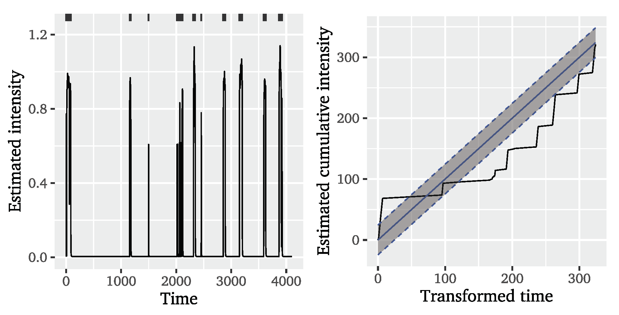
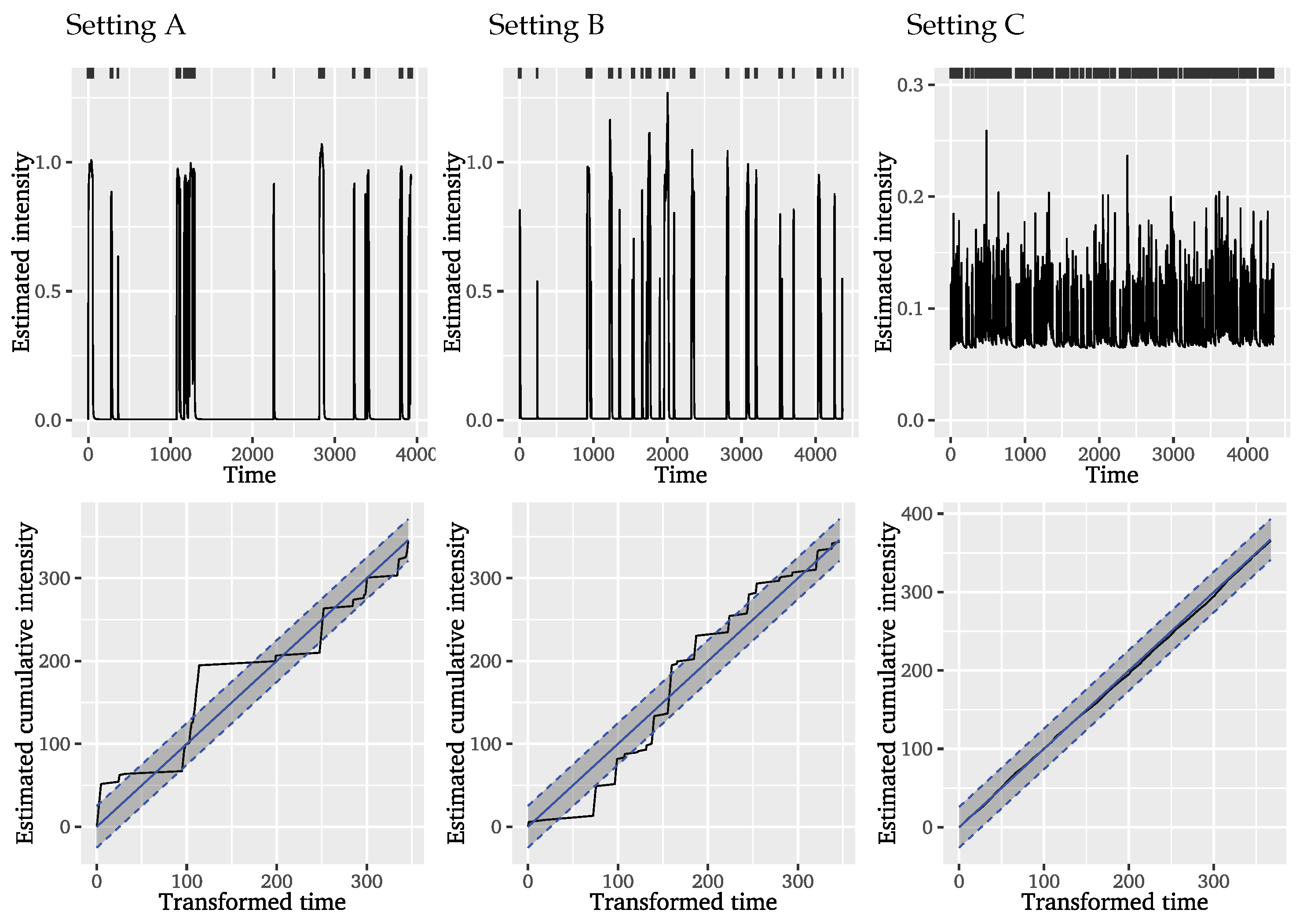
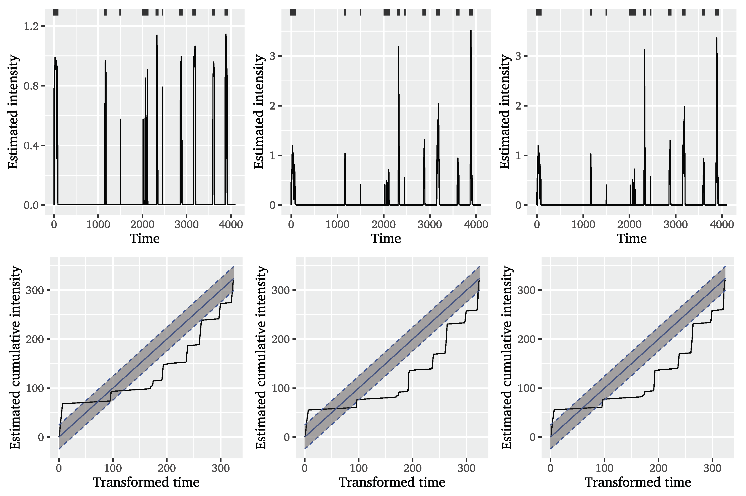
To evaluate the fit of the considered conditional POT models to the significant wave heights, we separately consider diagnostics for event time and mark modelling. For the evaluation of the fit to the event times, we look at two visual diagnostic tools: a plot of the estimated conditional intensity $\widehat{\lambda }$ and a plot of the cumulative intensity ${\Lambda }_{\mathcal{H}}\left(t_j\right)={\int }_0^{t_j}{\lambda }_{\mathcal{H}}\left(u\right)\mathrm{d}u$ against the time transformed based on the number of events. Figure 3 shows these diagnostics for the Hawkes-POT model with ETAS decay for the $7.9\%$ threshold, whereas the very similar looking plots for the exponential decay variant and both SEPOT models can be found in the Appendix A.1 in Figure A1.

The plotted estimated conditional intensities for the Hawkes-POT on the left of Figure 3 strongly differ from the results found for financial data by (e.g., [2,23]). The occurrence of an event causes the conditional intensity to instantly increase by an amount dependent on the mark size, which is followed by a rather sudden decline towards the estimated base rate $\widehat{\mu }$ after the last event of the cluster, likely due to the large estimated weight on the exponential dependence on past values. This is of course not realistic, but illustrates that the time span between observed events is so long that the dependencies captured by the conditional intensity fully disappear between clusters. Given the very small estimated ground intensities, it is actually very unlikely to see another event during the observation period based on these models, which contradicts the intuition that, the further away from the last event, the more likely it should be to see another cluster of events. The spiky appearance of the estimated conditional intensity results in a cumulative intensity resembling rather a step function than a line close to the bisecting one and therefore not lying within the $95\%$ confidence bands of the diagonal. From these visual diagnostics, we can conclude that of the conditional POT model variants are appropriate to model the event times in the significant wave height dataset. Their conditional intensities do not seem to sufficiently capture the dependencies in the data to explain the clustering behaviour.

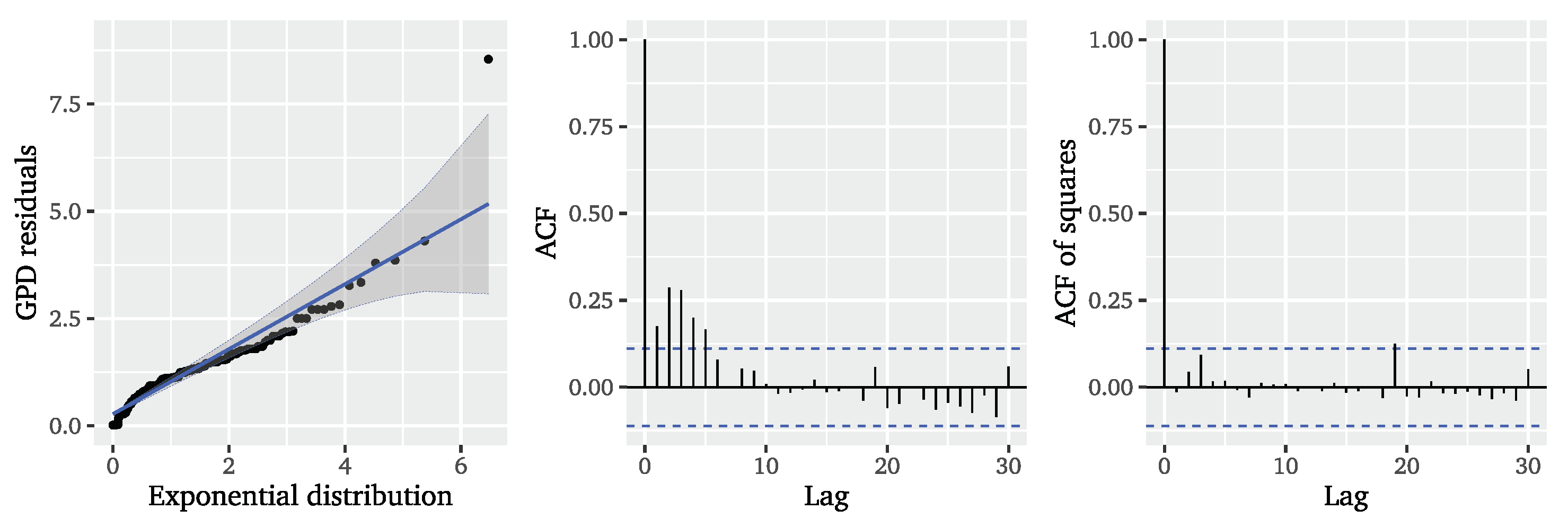
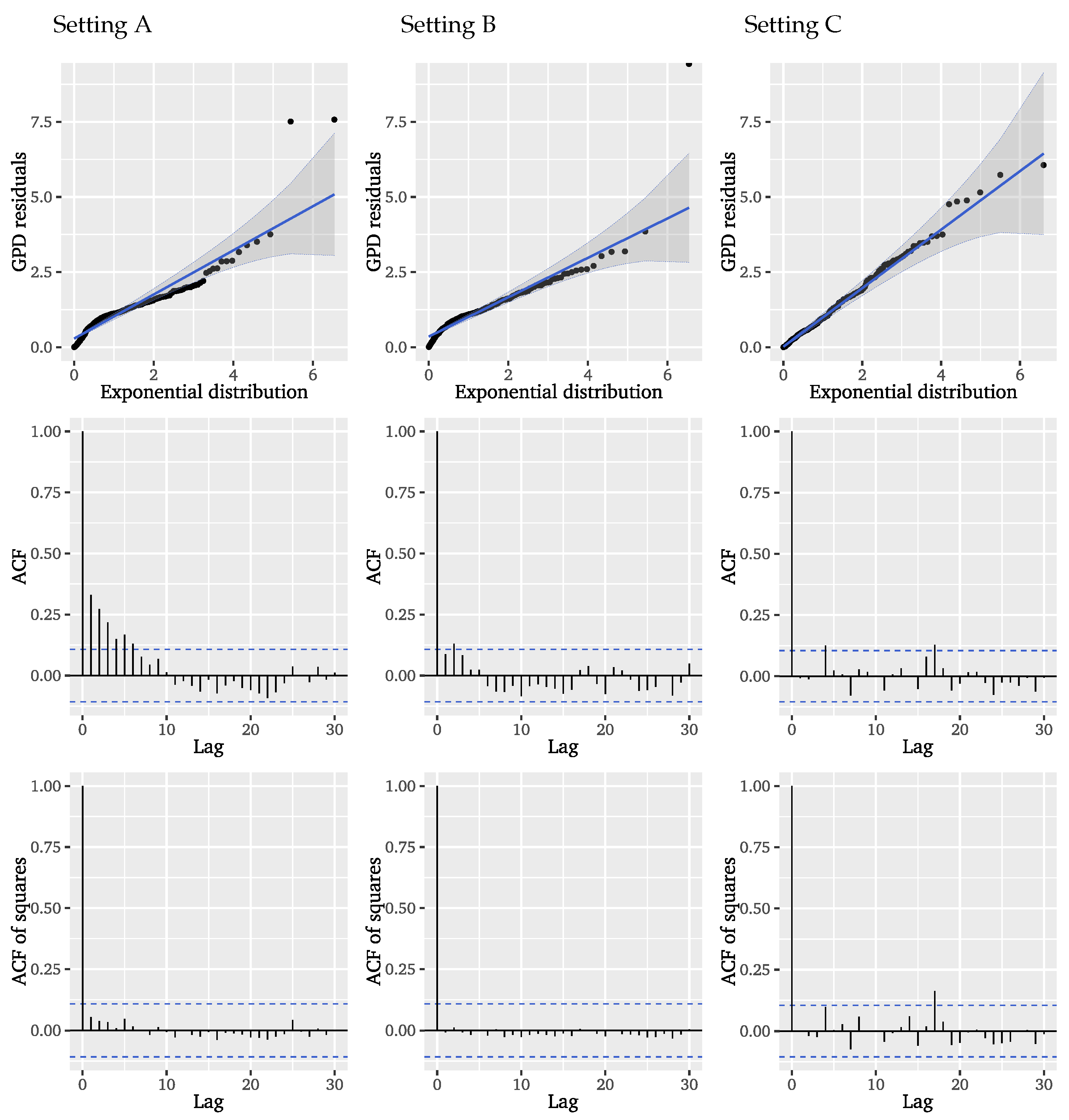
To evaluate the model fit for the event marks, we consider unit exponential QQ plots and plots of the ACF for the GPD residuals $R_j=\frac{1}{\widehat{\xi }}ln(1+\frac{\widehat{\xi }{y}_j}{\widehat{\beta }})$. Figure 4 depicts these visual diagnostics for the Hawkes-POT model with ETAS decay function. Similar results for the exponential decay and both SEPOT models can be found in the Appendix A.2 (Figure A2). The QQ plots reveal that in none of the considered setups the residuals are well-described by a unit exponential distribution as would be expected from a perfect fit. Although the Hawkes-POT model variants seem to give a more reasonable picture than the SEPOT model variants, the QQ plots confirm that there are still dependencies present that are not accounted for in the modelling of the mark sizes. This is validated by the ACF of the GPD residuals, which clearly depicts remaining autocorrelations for the first five lags indicating that the approach neglects dependencies. The squared residuals in contrast exhibit no systematic autocorrelations. From the residual diagnostics we can conclude that neither the considered Hawkes-POT nor SEPOT models can satisfactorily characterise the mark sizes in the significant wave height data. We may suspect that the long-range correlation found in the underlying series is responsible for depedencies that cannot be captured by the considered Hawkes-POT and SEPOT models. For this reason, we now turn to the next model that incorporates long-range dependence.

4.2. Results: Mittag–Leffler Distribution

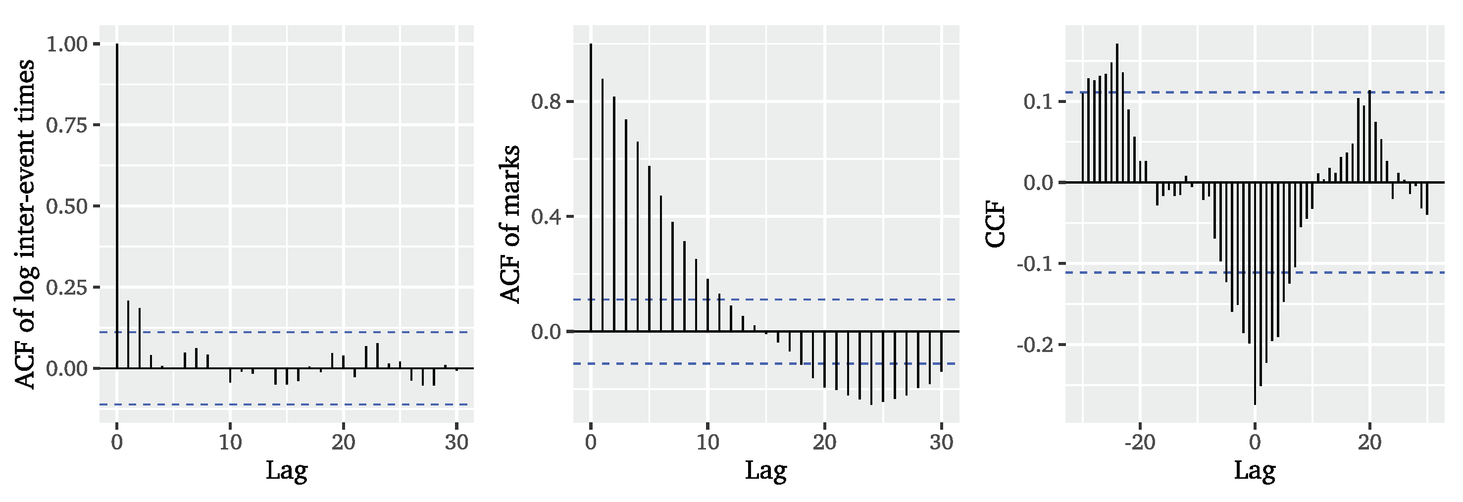
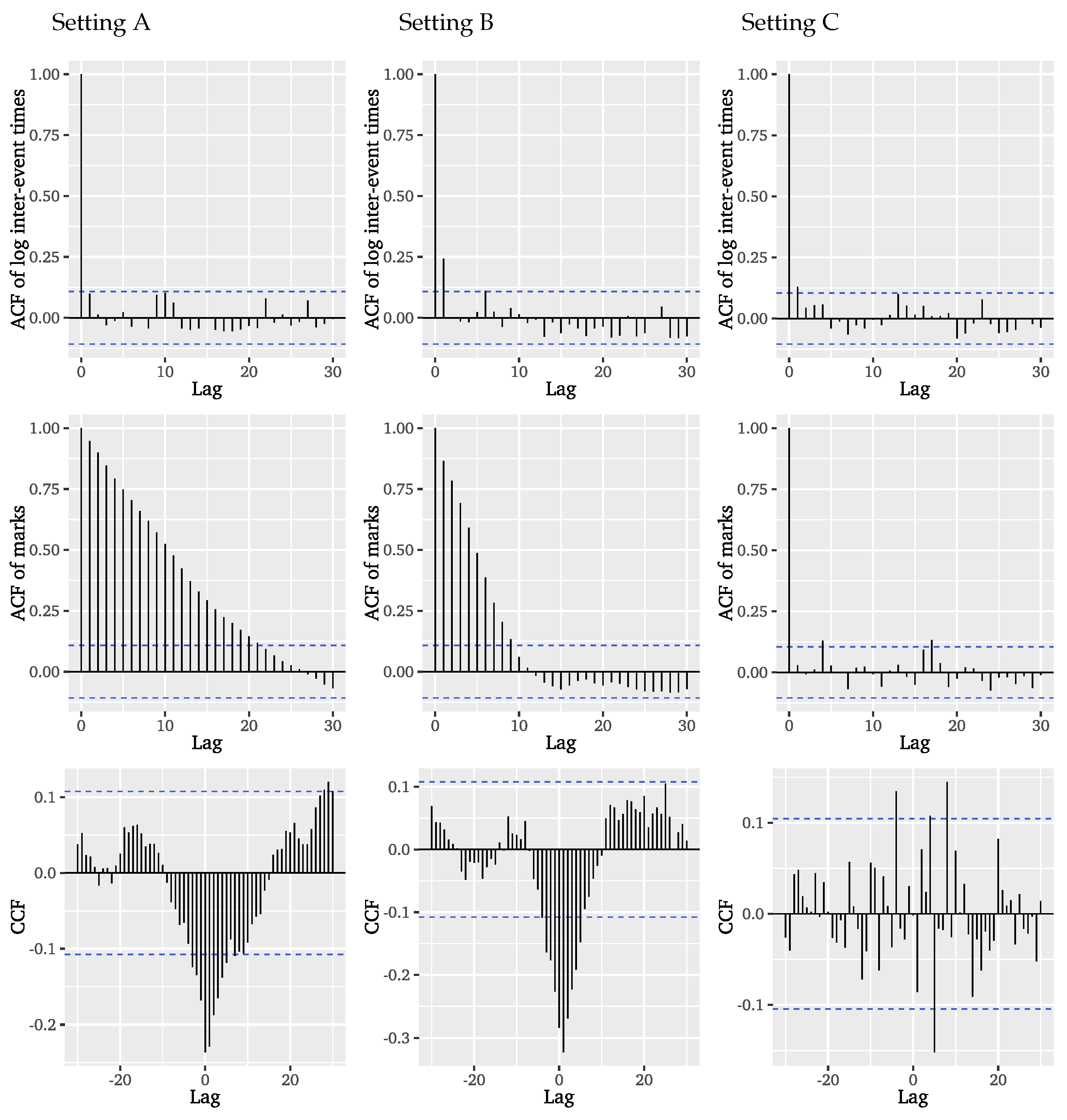
Following Hees et al. [43], we fit the Mittag–Leffler distribution to the inter-event times using the R packages MittagLeffleR [88] and CTRE [89]. We begin by checking the necessary assumptions. Firstly, the inter-event times and event marks are not supposed to exhibit any (inter-)dependencies. The ACF of the logarithmic inter-event times in Figure 5 reveals small autocorrelations for low lags, whereas the ACF of the event marks in Figure 5 shows strong autocorrelation for many lags.

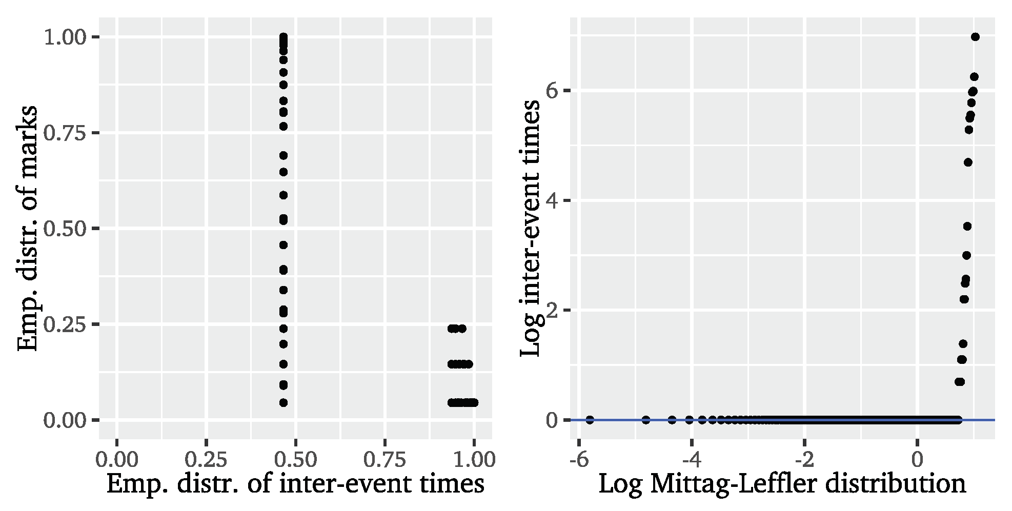
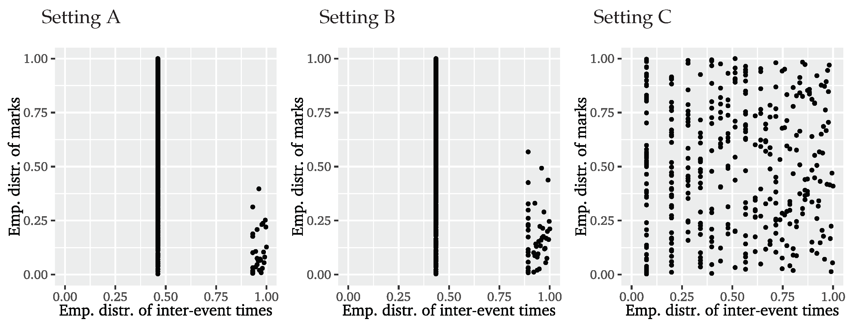
Considering the cross-correlation function (CCF) of inter-event times and event marks, we observe that the series are also cross-correlated, so that we clearly have to reject the independence assumption. The coupling of inter-event times and event marks is further confirmed by the empirical copula presented on the left of Figure 6. If both were uncoupled, the points would be evenly distributed over the $[0,1]\times [0,1]$ space. What we find instead is that the empirical copula is dominated by strong extremal clustering. The particular shape can be explained by events being mostly separated by a single time unit, so that there is an accumulation of points for this inter-event time combined with all possible values of event marks. After a long inter-event time, i.e., a long period without an event, we rather record smaller event marks, indicating that event clusters usually start with smaller marks which then magnify for the successive events.

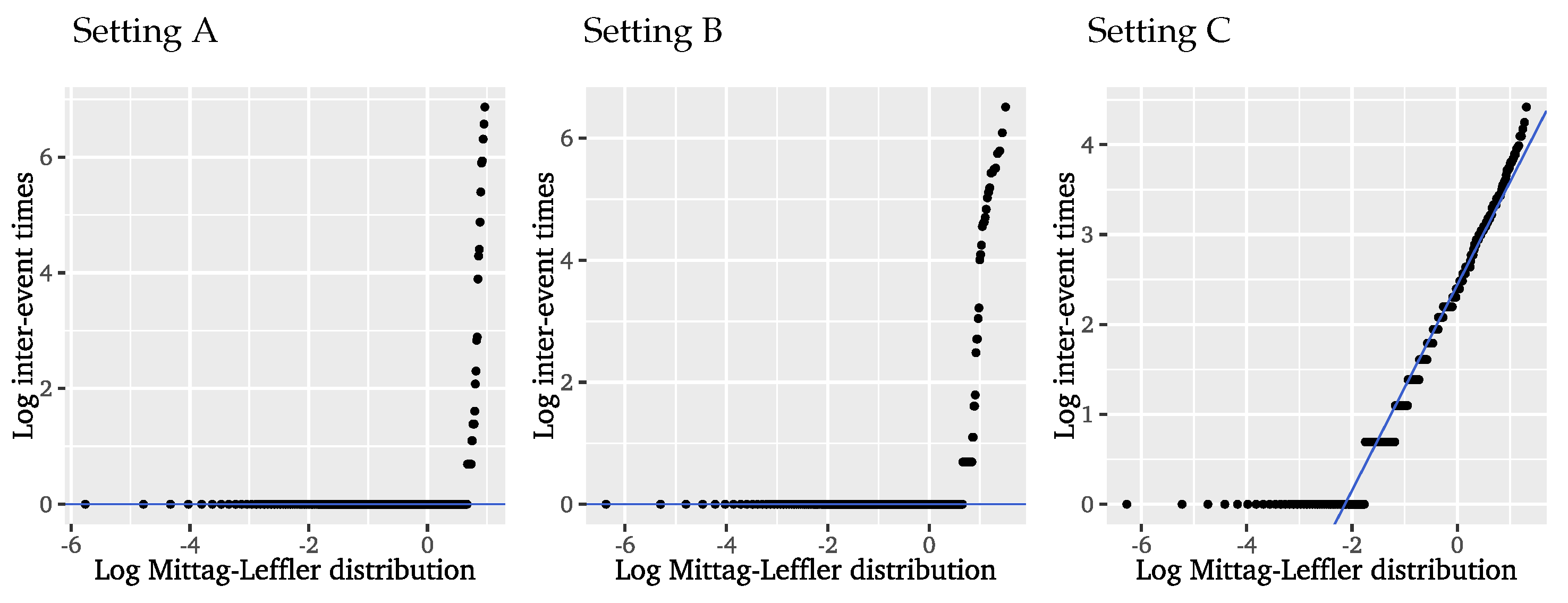
According to Hees et al. [43], the suitability of the Mittag–Leffler distribution can be verified using a logarithmic Mittag–Leffler QQ plot for the logarithmic inter-event times, displayed on the right of Figure 6. The tail parameter is determined via log-moment estimation yielding $\widehat{\beta }=1.1055$ with a $95\%$ confidence interval of $[1.0586;1.1524]$, which again strongly contradicts the model assumptions, while the scale is set to 1 for this diagnostic. It is obvious that the Mittag–Leffler distribution does not fit the inter-event times of the significant wave heights. Again, it appears that we have too much probability mass concentrated on lower, or more precisely, unit inter-event times, indicating that the present extremal clustering is too strong to be captured with this approach. Representing the long gaps between clusters, we further find a few inter-event times that are too large to appear under a Mittag–Leffler distribution. Given these results, we can conclude that the Mittag–Leffler distribution does not provide a better fit to the inter-event times of the significant wave heights than the exponential distribution arising in the limit of iid data. Even though this approach incorporates long-range dependence, it does only account for it in the event times and disregards any local, short-range dependencies affecting the distribution of event and inter-event times.

Although the assumptions are obviously violated, we include the parameter estimates of the Mittag–Leffler distribution for the significant wave height data for completeness. The stability plots for the tail and re-scaled scale are presented in Figure 7 and do not give clear stable regions for the parameter estimates. For the tail parameter, the only rather stable region we can identify is around the estimate $\widehat{\beta }=1.12$, which is consistent with the previous estimation and again clearly violates the model assumptions. Additionally, the scale parameter is dependent on the number of events, indicating that the model is not suitable for the significant wave height dataset.

To date, neither the applied conditional POT methods nor the fitted Mittag–Leffler distribution satisfactorily explain the extremal clustering in the significant wave height data. Either the models fail to account for the long-range dependence in the mark sizes inherited from the dependence structure of the underlying observations, or the short-range dependencies between the event times are disregarded. Therefore, we continue with applying the two-step ARFIMA-POT approach which aims at capturing the full dependence structure of the underlying observations, in order to avoid the need for explicit modelling of inherited properties in the event times and mark sizes all together.

4.3. Results: Two-Step ARFIMA-POT Approach

In the first stage of the two-step ARFIMA-POT approach, we seek to identify and fit the ARFIMA$(p,d,q)$ model that is most suitable for describing the significant wave heights. Using the R package arfima [90], we systematically estimate the model parameters including d for various combinations of p and q orders and find the ARFIMA model with $p=4$ and $q=4$ to minimise both AIC and BIC.

Table 2. Estimation results of the ARFIMA$(p,d,q)$ model. Standard errors in parentheses.

${\widehat{\mathit{\phi }}}_1$	${\widehat{\mathit{\phi }}}_2$	${\widehat{\mathit{\phi }}}_3$	${\widehat{\mathit{\phi }}}_4$	$\widehat{\mathit{d}}$	${\widehat{\mathit{\theta }}}_1$	${\widehat{\mathit{\theta }}}_2$	${\widehat{\mathit{\theta }}}_3$	${\widehat{\mathit{\theta }}}_4$
1.1787	−0.3177	0.8687	−0.7375	0.1398	0.3660	−0.2593	0.7555	−0.1270
(0.0874)	(0.1591)	(0.1126)	(0.0528)	(0.1634)	(0.2104)	(0.1041)	(0.1138)	(0.0905)
$lnL$	$AIC$	$BIC$
10,354.4	−20,686.8	−20,616.6

reports the parameter estimates for the selected ARFIMA model. The corresponding fractional difference parameter is estimated as $0.1398$ indicating the presence of mild long-range dependence.

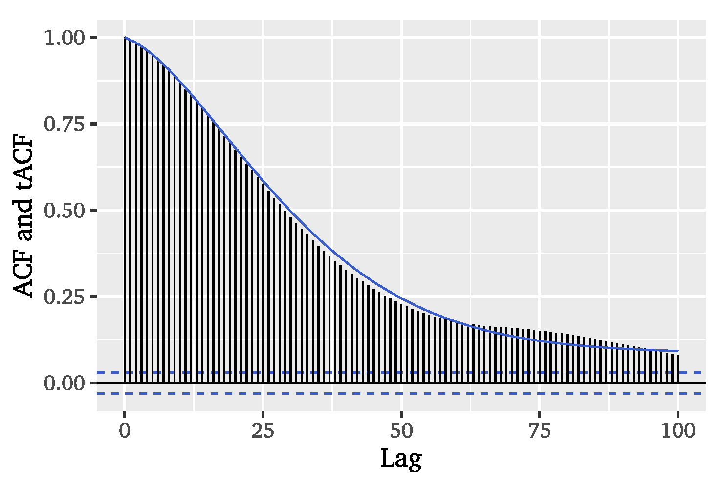
Comparing the theoretical ACF of the chosen ARFIMA model to the empirical ACF of the dataset in Figure 8, we can conclude that the selected model specification satisfactorily captures the autocorrelation structure of the significant wave heights.

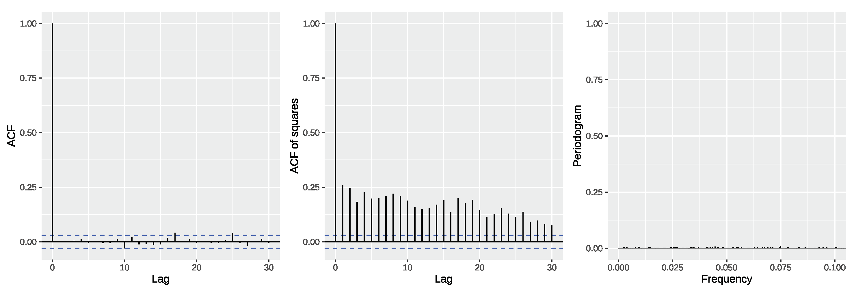
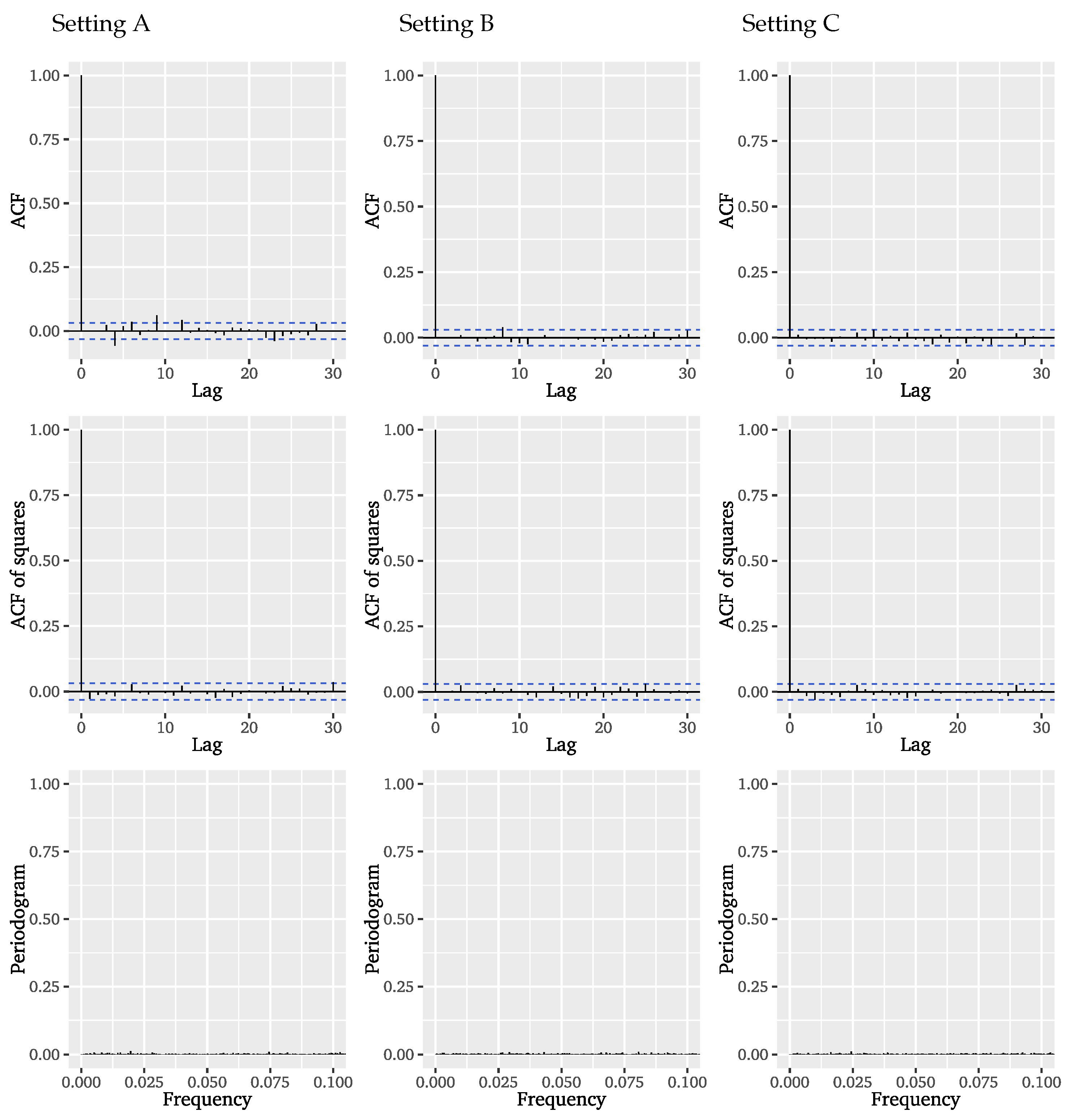
Further, Figure 9 provides visual diagnostics for the ARFIMA model residuals in the form of plotted ACFs of residuals and squared residuals as well the periodogram of the residuals. These diagnostic suggest that, apart from some variance clustering, there are no dependencies left in the residuals. Since we deliberately refrained from modelling the conditional variance of the significant wave heights in order to solely find an explicit representation of the dependence structure of the underlying series, the residual diagnostics confirm suitability of the classical POT model for the ARFIMA model residuals. An additional Ljung-Box test for the smallest possible lag choice, which results from the model orders and corresponds to 9 lags in this case (see [91]), does not reject the null hypothesis of no autocorrelation in the ARFIMA residuals for the considered lags on a $10\%$ level (p-value: 0.1642).

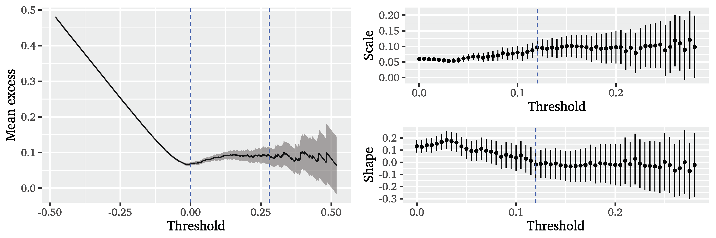
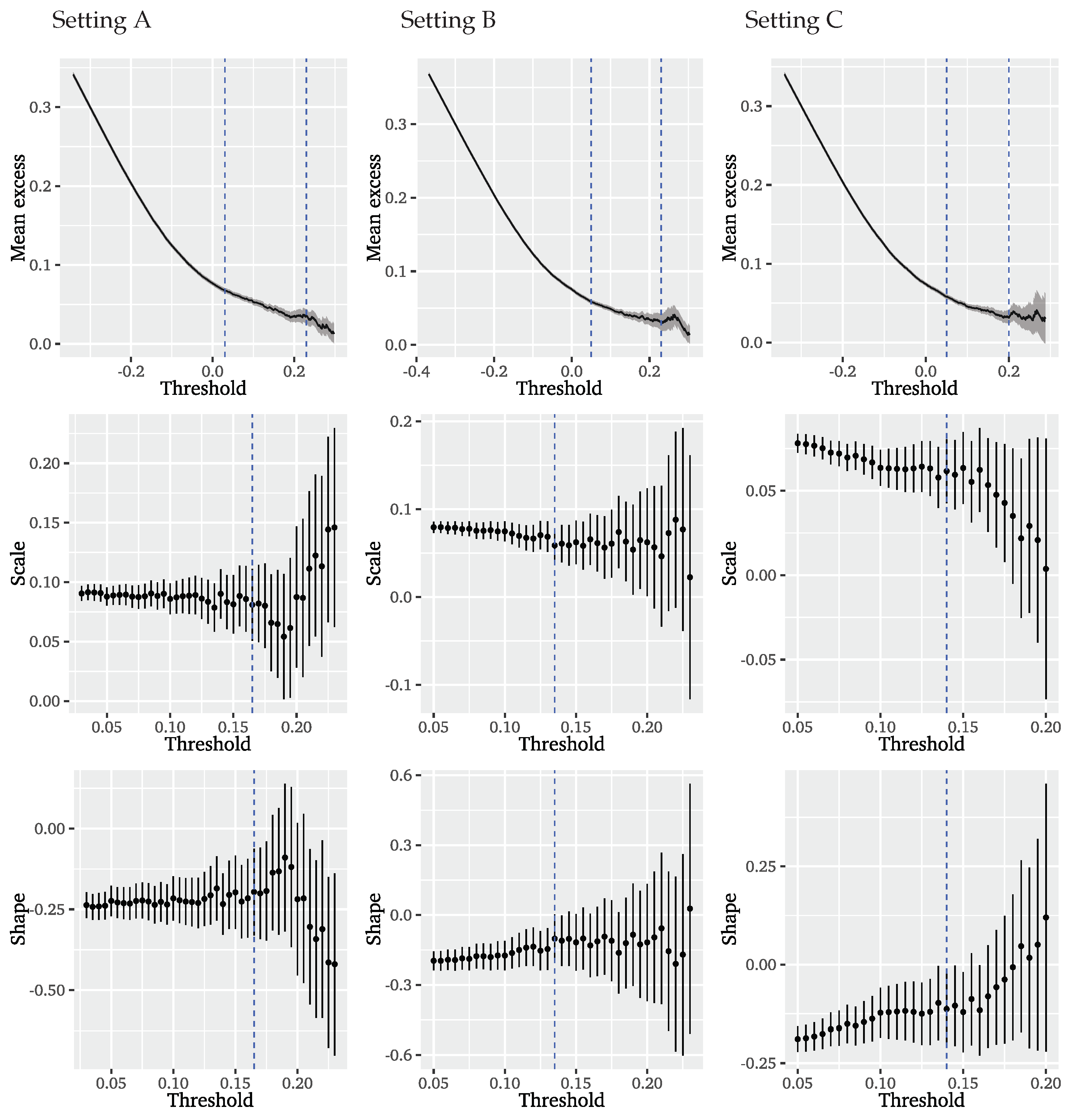
In the second stage of the ARFIMA-POT approach, we apply the classical POT method to the ARFIMA residuals using the R packages POT [92] and extRemes [93]. The threshold is chosen from the mean residual life plot and GPD parameter stability plots given in Figure 10. The mean excess plot shows a course linear in u from 0 to $0.12$ and is rather constant between $0.12$ and $0.28$. Choosing a higher threshold is not sensible due to the erratic course of the mean excess and too few remaining observations. The GPD parameter stability plots suggest a long stable region for both GPD parameter estimates following a threshold of $u=0.12$ that corresponds to $7.3\%$ of data and matches the threshold from the mean residual life plot. Thus, we base the second step of the ARFIMA-POT approach on a threshold corresponding to $7.3\%$ of data.

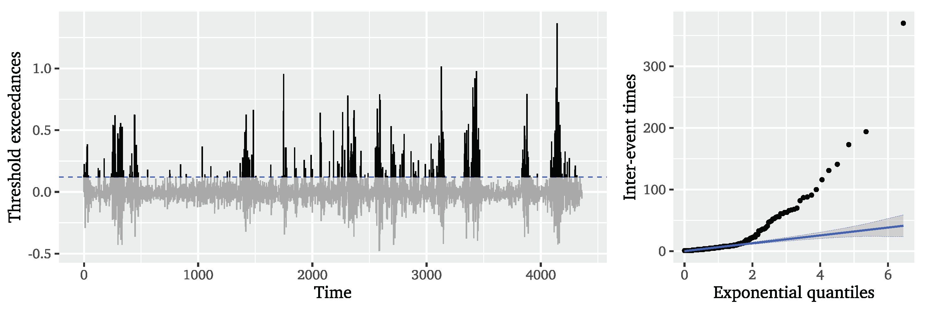
Based on the ARFIMA residuals, Figure 11 displays the exceedances of the selected threshold. In line with the autocorrelations found in the ACF of the squared ARFIMA residuals (cf. Figure 9), the extreme events still appear to be slightly clustered, but the long gaps without clusters that governed the original significant wave height series are no longer as distinct. The QQ plot of the inter-event times on the right of Figure 11 still depicts the tails of the inter-event times as lying outside the confidence bands of the exponential distribution, but this is much closer to the exponential distribution than what was observable for the original time series (cf. Figure 1). We can note that the two-step ARFIMA-POT approach improves the predictability of event times over the original series, but the dynamics of the significant wave height series affecting the distribution of event times are not captured in their entirety.

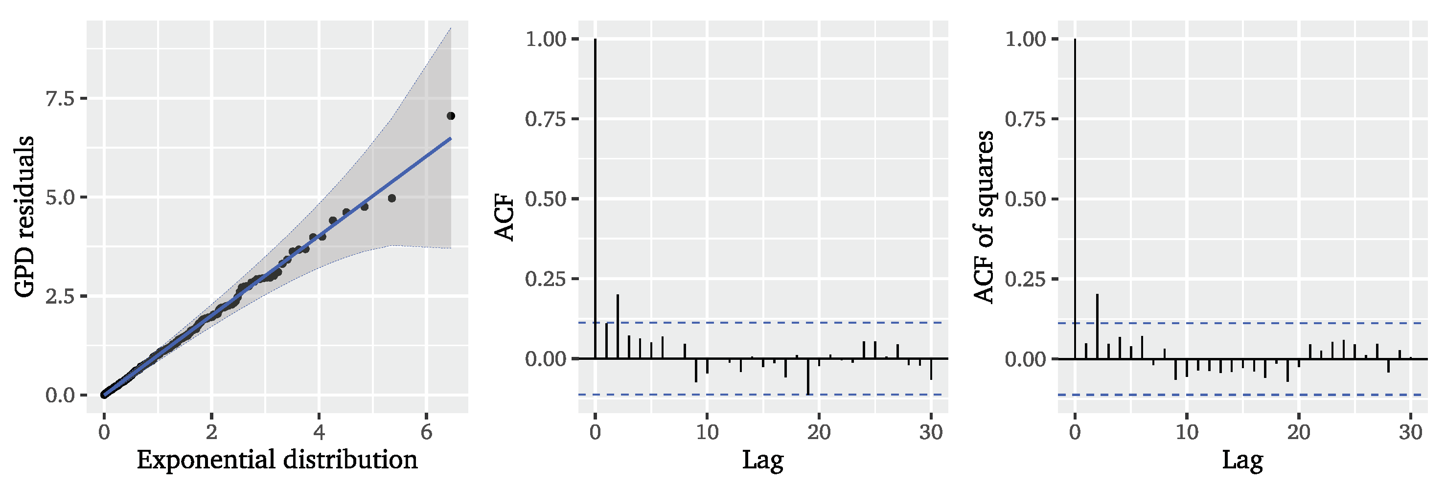
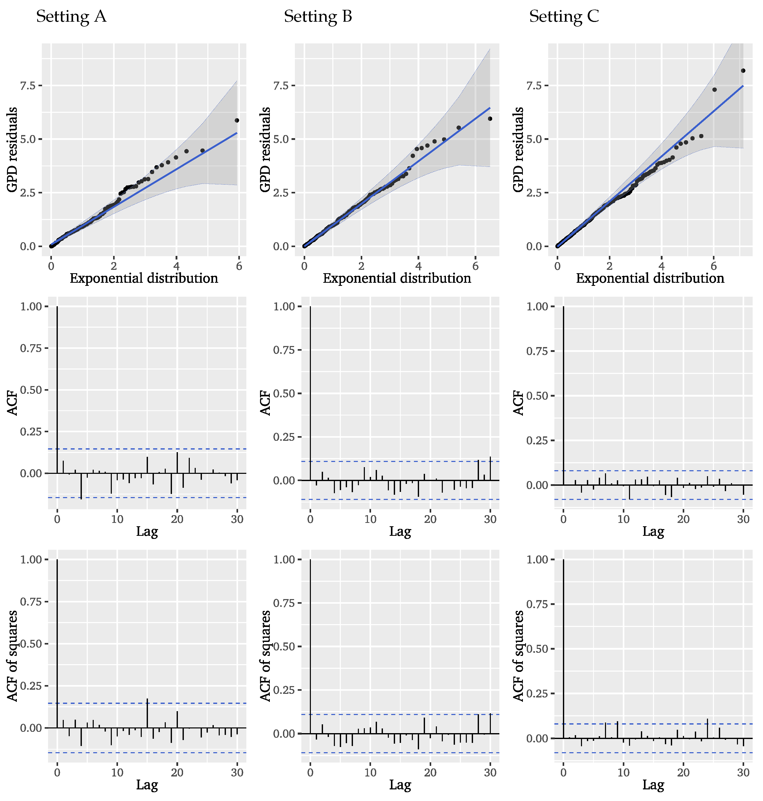
We fit a GPD to the ARFIMA residuals via maximum likelihood estimation and obtain the estimates $\widehat{\beta }=0.0944$$\left(0.0074\right)$ and $\widehat{\xi }=-0.0189$$\left(0.0554\right)$ for scale and shape parameters, respectively. Similar to the results for the conditional POT approaches, the estimated shape parameter is negative, indicating a finite tail of the distribution of ARFIMA residuals and a concentration of probability mass on the smaller mark sizes. Based on the estimated GPD residuals, Figure 12 provides visual diagnostics. The QQ plot illustrates that the GPD residuals are following a unit exponential distribution very closely. Compared with the results for the Hawkes-POT in Figure 4, we find a clearly improved model fit. Considering the ACF of the GPD residuals and squared residuals, we observe that, apart from lag 2, there is no autocorrelation left, indicating that the two-step ARFIMA-POT approach satisfactorily models the dependencies in the underlying significant wave height series which may affect the distribution of the mark sizes.

In summary, the two-step ARFIMA-POT approach improves upon the considered conditional POT approaches in terms of model fit for the mark sizes, and upon the fit of the Mittag–Leffler distribution for the inter-event times. Clearly, the two-step method is an imperfect solution to modelling significant wave heights, but we show that incorporating both short- and long-range dependencies in a parametric approach can be a more successful pathway than focusing on short- or long-term dynamics alone. To review these conclusions, we systematically break down the effects of short- and long-range dependence on the model fits in the following section.

5. Simulation Study

In Section 4, we argued that the combination of short- and long-range dependence is pivotal to the unsatisfactory fits of the conditional POT models and the Mittag–Leffler distribution to the significant wave height data. In order to verify these results and the appropriateness of the two-step ARFIMA-POT approach, we conduct a simulation study. The overall objective is to rule out the possibility of spurious results. Therefore, we aim at demonstrating that the observations for significant wave heights and our corresponding conclusions are of a systematic nature and can be reproduced.

The two-step ARFIMA-POT approach is based on the assumption that dependencies in the underlying time series are well-characterised by an ARFIMA model. Therefore, we consider a base setting in which we simulate data from an ARFIMA model with a specification that is similar to the one estimated for the significant wave height dataset in Section 4.3, i.e., we simulate from an ARFIMA$(4,0.1398,4)$ with parameters given in Table 2 (setting A). Further, we consider two additional settings in which either the ARMA orders p and q are set to zero (setting B) or the fractional difference parameter d (setting C). Thus, the settings B and C correspond to data in which the short- or long-range correlations are eliminated, respectively. Analogous to the size of the significant wave height dataset, we simulate 4367 data points for each setting and then apply all considered methods to the resulting datasets to evaluate the model fits.

5.1. Simulation Results: Conditional POT Models

We begin by examining the estimation results for the conditional POT models based on a threshold of $7.9\%$ in the considered settings A, B, and C, which are presented in

Table 3. Estimation results of the Hawkes-POT and SEPOT model for the simulated settings A, B and C. Italic numbers represent bounds of the estimation region.

Model	Parameter Estimates
	${\widehat{\mu }}_0$	${\widehat{\mu }}_1$	$\widehat{\gamma }$	$\widehat{\delta }$	$\widehat{\rho }$	$\widehat{a}$	$\widehat{b}$	$\widehat{\xi }$	$lnL$
Setting A
Hawkes-POT (ETAS)	0.0032	1.5319	0.4026	0.1131	1.6573	−1.4181	1.7329	−0.7442	−284.34
Hawkes-POT (exp.)	0.0039	1.2625	0.8652	0.1151		−1.4181	1.7329	−0.7442	−287.29
Setting B
Hawkes-POT (ETAS)	0.0061	25.0000	1.6975	0.5433	2.8912	−2.0768	3.0946	−0.4550	−244.51
Hawkes-POT (exp.)	0.0063	1.1710	0.8903	0.5201		−2.0768	3.0946	−0.4550	−243.66
Setting C
Hawkes-POT (ETAS)	0.0631	0.2191	1.3713	4.2724	0.6793	−3.0999	0.8702	−0.1139	−459.20
Hawkes-POT (exp.)	0.0686	0.0641	0.3523	4.2263		−3.0999	0.8702	−0.1139	−459.80
	${\widehat{\mu }}_0$	${\widehat{\mu }}_1$	$\widehat{\gamma }$	$\widehat{\delta }$	$\widehat{\rho }$	${\widehat{\beta }}_0$	${\widehat{\beta }}_1$	$\widehat{\xi }$	$lnL$
Setting A
SEPOT (ETAS)	0.0179	0.0895	0.0769	0.9464	0.4790	0.4468	0.4588	−2.0036	−746.99
SEPOT (exp.)	0.0042	0.9184	1.0045	1.3580		0.1622	0.3504	−0.6942	−337.26
Setting B
SEPOT (ETAS)	0.0062	0.7576	0.2879	2.0363	1.6669	0.1032	0.1784	−0.5555	−256.88
SEPOT (exp.)	0.0065	0.8785	0.9632	2.0715		0.1014	0.2057	−0.5494	−254.48
Setting C
SEPOT (ETAS)	0.0677	0.2445	0.0441	0.7526	0.4411	0.4411	0.0442	−2.1149	−959.58
SEPOT (exp.)	0.0688	0.0629	0.3583	4.8278		0.0461	0.0015	−0.1118	−460.01

. The parameter estimates in the settings A and B are mostly found to be in a similar range as reported for the significant wave height dataset in Table 1. For setting C, however, we observe quite different results, i.e., for the setting that only includes long-range dependence: for both Hawkes- and SEPOT model variants, the base rate of the conditional intensity of the ground process ${\widehat{\mu }}_0$ has increased approximately tenfold, which already suggests a more homogeneous behaviour of the conditional intensity. The estimates for the factor ${\widehat{\mu }}_1$ are generally smaller implying less pronounced reactions on previous events, but this effect is potentially balanced out for the mark sizes by the mostly larger estimates $\widehat{\delta }$. With respect to the ETAS decay model variants, we find a smaller estimate $\widehat{\rho }$ in setting C, resulting in a higher impact of distant events. A similar effect is observed for the exponential decay models through a smaller estimate $\widehat{\gamma }$.

For the Hawkes-POT variants, we find estimates for $\widehat{b}$ which are noticeably smaller, indicating that the scale parameter of the conditional GPD is less dependent on the previous mark size. This observation is even more apparent for the parameter ${\widehat{\beta }}_1$ in case of the SEPOT model variants where the estimates are close to zero, indicating a rather constant GPD scale parameter. Thus, we can conclude that the strongly time-varying nature of the scale parameter of the conditional GPD in settings A and B is rather the result of short-term, ARMA-type correlations in the data. Considering the estimation results, the dataset in setting C appears to have properties that can be handled more realistically by the conditional POT approaches than the settings A and B.

To verify this presumption, we provide various visual diagnostics. As an example, we present the diagnostics for the Hawkes-POT with ETAS decay function, as the results for the other conditional POT variants were found to be very similar. Figure 13 displays the estimated conditional intensities and the cumulative conditional intensities for all three simulation settings. The results for setting A show a similar pattern as was observed for the significant wave heights in Figure 3, indicating that the conditional POT models are not well-suited for ARFIMA-type time series. Setting B improves upon the results for setting A, presumably because the events appear to exhibit less pronounced extremal clustering, as can be seen from slightly more equally distributed event ticks. The simulated fractional white noise in setting C, i.e., the ARFIMA$(0,0.1398,0)$, follows completely different dynamics with only slight extremal clustering. Fractional integration only seems to intensify the particular clustering behaviour when short-range correlations are already present, as visible when comparing settings A and B, while it has little effect when added to a white noise sequence using a fractional difference parameter d that is this low. In consequence, the conditional POT model seems to be an appropriate fit for the data of setting C, leading to a well-shaped estimated conditional intensity and a cumulative intensity that evenly spreads across events.

The residual diagnostics in Figure 14, consisting of ACFs for GPD residuals and squared residuals as well as unit exponential QQ plots for the three simulation settings, confirm these findings. In the GPD residuals of the Hawkes-POT in setting A there is still a large amount of autocorrelation left, which is similar, albeit more pronounced than what was observed for the significant wave height dataset in Figure 4. This also leads to the GPD residuals being far from unit exponentially distributed. The diagnostics improve when switching to setting B, so a situation with short-range dependent, ARMA-type data. In setting C, the conditional POT appears to capture all dependencies in the data, so that assuming a unit exponential distribution for the GPD residuals seems reasonable, which strengthens our previous findings.

In summary, the simulation study for the conditional POT models shows that the combination of short- and long-range dependence in the data leads to pronounced extremal clustering. We can conclude that the more extreme the clustering behaviour in the extreme events gets, the less appropriate this type of model is. The long-range dependence itself does not appear to be causal for the unsatisfactory model fit, but rather the impact that the long-range correlation has on the extremes in data that is already governed by short-term dependencies. Therefore, we can note that the combination of short- and long-range dynamics leads to a deterioration in the model fit for conditional POT approaches, confirming the presumptions from Section 4.1.

5.2. Simulation Results: Mittag–Leffler Distribution

Next, we consider fitting the Mittag–Leffler distribution to the inter-event times for the simulated settings A, B and C. Figure 15 provides the ACFs of logarithmic inter-event times and event marks as well as their CCF for all simulation settings. For setting C, we find no systematic correlations, implying that the Mittag–Leffler distribution may be suitable to a pure long-range dependence setting. However, it is obvious from setting B that the autocorrelation in the event marks and the cross-correlation between event times and event marks are induced by the short-range, ARMA-type dependencies. Comparing the results from settings A and B, we can further state that when combining the ARMA-dependencies with a fractionally integrated component, the observed correlations appear even more pronounced. Similar conclusions can be drawn from the empirical copulas for the inter-event times and event marks, depicted in the Appendix A.2 in Figure A3.

Figure 16 presents the logarithmic Mittag–Leffler QQ plots of the logarithmic inter-event times for all settings. Again, it is apparent that in settings A and B the Mittag–Leffler distribution does not seem to be appropriate for the inter-event times. For setting C, we note a substantially improved fit, but still observe distinct deviations for lower quantiles.

The parameter stability plots for the tail and re-scaled scale estimates of the Mittag–Leffler distribution are given in Figure 17 for all simulation settings. Clearly, the presence of short-ranged ARMA dependencies in settings A and B leads to an absence of areas of stability for tail and especially re-scaled scale estimates. In setting C, however, it is easy to identify stability regions, implying that the Mittag–Leffler distribution may be well-suited for a situation in which the underlying data is only governed by long-range dependence.

From these simulation results, we can conclude that modelling the inter-event times by means of a Mittag–Leffler distribution is not appropriate when the underlying time series not only exhibits long-range dependence, but also short-term correlations. This confirms the findings from the application of the Mittag–Leffler distribution to significant wave heights in Section 4, which posed a situation in which the dependence structure of the data can only be characterised by a combination of short- and long-range dynamics.

5.3. Simulation Results: Two-Step ARFIMA-POT Approach

Lastly, we continue the simulation study by investigating whether the two-step ARFIMA-POT approach is suitable for ARFIMA-type dependencies in the time series, even when considering only either ARMA components or fractional integration. For this, we make use of the same settings A, B, and C as before and apply the same two-step ARFIMA-POT procedure as described in detail with the application to significant wave heights in Section 4.3: we first estimate the ARFIMA model with the AR and MA orders being selected according to the BIC, and calculate the ARFIMA residuals, to which we then apply the classical POT model. The corresponding estimation results for all settings are stated in

Table A1. Estimation results of the ARFIMA$(p,d,q)$ model for the simulated settings A, B, and C. Standard errors in parentheses.

	${\widehat{\mathit{\phi }}}_1$	${\widehat{\mathit{\phi }}}_2$	${\widehat{\mathit{\phi }}}_3$	${\widehat{\mathit{\phi }}}_4$	$\widehat{\mathit{d}}$	${\widehat{\mathit{\theta }}}_1$	${\widehat{\mathit{\theta }}}_2$	${\widehat{\mathit{\theta }}}_3$	${\widehat{\mathit{\theta }}}_4$
Setting A	0.7272	0.2389			0.2577
	(0.0255)	(0.0219)			(0.0232)
Setting B	1.1527	−0.2355	0.8372	−0.7609	0.0842	0.3924	−0.1814	0.7920	−0.1216
	(0.0495)	(0.0912)	(0.0936)	(0.0487)	(0.0786)	(0.1025)	(0.0640)	(0.0732)	(0.0607)
Setting C					0.1549
					(0.0122)
	$lnL$	$AIC$	$BIC$
Setting A	9228.0	−18445.9	−18414.5
Setting B	10355.7	−20689.4	−20619.3
Setting C	10353.8	−20701.7	−20682.5

in Appendix A.2.

Similar to the results for the significant wave height data, the ARFIMA residuals do not exhibit any remaining autocorrelation regardless of the considered setting (see Figure A4 in Appendix A.2). Additional Ljung-Box tests for the smallest possible lags in each setting support this. The null hypothesis of no autocorrelation cannot be rejected on a $10\%$ level for settings A and C (p-values: 0.1453 and 0.4606, respectively). Only for setting B, the null hypothesis can be rejected on a $1\%$ level (p-value: 0.0017). This, however, is neither too surprising nor worrisome since the setting forces the ARMA parameters to zero implying that any remaining random variations can hardly be captured systematically. The thresholds for the three settings were again determined using mean residual life plots and corresponding parameter stability plots, which can be found in Appendix A.2 in Figure A5 for reference. The selected thresholds are $u_A=0.165$ m ($4.78\%$), $u_B=0.135$ m ($7.70\%$), and $u_C=0.1$ m ($14.36\%)$ for the settings A, B, and C, respectively. For setting C, it is worth mentioning that the small fractional component induces a weaker dependence structure compared to settings A and B, resulting in the GPD being appropriate for a lower threshold and therefore larger tail of the residual distribution. For all three settings, the estimation results of the second stage of the ARFIMA-POT method, i.e., fitting of a GPD to the ARFIMA residuals, can be found in

Table A2. Estimation results of the GPD fit to the ARFIMA$(p,d,q)$ residuals for the simulated settings A, B, and C. Standard errors in parentheses.

	$\widehat{\mathit{\beta }}$	$\widehat{\mathit{\xi }}$
Setting A	0.0486 (0.0048)	−0.1962 (0.0684)
Setting B	0.0451 (0.0034)	−0.1014 (0.0528)
Setting C	0.0514 (0.0026)	−0.1224 (0.0324)

in Appendix A.2.

Figure 18 provides visual diagnostics for the GPD residuals in the form of unit exponential QQ plots and ACFs of residuals and squared residuals. The GPD residuals of the two-step ARFIMA-POT approach show a noticeably better fit than the GPD residuals of the conditional POT approaches in Figure 14. In all three settings, there is no systematic autocorrelation left, and the distribution of the GPD residuals comes close to a unit exponential distribution. Thus, the two-step ARFIMA-POT approach works equally well regardless of whether we only find short-term ARMA correlations, fractional integration or both types of dependencies in the underlying dataset.

This simulation study clearly highlighted that the two-step ARFIMA-POT approach is advantageous in situations in which it is unclear what type of dependencies are present in the data. As opposed to the conditional POT models and the Mittag–Leffler distribution, the approach still provides a useful characterisation of the extremal behaviour in cases in which both short- and long-range correlations govern the underlying time series, as found for the significant wave height dataset.

6. Conclusions

We considered a setting in which short- and long-range dependencies in the underlying time series of significant wave heights lead to pronounced clustering behaviour of high threshold exceedances. We reviewed commonly used conditional POT models which parametrically model the short-term dynamics underlying the extremal clustering, as well as the Mittag–Leffler distribution for inter-event times incorporating long-range correlations in the implied event times. For both approaches, we found that long- or short-term dependencies were neglected, respectively, resulting in unsatisfactory model fits to the significant wave height data. In a simulation study, we confirmed that the combination of short- and long-range correlations is pivotal to this observation.

To prevent event times and mark sizes from inheriting properties of the dependence structure of the underlying series that would have to be modelled explicitly, we suggested the two-step ARFIMA-POT approach. This two-step approach first fits an ARFIMA model to the significant wave heights capturing the short- and long-term correlations of the observations, and then applies a classical POT model to the residuals. We found that the two-step ARFIMA-POT approach provides significant improvements in terms of model fit for the significant wave heights. Additionally, a simulation study confirmed that the two-step ARFIMA-POT approach enables a sensible characterisation of extreme events in case of ARFIMA-type dependencies in the time series, even when considering only either ARMA components or fractional integration.

Our results illustrate the need for new methods filling the gap at the intersection of modelling local clustering behaviour and long-range dependence. Clearly, our solution to this issue is a pragmatic one, but it provides a strategy that is easily applicable and interpretable by practitioners. However, future work should address this challenge by developing models with a sound mathematical underpinning, possibly combining existing approaches to focus on short-term dynamics with long-range dependent components and vice versa.

References

1. Ferreira, A.; de Haan, L. On the block maxima method in extreme value theory: PWM estimators. Ann. Stat. 2015, 43, 276–298. [Google Scholar] [CrossRef] [Green Version]
2. Chavez-Demoulin, V.; Davison, A.C.; McNeil, A.J. Estimating value-at-risk: A point process approach. Quant. Financ. 2005, 5, 227–234. [Google Scholar] [CrossRef]
3. Herrera, R.; Schipp, B. Statistics of extreme events in risk management: The impact of the subprime and global financial crisis on the German stock market. N. Am. J. Econ. Financ. 2014, 29, 218–238. [Google Scholar] [CrossRef]
4. Lee, D.; Li, W.K.; Wong, T.S.T. Modeling insurance claims via a mixture exponential model combined with peaks-over-threshold approach. Insur. Math. Econ. 2012, 51, 538–550. [Google Scholar] [CrossRef]
5. Bernardara, P.; Andreewsky, M.; Benoit, M. Application of regional frequency analysis to the estimation of extreme storm surges. J. Geophys. Res. 2011, 116, C2. [Google Scholar] [CrossRef]
6. Dissanayake, P.; Brown, J.; Sibbertsen, P.; Winter, C. Using a two-step framework for the investigation of storm impacted beach/dune erosion. Coast. Eng. 2021, 168, 103939. [Google Scholar] [CrossRef]
7. Méndez, F.J.; Menéndez, M.; Luceño, A.; Losada, I.J. Estimation of the long-term variability of extreme significant wave height using a time-dependent Peak Over Threshold (POT) model. J. Geophys. Res. 2006, 111, C7. [Google Scholar] [CrossRef]
8. Cañellas, B.; Orfila, A.; Méndez, F.J.; Menéndez, M.; Gómez-Pujol, L.; Tintoré, J. Application of a POT Model to Estimate the Extreme Significant Wave Height Levels around the Balearic Sea (Western Mediterranean); Coastal Education and Research Foundation: Coconut Creek, FL, USA, 2007. [Google Scholar]
9. Davison, A.C.; Smith, R.L. Models for exceedances over high thresholds. J. R. Stat. Soc. Ser. B Methodol. 1990, 52, 393–425. [Google Scholar] [CrossRef]
10. Smith, R.L.; Weissman, I. Estimating the extremal index. J. R. Stat. Soc. Ser. B Methodol. 1994, 56, 515–528. [Google Scholar] [CrossRef] [Green Version]
11. Laurini, F.; Tawn, J.A. New estimators for the extremal index and other cluster characteristics. Extremes 2003, 6, 189–211. [Google Scholar] [CrossRef]
12. Leadbetter, M.R.; Rootzén, H.; Lindgren, G. Extremes and Related Properties of Random Sequences and Processes; Springer Series in Statistics; Springer International Publishing: Cham, Swizerland, 1983. [Google Scholar] [CrossRef]
13. Ferro, C.A.T.; Segers, J. Inference for clusters of extreme values. J. R. Stat. Soc. Ser. B Methodol. 2003, 65, 545–556. [Google Scholar] [CrossRef]
14. Embrechts, P.; Klüppelberg, C.; Mikosch, T. Modelling extremal events for insurance and finance: For insurance and finance. In Applications of Mathematics; Springer: Berlin/Heidelberg, Germany, 2012; Volume 33. [Google Scholar]
15. Davis, R.A.; Mikosch, T.; Zhao, Y. Measures of serial extremal dependence and their estimation. Stoch. Process. Their Appl. 2013, 123, 2575–2602. [Google Scholar] [CrossRef]
16. Leadbetter, M.R.; Weissman, I.; de Haan, L.; Rootzén, H. On clustering of high values in statistically stationary series. In Proceedings of the 4th International Meeting Statistical Climatology, Rotorua, New Zealand, 27–31 March 1989; Sanson, J., Ed.; New Zealand Meteorological Service: Wellington, New Zealand, 1989. [Google Scholar]
17. Ledford, A.W.; Tawn, J.A. Diagnostics for dependence within time series extremes. J. R. Stat. Soc. Ser. B Stat. Methodol. 2003, 65, 521–543. [Google Scholar] [CrossRef]
18. Mazas, F.; Hamm, L. A multi-distribution approach to POT methods for determining extreme wave heights. Coast. Eng. 2011, 58, 385–394. [Google Scholar] [CrossRef]
19. Bernardara, P.; Mazas, F.; Kergadallan, X.; Hamm, L. A two-step framework for over-threshold modelling of environmental extremes. Nat. Hazards Earth Syst. Sci. 2014, 14, 635–647. [Google Scholar] [CrossRef] [Green Version]
20. Hawkes, A.G. Spectra of some self-exciting and mutually exciting point processes. Biometrika 1971, 58, 83–90. [Google Scholar] [CrossRef]
21. McNeil, A.J.; Frey, R.; Embrechts, P. Quantitative Risk Management: Concepts, Techniques and Tools; Princeton Series in Finance; Princeton University Press: Princeton, NJ, USA, 2015. [Google Scholar]
22. Herrera, R.; Schipp, B. Self-exciting extreme value models for stock market crashes. In Statistical Inference, Econometric Analysis and Matrix Algebra; Schipp, B., Krämer, W., Trenkler, G., Eds.; Physica and Springer [distributor]: Heidelberg, Germany; London, UK, 2009; pp. 209–231. [Google Scholar] [CrossRef]
23. Chavez-Demoulin, V.; McGill, J.A. High-frequency financial data modeling using Hawkes processes. J. Bank. Financ. 2012, 36, 3415–3426. [Google Scholar] [CrossRef]
24. Gresnigt, F.; Kole, E.; Franses, P.H. Interpreting financial market crashes as earthquakes: A new Early Warning System for medium term crashes. J. Bank. Financ. 2015, 56, 123–139. [Google Scholar] [CrossRef] [Green Version]
25. Grothe, O.; Korniichuk, V.; Manner, H. Modeling multivariate extreme events using self-exciting point processes. J. Econom. 2014, 182, 269–289. [Google Scholar] [CrossRef]
26. Hautsch, N.; Herrera, R. Multivariate dynamic intensity peaks–over–threshold models. J. Appl. Econom. 2020, 35, 248–272. [Google Scholar] [CrossRef]
27. Ogata, Y. Statistical models for earthquake occurrences and residual analysis for point processes. J. Am. Stat. Assoc. 1988, 83, 9–27. [Google Scholar] [CrossRef]
28. Helmstetter, A.; Sornette, D. Subcritical and supercritical regimes in epidemic models of earthquake aftershocks. J. Geophys. Res. Solid Earth 2002, 107, ESE 10-1–ESE 10-21. [Google Scholar] [CrossRef]
29. Geweke, J.; Porter-Hudak, S. The estimation and application of long memory time series models. J. Time Ser. Anal. 1983, 4, 221–238. [Google Scholar] [CrossRef]
30. Hurst, H.E. Long-term storage capacity of reservoirs. Trans. Am. Soc. Civ. Eng. 1951, 116, 770–799. [Google Scholar] [CrossRef]
31. Contreras-Reyes, J.E.; Palma, W. Statistical analysis of autoregressive fractionally integrated moving average models in R. Comput. Stat. 2013, 28, 2309–2331. [Google Scholar] [CrossRef] [Green Version]
32. Hassler, U.; Kokoszka, P. Impulse responses of fractionally integrated processes with long memory. Econom. Theory 2010, 26, 1855–1861. [Google Scholar] [CrossRef] [Green Version]
33. Beran, J.; Feng, Y.; Ghosh, S.; Kulik, R. Long-Memory Processes: Probabilistic Properties and Statistical Methods; Springer: Berlin/Heidelberg, Germany, 2013. [Google Scholar] [CrossRef]
34. Bunde, A.; Eichner, J.F.; Kantelhardt, J.W.; Havlin, S. Long-term memory: A natural mechanism for the clustering of extreme events and anomalous residual times in climate records. Phys. Rev. Lett. 2005, 94, 048701. [Google Scholar] [CrossRef] [Green Version]
35. Eichner, J.F.; Kantelhardt, J.W.; Bunde, A.; Havlin, S. Statistics of return intervals in long-term correlated records. Phys. Rev. E 2007, 75, 011128. [Google Scholar] [CrossRef] [Green Version]
36. Blender, R.; Fraedrich, K.; Sienz, F. Extreme event return times in long-term memory processes near 1/f. Nonlinear Process. Geophys. 2008, 15, 557–565. [Google Scholar] [CrossRef] [Green Version]
37. Bunde, A.F.; Eichner, J.; Havlin, S.; Kantelhardt, J.W. The effect of long-term correlations on the return periods of rare events. Phys. A Stat. Mech. Its Appl. 2003, 330, 1–7. [Google Scholar] [CrossRef]
38. Altmann, E.G.; Kantz, H. Recurrence time analysis, long-term correlations, and extreme events. Phys. Rev. E 2005, 71, 056106. [Google Scholar] [CrossRef] [PubMed] [Green Version]
39. Wang, F.; Yamasaki, K.; Havlin, S.; Stanley, H.E. Scaling and memory of intraday volatility return intervals in stock markets. Phys. Rev. E 2006, 73, 026117. [Google Scholar] [CrossRef] [PubMed] [Green Version]
40. Santhanam, M.S.; Kantz, H. Return interval distribution of extreme events and long-term memory. Phys. Rev. E Stat. Nonlinear Soft Matter Phys. 2008, 78, 051113. [Google Scholar] [CrossRef] [PubMed] [Green Version]
41. Bogachev, M.I.; Eichner, J.F.; Bunde, A. Effect of nonlinear correlations on the statistics of return intervals in multifractal data sets. Phys. Rev. Lett. 2007, 99, 240601. [Google Scholar] [CrossRef] [PubMed]
42. Eichner, J.F.; Kantelhardt, J.W.; Bunde, A.; Havlin, S. Extreme value statistics in records with long-term persistence. Phys. Rev. E Stat. Nonlinear Soft Matter Phys. 2006, 73, 016130. [Google Scholar] [CrossRef] [PubMed] [Green Version]
43. Hees, K.; Nayak, S.; Straka, P. Statistical inference for inter-arrival times of extreme events in bursty time series. Comput. Stat. Data Anal. 2021, 155, 107096. [Google Scholar] [CrossRef]
44. Biard, R.; Saussereau, B. Fractional Poisson process: Long-range dependence and applications in ruin theory. J. Appl. Probab. 2014, 51, 727–740. [Google Scholar] [CrossRef] [Green Version]
45. Laskin, N. Fractional Poisson process. Commun. Nonlinear Sci. Numer. Simul. 2003, 8, 201–213. [Google Scholar] [CrossRef]
46. Meerschaert, M.; Nane, E.; Vellaisamy, P. The fractional Poisson process and the inverse stable subordinator. Electron. J. Probab. 2011, 16, 1600–1620. [Google Scholar] [CrossRef]
47. Barbosa, S.M.; Fernandes, M.J.; Silva, M.E. Long-range dependence in North Atlantic sea level. Phys. A Stat. Mech. Its Appl. 2006, 371, 725–731. [Google Scholar] [CrossRef]
48. Ercan, A.; Kavvas, M.L.; Abbasov, R.K. Long-Range Dependence and Sea Level Forecasting; Springer Briefs in Statistics; Springer International Publishing: Cham, Swizerland, 2013. [Google Scholar] [CrossRef]
49. Lewis, P.A.W.; Ray, B.K. Modeling long-range dependence, nonlinearity, and periodic phenomena in sea surface temperatures using TSMARS. J. Am. Stat. Assoc. 1997, 92, 881–893. [Google Scholar] [CrossRef]
50. Jiang, L.; Zhao, X.; Wang, L. Long-range correlations of global sea surface temperature. PLoS ONE 2016, 11, e0153774. [Google Scholar] [CrossRef]
51. Percival, D.B.; Rothrock, D.A.; Thorndike, A.S.; Gneiting, T. The variance of mean sea-ice thickness: Effect of long-range dependence. J. Geophys. Res. 2008, 113. [Google Scholar] [CrossRef] [Green Version]
52. Ozger, M. Scaling characteristics of ocean wave height time series. Phys. A Stat. Mech. Its Appl. 2011, 390, 981–989. [Google Scholar] [CrossRef]
53. Cabrera, L.; Rodríguez, G. Detrended fluctuation analysis of significant wave height time series. Coastal Processes II. In WIT Transactions on Ecology and the Environment; Brebbia, C.A., Benassai, G., Rodriguez, G.R., Eds.; WIT Press: Southampton, UK, 2011; pp. 333–341. [Google Scholar] [CrossRef] [Green Version]
54. Wang, L.; Xu, X.; Liu, G.; Chen, B.; Chen, Z. A new method to estimate wave height of specified return period. Chin. J. Oceanol. Limnol. 2017, 35, 1002–1009. [Google Scholar] [CrossRef]
55. McNeil, A.J.; Frey, R. Estimation of tail-related risk measures for heteroscedastic financial time series: An extreme value approach. J. Empir. Financ. 2000, 7, 271–300. [Google Scholar] [CrossRef]
56. Mikosch, T. Modeling dependence and tails of financial time series. In Extreme Values in Finance, Telecommunications, and the Environment; Finkenstädt, B., Rootzén, H., Eds.; Monographs on Statistics and Applied Probability; CRC Press: Boca Raton, FL, USA, 2004; pp. 185–286. [Google Scholar]
57. Byström, H.N. Managing extreme risks in tranquil and volatile markets using conditional extreme value theory. Int. Rev. Financ. Anal. 2004, 13, 133–152. [Google Scholar] [CrossRef]
58. Krehbiel, T.; Adkins, L.C. Price risk in the NYMEX energy complex: An extreme value approach. J. Futur. Mark. 2005, 25, 309–337. [Google Scholar] [CrossRef]
59. Fong Chan, K.; Gray, P. Using extreme value theory to measure value-at-risk for daily electricity spot prices. Int. J. Forecast. 2006, 22, 283–300. [Google Scholar] [CrossRef]
60. Marimoutou, V.; Raggad, B.; Trabelsi, A. Extreme Value Theory and Value at Risk: Application to oil market. Energy Econ. 2009, 31, 519–530. [Google Scholar] [CrossRef] [Green Version]
61. Chiu, Y.C.; Chuang, I.Y.; Lai, J.Y. The performance of composite forecast models of value-at-risk in the energy market. Energy Econ. 2010, 32, 423–431. [Google Scholar] [CrossRef]
62. Granger, C.W.J.; Joyeux, R. An introduction to long-memory time series models and fractional differencing. J. Time Ser. Anal. 1980, 1, 15–29. [Google Scholar] [CrossRef]
63. Hosking, J.R.M. Fractional differencing. Biometrika 1981, 68, 165–176. [Google Scholar] [CrossRef]
64. Resnick, S.; Stărică, C. Consistency of Hill’s estimator for dependent data. J. Appl. Probab. 1995, 32, 139–167. [Google Scholar] [CrossRef] [Green Version]
65. Resnick, S.; Stărică, C. Asymptotic behavior of hill’s estimator for autoregressive data. Commun. Stat. Stoch. Model. 1997, 13, 703–721. [Google Scholar] [CrossRef]
66. Visser, H.; Petersen, A.C. Inferences on weather extremes and weather-related disasters: A review of statistical methods. Clim. Past 2012, 8, 265–286. [Google Scholar] [CrossRef] [Green Version]
67. Pickands, J. Statistical inference using extreme order statistics. Ann. Stat. 1975, 3, 119–131. [Google Scholar] [CrossRef]
68. Smith, R.L. Extreme value analysis of environmental time series: An application to trend detection in ground-level ozone. Stat. Sci. 1989, 4, 367–377. [Google Scholar]
69. Coles, S. An Introduction to Statistical Modeling of Extreme Values; Springer Series in Statistics Ser; Springer London, Limited: London, UK, 2013. [Google Scholar] [CrossRef]
70. Leadbetter, M.R. Extremes and local dependence in stationary sequences. Z. Wahrscheinlichkeitstheorie Verwandte Geb. 1983, 65, 291–306. [Google Scholar] [CrossRef]
71. Beirlant, J.; Goegebeur, Y.; Segers, J.; Teugels, J.L. Statistics of Extremes: Theory and Applications; Wiley Series in Probability and Statistics; John Wiley & Sons: Hoboken, NJ, USA, 2005. [Google Scholar] [CrossRef]
72. Daley, D.J.; Vere-Jones, D. An Introduction to the Theory of Point Processes, 2nd ed.; Probability and Its Applications; Springer: New York, NY, USA, 2003. [Google Scholar] [CrossRef]
73. Brockwell, P.J.; Davis, R.A. Time Series: Theory and Methods, 2nd ed.; Springer Series in Statistics; Springer: New York, NY, USA, 1991. [Google Scholar] [CrossRef]
74. Whittle, P. Estimation and information in stationary time series. Ark. Mat. 1953, 2, 423–434. [Google Scholar] [CrossRef]
75. Fox, R.; Taqqu, M.S. Large-sample properties of parameter estimates for strongly dependent stationary Gaussian time series. Ann. Stat. 1986, 14, 517–532. [Google Scholar] [CrossRef]
76. Giraitis, L.; Surgailis, D. A central limit theorem for quadratic forms in strongly dependent linear variables and its application to asymptotical normality of Whittle’s estimate. Z. Wahrscheinlichkeitstheorie Verwandte Geb. 1990, 86, 87–104. [Google Scholar] [CrossRef]
77. Schwarz, G. Estimating the dimension of a model. Ann. Stat. 1978, 6, 461–464. [Google Scholar] [CrossRef]
78. Akaike, H. A new look at the statistical model identification. IEEE Trans. Autom. Control 1974, 19, 716–723. [Google Scholar] [CrossRef]
79. Youssef, M.; Belkacem, L.; Mokni, K. Value-at-Risk estimation of energy commodities: A long-memory GARCH–EVT approach. Energy Econ. 2015, 51, 99–110. [Google Scholar] [CrossRef]
80. Zhao, L.T.; Liu, K.; Duan, X.L.; Li, M.F. Oil price risk evaluation using a novel hybrid model based on time-varying long memory. Energy Econ. 2019, 81, 70–78. [Google Scholar] [CrossRef]
81. He, J.; Wang, J.; Jiang, X. The Effects of Long Memory in Price Volatility of Inventories Pledged on Portfolio Optimization of Supply Chain Finance. J. Math. Financ. 2016, 06, 134–155. [Google Scholar] [CrossRef] [Green Version]
82. Elek, P.; Márkus, L. A light-tailed conditionally heteroscedastic model with applications to river flows. J. Time Ser. Anal. 2008, 29, 14–36. [Google Scholar] [CrossRef]
83. Guedes Soares, C.; Scotto, M. Long term and extreme value models of wave data. In Marine Technology and Engineering; Taylor & Francis Group: London, UK, 2012; Volume 1, pp. 97–108. [Google Scholar]
84. Vanem, E. Long-term time-dependent stochastic modelling of extreme waves. Stoch. Environ. Res. Risk Assess. 2011, 25, 185–209. [Google Scholar] [CrossRef] [Green Version]
85. Guedes Soares, C.; Cunha, C. Bivariate autoregressive models for the time series of significant wave height and mean period. Coast. Eng. 2000, 40, 297–311. [Google Scholar] [CrossRef]
86. Dissanayake, P.; Brown, J.; Wisse, P.; Karunarathna, H. Effects of storm clustering on beach/dune evolution. Mar. Geol. 2015, 370, 63–75. [Google Scholar] [CrossRef]
87. Davison, A.C. Statistical Models; Cambridge University Press: Cambridge, UK, 2003. [Google Scholar]
88. Gill, G.; Straka, P. MittagLeffleR: Using the Mittag–Leffler Distributions in R. 2018. Available online: https://strakaps.github.io/MittagLeffleR/ (accessed on 20 August 2021).
89. Hees, K.; Straka, P. CTRE: Thresholding Bursty Time Series. 2018. Available online: https://strakaps.github.io/CTRE/ (accessed on 20 August 2021).
90. Veenstra, J.Q. Persistence and Anti-Persistence: Theory and Software. Ph.D. Thesis, Western University, London, ON, Canada, 2012. [Google Scholar]
91. Ljung, G.M.; Box, G.E.P. On a measure of lack of fit in time series models. Biometrika 1978, 65, 297–303. [Google Scholar] [CrossRef]
92. Ribatet, M.; Dutang, C. POT: Generalized Pareto Distribution and Peaks over Threshold. 2019. Available online: https://cran.r-project.org/web/packages/POT/index.html (accessed on 20 August 2021).
93. Gilleland, E.; Katz, R.W. extRemes 2.0: An extreme value analysis package in R. J. Stat. Softw. 2016, 72, 1–39. [Google Scholar] [CrossRef] [Green Version]
Figure 1. Offshore significant wave heights at Sefton coast from 10 September to 9 December 2013. Exceedances above a threshold u = 2.5 m, corresponding to 7.9 % of the observations, and QQ plot of the inter-event times compared to a unit exponential distribution.
Mathematics 09 02817 g001
Figure 2. Autocorrelation functions and periodogram of the significant wave heights.
Mathematics 09 02817 g002
Figure 3. Estimated intensity and cumulative intensity of the Hawkes-POT model (with ETAS decay). Ticks on the upper axis represent event occurrences. 95 % confidence bands are based on the Kolmogorov–Smirnov statistic [87].
Mathematics 09 02817 g003
Figure 4. Unit exponential QQ plot and autocorrelation functions for the GPD residuals of the Hawkes-POT model.
Mathematics 09 02817 g004
Figure 5. Autocorrelation functions of logarithmic inter–event times, event marks, and their cross-correlation function.
Mathematics 09 02817 g005
Figure 6. Empirical copula plot for inter–event times and marks, and logarithmic Mittag–Leffler QQ plot of the logarithmic inter-event times.
Mathematics 09 02817 g006
Figure 7. Mittag–Leffler parameter stability plots for the inter-event times.
Mathematics 09 02817 g007
Figure 8. Autocorrelation function of the significant wave height data, compared to the theoretical autocorrelation function of the estimated ARFIMA ( 4 , 0.1398 , 4 ) -model.
Mathematics 09 02817 g008
Figure 9. Autocorrelation functions and periodogram of the ARFIMA ( 4 , 0.1398 , 4 ) residuals.
Mathematics 09 02817 g009
Figure 10. Mean residual life plot and GPD parameter stability plots for the ARFIMA ( 4 , 0.1398 , 4 ) residuals.
Mathematics 09 02817 g010
Figure 11. Exceedances for ARFIMA ( 4 , 0.1398 , 4 ) residuals with threshold u = 0.12 and QQ plot of the inter-event times.
Mathematics 09 02817 g011
Figure 12. Unit exponential QQ plot and auto-correlation functions for the GPD residuals of the ARFIMA-POT.
Mathematics 09 02817 g012
Figure 13. Estimated conditional intensity and cumulative intensity of the Hawkes-POT model (with ETAS decay) and for the simulated settings A, B and C. Ticks on the upper axis represent events. 95 % confidence bands are based on the Kolmogorov–Smirnov statistic [87].
Mathematics 09 02817 g013
Figure 14. Unit exponential QQ plot and autocorrelation functions for the GPD residuals of the Hawkes-POT (with ETAS decay) for the simulated settings A, B and C.
Mathematics 09 02817 g014
Figure 15. Autocorrelation functions of logarithmic inter–event times, event marks, and their cross–correlation function for simulated settings A, B, and C.
Mathematics 09 02817 g015
Figure 16. Logarithmic Mittag–Leffler QQ plot of the logarithmic inter–event times for simulated settings A, B, and C.
Mathematics 09 02817 g016
Figure 17. Mittag–Leffler parameter stability plots for the inter-event times of the simulated settings A, B and C.
Mathematics 09 02817 g017
Figure 18. Unit exponential QQ plot and auto-correlation functions for the GPD residuals of the ARFIMA-POT for the three simulated settings A, B and C.
Mathematics 09 02817 g018