GPS Data Correction Based on Fuzzy Logic for Tracking Land Vehicles

Abstract

GPS sensors are widely used to know a vehicle’s location and to track its route. Although GPS sensor technology is advancing, they present systematic failures depending on the environmental conditions to which they are subjected. To tackle this problem, we propose an intelligent system based on fuzzy logic, which takes the information from the sensors and correct the vehicle’s absolute position according to its latitude and longitude. This correction is performed by two fuzzy systems, one to correct the latitude and the other to correct the longitude, which are trained using the MATLAB ANFIS tool. The positioning correction system is trained and tested with two different datasets. One of them collected with a Pmod GPS sensor and the other a public dataset, which was taken from routes in Brazil. To compare our proposal, an unscented Kalman filter (UKF) was implemented. The main finding is that the proposed fuzzy systems achieve a performance of 69.2% higher than the UKF. Furthermore, fuzzy systems are suitable to implement in an embedded system such as the Raspberry Pi 4. Another finding is that the logical operations facilitate the creation of non-linear functions because of the ‘if else’ structure. Finally, the existence justification of each fuzzy system section is easy to understand.

1. Introduction

The absolute location of a ground vehicle is the starting point for any autonomous movement and it is of vital importance to reduce the error in the accuracy of GPS receivers to ensure the safety of passengers. The main objective of this work is to obtain an intelligent system capable of improving the accuracy in the estimation of the absolute position of a land vehicle without relying on high-cost sensors or hardware with high computational power, as a first step to develop a low-cost autonomous electric navigation car.

On the other hand, the reduction of the triangulation error to calculate the location of the GPS receiver is the most outstanding contribution of this work, since the average accuracy of the estimated location is increased from 3 m to 30 cm. However, it also contributes from the electronic point of view, since simple logical operations, addition, and division, are used to implement the fuzzy system in a small embedded system such as the Raspberry Pi 3 in a simple way. Compared to Kalman filters, it is not necessary to know the nature of the noise. Moreover, because the fuzzy system has a structure that converts numerical values to logical rules and vice versa, the knowledge base can be easily understood, which is in contrast to neural networks [1].

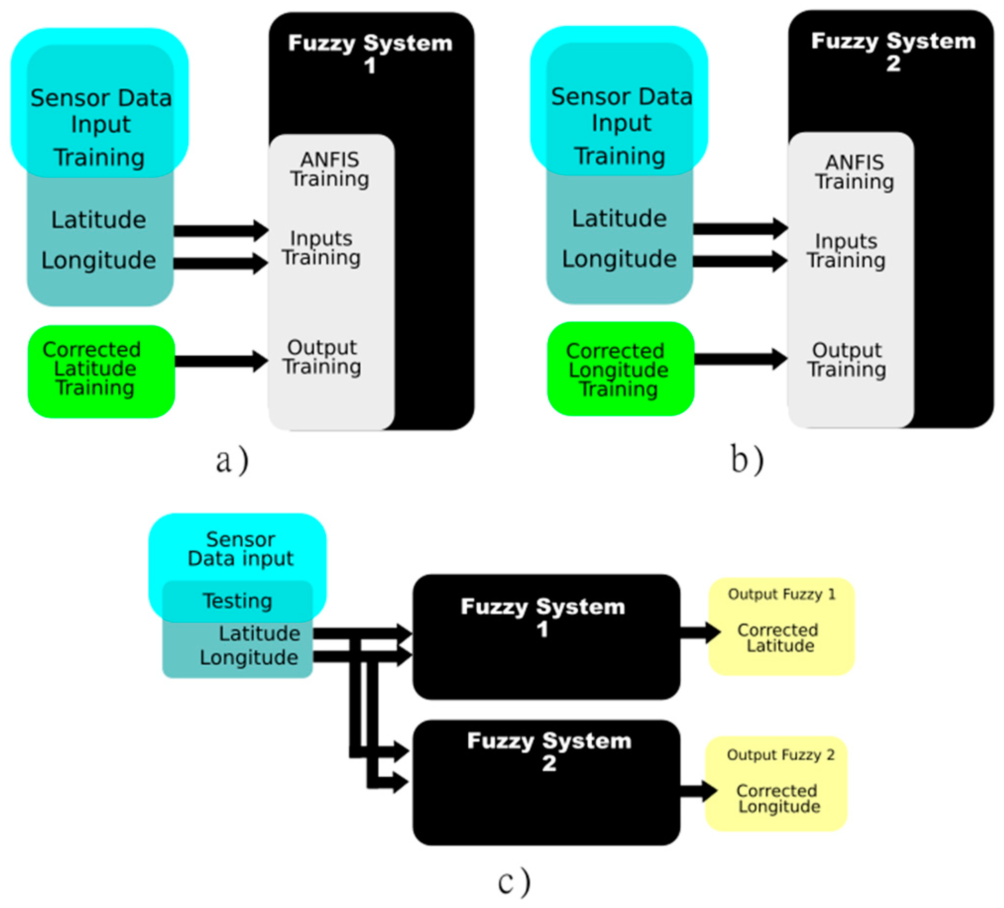
The proposal of the present work consists of implementing a pair of fuzzy systems that have the direct responsibility of correcting the latitude and longitude coordinate coming from the GPS sensor, avoiding complex mathematical operations, and obtaining a complete location system embedded in an electric car. Contrasting with what is found in the state of the art where it is more common to find fuzzy logic as a tool of artificial intelligence complementary to more classical techniques in the subject of location and tracking of land vehicles such as the Kalman filter. For example, in [2], the unscented Kalman filter (UKF) is combined with the unscented H-infinity (UH) filter in order to reduce the accuracy error when tracking the position of a ground vehicle as it travels along a defined route. This system uses fuzzy logic to automatically weight whether the UKF or the UH will act at a given instant along that route, presenting an error reduction of approximately 5.6% in the estimation, with respect to that of the pure UKF, improving the accuracy of the GPS receiver.

In [3], the design of a fuzzy system that adaptively modifies the extended Kalman filter (EKF) noisy covariances by fusing data from GPS, IMU, an odometer (at each wheel) and the mathematical model of the vehicle is shown. In this work, an improvement (on average) in the accuracy of the absolute position of the vehicle of about 49% is shown, making the response of the proposed algorithm superior to that of the original Kalman filter. Similarly, in [4] there is a four-wheeled robot where the EKF is used to fuse data from a GPS, IMU, odometers on the wheels, and additionally a camera on the front of the robot; a fuzzy system is designed to modify the noisy covariances of the EKF. The main objective of this proposal is to strengthen the accuracy in the estimation of the trajectory to be followed by the robot, achieving an average accuracy improvement of 80.6% with respect to the EKF correction. On the other hand, [5] seeks to improve the movement of a two-wheeled robot in environments with many obstacles. This is done by using measurements from a GPS sensor and an adaptive neuro-fuzzy inference system (ANFIS) as control techniques; obtaining a system capable of evading obstacles and estimating the best route for the robot to travel.

In parallel, other artificial intelligence techniques are also currently being applied to improve the response of the Kalman filter. As in [6] where they propose the use of a recurrent neural network (RNN) to adaptively modify the input values of a network real-time kinematic (NRTK) that fuses data from a GPS and an IMU and the kinematic model of the car in real time. This is done in order to improve the tracking of the trajectory of a car with an embedded sensor system, reducing the location accuracy error to 67.71% on average. In [7], the authors use the variation of the Kalman filter, the cubature Kalman filter (CKF), to adaptively modify the noisy covariances creating the strong tracking cubature Kalman filter. The algorithm proposed in this work manages to improve the position estimation of a vehicle with GPS and IMU sensors coupled, obtaining an average error reduction of 56% with respect to the original version of the CFK when traveling along a route. On the other hand, in [8] a classification algorithm is developed that combines a convolutional neural network (CNN) mathematical model of different types of vehicles and data coming from a GPS sensor to analyze the trajectory travelled by the sensor to determine what type of vehicle is making the journey. The authors report a classification accuracy of over 74%.

Again in [9], the authors present a fuzzy logic system capable of determining the position of a moving robot in a shaded indoor environment (such as a tunnel or a covered car park). Using GPS data and analyzing the chromaticity and frequency-component ratio of the LED lights installed in the ceiling and compared to a navigation potential system. The fuzzy system achieves, in the best case, an advantage of up to 89%. Similarly, in [10], a combination of fuzzy logic and optimal control theory is proposed to control the motors of a racing car and achieve its displacement along a specific route without a driver. This is done by taking advantage of the data provided by a GPS sensor, calculating the vehicle’s yaw angle and using the mathematical model of the car. In this work, the authors achieve a 30% improvement in the accuracy of vehicle trajectory tracking. In [11], a GPS sensor is used as a reference and an inertial measurement unit (IMU) delivers data to an inertial navigation system (INS) to reconstruct a trajectory. The INS by itself has a significant error and to reduce it an ANFIS is used which has as inputs the IMU data and the error between the INS and the GPS and as output delivers a corrected estimate of the INS. The authors manage to reduce the INS error by up to 9.83%.

In [12], a GPS receiver delivers data to an extended Kalman filter (EKF) to track the position of a car as it travels along a defined route. The EKF alone is not good at estimating the position of the vehicle when the GPS receives poor signals from the satellites. The authors propose a fuzzy system that adaptively adjusts the internal parameters of the Kalman filter, such as the noisy covariances, to improve its estimates when the GPS has a weak signal. The authors manage to improve vehicle tracking in adverse conditions for the GPS sensor by up to 70%. In [13], by exploiting the fusion of data from an INS and a GNSS sensor attached to a vehicle, the authors present a new fuzzy strong-tracking curbature Kalman filter (FSTCKF) algorithm to improve the CKF response using a fuzzy logic system and reduce the vehicle trajectory estimation error by 72.3%.

On the other hand, in [14], an algorithm is proposed that joins model free adaptive control (MFAC) and particle swarm optimization (PSO) techniques to improve the position tracking of unmanned ground vehicles. For this, they have a GPS, a sensor to measure the angle of rotation of the wheel (which are fused by the mathematical model of the car) and an INS. The authors propose a control algorithm that estimates the heading angle (or direction that the vehicle should have in an instant of time) obtaining a high precision in both the estimation of the angle and the tracking of the vehicle’s path. In contrast, in [15], the authors use ultra-wideband (UWB) technology to improve the localization and tracking accuracy of unmanned ground vehicles (UGV). Three UWB base stations are used as a cluster in a 2D space for localization. Here, by collecting data from multiple tests, they developed an algorithm composed of PSO techniques and genetic algorithms (GA) to implement multiple groups of UWB base stations. The authors report UGV position estimation accuracies between 20 cm and 60 cm. Finally, in [16], they have a GPS sensor and an IMU as input to an extended Kalman filter with an adaptation mechanism to remove noise coming from the IMU and guarantee a better INS response. The authors also develop a deep learning framework with multiple short to long term memory modules (multi-LSTM) to predict the vehicle position increment based on the Gaussian mixture model (GMM) and the Kullback–Leibler (KL) distance. They then combine both algorithms to optimize the estimation of a vehicle’s position achieving an error reduction of up to 93.9%.

In Section 2, the experiments performed are presented; in Section 3, it is shown how the absolute position correction fuzzy system was designed; in Section 4, the design to implement the UKF filter to compare its response with the proposed fuzzy system is exposed; in Section 5, the results are shown with their discussion and finally in Section 6, the conclusions are presented.

2. Materials and Methods

For the experimental development of this work we have a data acquisition system (see Figure 1), which contains the Pmod GPS sensor [17] that receives signals from the GPS satellite system of the United States of America. There is also a Sense HAT [18] nine-axis inertial measurement unit to measure the vehicle’s steering angle for use by the Kalman filter. The data from these sensors is acquired and recorded by a Raspberry Pi 3 using the Python language. The module is coupled to an electric trolley with which several routes were travelled (see Figure 2).

The collected data were processed by the MATLAB tool anfisedit (adaptive neuro-fuzzy inference system) for training and testing the proposed fuzzy algorithms. In the same way, the behavior of the fuzzy systems in the presence of unknown data was evaluated with the help of the evalfis toolbox. The design and implementation process of the proposed fuzzy systems is described below.

2.1. The Data Acquisition System

In Figure 1, we show the modular data acquisition system implemented in this work. The system consists of a GPS Pmod sensor that is used to obtain latitude and longitude coordinates of the current position and a shield Sense HAT for Raspberry to measure the current inclination on the three Pich, Roll, and Yaw axes through its accelerometer. All the register data is stored in CSV format files for post processing on a PC.

To test our system, we traced four routes, which are shown in Figure 2. These routes were traveled four times in order to generate enough data for the training and validation of the fuzzy system.

The red markers in Figure 2 correspond to initial and final points from which the lines that circumscribe the reference are constructed and the blue lines represent the path of the data acquisition module along each route. Parameters such as distance traveled, duration, and velocity are presented in

Table 1. Relevant data of the acquisition stage.

Route	Distance (m)	Time (s)	Velocity (m/s)
(a) 1	282.45736	1020	0.276918
(b) 2	282.9798	840	0.336880
(c) 3	151.8607	480	0.316376
(d) 4	104.3988	420	0.248568

.

From the latitude and longitude data provided by the GPS sensor, we can estimate the distance traveled by means of the Haversines equation [19] as

$$\mathrm{d}=2\cdot r\cdot {\sin }^{-1}\left(M\right)$$

(1)

with r = 6371 km (radius or the earth) and $M=\sqrt{{\sin }^2\left(\frac{{\mathsf{\phi }}_2-{\mathsf{\phi }}_1}{2}\right)+\cos {\mathsf{\phi }}_1\cdot \cos {\mathsf{\phi }}_2\cdot {\sin }^2\left(\frac{{\mathsf{\lambda }}_2-{\mathsf{\lambda }}_1}{2}\right)}$. Here, φ are the latitudes and λ the longitudes obtained from the sensors.

2.2. Approximation Data

On the approximation data, the fuzzy system performs a correction from the GPS data (latitude and longitude). To do this, there is a training stage where, the system indicates the size, proportion, form, or nature of the mentioned correction. In this stage, reference points were established on each route (see red markers on each route of Figure 2) and straight lines were drawn between point and point calculating their equations (see Figure 3).

In Figure 3, a green line represents the reference of each route and the black dashed line represents the data captured by the GPS sensor. Equation (1) is used to calculate the distance between the coordinates given by the GPS sensor and the midpoints of the straight lines that make up the routes (Equations (2) and (3)).

$${\mathsf{\phi }}_{\mathrm{m}}=\frac{{\mathsf{\phi }}_1+{\mathsf{\phi }}_2}{2}$$

(2)

$${\mathsf{\lambda }}_{\mathrm{m}}=\frac{{\mathsf{\lambda }}_1+{\mathsf{\lambda }}_2}{2}$$

(3)

with φ and λ for latitude and longitude respectively.

In Figure 4, it can be observed how the system performs a correction on route 1 from a coordinate point (black point) given by the GPS sensor. The distance of the sensor data to each midpoint of the lines that make up the path of the route is calculated. From the calculated distances (blue lines in Figure 4), we select the smallest one to determine the line of reference to which the sensor data should be corrected or approximated.

Once the minimum distance has been calculated, the data who belongs to the line of reference is evaluated. From this evaluation, the approximation of the GPS sensor data is achieved as it is shown in Figure 5.

The red dots in Figure 5, represent the approximation of the sensor data to the reference and the black dashed line represents the GPS sensor data and the green straight lines represent the reference of each route. Once the corrected coordinate points are obtained, they were stored in matrices for training and validation of the fuzzy systems, which will automatically correct new incoming sensor data. It should be noted that this post-processing stage of the data was done offline using a desktop computer with the characteristics specified Section 2.

This strategy for establishing the fuzzy sets resembles the way a human being would intuitively calculate the distance of his current position with respect to a specific street; the issue of establishing the linguistic variables and their intuitive nature is discussed more extensively in [20,21].

Before using these corrected coordinates (red dots in Figure 5) in the training stage, it is necessary to apply a data cleaning technique such as removing the outliers. The criterion used was the distance between the reference and the corrected latitude and longitude data: when the distance is greater than 3 m then the point is considered an outlier and is removed from the data set to be used for training. It is important to note that the raw data coming directly from the GPS sensor was used in the testing stage.

2.3. Fuzzy System Design

In this work, we use the ANFIS toolbox [22], which allows us to generate a MISO (multiple input, single output) fuzzy inference system based on the Takagi Sugeno method [23]. With this toolbox, the fuzzy system can simultaneously perform a correction from two inputs, latitude and longitude. In this regard, we generated two fuzzy systems one for latitude correction and the other one for longitude correction. Both fuzzy systems receive the same information from the sensor. The data used for training and validation is shown in

Table 2. Datasets for the fuzzy systems.

Route	Training Data	Validation Data	Total
1	751	250	1001
2	645	215	860
3	356	118	474
4	412	102	514

. This is the data collected with the sensor for each route. This is illustrated in Figure 6, where 6a and 6b correspond to the training setup of the two fuzzy systems. Figure 6c represents the system on the testing stage.

From the training we found that the fuzzy systems for latitude and longitude correction were designed with 5 and 3 gaussian membership functions of type two [24], respectively, it is 25 and 9 fuzzy rules for each. For both systems, linear type membership functions were defined at the output. The results of the training stage for both fuzzy systems are shown in

Table 3. ANIFS training output.

Fuzzy System	MF Input Lat	MF Input Lon	MF Output	Fuzzy Rules	RMSE (Train)
Latitude	5 gaussian type 2	5 gaussian type 2	linear	25	$4.29\times {10}^{-7}$
Longitude	3 gaussian type 2	3 gaussian type 2	linear	9	$1.1\times {10}^{-4}$

.

The selection of the membership functions was carried out by means of an optimization process that consisted of varying both, the number of functions for each input and their type (triangular, trapezoidal, Gaussian, and Gaussian type two). From this, we observed the effect at the output for the different configurations and that with the best performance on each fuzzy system is presented in Table 3.

To choose an adequate number on the membership functions that guarantees best compromise between a low error and a minimum number of membership functions, a tuning was performed on each fuzzy system. Multiple tests were launched varying the number of membership functions for each entry in both fuzzy systems, results are presented in Table 3.

After training, MATLAB’s evalfis tool [25] was used to evaluate them with the test data. From the evaluation of both fuzzy systems, two vectors were obtained with the corrected latitude and longitude outputs.

Figure 7 graphically shows the output of each system for the testing data. Figure 7a,b shows the operating range of the fuzzy system correcting latitude and longitude respectively; having as input the GPS sensor data. To compare our results, we implemented the unscented Kalman filter (UKF) and results are presented below.

2.4. Kinematic Model of Car and Tuning of UKF

The UKF takes the data from the inertial measurement unit (IMU) that measures the rotation angle of the front vehicle wheels and the GPS sensor, which estimates the vehicle position located in the center of the axis of the rear wheels as shown in Figure 8.

The land vehicle model is linearized as follows:

$$\dot{\phi }=\phi +s\ast dt\ast \cos \left(\varphi \right)$$

(4)

$$\dot{\lambda }=\lambda +s\ast dt\ast \sin \left(\varphi \right)$$

(5)

$$\dot{\varphi }=\varphi +dt\varphi$$

(6)

$$\dot{s}=s$$

(7)

where $s$ is the vehicle speed (measured by the GPS); $\varphi$ the steering angle; $\phi$ and $\lambda$ correspond to latitude and longitude respectively (also given by the GPS). Analyzing the vehicle model in the state space we have the equation

$$\dot{X}=F\ast X+B\ast u$$

(8)

$$\left[\begin{array}{c}\dot{\phi }\\ \dot{\lambda }\\ \dot{\varnothing }\\ \dot{s}\end{array}\right]=\left[\begin{array}{cccc}1& 0& 0& 0\\ 0& 1& 0& 0\\ 0& 0& 1& 0\\ 0& 0& 0& 0\end{array}\right]\ast \left[\begin{array}{c}\phi \\ \lambda \\ \varnothing \\ s\end{array}\right]+\left[\begin{array}{cc}\sin \left(\varphi \right)dt& 0\\ \cos \left(\varphi \right)dt& 0\\ 0& dt\\ 1& 0\end{array}\right]\ast \left[\begin{array}{c}s\\ \varnothing \end{array}\right]$$

(9)

where $X$ is the vector states used by the UKF and $u$ the vector of inputs from the sensors and those used by the UKF.

Table 4. Tuning of the covariances Q and R of UKF.

#	Q	R
1	$\left(\left[0.1,0.1,\mathrm{rad}\left(350\right),0.1\right]\right)\times {10}^2$	$\left(\left[0.1,-0.1\right]\right)^2$
2	$\left(\left[0.1,0.1,\mathrm{rad}\left(350\right),0.1\right]\right)\times {10}^3$	$\left(\left[0.1,-0.1\right]\right)\times {10}^3$
3	$\left(\left[0.1,0.1,\mathrm{rad}\left(350\right),0.1\right]\right)\times {10}^3$	$\left(\left[0.05,-0.05\right]\right)\times {10}^3$
4	$\left(\left[0.001,0.001,\mathrm{rad}\left(350\right),0.001\right]\right)\times {10}^3$	$\left(\left[0.025,-0.025\right]\right)\times {10}^3$
5	$\left(\left[0.0001,0.0001,\mathrm{rad}\left(350\right),0.0001\right]\right)\times {10}^3$	$\left(\left[0.025,-0.025\right]\right)\times {10}^3$
6	$\left(\left[\mathbf{0.001}, \mathbf{0.001}, rad\left(\mathbf{350}\right), \mathbf{0.001}\right]\right)\times {\mathbf{10}}^{\mathbf{3}}$	$\left(\left[\mathbf{0.025},\mathbf{-}\mathbf{0.025}\right]\right)\times {\mathbf{10}}^{\mathbf{3}}$
7	$\left(\left[0.001,0.001,\mathrm{rad}\left(350\right),0.001\right]\right)\times {10}^3$	$\left(\left[0.025,-0.025\right]\right)\times {10}^3$
8	$\left(\left[0.001,0.001,\mathrm{rad}\left(350\right),0.001\right]\right)\times {10}^4$	$\left(\left[0.025,-0.025\right]\right)\times {10}^4$
9	$\left(\left[0.001,0.001,\mathrm{rad}\left(350\right),0.001\right]\right)\times {10}^5$	$\left(\left[0.025,-0.025\right]\right)\times {10}^5$
10	$\left(\left[0.001,0.001,\mathrm{rad}\left(350\right),0.001\right]\right)\times {10}^6$	$\left(\left[0.025,-0.025\right]\right)\times {10}^6$

shows a synthesis of the optimization process of the UKF to find the values of the noisy covariances that would help to improve the filter response without distorting its output. This process consisted of varying the values of the main diagonals of the Q (process noisy covariance) and R (measurement noisy covariance) matrices of the UKF filter [26] and observing its effect at the filter’s. Here, 10 tests were performed and the one with the best results is shown in row 6 of Table 4.

Equations (10) and (11), show the values of the R and Q covariance matrices for tuning the UKF, highlighting, those that delivered the best correction response of the sensor data.

$$\mathrm{Q}={\left[\begin{array}{cccc}0.001& 0& 0& 0\\ 0& 0.001& 0& 0\\ 0& 0& \mathrm{rad}\left(350\right)& 0\\ 0& 0& 0& 0.001\end{array}\right]}^3$$

(10)

$$\mathrm{R}={\left[\begin{array}{cc}0.025& 0\\ 0& -0.025\end{array}\right]}^3$$

(11)

The final response of the UKF is obtained and shown in Figure 9, where the correction made by the Kalman filter is observed. The difference of this correction with respect to the reference is also observed. For this, the same data of the fuzzy system was used (Table 2).

Figure 9 shows the reference in green, the dashed black line represents the GPS sensor data and the purple line corresponds to the data correction produced by the Kalman filter.

Additionally, the UKF has a scaling parameter kappa (κ) whose value is 3-L (where L is the length of the variable to be analyzed, i.e., 2); Beta (β) that incorporates a priori knowledge of the variable to analyze, in this case it is assumed that the variables have a gaussian distribution being then, β = 2. Finally, alpha (α) is a parameter that indicates the propagation through the mean of the variable to be analyzed and it varies between 1 and $1\times {10}^{-4}$, in our case we set this value to 0.01. The selection of these parameters is based on the recommendations made in [27] and a tuning process to find the most optimal value. The following section shows, graphically and numerically, the results obtained in both the fuzzy system and those of the UKF, also a comparison of the two systems is presented.

3. Results

3.1. Analysis of Results with Our Own Dataset

To facilitate the description of results, we abbreviate fuzzy position correction as FPC. The comparison between the UKF response (purple) and our method (blue) is graphically depicted for each route in Figure 10. In such figure both results are also contrasted with the reference (green). These results are further quantified numerically by means of the RMSE and presented in

Table 5. RMSE results of the UKF and fuzzy system (FPC).

Route	UKF: RMSE (m)	Fuzzy (FPC): RMSE (m)
1	$1.989\times {10}^{-4}$	$1.490\times {10}^{-4}$
2	$7.539\times {10}^{-4}$	$2.289\times {10}^{-4}$
3	$4.865\times {10}^{-4}$	$2.926\times {10}^{-4}$
4	$2.698\times {10}^{-4}$	$2.510\times {10}^{-4}$

. From the RMSE results observed in Table 5, it is evident that the proposed fuzzy system improves the absolute vehicle location accuracy by 26% for route 1, 69.2% for route 2, 40% for route 3, and 7% for route 4, compared to the UKF response.

Figure 11 shows the error (in meters) between the UKF output and the reference (purple), as well as the output of the fuzzy systems and the reference (blue graph). This graph shows that, for some sections of each trajectory, the error of the fuzzy systems is smaller than that observed in the UKF, in others the opposite is true or they are similar. This shows that the designed fuzzy systems have a consistent response and offer a competitive alternative to the UKF.

It is important to mention that even if the response is similar in most of the cases, the UKF performs a fusion of data from four inputs (angle of rotation of the front wheels, vehicle speed, latitude, and longitude) to be able to deliver an estimate of the position of the vehicle; while the FPC only needs two inputs, those of the GPS (latitude, longitude), to deliver a better estimate.

Also, the UKF filter needs parameters tuning to obtain the optimal R and Q covariance values for a more accurate estimate, in addition to the behavior of the random variables processed by this algorithm setting the values of κ, β, and α. In contrast, the proposed FPC system is not dependent on any parameters since it only needs the latitude and longitude data given by the GPS to operate.

Table 6. Statistical performance tests (mean and variance).

UKF
Route	Mean (m)	$\mathrm{Variance}(m^2$)
1	$1.366\times {10}^{-2}$	$4.764\times {10}^{-5}$
2	$5.744\times {10}^{-2}$	$1.297\times {10}^{-3}$
3	$3.755\times {10}^{-2}$	$1.039\times {10}^{-4}$
4	$1.736\times {10}^{-2}$	$1.233\times {10}^{-4}$
FPC (Fuzzy system)
Route	Mean (m)	$\mathrm{Variance}(m^2$)
1	$1.300\times {10}^{-2}$	$4.983\times {10}^{-5}$
2	$5.829\times {10}^{-2}$	$1.315\times {10}^{-3}$
3	$3.766\times {10}^{-2}$	$9.634\times {10}^{-5}$
4	$1.852\times {10}^{-2}$	$1.114\times {10}^{-4}$

reports the statistical tests of media and variance that serve as a comparison of the performance of the UKF and the proposed fuzzy FPC system. For this calculation, the equation 1 of the haversines is used to find the distance of each point of the output of the fuzzy system FPC and the UKF respect to the reference in each route.

The variance represents the degree of dispersion of the data of a variable with respect to its mean (in the case of a Gaussian distribution). From Table 6, it is observed that in the variance calculation test the error variable of the FPC fuzzy system is slightly greater for the first two routes respect to the variance of the UKF. From this result, it can be inferred that—as expected—the UKF has more advantage to correct certain data than the fuzzy system and vice versa.

3.2. Analysis of Results with Public Dataset

In order to validate the robustness of our method, the public GPS trajectories data set [28,29] containing about 163 routes or trajectories travelled by car on the streets of Brazil and recorded with the Android application “Go! Track” was used. This database is perfectly adapted to the design needs of the proposed fuzzy systems and gives the possibility to test its performance with data that were not taken by the acquisition system shown in Section 2.1 and under poorly controlled conditions.

For the test, two random paths were chosen from the dataset and one of them was used to retrain the designed fuzzy systems (see Figure 12). This retraining is necessary due to the fact that the coefficients of the Gaussian functions must fit the new data and the fuzzy systems can perform their task.

Subsequently, the second route (see Figure 13) was used to validate the performance of the fuzzy systems under these new conditions. This data was not used in the training.

Finally, in Figure 14 the response of the proposed fuzzy systems to the new data can be seen. The green graph represents the reference of the route, the black dashed line contains the input data coming from the sensor (in this case, the data collected by the Go!Track app), the red dots are the data calculated with the strategy seen in Section 2.2 and finally the blue dots contain the output of the fuzzy systems.

The purpose of the fuzzy systems is to get the data represented by the dashed black line as close as possible to the reference (green plot), in other words, the closer the blue are to the red dots, the better their performance will be. The red boxes in Figure 14 highlight two segments of the route where the correction made by the fuzzy systems is most noticeable.

Figure 15 shows the error (in meters), between the sensor measurements and the reference (green graph); as well as the error between the output of the fuzzy systems and the reference (in red). From this image, it can be seen that—for most of the data—there is a reduction of the error when the proposed fuzzy systems are in action.

Table 7. RMSE reference vs. sensor and fuzzy system (FPC).

RMSE Sensor vs. Ref (m)	RMSE: Fuzzy (FPC) vs. Ref (m)
$5.51\times {10}^{-4}$	$5.250\times {10}^{-4}$

shows how the RMSE of the fuzzy system outputs is lower than the error of the sensors compared to the reference.

4. Discussion

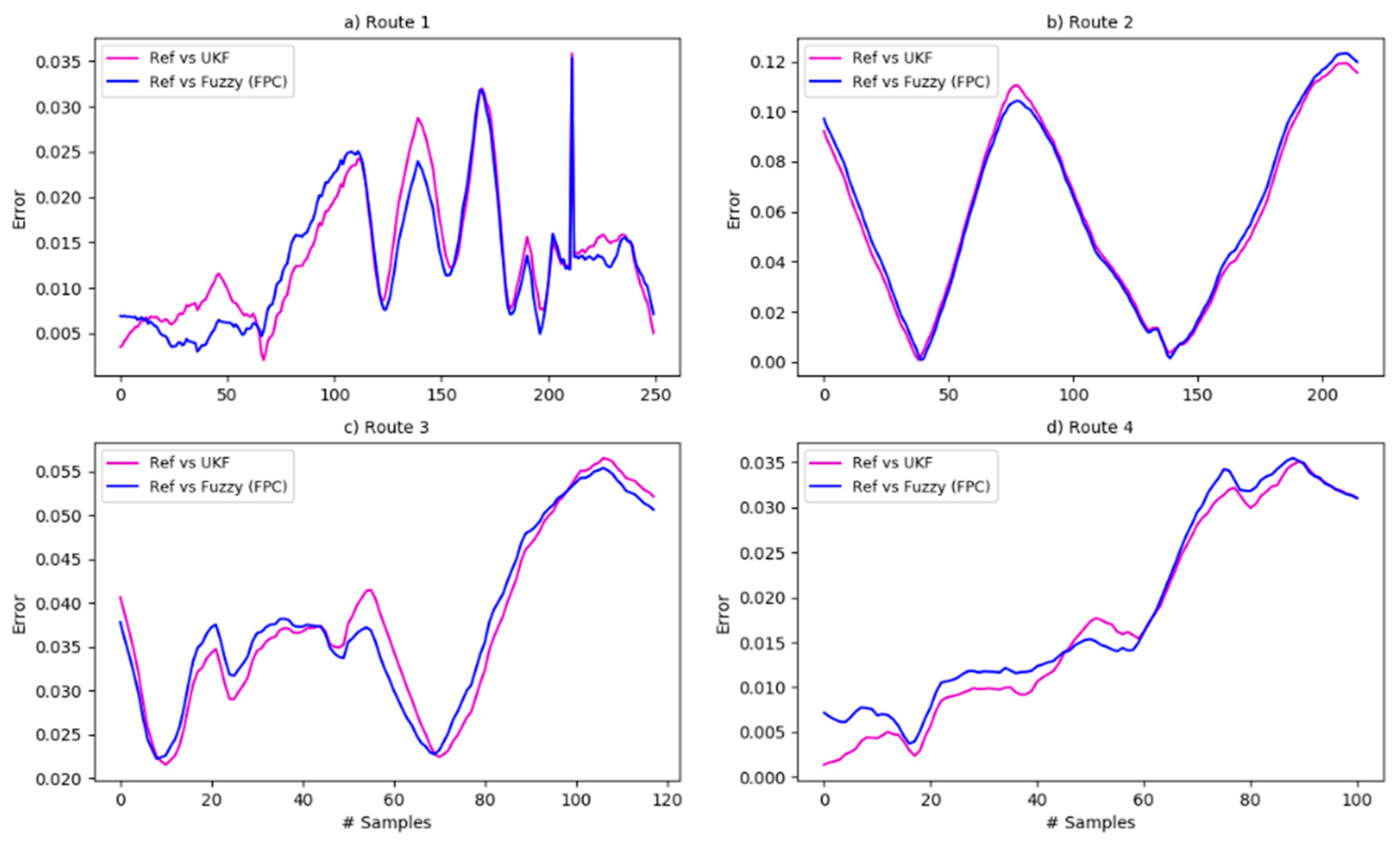
According to the results, the Kalman filter manages to reduce errors with decent performance but needs—as input—data to the covariance matrix that implicitly contains information on noise parameters. On the other hand, the fuzzy system managed to reduce the error in a better way without knowing the type of noise of the system because it was trained in the data region, making it easier and cheaper to implement with respect to works found in the state of the art. The main disadvantage is that, in order to better exploit the performance of the systems, retraining needs to be deployed in order to adjust the parameters of the membership functions when they are tested in geographical areas that are far away from the original data. The main limitation of the proposed fuzzy systems is that: if the error in the GPS measurements is too large, the correction of the GPS measurements will no longer be as effective.

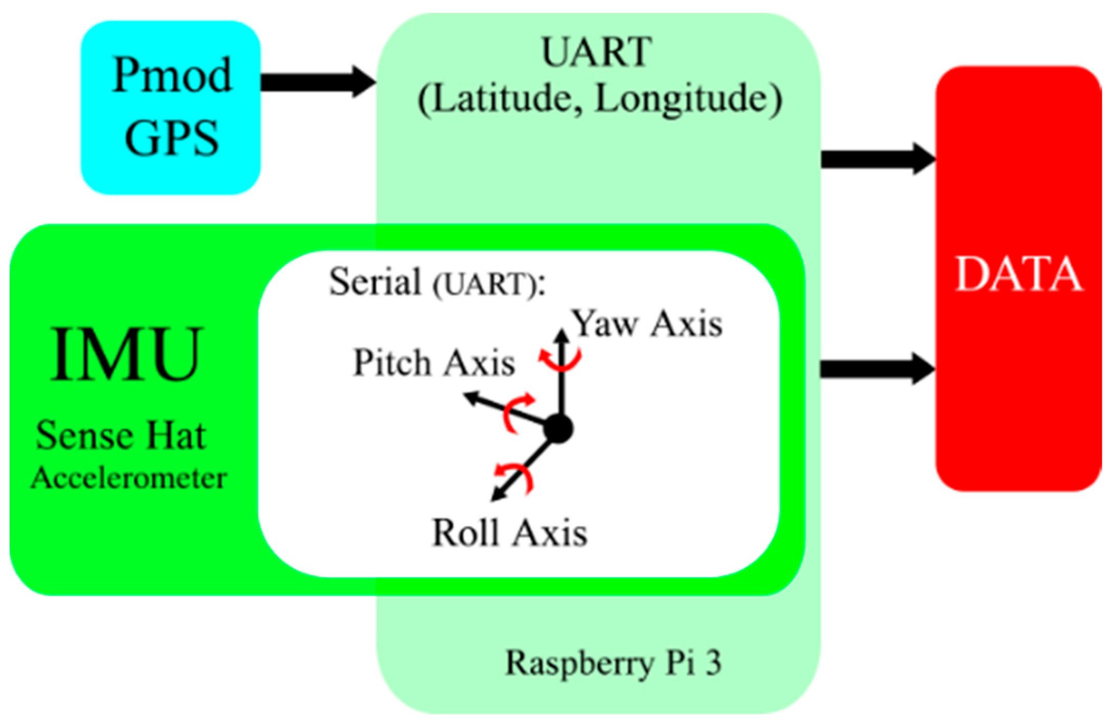
An own data set was collected to take advantage of the data acquisition system (implemented and described in Section 2.1) since the characteristics of the sensors are known, such as the sampling period and the precision of each one, facilitating the post-processing calculations and the use of the information in different applications. Similarly, as the central limit theorem states, the more data that can be collected on a phenomenon, the more the distribution function that describes it will approximate the normal function and most of the data will be clustered around the mean. As shown in

Table 8. RMSE: reference vs. output fuzzy system (FPC).

Dataset	RMSE: Fuzzy (FPC) vs. Ref (m)
Own	$2.510\times {10}^{-4}$
Brazil [28,29]	$5.250\times {10}^{-4}$

, the RMSE of both data sets is similar, being lower for the eigendata. Comparing these values with the information in Table 6, it can be said that they are around the mean of the latitude and longitude variables.

In

Table 9. Maximum accuracy comparison over Kalman filter.

Algorithm	Maximum Accuracy over Kalman Filter (%)
FPC	69.2
AFUKHF [2]	56.14
FI-AKF [3]	58.48
Cons.T2FKF [26]	67.53

, a numerical comparison between the accuracy (concerning the Kalman filter response) of the developed algorithm (FPC) and the reported in references [2,3,26] is presented.

As shown in Table 9, the proposed algorithm has a maximum accuracy, concerning the Kalman Filter, higher than that reported in the papers compared. Although, this accuracy is reduced depending on the route being evaluated (as mentioned above).

5. Conclusions

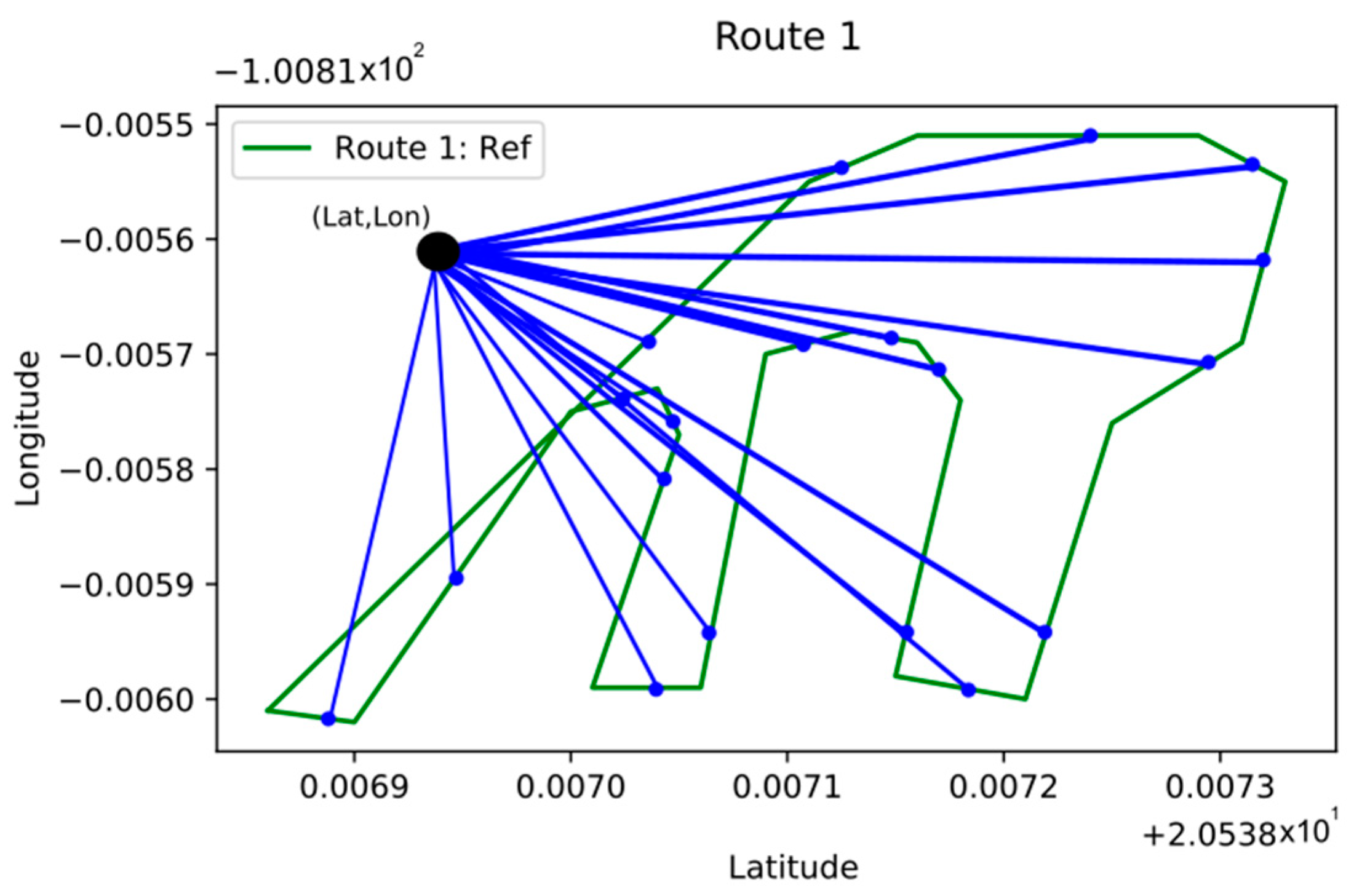
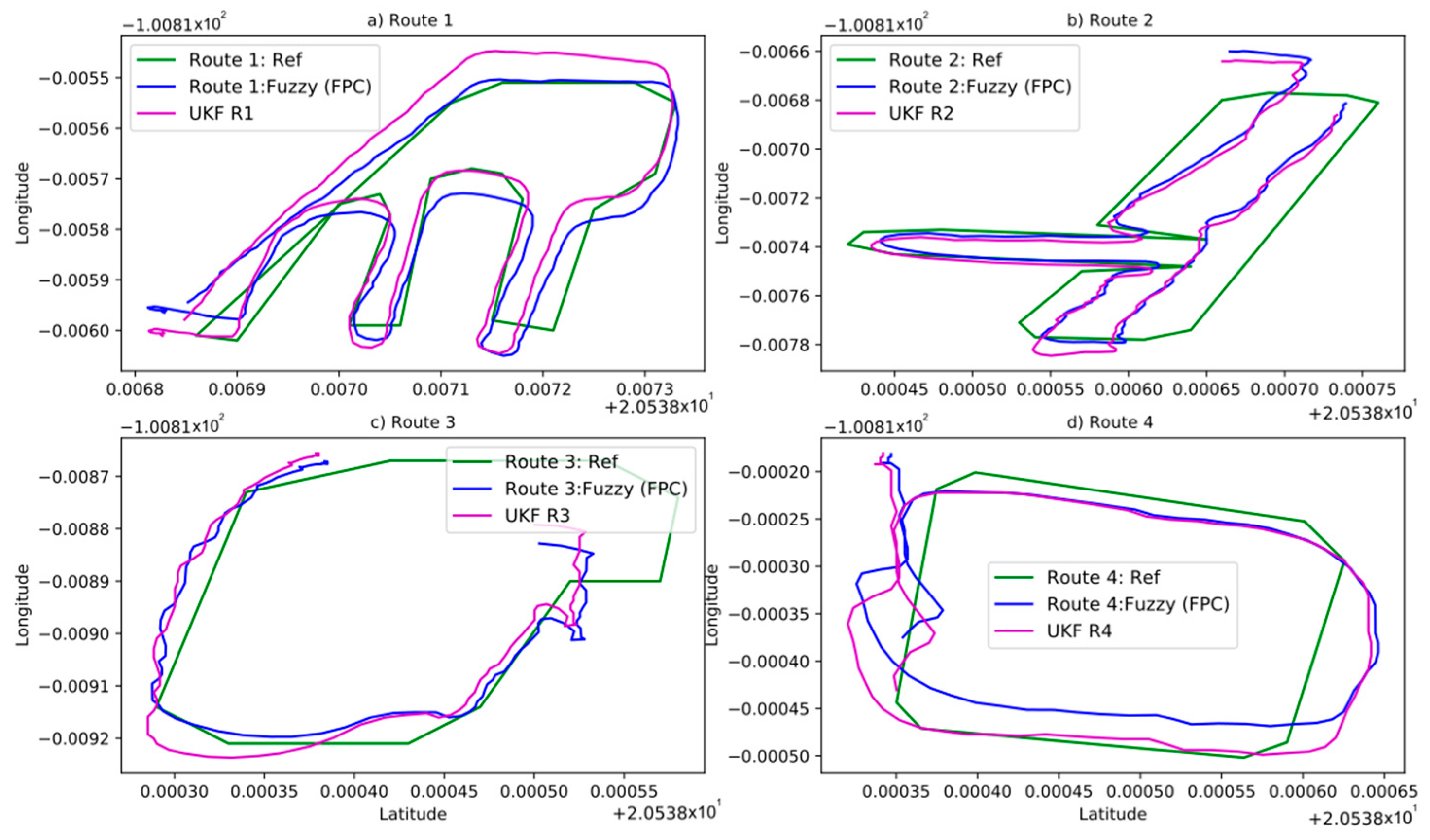
The proposed FPC fuzzy system delivers competitive GPS data correction with the UKF response which is less dependent on tuning parameters, making it as easy (in terms of processing cost) to use and implement on mobile platforms. The proposed fuzzy system (FPC) emulates the way in which a human being describes the shape of a route through lines, so the calculation of these lines is used to approximate the sensor data to the reference.

The response of the fuzzy systems developed in this article improves the accuracy by up to 69.2% to determine the absolute position of a ground vehicle with respect to the classical techniques in this subject such as the UKF. Being highly competitive with techniques developed in the works presented in [2,3,26] (see Table 9). In addition, our method is less dependent on parameters and sensors, since it only uses GPS data and the reference for design.

Despite improving the response of the UKF, the proposed fuzzy system is limited to the region of the GPS map for which it was trained; that is, if the inputs are extremely different from the data the system was trained in, the FPC prediction will have a large errors. To solve this, it is necessary to collect a greater amount of data covering a wider region of the map to retrain the FPC system and expand its scope. Despite this, something similar happens with the UKF because the covariances R and Q must be re-tuned when the data changes dramatically.

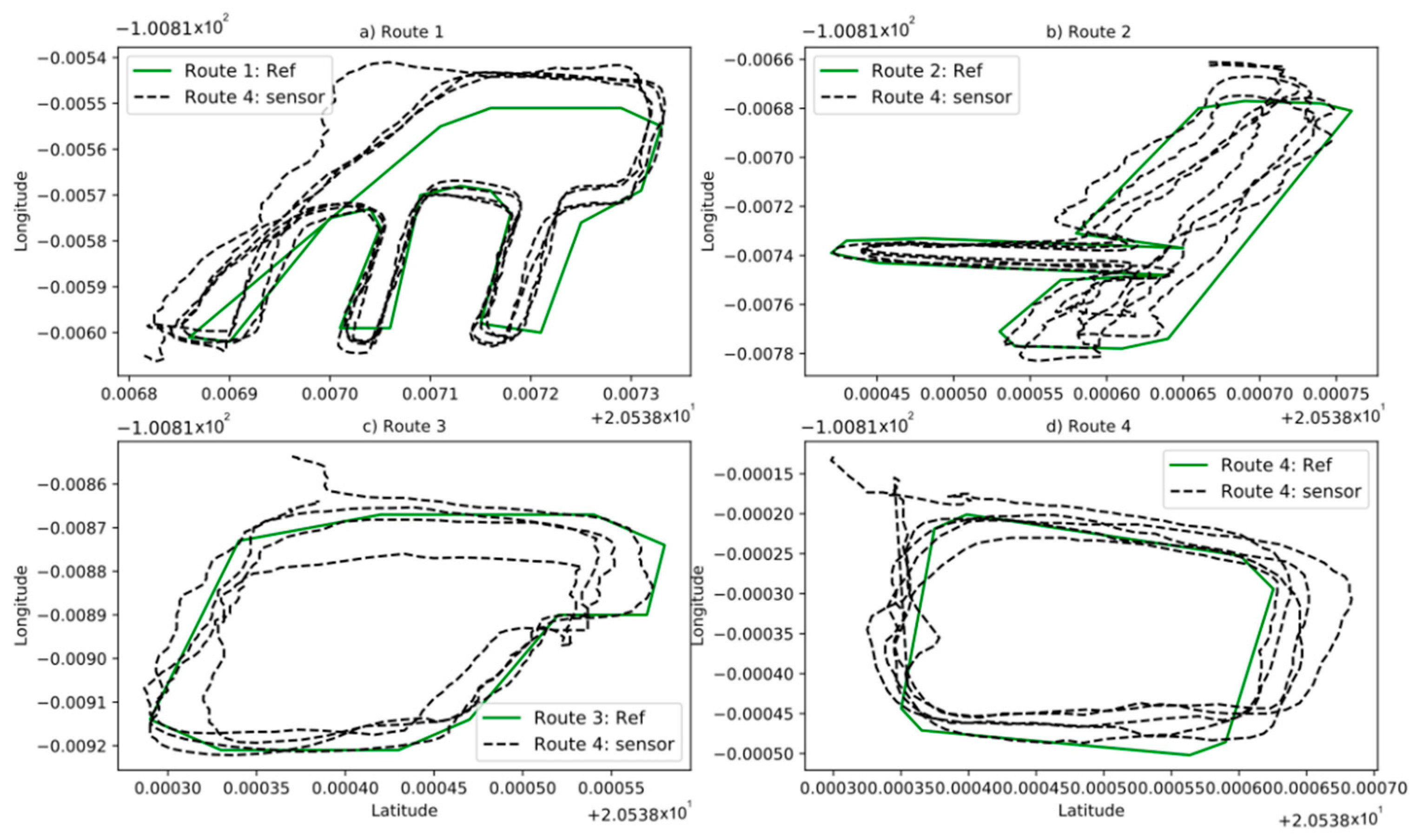
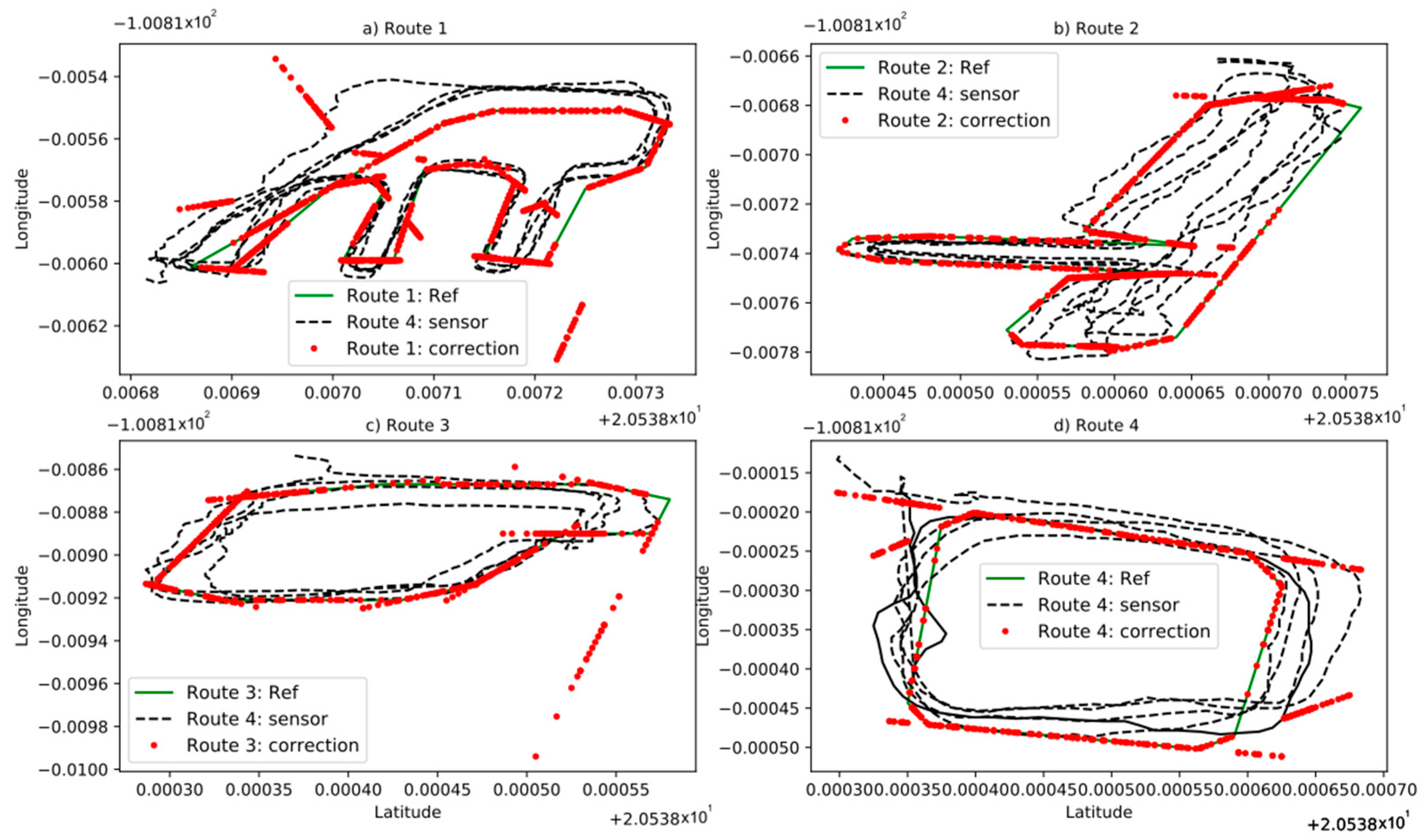
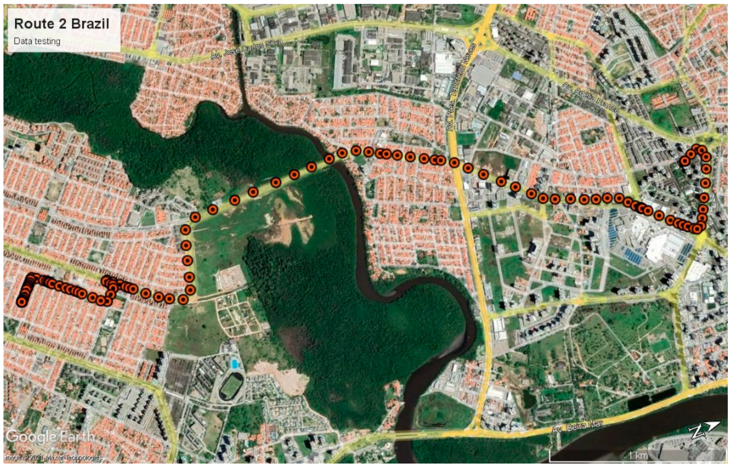
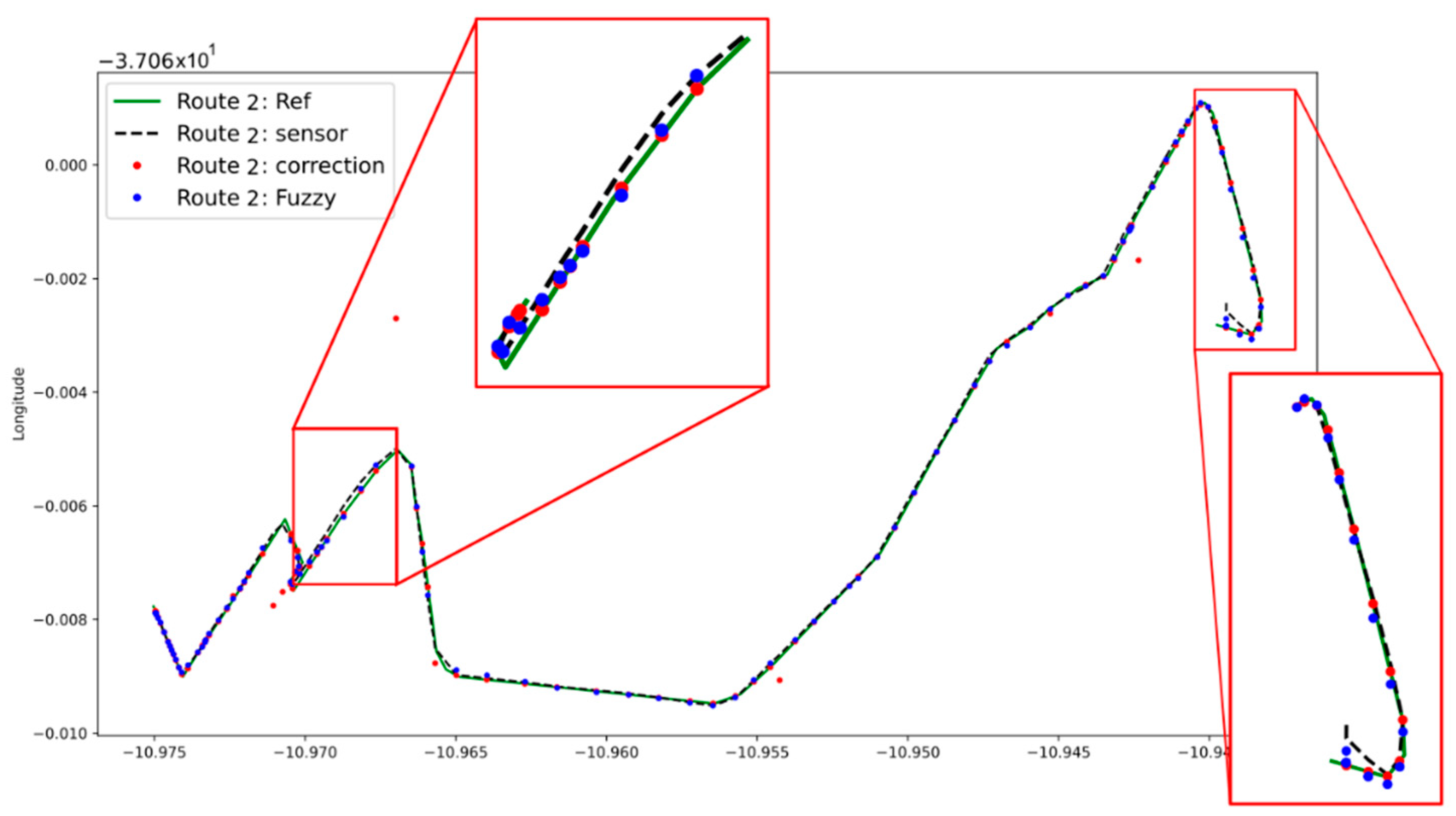
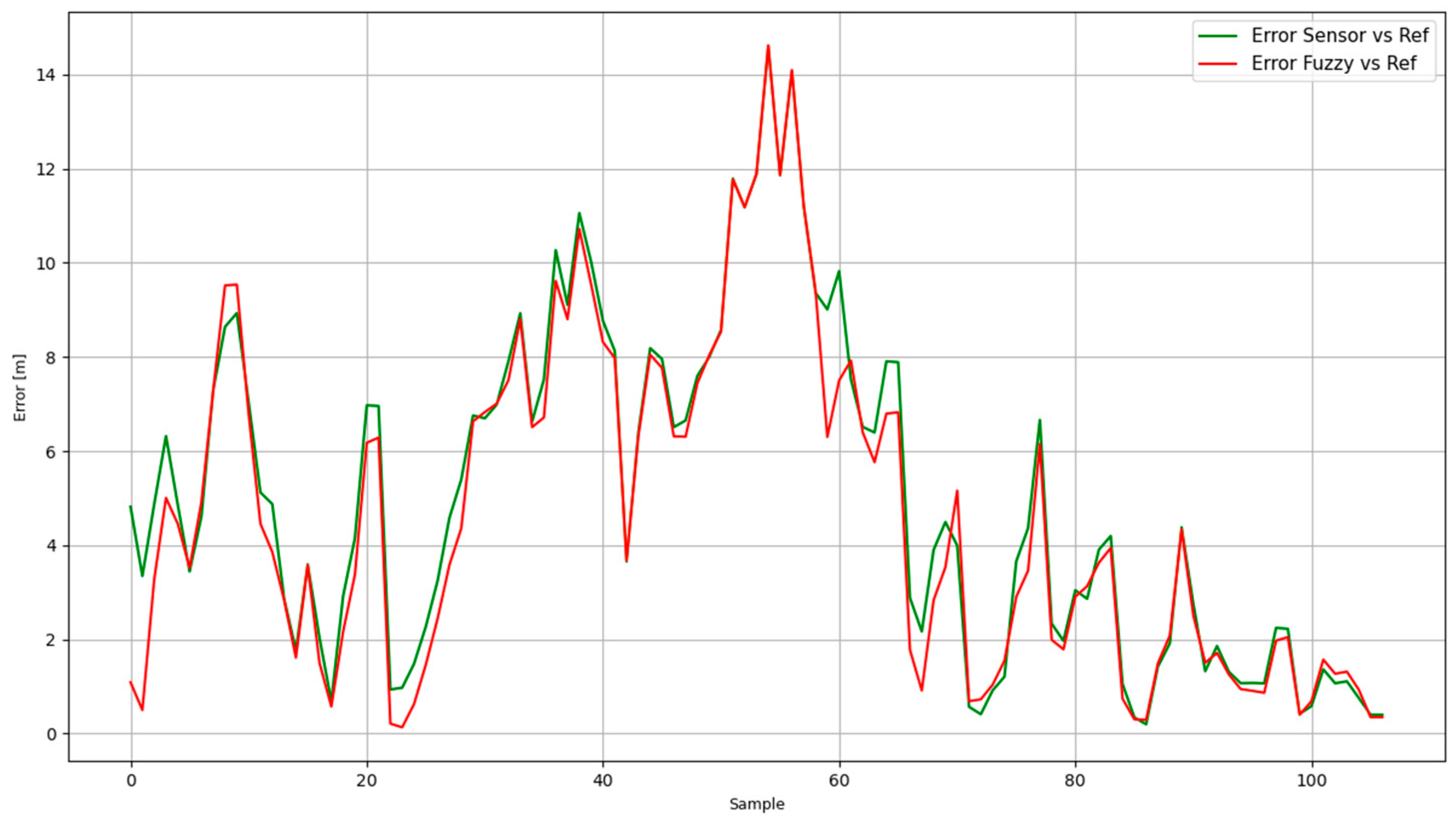
The proposed fuzzy systems were tested on a public dataset [28,29], having a favorable performance under poorly controlled conditions both in the way of acquiring the data and in the geographical area where they were collected. As shown in Figure 14, Figure 15, and Table 7.

One of the points of improvement (in future work) for the proposed fuzzy systems is to achieve generalization of their response. This issue can be approached from two different points of view. The first one can be the collection and processing of the largest number of routes travelled with the GPS sensor to make a more complete training of the systems; the second one is to implement fuzzy systems whose training is online, that is, that the fuzzy systems are trained as the data from the GPS sensor arrives when a route is travelled.

6. Recommendations

In order to successfully reproduce this work, the data must be compiled in a CSV file whose first and second column must be the latitude and longitude data respectively coming from the GPS sensor. In a third and fourth column should be the latitude and longitude data corrected using the technique explained in Section 2.2. To achieve the data correction seen in Section 2.2, it is necessary to plot each new route in Google maps to extract the latitude and longitude points of each corner of the routes and obtain the line equations between each pair of corners.

One of the limitations of the proposed systems is generalization, as re-training is necessary when testing in geographical areas far away from the original data. This is necessary to readjust the parameters of the membership functions to the new data. The combination of MATLAB’s ANFIS and GENFIS tools facilitates the task of deploying multiple training of fuzzy systems and accelerates the design process.

References

1. Fatima, B.; Amine, C.M.; Bekr, A. A Neuro-Fuzzy Inference Model for Breast Cancer Recognition. Int. J. Comput. Sci. Inf. Technol. 2012, 4, 163–173. [Google Scholar] [CrossRef]
2. Tehrani, M.; Nariman-Zadeh, N.; Masoumnezhad, M. Adaptive Fuzzy Hybrid Unscented/H-Infinity Filter for State Estimation of Nonlinear Dynamics Problems. Trans. Inst. Meas. Control 2019, 41, 1676–1685. [Google Scholar] [CrossRef]
3. Woo, R.; Yang, E.-J.; Seo, D.-W. A Fuzzy-Innovation-Based Adaptive Kalman Filter for Enhanced Vehicle Positioning in Dense Urban Environments. Sensors 2019, 19, 1142. [Google Scholar] [CrossRef] [Green Version]
4. Zhu, J.; Tang, Y.; Shao, X.; Xie, Y. Multisensor Fusion Using Fuzzy Inference System for a Visual-IMU-Wheel Odometry. IEEE Trans. Instrum. Meas. 2021, 70, 2505216. [Google Scholar] [CrossRef]
5. Gharajeh, M.S.; Jond, H.B. Hybrid Global Positioning System-Adaptive Neuro-Fuzzy Inference System based autonomous mobile robot navigation. Robot. Auton. Syst. 2020, 134, 103669. [Google Scholar] [CrossRef]
6. Kim, H.-U.; Bae, T.-S. Deep Learning-Based GNSS Network-Based Real-Time Kinematic Improvement for Autonomous Ground Vehicle Navigation. J. Sens. 2019, 2019, 3737265. [Google Scholar] [CrossRef]
7. Shen, C.; Zhang, Y.; Guo, X.; Chen, X.; Cao, H.; Tang, J.; Li, J.; Liu, J. Seamless GPS/Inertial Navigation System Based on Self-Learning Square-Root Cubature Kalman Filter. IEEE Trans. Ind. Electron. 2021, 68, 499–508. [Google Scholar] [CrossRef]
8. Dabiri, S.; Marković, N.; Heaslip, K.; Reddy, C.K. A deep convolutional neural network based approach for vehicle classification using large-scale GPS trajectory data. Transp. Res. Part C Emerg. Technol. 2020, 116, 102644. [Google Scholar] [CrossRef]
9. Jeong, J.-H.; Park, K. Numerical Analysis of 2-D Positioned, Indoor, Fuzzy-Logic, Autonomous Navigation System Based on Chromaticity and Frequency-Component Analysis of LED Light. Sensors 2021, 21, 4345. [Google Scholar] [CrossRef] [PubMed]
10. Li, G.; Zhang, S.; Liu, L.; Zhang, X.; Yin, Y. Trajectory Tracking Control in Real-Time of Dual-Motor-Driven Driverless Racing Car Based on Optimal Control Theory and Fuzzy Logic Method. Complexity 2021, 2021, 5549776. [Google Scholar] [CrossRef]
11. Duan, Y.; Li, H.; Wu, S.; Zhang, K. INS Error Estimation Based on an ANFIS and Its Application in Complex and Covert Surroundings. ISPRS Int. J. Geo-Inf. 2021, 10, 388. [Google Scholar] [CrossRef]
12. Farhad, M.A.; Mosavi, M.R.; Abedi, A.A. Fully Adaptive Smart Vector tracking of Weak GPS Signals. Arab. J. Sci. Eng. 2021, 46, 1383–1393. [Google Scholar] [CrossRef]
13. Chang, Y.; Wang, Y.; Shen, Y.; Ji, C. A new fuzzy strong tracking cubature Kalman filter for INS/GNSS. GPS Solut. 2021, 25, 120. [Google Scholar] [CrossRef]
14. Jiang, Y.; Xu, X.; Zhang, L. Heading tracking of 6WID/4WIS unmanned ground vehicles with variable wheelbase based on model free adaptive control. Mech. Syst. Signal Process. 2021, 159, 107715. [Google Scholar] [CrossRef]
15. Wu, Y.; Ding, S.; Ding, Y.; Li, M. UWB Base Station Cluster Localization for Unmanned Ground Vehicle Guidance. Math. Probl. Eng. 2021, 2021, 6639574. [Google Scholar] [CrossRef]
16. Liu, J.; Guo, G. Vehicle Localization During GPS Outages with Extended Kalman Filter and Deep Learning. IEEE Trans. Instrum. Meas. 2021, 70, 7503410. [Google Scholar] [CrossRef]
17. Pmod GPS Reference Manual; Digilent Inc.: Pullman, WA, USA. Available online: https://reference.digilentinc.com/reference/pmod/pmodgps/reference-manual (accessed on 23 September 2021).
18. Raspberry, Documentation, Hardware, Sense Hat. “Shaun the Sheep” and “Farmageddon” Elements Are © 2019 Aardman and Studiocanal SAS. Available online: https://www.raspberrypi.org/documentation/hardware/sense-hat/ (accessed on 23 September 2021).
19. Sofwan, A.; Soetrisno, Y.A.A.; Ramadhani, N.P.; Rahmayani, A.; Handoyo, E.; Arfan, M. Vehicle Distance Measurement Tuning using Haversine and Micro-Segmentation. In Proceedings of the 2019 International Seminar on Intelligent Technology and Its Applications (ISITIA), Surabaya, Indonesia, 28–29 August 2019; pp. 239–243. [Google Scholar] [CrossRef]
20. Bakbak, D.; Uluça, V. Multicriteria decision-making method using the cosine vector similarity measure under intuitionistic trapezoidal fuzzy multi-numbers in architecture. In Proceedings of the 6th International Multidisciplinary Studies Congress (Multicongress’ 19), Gaziantep, Turkey, 1 August 2019. [Google Scholar]
21. Uluçay, V.; Deli, I.; Şahin, M. Trapezoidal fuzzy multi-number and its application to multi-criteria decision-making problems. Neural Comput. Appl. 2018, 30, 1469–1478. [Google Scholar] [CrossRef]
22. ANFIS: Adaptive Neuro Fuzzy Inference System. The Math-Works, Inc.: USA 1994–2018. Available online: https://www.mathworks.com/help/fuzzy/anfis.html (accessed on 23 September 2021).
23. Kukolj, D. Design of adaptive Takagi–Sugeno–Kang fuzzy models. Appl. Soft Comput. 2002, 2, 89–103. [Google Scholar] [CrossRef]
24. Bergsten, P.; Palm, R.; Driankov, D. Observers for Takagi-Sugeno fuzzy systems. IEEE Trans. Syst. Man Cybern. Part B (Cybern.) 2002, 32, 114–121. [Google Scholar] [CrossRef]
25. evalfis: Evaluate Fuzzy Inference System. The Math-Works, Inc.: USA 1994–2018. Available online: https://www.mathworks.com/help/fuzzy/evalfis.html (accessed on 23 September 2021).
26. Rafatnia, S.; Nourmohammadi, H.; Keighobadi, J. Fuzzy-adaptive constrained data fusion algorithm for indirect centralized integrated SINS/GNSS navigation system. GPS Solut. 2019, 23, 62. [Google Scholar] [CrossRef]
27. Jeffrey, S.J.; Uhlmann, K. New extension of the Kalman filter to nonlinear systems. In Proceedings of the Signal Processing, Sensor Fusion, and Target Recognition, Orlando, FL, USA, 21–25 April 1997; Volume 3068, pp. 182–193. [Google Scholar]
28. Cruz, M.O.; Macedo, H.; Guimaraes, A. Grouping Similar Trajectories for Carpooling Purposes. In Proceedings of the 2015 Brazilian Conference on Intelligent Systems (BRACIS), Natal, Brazil, 4–7 November 2015; pp. 234–239. [Google Scholar]
29. Dua, D.; Graff, C. UCI Machine Learning Repository. University of California, School of Information and Computer Science: Irvine, CA, USA; Available online: http://archive.ics.uci.edu/ml (accessed on 3 November 2021).
Figure 1. Acquisition data system.
Mathematics 09 02818 g001
Figure 2. Test routes: (a) route 1, (b) route 2, (c) route 3, (d) route 4.
Mathematics 09 02818 g002
Figure 3. Sensor data and reference, (a) route 1, (b) route 2, (c) route 3, (d) route 4.
Mathematics 09 02818 g003
Figure 4. Distance’s estimation from a point to the line.
Mathematics 09 02818 g004
Figure 5. Data correction, (a) route 1, (b) route 2, (c) route 3, (d) route 4.
Mathematics 09 02818 g005
Figure 6. Fuzzy system design, (a) Fuzzy system 1 (training): Latitude; (b) Fuzzy system 2 (training): Longitude; (c) Testing both fuzzy systems.
Mathematics 09 02818 g006
Figure 7. Fuzzy systems testing, (a) Fuzzy system 1 (testing): Latitude; (b) Fuzzy system 2 (testing): Longitude.
Mathematics 09 02818 g007
Figure 8. Vector diagram of the car model.
Mathematics 09 02818 g008
Figure 9. Sensor data vs. UKF response. (a) route 1, (b) route 2, (c) route 3, (d) route 4.
Mathematics 09 02818 g009
Figure 10. Reference (green) vs. FPC response (blue) vs. UKF (magenta). (a) route 1, (b) route 2, (c) route 3, (d) route 4.
Mathematics 09 02818 g010
Figure 11. Error: reference vs. fuzzy systems response vs. UKF. (a) route 1, (b) route 2, (c) route 3, (d) route 4.
Mathematics 09 02818 g011
Figure 12. Route 1: data training, Brazil dataset.
Mathematics 09 02818 g012
Figure 13. Route 2: data testing, Brazil dataset.
Mathematics 09 02818 g013
Figure 14. Route 2: Fuzzy systems output.
Mathematics 09 02818 g014
Figure 15. Error: reference vs. sensor (green) and reference vs. fuzzy systems response (red).
Mathematics 09 02818 g015