Mathematics Model for 6-DOF Joints Manipulation Robots

Abstract

A universal solution to an applied problem related to the study of deviations occurring in the joints of manipulation robots, for example, due to elastic deformations or gaps in them, is proposed. A mathematical (dynamic) model obtained by the Lagrange–Euler method is presented, making it possible to investigate such deviations. Six generalized coordinates, three linear and three angulars, were used to describe the variations of each joint in the dynamic model. This made it possible to introduce into consideration joints with six degrees of freedom (6-DOF joints). In addition, mathematical models for external forces acting on the links of manipulation robots are presented. When composing matrices of coefficients of equations of motion, elements identically equal to zero were excluded, which significantly increased the computational efficiency of these equations. The dynamic model based on the obtained equations can be used in the computer simulation of manipulation robots.

1. Introduction

The mechanisms of manipulation robots are multi-link spatial kinematic structures. Such kinematic systems contain links that are sequentially connected by joints with one degree of freedom, forming open kinematic chains. As a rule, the rigid body model is used for the links [1].

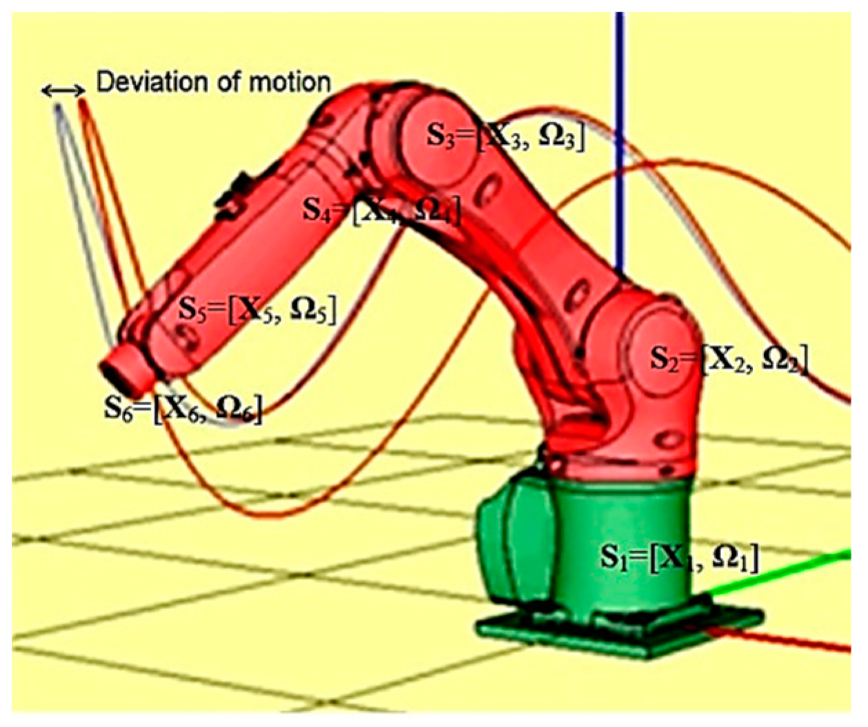
Many works have been devoted to the equations of motion for manipulation robots, modeled by both rigid and elastic links [1,2,3,4,5,6,7,8,9,10,11,12,13,14,15,16,17,18,19,20,21,22,23,24,25]. However, the use of these equations to substantiate the action of real manipulation robots, as a rule, is complicated because of the arising deviations from the given programmed action (Figure 1). Describing such variations is complicated due to the total influence of deviations in each joint. Sometimes, the mobility of the joints is increased artificially by introducing fictitious links with zero mass. That can allow taking such variations into account.

There could be various reasons for the deviations in joints’ design. For example, deviations arising from inaccuracies in the parts’ manufacturing and their subsequent fitting are the primary geometric deviations. Primary geometric deviations increase due to wear and damage to parts of mechanisms during their operation. The ambient temperature can also have an impact. Such deviations do not change as the robots move. There are unique methods for their correction [18,19].

Changing geometric deviations in the joints of manipulation robots are, as a rule, small elastic deformations, leading to a displacement of the joints relative to their undeformed positions. The presence of gaps in the hinges also leads to the appearance of varying geometric deviations. Such deviations can be both angular and linear.

Positioning deviations are considered separately. These deviations reflect the variations of the principal coordinates that provide the functionality of the joints. Positioning deviations occur due to small elastic deformations in the transmission mechanisms and the drive. Determination of such variations was considered in [4,5,6,7], where different methods allowed distinguishing slowly varying (quasi-static) elastic deviations and rapidly changing deviations associated with emerging elastic vibrations.

Modern simulations are a powerful tool in various scientific fields, including robotics, agriculture, education (EdTech), FinTech, and material science [26,27,28,29,30,31,32,33,34,35,36,37,38]. To develop computer simulation approaches, the theoretical basics for them need to be developed and improved. The purpose of the research reflected in this article is to create a comprehensive approach to account for the influence of geometric deviations in robotics and develop a mathematical apparatus for composing equations of motion of manipulation robots reflecting such variations.

In this paper, an attempt is made to create a universal dynamic model that allows taking into account all possible geometric deviations in the joints of manipulation robots that occur during their movement. Furthermore, based on the experimentally obtained data on the nature of variations in the robot’s joints, it allows determining the forces and moments corresponding to these deviations. Such a dynamic model will differ from the previously proposed mathematical models by a greater breadth of coverage of various variations and can be used in computer simulation systems of manipulation robots.

2. Problem Statement

In this paper, we have proposed using joints with six degrees of freedom (6-DOF) [25] to determine the changing geometric deviations that arise when manipulating the way robots move. The degree of freedom (rotational or translational) that ensures the programmed motion of the robot and is realized by the design of the joint will be called the principal one, and the deviations arising in the joint (linear and angular) are additional degrees of freedom.

We connect rectangular coordinate systems with each link of the manipulation robot and a fixed base. The matrix of transformation of extended (x, y, z, 1)–homogeneous Cartesian coordinates from the O_k system associated with the k-th link to the fixed (absolute) O₀ system can be defined as a sequence of products:

$$A_{0k}=A_{01}{A}_{12}\dots A_{(i-1)i}{A}_{i(i+1)}\dots A_{(k-1)k}={\displaystyle \prod _{i=1}^k{A}_{(i-1)i}}$$

(1)

where A_(i–1)i—transformation matrix of homogeneous coordinates from the system O_i to the system O_(i–1), having dimensions of 4 × 4 [18,19]. The matrix A_0k underexpression (1) will have the form:

$$\stackrel{4\times 4}{A_{0k}}=\left[\begin{array}{cc}\stackrel{3\times 3}{R_{0k}}& \stackrel{3\times 1}{X_{0k}}\\ 000& 1\end{array}\right]$$

(2)

where R_0k is the orthogonal matrix (3 × 3) of the relative rotation of the coordinate systems O_k and O₀. X_0k is the vector (3 × 1) of the coordinates of the origin of the coordinate system O_k in the coordinate system O₀.

We introduce a system of generalized coordinates S_i = [s_ij] = [X_i, Ω_i] (i = 1,…, n; j = 1,…, 6), where X_i = [x_i y_i z_i]—linear coordinates and Ω_i = [α_i β_i γ_i]—angular coordinates in the i joint; n—links number. In this case, the number of degrees of freedom of the manipulation system will equal 6n.

If i joint is intended to implement translational displacement, then the z_i coordinate is considered as the principal one in this joint. If i joint is intended to implement rotational displacement, then the γ_i coordinate is considered as the principal one in this joint.

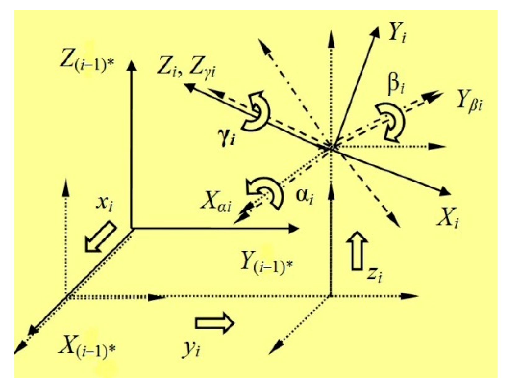
Coordinate transformations inside the i joint can be described with a corresponding matrix as a function of the generalized coordinates S_i

$$A_{(i-1)i}(S_i)=A_{(i-1)\alpha }(x_i,y_i,z_i)A_{\alpha \beta }({\alpha }_i)A_{\beta \gamma }({\beta }_i)A_{\gamma i}({\gamma }_i)$$

(3)

where A_(i-1)α—parallel translation matrix corresponding to generalized coordinates S_i reflecting linear deviations in the joint; A_αβ, A_βγ, and A_γi—rotation matrices by (α_i, β_i, γ_i) angles around the i link coordinate system axes. These rotation matrices reflect the angular deviations in the joint (Figure 2).

Equation (2) and Figure 2 show that the generalized angular coordinates should be considered as Euler angles. Since rotations by these angles are not commutative, the sequence of angular coordinates transformations must be specified.

3. Dynamic Model Development

Let us model manipulation systems with joints. We take the changing deviations into account. We can solve the equations of motion by numerical integration. The equations of action can be obtained by one of the theoretical mechanics’ methods, for example, the Lagrange–Euler method. The expression for the kinetic energy of the manipulation system as a rigid-body system is [5,6]:

$$E=\frac{1}{2}{\displaystyle \sum _{k=1}^n\mathrm{tr}({\dot{A}}_{0k}{H}_k{\dot{A}}_{0k}^{\mathrm{T}})}$$

(4)

where H_k—inertia matrix (4 × 4) for the k link considered as a rigid body.

Lagrange equation of the second kind combined with Expression (4), after transforming, gives the following equation:

$$\frac{d}{dt}\left(\frac{\partial E}{\partial s_{ij}}\right)-\frac{\partial E}{\partial s_{ij}}={\displaystyle \sum _{k=1}^n\mathrm{tr}\left(\frac{\partial A_{0k}}{\partial s_{ij}}{H}_k{\ddot{A}}_{0k}^{\mathrm{T}}\right)}$$

(5)

where tr(M)—M matrix diagonal elements’ sum.

The second derivative of the A_0k matrix gives the sum:

$$\begin{array}{ll}\hfill {\ddot{A}}_{0k}& ={\displaystyle \sum _{i=1}^n\left(\frac{\partial A_{0k}}{\partial x_i}{\ddot{x}}_i+\frac{\partial A_{0k}}{\partial y_i}{\ddot{y}}_i+\frac{\partial A_{0k}}{\partial z_{{}_i}}{\ddot{z}}_i+\frac{\partial A_{0k}}{\partial {\alpha }_i}{\ddot{\alpha }}_i+\frac{\partial A_{0k}}{\partial {\beta }_i}{\ddot{\beta }}_i+\frac{\partial A_{0k}}{\partial {\gamma }_i}{\ddot{\gamma }}_i\right)+}\\ & +{\displaystyle \sum _{i=1}^n{\displaystyle \sum _{j=1}^n\left(\begin{array}{l}\frac{{\partial }^2{A}_{0k}}{\partial {\alpha }_i\partial {\alpha }_j}{\dot{\alpha }}_i{\dot{\alpha }}_j+\frac{{\partial }^2{A}_{0k}}{\partial {\alpha }_i\partial {\beta }_j}{\dot{\alpha }}_i{\dot{\beta }}_j+\frac{{\partial }^2{A}_{0k}}{\partial {\alpha }_i\partial {\gamma }_j}{\dot{\alpha }}_i{\dot{\gamma }}_j+\\ +\frac{{\partial }^2{A}_{0k}}{\partial {\beta }_i\partial {\alpha }_j}{\dot{\beta }}_i{\dot{\alpha }}_j+\frac{{\partial }^2{A}_{0k}}{\partial {\beta }_i\partial {\beta }_j}{\dot{\beta }}_i{\dot{\beta }}_j+\frac{{\partial }^2{A}_{0k}}{\partial {\beta }_i\partial {\gamma }_j}{\dot{\beta }}_i{\dot{\gamma }}_j+\\ +\frac{{\partial }^2{A}_{0k}}{\partial {\gamma }_i\partial {\alpha }_j}{\dot{\gamma }}_i{\dot{\alpha }}_j+\frac{{\partial }^2{A}_{0k}}{\partial {\gamma }_i\partial {\beta }_j}{\dot{\gamma }}_i{\dot{\beta }}_j+\frac{{\partial }^2{A}_{0k}}{\partial {\gamma }_i\partial {\gamma }_j}{\dot{\gamma }}_i{\dot{\gamma }}_j\end{array}\right)}}+\\ & +{\displaystyle \sum _{i=1}^n{\displaystyle \sum _{j=1}^n\left(\begin{array}{l}\frac{{\partial }^2{A}_{0k}}{\partial {\alpha }_i\partial x_j}{\dot{\alpha }}_i{\dot{x}}_j+\frac{{\partial }^2{A}_{0k}}{\partial {\alpha }_i\partial y_j}{\dot{\alpha }}_i{\dot{y}}_j+\frac{{\partial }^2{A}_{0k}}{\partial {\alpha }_i\partial z_j}{\dot{\alpha }}_i{\dot{z}}_j+\\ +\frac{{\partial }^2{A}_{0k}}{\partial {\beta }_i\partial x_j}{\dot{\beta }}_i{\dot{x}}_j+\frac{{\partial }^2{A}_{0k}}{\partial {\beta }_i\partial y_j}{\dot{\beta }}_i{\dot{y}}_j+\frac{{\partial }^2{A}_{0k}}{\partial {\beta }_i\partial z_j}{\dot{\beta }}_i{\dot{z}}_j+\\ +\frac{{\partial }^2{A}_{0k}}{\partial {\gamma }_i\partial x_j}{\dot{\gamma }}_i{\dot{x}}_j+\frac{{\partial }^2{A}_{0k}}{\partial {\gamma }_i\partial y_j}{\dot{\gamma }}_i{\dot{y}}_j+\frac{{\partial }^2{A}_{0k}}{\partial {\gamma }_i\partial z_j}{\dot{\gamma }}_i{\dot{z}}_j\end{array}\right)}}+\\ & +{\displaystyle \sum _{i=1}^n{\displaystyle \sum _{j=1}^n\left(\begin{array}{l}+\frac{{\partial }^2{A}_{0k}}{\partial x_i\partial x_j}{\dot{x}}_i{\dot{x}}_j+\frac{{\partial }^2{A}_{0k}}{\partial x_i\partial y_j}{\dot{x}}_i{\dot{y}}_j+\frac{{\partial }^2{A}_{0k}}{\partial x_i\partial z_j}{\dot{x}}_i{\dot{z}}_j+\\ +\frac{{\partial }^2{A}_{0k}}{\partial y_i\partial x_j}{\dot{y}}_i{\dot{x}}_j+\frac{{\partial }^2{A}_{0k}}{\partial y_i\partial y_j}{\dot{y}}_i{\dot{y}}_j+\frac{{\partial }^2{A}_{0k}}{\partial y_i\partial z_j}{\dot{y}}_i{\dot{z}}_j+\\ +\frac{{\partial }^2{A}_{0k}}{\partial z_i\partial x_j}{\dot{z}}_i{\dot{x}}_j+\frac{{\partial }^2{A}_{0k}}{\partial z_i\partial y_j}{\dot{z}}_i{\dot{y}}_j+\frac{{\partial }^2{A}_{0k}}{\partial z_i\partial z_j}{\dot{z}}_i{\dot{z}}_j\end{array}\right)}}\end{array}$$

(6)

In Equation (6), the last block of terms is identically zero due to the property:

$$\frac{{\partial }^2{A}_{0k}}{\partial X_i\partial X_j}=0\left(i,j=1,\dots ,n\right)$$

(7)

where X_i = (x_i, y_i, z_i), X_j = (x_j, y_j, z_j). Let us prove it as a lemma.

Proof. 

The structure of the transformation matrix of homogeneous coordinates A_0k has the form (2). Since the relative rotation matrices R_0k are functions of only generalized angular coordinates Ω_i = [α_i β_i γ_i] (I = 1,…, n), and the expression can represent the vector X_0k

$$X_{0k}={\displaystyle \sum _{i=1}^k{R}_{(i-1)i}{X}_i}$$

(8)

then this vector is a function of both linear and angular coordinates X_0k = X_0k(X_i, Ω_i). Then, differentiating the matrix A_0k will give the matrix

$$\frac{\partial A_{0k}}{\partial X_i}=\left[\begin{array}{cc}\stackrel{3\times 3}{0}& \stackrel{3\times 3}{R_{(i-1)i}}\stackrel{3\times 1}{\left\{1\right\}}\\ 000& 0\end{array}\right]$$

(9)

where {1} = [1 1 1]^T is a vector (3 × 1).

Re-differentiating the matrix A_0k will give a null matrix. Thus, the lemma corresponding to property (7) is proved.

Property (7) reflects the absence of Coriolis and centrifugal accelerations when considering the relative motion of translationally moving coordinate systems.

Expression (6), taking into account property (7), is substituted into Equation (5).

Having grouped the terms and separated the vectors of velocities and accelerations of the generalized coordinates, we represent the equations of motion in matrix form for each generalized force corresponding to one of the generalized coordinates.

$$\begin{array}{c}{M}_i^{sx}\ddot{x}+M_i^{sy}\ddot{y}+M_i^{sz}\ddot{z}+\\ M_i^{s\alpha }\ddot{\mathsf{\alpha }}+M_i^{s\beta }\ddot{\mathsf{\beta }}+M_i^{s\gamma }\ddot{\mathsf{\gamma }}+\\ +{\dot{\mathsf{\alpha }}}^{\mathrm{T}}{C}_i^{s\alpha \alpha }\dot{\mathsf{\alpha }}+{\dot{\mathsf{\beta }}}^{\mathrm{T}}{C}_i^{s\beta \beta }\dot{\mathsf{\beta }}+{\dot{\mathsf{\gamma }}}^{\mathrm{T}}{C}_i^{s\gamma \gamma }\dot{\mathsf{\gamma }}+\\ +2\left({\dot{\mathsf{\alpha }}}^{\mathrm{T}}{C}_i^{s\alpha \beta }\dot{\mathsf{\beta }}+{\dot{\mathsf{\alpha }}}^{\mathrm{T}}{C}_i^{s\alpha \gamma }\dot{\mathsf{\gamma }}+{\dot{\mathsf{\beta }}}^{\mathrm{T}}{C}_i^{s\beta \gamma }\dot{\mathsf{\gamma }}\right)+\\ +2\left({\dot{\mathsf{x}}}^{\mathrm{T}}{C}_i^{sx\alpha }\dot{\mathsf{\alpha }}+{\dot{\mathbf{x}}}^{\mathrm{T}}{C}_i^{sx\beta }\dot{\mathsf{\beta }}+{\dot{x}}^{\mathrm{T}}{C}_i^{sx\gamma }\dot{\mathsf{\gamma }}\right)+\\ +2\left({\dot{y}}^{\mathrm{T}}{C}_i^{sy\alpha }\dot{\mathsf{\alpha }}+{\dot{y}}^{\mathrm{T}}{C}_i^{sy\beta }\dot{\mathsf{\beta }}+{\dot{y}}^{\mathrm{T}}{C}_i^{sy\gamma }\dot{\mathsf{\gamma }}\right)+\\ +2\left({\dot{z}}^{\mathrm{T}}{C}_i^{sz\alpha }\dot{\mathsf{\alpha }}+{\dot{z}}^{\mathrm{T}}{C}_i^{sz\beta }\dot{\mathsf{\beta }}+{\dot{z}}^{\mathrm{T}}{C}_i^{sz\gamma }\dot{\mathsf{\gamma }}\right)=Q_i^s\end{array}$$

(10)

where M and C—matrices (1 × n) и (n × n), respectively; $\dot{x}$, $\ddot{x}$, $\dot{y}$, $\ddot{y}$, $\dot{z}$, $\ddot{z}$, $\dot{\mathsf{\alpha }}$, $\ddot{\mathsf{\alpha }}$, $\dot{\mathsf{\beta }}$, $\ddot{\mathsf{\beta }}$, $\dot{\mathsf{\gamma }}$, $\ddot{\mathsf{\gamma }}$—vectors (n × 1) of velocities and accelerations of the corresponding generalized coordinates;$Q_i^s$– generalized force (scalar) corresponding to one of the generalized coordinates S_i = [s_ij], (I = 1,…, n; j = 1,…, 6).

4. Dynamic Model Analysis

The matrix coefficients of the obtained equations can be presented in expanded form. Symbols s, v, and w were used to symbolize the indices corresponding to the generalized coordinates S_i = [s_ij] = [X_i, Ω_i]:

$$M_i^{sv}={\displaystyle \sum _{k=1}^n\left[\begin{array}{cccc}\mathrm{tr}\left(\frac{\partial A_{0k}}{\partial s_{ij}}{H}_k\frac{\partial A_k^{\mathrm{T}}}{\partial v_1}\right)& \mathrm{tr}\left(\frac{\partial A_{0k}}{\partial s_{ij}}{H}_k\frac{\partial A_{0k}^{\mathrm{T}}}{\partial v_2}\right)& \dots & \mathrm{tr}\left(\frac{\partial A_{0k}}{\partial s_{ij}}{H}_k\frac{\partial A_{0k}^{\mathrm{T}}}{\partial v_n}\right)\end{array}\right]}$$

(11)

$$C_i^{svw}={\displaystyle \sum _{k=1}^n\left[\begin{array}{cccc}\mathrm{tr}\left(\frac{\partial A_{0k}}{\partial s_{ij}}{H}_k\frac{{\partial }^2{A}_{0k}^{\mathrm{T}}}{\partial v_1\partial w_1}\right)& \mathrm{tr}\left(\frac{\partial A_{0k}}{\partial s_{ij}}{H}_k\frac{{\partial }^2{A}_{0k}^{\mathrm{T}}}{\partial v_1\partial w_2}\right)& \dots & \mathrm{tr}\left(\frac{\partial A_{0k}}{\partial s_{ij}}{H}_k\frac{{\partial }^2{A}_{0k}^{\mathrm{T}}}{\partial v_1\partial w_n}\right)\\ \mathrm{tr}\left(\frac{\partial A_{0k}}{\partial s_{ij}}{H}_k\frac{{\partial }^2{A}_{0k}^{\mathrm{T}}}{\partial v_2\partial w_1}\right)& \mathrm{tr}\left(\frac{\partial A_{0k}}{\partial s_{ij}}{H}_k\frac{{\partial }^2{A}_{0k}^{\mathrm{T}}}{\partial v_2\partial w_2}\right)& \dots & \mathrm{tr}\left(\frac{\partial A_{0k}}{\partial s_{ij}}{H}_k\frac{{\partial }^2{A}_{0k}^{\mathrm{T}}}{\partial v_2\partial w_n}\right)\\ \dots & \dots & \dots & \dots \\ \mathrm{tr}\left(\frac{\partial A_{0k}}{\partial s_{ij}}{H}_k\frac{{\partial }^2{A}_{0k}^{\mathrm{T}}}{\partial v_n\partial w_1}\right)& \mathrm{tr}\left(\frac{\partial A_{0k}}{\partial s_{ij}}{H}_k\frac{{\partial }^2{A}_{0k}^{\mathrm{T}}}{\partial v_n\partial w_2}\right)& \dots & \mathrm{tr}\left(\frac{\partial A_{0k}}{\partial s_{ij}}{H}_k\frac{{\partial }^2{A}_{0k}^{\mathrm{T}}}{\partial v_n\partial w_n}\right)\end{array}\right]}$$

(12)

So, for example, for the equation corresponding to the generalized coordinate s₁₁ (equals x₁ in $M_i^{sv}$ notation) for the first matrix in Equation (10), i = 1, and both s and v match x. The sixth matrix, s, also matches x, and v matches γ. In $C_i^{svw}$ notation, for a given generalized coordinate, the symbol s corresponds to x, and the symbols v and w correspond to the indices that determine the position of this matrix in Equation (10).

Row matrices $M_i^{sv}$ have the dimension 1 × n. These matrices elements defined by the expressions $\mathrm{tr}\left(\frac{\partial A_{0k}}{\partial s_{ij}}{H}_k\frac{\partial A_{0k}^{\mathrm{T}}}{\partial v_l}\right)$ (i, l, k = 1, …, n; j = 1, …, 6) turn to zero in case $i>k$ or $l>k$. However, the analyzed row matrices represent the sums $M_i^{sv}={\displaystyle \sum _{k=1}^n{M}_{ki}^{sv}}$. So, as a result, their elements will be nonzero.

Analysis of $C_i^{svw}$ matrices of n × n dimension also shows that, in the general case, their elements are not equal to zero. The elements of these matrices defined by the expressions $\mathrm{tr}\left(\frac{\partial A_{0k}}{\partial s_{ij}}{H}_k\frac{{\partial }^2{A}_{0k}^{\mathrm{T}}}{\partial v_l\partial w_f}\right)$ (i, l, f, k = 1, ..., n; j = 1, ..., 6) turn to zero if $i>k$, or $l>k$, or $f>k$. In addition, these elements also turn to zero for some kinematic schemes due to the absence of centrifugal and/or Coriolis forces.

Thus, the obtained Equation (10) is the desired equation of motion. Moreover, the equation makes it possible to consider the deviations rising in the joints of manipulation robots, considered as generalized coordinates S_i = [s_ij].

Thus, the obtained Equation (10) is the desired equation of motion. Moreover, it makes it possible to consider the deviations arising in the joints of manipulation robots, considered as generalized coordinates S_i = [s_ij].

5. Generalized Forces

The right sides of the obtained equations represent the generalized forces in the i joint along the corresponding generalized coordinate. The potential energy was not reflected on the left side of the Lagrange equation of the second kind (4). Thus, its influence should be taken into account on the right side of the equation of motion. If the generalized coordinate corresponds to elastic deformations, then the generalized force can be given by the expression:

$$Q_{Pi}^s=-a_i^s{s}_{ij}-b_i^s{\dot{s}}_{ij}$$

(13)

where $a_i^s$ and $b_i^s$—the stiffness and viscosity coefficients of the i joint along the s_ij generalized coordinate direction.

The expression for generalized forces corresponding to the external forces represented by the principal vector and the principal moment applied to the centers of gravity of the links has the form [5]:

$$Q_{Fi}^s={\displaystyle \sum _{k=i}^n\left(F_{0k}^{\mathrm{T}}\frac{\partial A_{0k}}{\partial s_{ij}}{r}_C^{(k)}+R_{0k}^{\mathrm{T}}{A}_{0i}{\mathsf{\Theta }}_i\right)}$$

(14)

where $F_{0k}={\left[\begin{array}{cccc}{F}_{kx}& F_{ky}& F_{kz}& 0\end{array}\right]}^{\mathrm{T}}$—principal vector, and $R_{0k}={\left[\begin{array}{cccc}{R}_{kx}& R_{ky}& R_{kz}& 0\end{array}\right]}^{\mathrm{T}}$—principal moment of external forces acting on the k link given in a fixed-coordinate system O₀; $r_C^{(k)}$—center of the gravity radius vector of the k link, selected for the reference point of external forces; ${\mathsf{\Theta }}_i={\left[\begin{array}{cccc}0& 0& {\theta }_i& 0\end{array}\right]}^{\mathrm{T}}$—auxiliary vector; θ_i = 1, if I hinge is a rotational one, and θ_i = 0, if i hinge is a translational one.

Equation (14) can also take into account the influence of gravity forces on the links, as these forces can be considered similarly to the principal vector of external forces.

Consider the most common case of representing the right side of the equations of motion for manipulation robots. This takes into account the generalized forces from the external forces’ action corresponding to the principal vector and the principal moment at the center of gravity of the links, the gravity forces of the links and the manipulation object, the forces developed by the drives, and the elastic forces and resistance forces arising in the joints.

$$Q_i^s=Q_{Pi}^s+Q_{Fi}^s+Q_{Gi}^s+Q_{Di}^s$$

(15)

where $Q_{Pi}^s$—elastic forces and resistance forces arising in the joints—see Equation (13); $Q_{Fi}^s$—generalized forces from external forces—see Equation (14); $Q_{Gi}^s$—generalized forces from gravity—see Equation (14); $Q_{Di}^s$—generalized forces from the forces developed by the drives.

Generalized forces $Q_{Di}^s$ corresponding to forces (moments of forces) by the drives D_ij, (i = 1,…, n; j = 1,…, 6) are equal to these forces. Since the elementary work of the drives on possible displacements is the following sum:

$$\partial W_D={\displaystyle \sum _{i=1}^n{\displaystyle \sum _{j=1}^6{D}_{ij}\delta s_{ij}}}$$

(16)

therefore, in accordance with the definition of generalized forces, $Q_{Di}^s=D_{ij}$.

6. Verification

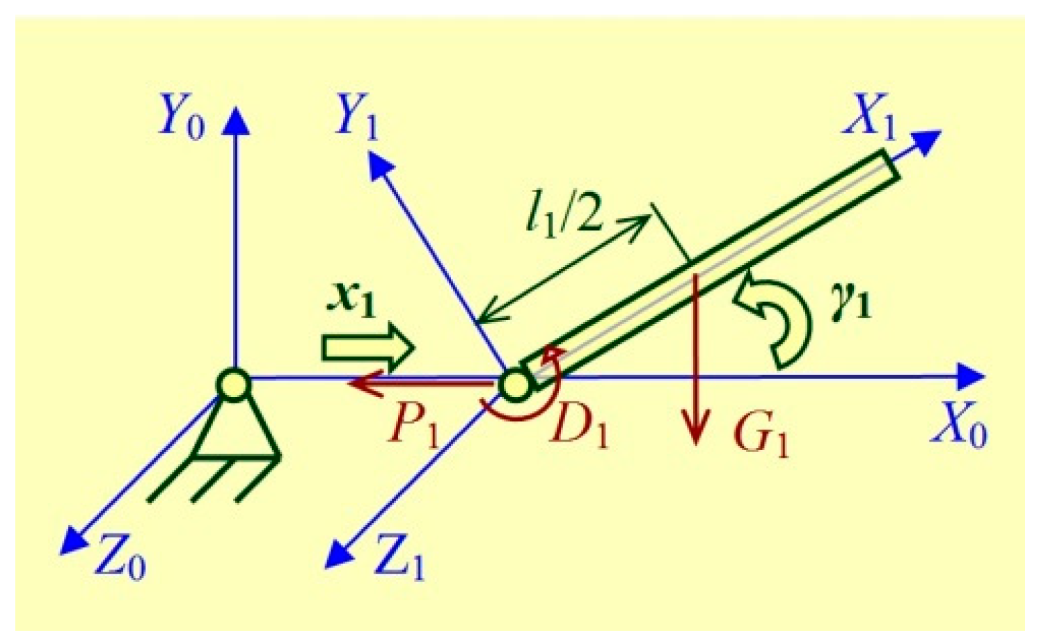
Let us consider the application of the obtained equations of motion using the example of a manipulation robot with one link connected to a fixed base by a rotary joint (Figure 3). The investigated manipulation system has two degrees of freedom; one is the main rotational one—γ₁—corresponding to the constructive mobility of the joint; the second is translational one—x₁—due to the malleability of the joint along the X₀ axis. The link is a rod of length l₁ and mass m₁. Active forces acting on the link are the torque D₁ developed by the drive, the link gravity G₁ = m₁g (g = 9.81 m/c²) and elastic force P₁ = −a₁x₁ arising in the joint during its deformation along X₀ axis, and joint stiffness in that direction.

$$M_1^{xx}{\ddot{x}}_1+M_1^{x\gamma }{\ddot{\gamma }}_1+C_1^{x\gamma \gamma }{\dot{\gamma }}_1^2+2{\dot{x}}_1{C}_1^{xx\gamma }{\dot{\gamma }}_1=Q_1^x$$

(17)

$$M_1^{\gamma \gamma }{\ddot{\gamma }}_1+M_1^{\gamma x}{\ddot{x}}_1+C_1^{\gamma \gamma \gamma }{\dot{\gamma }}_1^2+2{\dot{x}}_1{C}_1^{\gamma x\gamma }{\dot{\gamma }}_1=Q_1^{\gamma }$$

(18)

The matrix coefficients in Equations (17) and (18), obtained with (11) and (12), can be reduced to scalar form:

$$\begin{array}{c}{M}_1^{xx}=\mathrm{tr}\left(\frac{\partial A_{01}}{\partial x_1}{H}_1\frac{\partial A_{01}^{\mathrm{T}}}{\partial x_1}\right), M_1^{x\gamma }=\mathrm{tr}\left(\frac{\partial A_{01}}{\partial x_1}{H}_1\frac{\partial A_{01}^{\mathrm{T}}}{\partial {\gamma }_1}\right),\\ M_1^{\gamma \gamma }=\mathrm{tr}\left(\frac{\partial A_{01}}{\partial {\gamma }_1}{H}_1\frac{\partial A_{01}^{\mathrm{T}}}{\partial {\gamma }_1}\right),M_1^{\gamma x}=\mathrm{tr}\left(\frac{\partial A_{01}}{\partial {\gamma }_1}{H}_1\frac{\partial A_{01}^{\mathrm{T}}}{\partial x_1}\right),\\ C_1^{x\gamma \gamma }=\mathrm{tr}\left(\frac{\partial A_{01}}{\partial x_1}{H}_1\frac{{\partial }^2{A}_{01}^{\mathrm{T}}}{\partial {\gamma }_1^2}\right),C_1^{xx\gamma }=\mathrm{tr}\left(\frac{\partial A_{01}}{\partial x_1}{H}_1\frac{{\partial }^2{A}_{01}^{\mathrm{T}}}{\partial x_1\partial {\gamma }_1}\right),\\ C_1^{\gamma x\gamma }=\mathrm{tr}\left(\frac{\partial A_{01}}{\partial {\gamma }_1}{H}_1\frac{{\partial }^2{A}_{01}^{\mathrm{T}}}{\partial x_1\partial {\gamma }_1}\right).\end{array}$$

Conversion matrices of homogeneous coordinates and their partial derivatives for the studied manipulation system have the form:

$$\begin{array}{c}{A}_{01}=\left[\begin{array}{cccc}\cos {\gamma }_1& -\sin {\gamma }_1& 0& x_1\\ \sin {\gamma }_1& \cos {\gamma }_1& 0& 0\\ 0& 0& 1& 0\\ 0& 0& 0& 1\end{array}\right],\frac{\partial A_{01}}{\partial x_1}=\left[\begin{array}{cccc}0& 0& 0& 1\\ 0& 0& 0& 0\\ 0& 0& 0& 0\\ 0& 0& 0& 0\end{array}\right],\\ \frac{\partial A_{01}}{\partial {\gamma }_1}=\left[\begin{array}{cccc}-\sin {\gamma }_1& -\cos {\gamma }_1& 0& 0\\ \cos {\gamma }_1& -\sin {\gamma }_1& 0& 0\\ 0& 0& 0& 0\\ 0& 0& 0& 0\end{array}\right],\\ \frac{{\partial }^2{A}_{01}}{\partial {\gamma }_1^2}=\left[\begin{array}{cccc}-\cos {\gamma }_1& \sin {\gamma }_1& 0& 0\\ -\sin {\gamma }_1& -\cos {\gamma }_1& 0& 0\\ 0& 0& 0& 0\\ 0& 0& 0& 0\end{array}\right],\frac{{\partial }^2{A}_{01}}{\partial {\gamma }_1\partial x_1}=0.\end{array}$$

The inertia matrix of the link relative to the coordinate system S₁ (X₁, Y₁, Z₁), in accordance with the transformation rule for inertia matrices [6], has the following form:

$$H_1=\left[\begin{array}{cccc}1& 0& 0& \frac{l_1}{2}\\ 0& 1& 0& 0\\ 0& 0& 1& 0\\ 0& 0& 0& 1\end{array}\right]\left[\begin{array}{cccc}\frac{m_1{l}_1^2}{12}& 0& 0& 0\\ 0& 0& 0& 0\\ 0& 0& 0& 0\\ 0& 0& 0& m_1\end{array}\right]\left[\begin{array}{cccc}1& 0& 0& 0\\ 0& 1& 0& 0\\ 0& 0& 1& 0\\ \frac{l_1}{2}& 0& 0& 1\end{array}\right]=\left[\begin{array}{cccc}\frac{m_1{l}_1^2}{3}& 0& 0& \frac{m_1{l}_1}{2}\\ 0& 0& 0& 0\\ 0& 0& 0& 0\\ \frac{m_1{l}_1}{2}& 0& 0& m_1\end{array}\right]$$

Using the obtained matrices in expressions for the corresponding matrix coefficients, we obtain the expressions:

$$\begin{array}{c}{M}_1^{xx}=m_1, M_1^{x\gamma }=-\frac{m_1{l}_1}{2}\sin {\gamma }_1, M_1^{\gamma \gamma }=\frac{m_1{l}_1^2}{3},M_1^{\gamma x}=-\frac{m_1{l}_1}{2}\sin {\gamma }_1,\\ C_1^{x\gamma \gamma }=-\frac{m_1{l}_1}{2}\cos {\gamma }_1, C_1^{xx\gamma }=0,C_1^{\gamma \gamma \gamma }=0, C_1^{\gamma x\gamma }=0.\end{array}$$

Substituting the obtained expressions for the matrix coefficients, and the generalized forces obtained in accordance with (13)–(16), into Equations (17) and (18), we compose a system of differential equations.

$$\{\begin{array}{l}{m}_1{\ddot{x}}_1-\frac{m_1{l}_1\sin {\gamma }_1}{2}{\ddot{\gamma }}_1-\frac{m_1{l}_1\cos {\gamma }_1}{2}{\dot{\gamma }}_1^2=-a_1{x}_1\\ \frac{m_1{l}_1^2}{3}{\ddot{\gamma }}_1-\frac{m_1{l}_1\sin {\gamma }_1}{2}{\ddot{x}}_1=D_1-\frac{1}{2}{l}_1{m}_{1}g\sin {\gamma }_1\end{array}$$

(19)

The system of Equation (19) compiled based on (10) correctly describes the movement of the investigated manipulation robot, considered as a rigid body, performing both translational and rotational actions (Figure 3). Other known methods of theoretical mechanics can also obtain these equations.

7. Discussion

The presented mathematical model (dynamic model) (10)–(15) is obtained on the basis of strict transformations of the equations of motion compiled on the basis of the Lagrange–Euler method, well known in theoretical mechanics. In the initial equations, elements identically equal to zero were excluded. This became possible on the basis of the proved lemma (6); the proof is not given in this article. Operations with zero elements of matrices (4 × 4) transformations of homogeneous coordinates were also excluded.

The exclusion of elements identically equal to zero from the equations significantly increased the computational efficiency of the mathematical model. As is known, the computational complexity of the equations of motion obtained based on the Lagrange-Euler method is proportional to the square of the number of generalized coordinates (n²). In contrast, the Newton–Euler method gives a linear dependence. Therefore, until now, when modeling the movement of manipulative robots in real-time, the Newton–Euler method is mainly used. The developed algorithm makes it possible to bring both methods closer in terms of their computational efficiency.

The correctness of the obtained equations was confirmed analytically using the example of a 2-DOF robot. For systems with a large number of degrees of freedom, it is necessary to use computer calculations. Such comparative analyses were carried out during verification of the developed method, but not for the effectiveness of algorithms but the accuracy of estimates. The trajectories of the characteristic point (TCP—tool center point) of the 6-DOF robot, constructed in one of the well-known CAD systems and obtained based on the developed method, were compared. The result of the experiment was a complete coincidence of the calculated trajectories.

The developed method can be used to model mechanical systems with many degrees of freedom—for example, anthropomorphic robots. There are no fundamental restrictions for this. The algorithm implementing calculations by this method allocates the required amount of memory dynamically and allows modeling open kinematic structures with unlimited degrees of freedom. Any closed kinematic systems can be brought to an empty form by conditionally cutting the joints. At the same time, additional equations of connections and external forces corresponding to reactions in “cut” joints will need to be added to the mathematical model. Furthermore, the algorithm allows joints with different mobilities (1–6)-DOF.

The main advantage of the method presented in the article is that, in addition to the exact calculation of program trajectories, it allows calculating all possible deviations from a given motion. The reason for such variations may be elastic flexibility in the joints; therefore, 6-DOF joints are used in our model. Unfortunately, this leads to the fact that in order to simulate a 6-DOF robot with 6-DOF joints, you need to compose not six but thirty-six equations of motion. Therefore, when we conducted a test for the accuracy of constructing the trajectory of a 6-DOF robot, the capabilities of our algorithm were only used by 1/6.

In contrast to the Lagrange–Euler method, an additional advantage of the developed method is the possibility inherent in it to determine the reactions in the joints of the robot necessary to perform the specified movements. The method makes it possible to calculate projections of forces and moments of support reactions in three-dimensional space with a decrease in joint mobility. This makes it possible to search for the optimal kinematic structure of the robot for solving special tasks.

8. Conclusions

A dynamic model based on matrix differential equations describing the movements of manipulative robots is obtained. The kinematic structure of the simulated robots described by these equations allows joints to have six degrees of freedom (6-DOF Joints).

We considered the links of the manipulation system as solid bodies. Therefore, when composing the coefficient matrices of these equations, we excluded elements that are also equal to zero. This significantly reduced the number of calculations. The excluded elements reflect the mutual influence of the degrees of mobility responsible for linear orthogonal displacements in the joints.

This dynamic model makes it possible to analyze the movements of manipulative robots, taking into account the deviations that occur in their joints—for example, due to elastic deformations or ruptures. Using computer modeling allows for a comprehensive analysis of the dynamics of simulation robots with an unlimited number of degrees of freedom.

Additionally, this dynamic model can be used to analyze deviations in the tasks of stabilizing the position of manipulation systems installed on non-rigidly stabilized platforms, for example, quadrocopters [22,23,24]. At the same time, parametric perturbations of the platform should be considered as deviations in the 6-DOF joint connecting the manipulating robot to the platform.

The harvesting robot developed at the Financial University (Moscow) for apple crops will be equipped with a multi-link manipulation system [38]. The results presented in the article will help improve this manipulative robot’s work and demonstrate the importance of the developed mathematical models for real practical applications.