Multicriteria Optimization of a Dynamic System by Methods of the Theories of Similarity and Criteria Importance

Abstract

The problem of multicriteria optimization of a dynamic model is solved using the methods of the similarity theory and the criteria importance theory. The authors propose the original model of a positional system with two hydraulic actuators, synchronously moving a heavy object with a given accuracy. In order to reduce the number of optimizing parameters, the mathematical model of the system is presented in a dimensionless form. Three dimensionless optimization criteria that characterize the accuracy, size, and quality of the dynamic positioning process are considered. It is shown that the application of the criteria importance method significantly reduces the Pareto set (the set of the best solutions). This opens up the possibility of reducing many optimal solutions to one solution, which greatly facilitates the choice of parameters when designing a mechanical object.

1. Introduction

Artificial intelligence is now widely used in industry, applied to transporting mechanisms, such as robots and manipulators, which move and deliver various objects to specified positions. In simple loading systems, the accuracy of moving and positioning of goods can be relatively low, which makes it possible to use relatively simple devices in these cases. However, feeding a tool in processing machines requires a sufficiently high accuracy. The movement of robots can be carried out by various actuators: pneumatic, hydraulic, electric, etc.

Positioning control problems in transporting mechanisms (robots) are solved mainly in two ways: using special type regulators, such as based on fuzzy logic, neural networks, and so on or the ordinary regulators with feedback control of various type. The mathematical models of actuators, as a rule, have a rather complex structure, consisting of higher-order differential and algebraic equations.

Developing new devices requires the solving of a number of technical problems associated with the choice of their type, structure, and control system, satisfied to many requirements. In mechanical systems, hydraulic actuators are widely used. Their main advantage in relation to pneumatic and electric actuators is their high carrying capacity and low sensitivity to the load variation [1].

Mathematical models of hydraulic actuators and their control systems are well studied and fully presented in works, such as [2,3,4,5]. However, the problem of finding the best constructive solution in most cases is based of the original models not reduced to a dimensionless form. Due to the abundance of differently sized variables, the general patterns of the results obtained are often not visible, it is difficult to single out the groups of criteria to be optimized. Additionally, it is not advisable to optimize un-grouped parameters (variables) at the same time. This was noted by example in [6].

In [7], the authors turn to dimensionless models, but do not use them systematically in the search for the best solution. In this case, the dimensionless model serves only to partially simplify the general formulation of the problem and to study the properties of the original model. The transition to dimensionless parameters was used to select a special object positioning control system, which should provide an approach to a given position simultaneously with zero speed and zero acceleration in order to avoid damage to the contact point when stopping.

The principle and process of transition to dimensionless forms have been developed for a long time. Here we can note the fundamental works in this area [8,9]. The importance of the theory of similarity and analogy in understanding the essence of things was noted back in the days of Plato. In a number of philosophical works, attempts have been made to generalize approaches to equivalence in different fields of knowledge, which gives this direction additional significance. In [10], a general metric of transition to dimensionless variables was considered and introduced, but it was noted that there is no uniquely best measure of dynamic similarity, since the feasibility of any given measure depends on its intended use.

In [11], it is shown that, due to the complexity of the mathematical description of technical dynamic systems, when choosing their structure and parameters, they usually turn to very laborious interactive (dialogue) procedures. A number of tools help to avoid direct enumeration of options when using such procedures, among which the methods of dimension and similarity theory take a significant place. These methods are based on the use of dimensionless complexes of physical parameters of the system (criteria of similarity and the relationship between them) together with the translation of the mathematical description of the system into a dimensionless form [12,13]. As a result, additional opportunities open up for identifying general patterns of dynamic processes, which greatly facilitates making the final decision.

Experience shows that each specific problem of the dynamics of a mechanical system requires a special approach to the formation of a dimensionless model and similarity criteria. The structure and form of the dimensionless model depends on the accepted units of measurement of the variables included in the equations of the model, and on the expressions attached to its coefficients. These factors are initially unknown and are usually formed according to the intuition and experience of the researcher, which introduces uncertainty in the process of transition to a dimensionless model and does not guarantee high efficiency of its use. The approach proposed below to the formation of dimensionless models of a dynamic system of a hydraulic actuator is a development of the procedure started in [11].

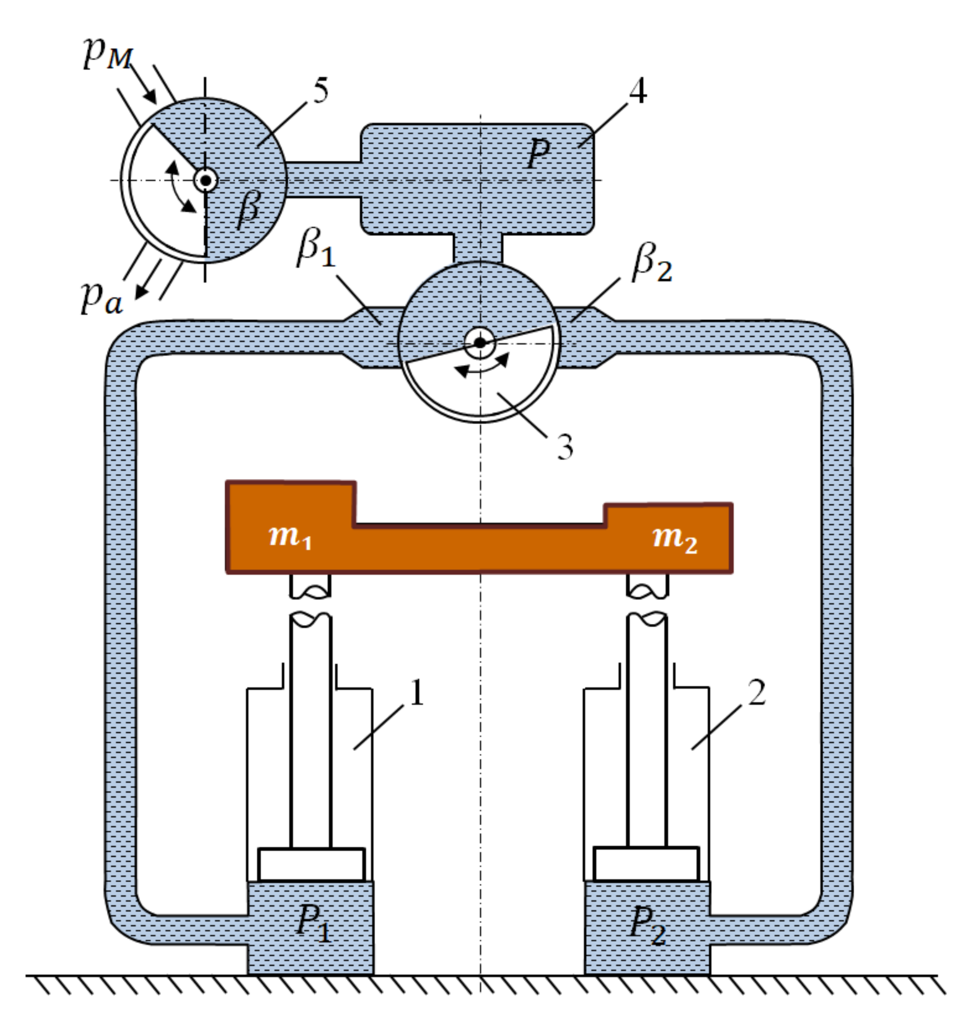
This paper illustrates an example of finding the optimal solution for a positional system with two hydraulic actuators. This type of actuator was chosen based on the task of controlled movement of a heavy and bulky object (load). The hydraulic actuator has the highest power density. However, the presence of two actuators creates special problems in control, since the drives must operate in coordination in both position and speed. Based on this, the authors proposed an original control scheme that solves this problem based on the use of only two valves (Figure 1): one of them regulates the average speed of the moving object, and the other controls the distribution of fluid flows directed into the cavities of the hydraulic cylinders [14,15].

The study of the mathematical model is carried out in dimensionless parameters, the transition to which hydraulic actuator systems are presented in [6]. Parametric synthesis is carried out according to the principle of multicriteria optimization. During the transition of the system to a dimensionless form, three optimization criteria are identified with further application of the criteria importance method. The criteria importance method significantly reduces the optimal solutions of the system, which facilitates the selection of the best solution when designing a mechanical object.

The parametric synthesis of a mechanical system consists in choosing the values of the parameters that make up the vector $X=(x_1,x_2,\dots ,x_n)$ that provide the best values of the characteristics (performance indicators) of the system that make up the vector $K=(k_1,k_2,\dots ,k_m)$. Thus, the problem of multicriteria (multi-objective) optimization is posed, in which X is a vector of variables, and $K\left(X\right)$ is a vector of criteria (objective functions).

To solve this problem, it is necessary to develop an adequate mathematical model of the system under consideration, using the vector X as input parameters and calculating the values of the characteristics $K\left(X\right)$ at the output. Further, it is necessary to implement a method for solving the optimization problem. In addition, in the presence of several characteristics ($m>1$), it is required to take into account the dependencies and preferences between them.

Complex mechanical systems usually contain up to several tens of parameters n and several characteristics m. At the same time, mathematical models of dynamic systems contain complex connections and differential equations, and for calculations they require the use of numerical methods. Therefore, when solving the problem of optimizing such complex systems, the computational model usually represents a “black box”, which makes it practically impossible to use local, gradient optimization methods [16,17]. Among the global optimization methods working with such complex models, genetic algorithms [18], and other variations of evolutionary algorithms, particle swarm optimization [19], and simulated annealing methods [20]. In this paper, for the global search for optimal solutions, the parameter space investigation method [21] is used, based on the construction of sequences of points uniformly distributed in the feasible area of the parameters X space [22].

In multicriteria optimization problems, as a rule, it is not possible to obtain a feasible solution that is best at once according to all criteria. Using formal mathematical and numerical methods, a set of Pareto optimal solutions can be obtained (approximated). To select the one best solution among them, it is necessary to involve additional information about the preferences regarding these criteria.

There are a priori and a posteriori methods for solving multicriteria optimization problems. In a priori methods, the question of preferences is resolved before the search for solutions is carried out. These methods include the method of identifying the “main” criterion, as well as various methods of convolution of the criteria into one aggregated performance indicator. For example, the weighted sum $F_{\sum }\left(X\right)={\sum }_{i=1}^m{w}_i{k}_i\left(X\right)$, the product $F_{\prod }\left(X\right)={\prod }_{i=1}^m{k}_i^{w_1}\left(X\right)$, or the Germeier convolution $F_G\left(X\right)=mi{n}_i{k}_i\left(X\right)/w_i$. Before convoluting, the criteria $k_i$ are normalized in a special way. This approach allows one to go straight to solving the optimization problem with one objective function. However, there are a number of disadvantages behind the simplicity of this approach. First of all, it is difficult for a person, no matter how expert he or she is, to set the exact values of the weights reflecting the relative importance of the criteria. In addition, there are a number of theoretical problems associated with the justification of this approach [23].

On the contrary, in a posteriori methods, optimization is performed first taking into account all the criteria, and then preferences are analyzed. Analysis of the set of obtained solutions is itself useful in solving such problems. First of all, a person, an expert working with such data of optimization results, understands the possibilities available to him or her: evaluates the areas of feasible solutions, the ranges of change in the values of the criteria. In such an analysis, visualization tools [24], and interactive interaction of an expert with a computer analytical system [25] play an important role. The more adequately the expert’s real preferences are revealed, the better the solution obtained on their basis will be. The preferences are most accurately established in the process of dialogue with the analytical system, during which a person sees intermediate solutions, obtains a clearer idea of the real conditions of the problem, resource opportunities, and goals. One of the most important properties of such systems is the ability to provide explanations (justifications) of the results and conclusions obtained, interpreting them in terms of the subject area, in a language understandable for an expert [26].

It is known that the best solution should be chosen among the set of Pareto optimal ones. However, this set of solutions is usually quite large. To narrow the scope of choice, additional assumptions should be made about the preferences of experts regarding the importance and values of the criteria. For formal modeling of these preferences and obtaining conclusions on the basis of this information, the approach of the mathematical theory of criteria importance was used in this work [27,28]. This method assumes a consistent refinement of information about preferences. First, the simplest information about ordering criteria by importance is found out. Such qualitative information is easier to obtain than quantitative estimates of importance, and, therefore, more reliably describes the expert’s real preferences. Next, the formal methods of the theory come into play, which make it possible to reasonably discard from consideration some of the solutions from the Pareto set, thereby narrowing the set of choices for the best solution. Then, if necessary, quantitative estimates of importance are also used, but not accurate, just in the form of intervals. Additionally, additional information about changing preferences along the criteria scale can be used.

2. Statement of the Problem and Mathematical Model of the System

The object of research in this work is a rather complex manipulator designed to lift a heavy, bulky load using two parallel and synchronously operating hydraulic actuators 1 and 2 (Figure 1). Let us describe the mathematical model of the object. The moving object has a mass $m=m_1+m_2$, where $m_{1,2}$ are the mass loads applied to the actuators. The main working cavities are the lower cavities of the actuators; however, if necessary, the upper cavities can also be used (for example, when lowering an object). The law of motion is mainly determined by the pressures in the lower cavities, which are connected through the control valve 3, the intermediate cavity 4 (volume V) and the control valve 5 when the object is lifted to the power source (with pressure $p_M$), and when the object is lowered, to the drain line (with pressure $p_A$, usually equal to atmospheric). The ratios between the effective flow area of the valve 5 and the effective flow areas of the valve channels 3 leading to the cavities of the actuators are established depending on the formulation of the problem.

The equations of movement are:

$$\begin{array}{c}{m}_i{\ddot{x}}_i=p_{i}F+m_{i}g{k}_i{\dot{x}}_i+P_{Li},i=1,2;\end{array}$$

(1)

where x is the piston displacement; $p_i$ are pressures in the lower cavities; F is the effective piston area; $m_{i}g$, $P_{Li}$ are weight and force load on the rod, respectively; $k_i$ are coefficients of fluid friction in the actuator.

The changes of the pressure $p_i$ in the lower cavities of the actuators and the pressure p in the intermediate cavity are related by dependencies:

$$\begin{array}{c}\dot{p}=W\left(\beta sign(\Delta p)\sqrt{|\Delta p|}-{\beta }_1{\alpha }_{1}sign(\Delta p_1)\sqrt{|\Delta p_1|}-{\beta }_2{\alpha }_{2}sign(\Delta p_2)\sqrt{|\Delta p_2|}\right),\\ \dot{p_i}=W_i\left({\beta }_i{\alpha }_{i}sign(\Delta p_i)\sqrt{|\Delta p_i|}-\dot{x_i}\right),\end{array}$$

(2)

where $W=\left(\frac{Ef}{F{x}_v}\right)\sqrt{\frac{2p_M}{\rho }}$, $W_i=\left(\frac{Ef}{F(x_{0i}+x_i)}\right)\sqrt{\frac{2p_M}{\rho }}$; $\Delta p=p_M-p$ (when lifting) or $\Delta p=p_A-p$ (when lowering) of the object, $\Delta p_i=p-p_i$; $\beta$, ${\beta }_1$ and ${\beta }_2$ are channel opening degrees f, $f_1$ and $f_2$; E is the bulk modulus of the working fluid; $x_v$ is the length of the intermediate cavity; $\rho$ is working fluid density.

3. Transformation of the Model into a Dimensionless Form

According to the method of the similarity theory [8] Equations (1) and (2) are transformed into a dimensionless form by replacing variables with their dimensionless analogs $\lambda$, $\tau$, $\sigma$, according to the relations $x=q_1\lambda$, $t=q_2\tau$, $p=q_3\sigma$. As a result of this replacement, as well as $m_i=c_{i}m$ (where $i=1,2$), $\epsilon =E/q_3$ and simple transformations, we obtain a transformed system (3) and a system of Equation (4) of relations between the coefficients $A_i$ of the system (3) and $q_j$.

$$\begin{array}{c}{c}_i{A}_1{\ddot{\lambda }}_i={\sigma }_i-c_i{A}_3-A_4{\dot{\lambda }}_i-A_6,\\ \dot{\sigma }=A_5\left(\beta sign(\Delta \sigma )\sqrt{|\Delta \sigma |}-{\beta }_1{\alpha }_{1}sign(\Delta {\sigma }_1)\sqrt{|\Delta {\sigma }_1|}-{\beta }_2{\alpha }_{2}sign(\Delta {\sigma }_2)\sqrt{|\Delta {\sigma }_2|}\right),\\ {\dot{\sigma }}_i=\frac{\epsilon }{{\lambda }_{0i}+\lambda }\left({\beta }_i{\alpha }_{i}sign(\Delta {\sigma }_i)\sqrt{|\Delta {\sigma }_i|}-A_2{\dot{\lambda }}_i\right),\end{array}$$

(3)

$$\begin{array}{c}{A}_1=\frac{m{q}_1}{q_2^2{q}_{3}F};A_2=\frac{q_1}{q_{2}U};A_3=\frac{mg}{q_{3}F};A_4=\frac{k_i{q}_1}{q_1{q}_{2}F};A_5=\frac{\epsilon }{{\lambda }_V};A_6=\frac{P_{Li}}{q_{3}F}.\end{array}$$

(4)

where $\lambda$, $\tau$, $\sigma$ are dimensionless analogs of displacement, time and pressure in cavity 4, respectively; ${\sigma }_1$, ${\sigma }_2$ are dimensionless analogs of pressure in cavities 1 and 2.

The system (4) includes six so far unknown coefficients $A_i$ and three, also so far unknown, scale factors $q_j$. This allows us to set three arbitrary values $A_i$, put, for example, $A_1=A_2=1$ and $A_3=mg/p_{M}F$. From these conditions it is possible to determine $q_j$, as well as three unknown coefficients $A_4$, $A_5$, $A_6$:

$$\begin{array}{c}{q}_1=\frac{m{U}^2}{p_{M}F};q_2=\frac{mU}{p_{M}F};q_3=p_M;A_4=\frac{k_{i}U}{p_{M}F};A_5=\frac{\epsilon }{{\lambda }_V};A_6=\frac{P_{Li}}{p_{M}F},\end{array}$$

(5)

where $U=(f/F)\sqrt{\frac{2p_M}{\rho }}$ is the maximum achievable piston speed in the actuator with parameters f, F, $p_M$; $\epsilon =E/p_M$ is the dimensionless analogue of the bulk modulus of liquid.

The final transformed model of the drive system presented below is obtained by optimizing the conversion factors:

$$\begin{array}{c}{c}_i{\ddot{\lambda }}_i={\sigma }_i+c_i{\chi }_L-{\kappa }_i\dot{{\lambda }_i}+{\chi }_{Li},\\ \dot{\sigma }=K_V\left(\beta sign(\Delta \sigma )\sqrt{|\Delta \sigma |}-{\beta }_1{\alpha }_{1}sign(\Delta {\sigma }_1)\sqrt{|\Delta {\sigma }_1|}-{\beta }_2{\alpha }_{2}sign(\Delta {\sigma }_2)\sqrt{|\Delta {\sigma }_2|}\right),\\ {\dot{\sigma }}_i=\frac{\epsilon }{{\lambda }_{0i}+\lambda }\left({\beta }_i{\alpha }_{i}sign(\Delta {\sigma }_i)\sqrt{|\Delta {\sigma }_i|}-{\dot{\lambda }}_i\right),\end{array}$$

(6)

where ${\chi }_L=mg/p_{M}F$; ${\chi }_{Li}=P_{Li}/p_{M}F$; $K_V=A_5$ and ${\lambda }_{0i}=x_{0i}/q_i$ are the reduced initial volumes of working cavities of actuators.

The system (6) includes dimensionless parameters that are convenient to use in the optimization process by choosing them as parameters:

$K_V$—intermediate cavity stiffness;

${\lambda }_{0i}$—stiffness of the actuators at the initial moment of movement;

${\chi }_L$—manipulator total mass load;

$c_i$—distributions of the total load between the actuators, additional resistance forces ${\chi }_{Li}$, which can be present in the system both continuously and acting discretely;

${\kappa }_i=\frac{k_{i}U}{p_{M}F}$—liquid friction forces;

${\alpha }_i=f_i/f$—the ratios between the dimensions of the flow areas of the channels of valves 3 and 5.

Note that ${\lambda }_e=0.5(1-cos\left(\omega \tau \right))$ is assumed to be a given basic law of motion of the manipulator from the initial position ${\lambda }_0=0$ to the final position ${\lambda }_e=1$; $\omega =\pi /{\tau }_S$ is the conditional frequency characterizes the dimensionless time of the process ${\tau }_S$. The opening of the valve channel 3 is characterized by the expression:

$$\begin{array}{c}\beta ={\vartheta }_1\left({\lambda }_e-{\lambda }_1\right)+{\vartheta }_2\left({\dot{\lambda }}_e-{\dot{\lambda }}_1\right).\end{array}$$

(7)

When the manipulator is operating at very low speeds, the law (7) can be replaced by the law of uniform motion, i.e., $\beta =1$ is accepted. We will take into account the effect of the control system delay by replacing $\beta$ in expression (7) by $\gamma$, where $\gamma$ is the signal coming from the control system. The quantity $\beta$ is determined from the first-order equation:

$$\begin{array}{c}\dot{\beta }=\frac{1}{{\tau }_A}(\gamma -\beta ),\end{array}$$

where ${\tau }_A$ is the control system time constant.

If the flow areas of all channels are equal $f_1=f_2=f$, the mean position of the valve shutter 3 corresponds to the coordinates ${\beta }_1={\beta }_2=0.5$ that can be taken as the initial ones.

As the control law for valve 3, we take the simplest linear law, written, for example, relative to the first actuator ${\beta }_1=0.5-{\vartheta }_{11}({\lambda }_1-{\lambda }_2)$; then ${\beta }_2=0.5+{\beta }_1$.

We will take into account the effect of the delay of the valve control system (3) by replacing in the law ${\beta }_1$ with ${\gamma }_1$, where ${\gamma }_1$ is the signal coming from the control system, with the definition ${\beta }_1$ from the equation ${\beta }_1$, where $\dot{{\beta }_1}=(1/{\tau }_B)(\gamma -\beta )$, where ${\tau }_B$ is the time constant of the valve control system (3).

4. The Optimization Problem

As mentioned earlier, after the transition to dimensionless parameters, three indicators ($K_1$, $K_2$ and $K_3$) were taken as the main criteria for optimality (objective functions) of the system, which characterize the values, respectively, of the imbalance of mass loads on actuators, power (size) of actuators and the maximum divergence of displacements of their rods (deviation from synchronicity) in the process of movement.

$$\begin{array}{c}{K}_1=|0.5-c_1|,\\ K_2=\frac{mg}{p_{M}F}={\chi }_L,\\ K_3=\Delta {\lambda }_{max},\mathrm{where}\Delta \lambda =|{\lambda }_1-{\lambda }_2|.\end{array}$$

The first criterion shows that the greater its value, the greater the difference in the loads on the actuators the manipulator allows, the second characterizes the dimensions of the actuator (the higher the value of $K_2$, the smaller the dimensions of the actuator), an important criterion for volumetric and mass indicators. The third criterion is responsible for the synchronization of the movement of the two actuators, i.e., the smaller it is, the more uniformly (synchronously) the actuators move.

These criteria are contradictory, i.e., in the process of searching for feasible solutions in this problem, it is not possible to obtain one solution, the best one by all three criteria at the same time, and it is possible to single out a set of Pareto optimal solutions. For calculations and visualization of many solutions, a unique software MOVI was used, developed with the participation of the authors of this publication.

Table 1. The optimized parameters of the system and the ranges of their values.

Parameter	Range of Change	Comments
$c_1$	$0.3÷0.7$	weight load imbalance
${\chi }_L$	$-2.0÷-0.4$	relative total operating load on actuators, simultaneously serving as a measure of their dimensions
${\lambda }_V$	$0.2÷1.0$	the measure of the volume of the intermediate chamber
${\beta }_0$	$0.3÷0.7$	the share of the opening of the common channel in the line leading to the actuators that relates to the first actuator
${\alpha }_1$	$0.25÷1.0$	the ratio between the flow sections of the common supply channel and the channel leading to the first actuator
${\alpha }_2$	$0.25÷1.0$	the same for the channel leading to the second actuator
${\kappa }_1$	$0.05÷0.1$	coefficient of friction of the first actuator
${\kappa }_2$	$0.05÷0.1$	coefficient of friction of the second actuator
${\vartheta }_1$	$25÷50$	position feedback ratio
${\vartheta }_2$	$0÷50$	speed feedback ratio
${\vartheta }_D$	$25÷50$	position feedback ratio
${\vartheta }_V$	$0÷5$	speed feedback ratio
$t_A$	$0.02÷0.04$	The time constant of the control system
$t_B$	$0.02÷0.04$	The time constant of the valve 3 control system
${\lambda }_{01}$	$0.05÷1.0$	the measure of the initial (harmful) volume of the first actuator
${\lambda }_{02}$	$0.05÷1.0$	the measure of the initial (harmful) volume of the second actuator
${\chi }_{L1}$	$0÷0.1$	additional short-term intermittent drag force acting on the first actuator
${\chi }_{L2}$	$0÷0.1$	additional short-term intermittent drag force acting on the second actuator
${\tau }_S$	$10÷50$	the mass m movement time

shows the optimized parameters of the system and the ranges of their values.

The load parameter $c_1$ is special and needs to be explained. The fact is that the imbalance of the loads $c_1$ and $c_2=1-c_1$ characterizes a specific load, and not the design of the optimized manipulator. When designing a manipulator, we do not know in advance the load parameters and cannot optimize them. However, the maximum permissible imbalance of the loads $c_1$ and $c_2$ can already be considered a characteristic of the manipulator, which can be optimized.

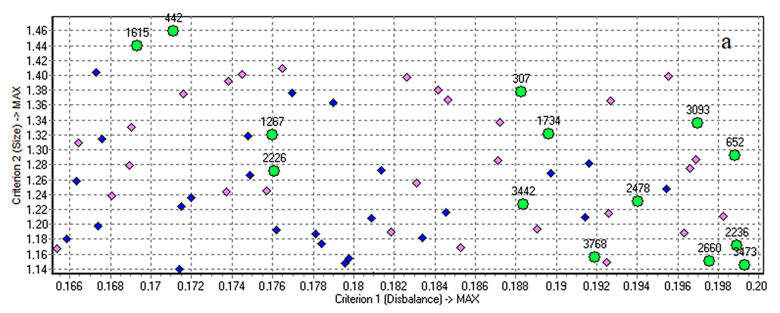
Let us consider in more detail how the criteria depend on the parameter $c_1$. The criterion $K_1$ depends on $c_1$ explicitly: the greater the load imbalance, the better. However, $K_1$ values greater than 0.2 are not required in practice. Therefore, in this problem, the values of $c_1$ vary from 0.3 to 0.7.

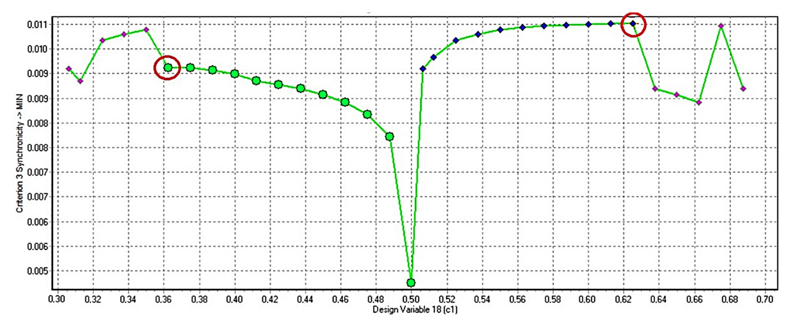
The criterion $K_2$ does not depend on $c_1$ at all. A typical example of the dependence of the criterion $K_3$ on $c_1$ is shown in Figure 2.

With an increase in the load imbalance, the synchronization of the actuators monotonically deteriorates, and asymmetrically when c1 deviates from 0.5 to the lower or higher side. However, starting from certain values of $c_1$, this dependence is violated, and the graph begins to behave unpredictably. In Figure 2 these points are circled in red. Solutions outside these $c_1$ values will be considered unacceptable. To detect such cases, for each checked value of $c_1$, we will perform several additional calculations with the load $c_1$ up to 0.5.

Additionally, it is necessary to take into account the asymmetry of the dependence of $K_3$ on $c_1$. For every feasible solution we obtain, the ultimate allowable load will be either less or greater than 0.5. For a symmetric case of unbalanced loads, the values of the criteria $K_1$ and $K_2$ will be the same, but the value of the criterion $K_3$ may be worse. However, we can switch this manipulator to a more advantageous (from the point of view of $K_3$) mode ($c_1>c_2$ or $c_1<c_2$), depending on how the load lies. Therefore, this asymmetry is not a problem.

5. Generation of Alternative Solutions and Initial Analysis

In the software MOVI, 4000 alternative solutions were generated, the coordinates of which are uniformly distributed in the space of variable parameters [20,21]. Of these solutions, 2198 were found to be feasible in relation to the constraints of the model. Among the feasible solutions, there were 96 Pareto optimal solutions. 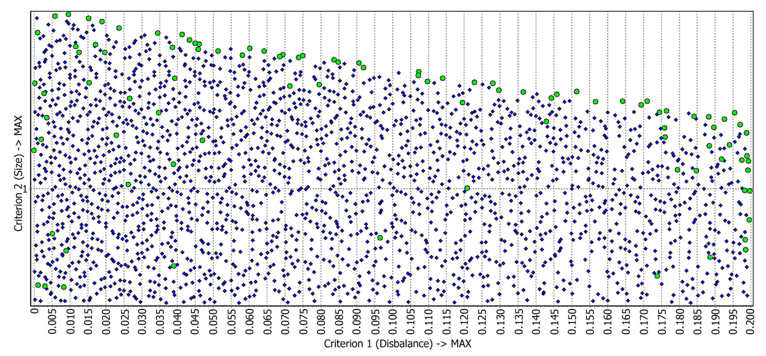Each solution x can be associated with a three-dimensional vector $K\left(x\right)=\left(K_1\left(x\right),K_2\left(x\right),K_3\left(x\right)\right)$, the components of which are estimates by three criteria. If the solutions are depicted as points in the three-dimensional space of criteria, then they form a cloud in a certain area, and the points of Pareto optimal solutions will be located on a part of the boundary of this cloud. In Figure 3 is shown how the projections of the cloud from the points of feasible solutions to the two-dimensional spaces of criteria are distributed. Blue rhombuses denote admissible solutions, green circles-Pareto optimal ones.

The depiction of the set of solutions in Figure 3 represent the initial, primary information for subsequent analysis and selection of the best solution. At the first stage, such images make it possible to assess in what ranges of criteria values are feasible solutions. That is, in fact, the decision maker (expert) receives primary information about the available opportunities in terms of achieving the best values of the criteria.

The first practical conclusion based on the analysis of Figure 3 is the following: a lot of feasible solutions are obtained with an acceptable value of the load imbalance $K_1$. Therefore, we can safely discard some of the solutions with weakly acceptable values of $K_1$, imposing an additional constraint on the feasibility of the solution $K_1>0.1$, and this leaves quite a lot of feasible solutions—821. Of these, 45 are Pareto optimal solutions. The values of the criteria for these 45 options are shown below in

Table 2. The values of the initial criteria and the obtained vector scores $y=(y_1,y_2,y_3)$ for 45 options.

No.	${\mathit{K}}_1$, ${10}^{-3}$	${\mathit{K}}_2$	${\mathit{K}}_3$, ${10}^{-3}$	${\mathit{y}}_1$	${\mathit{y}}_2$	${\mathit{y}}_3$	No.	${\mathit{K}}_1$, ${10}^{-3}$	${\mathit{K}}_2$	${\mathit{K}}_3$, ${10}^{-3}$	${\mathit{y}}_1$	${\mathit{y}}_2$	${\mathit{y}}_3$	No.	${\mathit{K}}_1$, ${10}^{-3}$	${\mathit{K}}_2$	${\mathit{K}}_3$, ${10}^{-3}$	${\mathit{y}}_1$	${\mathit{y}}_2$	${\mathit{y}}_3$
159	1.30	1.52	12.4	3	10	3	1267	1.76	1.32	3.7	8	8	10	2660	1.98	1.15	4.6	10	6	9
239	1.14	1.58	11.1	2	10	4	1382	1.64	1.46	7.4	7	9	7	2834	1.51	1.51	5.1	6	9	9
247	1.98	0.73	4.5	10	2	9	1615	1.69	1.44	5.2	7	9	9	2841	1.76	1.41	16.2	8	9	1
257	1.43	1.35	3.0	5	8	10	1691	1.37	1.51	4.9	4	9	9	3005	1.28	1.55	7.7	3	10	7
307	1.88	1.38	6.5	9	8	8	1734	1.90	1.32	6.3	9	8	8	3093	1.97	1.34	7.5	10	8	7
442	1.71	1.46	6.8	8	9	7	1760	1.46	1.50	5.0	5	9	9	3254	1.99	0.68	4.7	10	2	9
464	1.99	1.10	5.8	10	6	8	1847	1.96	1.40	13.8	10	8	2	3298	1.98	0.99	4.4	10	5	9
635	2.00	0.84	7.8	10	3	7	1849	1.79	1.10	3.5	8	6	10	3423	1.20	1.45	3.2	2	9	10
652	1.99	1.29	6.4	10	7	8	2010	1.84	1.38	10.0	9	8	5	3442	1.88	1.23	3.5	9	7	10
840	1.89	0.64	3.1	9	1	10	2057	1.10	1.56	8.6	1	10	6	3473	1.99	1.14	8.2	10	6	6
895	1.07	1.61	8.7	1	10	6	2112	1.75	1.40	12.2	8	8	4	3642	2.00	0.99	8.1	10	5	7
911	1.57	1.46	4.5	6	9	9	2226	1.76	1.27	6.3	8	7	8	3768	1.92	1.16	3.6	10	6	10
997	1.85	1.10	3.2	9	6	10	2236	1.99	1.17	6.5	10	6	8	3862	1.74	0.54	2.7	8	1	10
1080	1.44	1.48	3.5	5	9	10	2276	1.23	1.56	10.3	3	10	5	3900	1.93	1.37	11.8	10	8	4
1246	1.07	1.59	4.0	1	10	10	2478	1.94	1.23	3.7	10	7	10	3952	1.21	1.00	3.0	3	5	10

. The result of imposing this restriction in the criteria space is shown in Figure 4.

We see that in the projections onto $K_1$ and $K_2$ (Figure 4a,b), the set of solutions is expectedly divided into feasible (to the right of the line $K_1=0.1$) and infeasible (to the left of the line $K_1=0.1$). Its analysis helps to verify, to make sure that the imposed constraint on the criterion $K_1$ led to acceptable impairments in the remaining criteria.

Further, you can also impose constraints on the remaining criteria, and then gradually increase these constraints, thereby narrowing the set of choices. This is one of the approaches, it can be classified as intuitive, informal. Its application becomes much more complicated with a larger number of criteria. To solve the problem of choosing the best solution in this work, we will apply the formal approach developed in the criteria importance theory.

6. Solving the Choice Problem by the Method of the Criteria Importance Theory

It is required to choose the best solution among the selected 45 solutions obtained at the previous stage, taking into account the constraint $K_1>0.1$.

To apply the methods of the criteria importance theory, the individual criteria $K_1$, $K_2$, $K_3$ must be brought to a homogeneous form with a common scale Z, which can be just ordinal [26]. In this problem, we will use a 10-point scale: the higher the score, the better, the higher the value (usefulness, preference) for the decision maker of such values according to the criterion. To bring the criteria to the 10-point scale Z, we use linear normalization of the criteria values and rounding. As a result, each of the 45 alternative solutions is associated with its vector score from the set $Z^3=Z\times Z\times Z$. The values of the initial criteria and the obtained vector scores $y=(y_1,y_2,y_3)$ for all 45 options are given in Table 2. It should be noted that the requirements for minimization and maximization for the initial criteria can be different ($K_1\to max$, $K_2\to max$, $K_3\to min$), while the scores on the scale Z are always the same ($y_1\to max$, $y_2\to max$, $y_3\to max$).

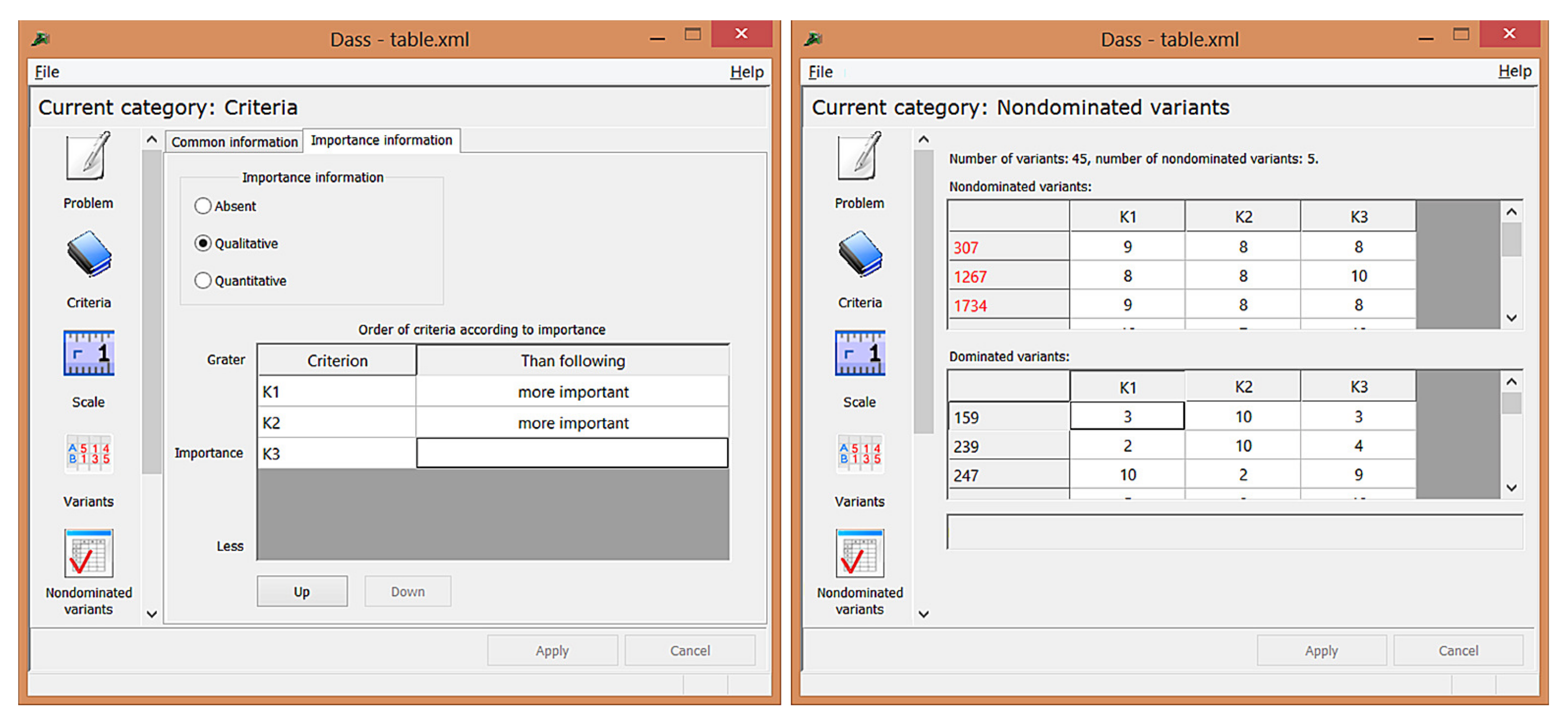
In fact, due to rounding, each vector score describes a certain small region in the original 3D space of the criteria. At the same time, some solutions may be in the same region, and then they will have the same vector score. For example, alternatives 307 and 1734 have the same vector score (9, 8, 8). Further, using the method of the criteria importance theory, we will solve the problem of choosing the best vector score. Choosing this vector score, we will obtain a corresponding small region in the original space of criteria, which includes one or more solutions from the 45 considered.

In the criteria importance theory, the preferences of decision makers are modeled using binary relations [26]. The non-strict preference relation R of the decision maker is introduced on the set of vector scores $Z^3$: the notation $yRz$ means that the vector score y is no less preferable than z. The relation R is reflexive and transitive, it generates the relations of indifference (equivalence) I and strict preference (dominance) P:

$$\begin{array}{c}yIz\iff yRz\mathrm{and}zRy,\\ yPz\iff yRz,\mathrm{but}zRy\mathrm{is}\mathrm{not}\mathrm{true}.\end{array}$$

It is known that if the relation R is complete, then on a finite set of vector scores there is at least one optimal vector score y, such that $yRz$ holds for all other vector scores z. There can be several optimal vector scores equivalent by the relation I. In this case, the choice of the best vector score should be carried out among the optimal vector scores.

If the relation R is incomplete, then the best vector score should be chosen among the non-dominated vector scores. A vector score y is called non-dominated with respect to P if there is no other vector score z, such that $zPy$ holds.

Since the decision maker’s preferences increase along the scale of criteria Z, the Pareto relation is defined on the set of vector scores $Z^3$:

$$\begin{array}{c}y{R}^{\oslash }z\iff y_i\ge z_i,i=1,2,3;\\ y{P}^{\oslash }z\iff y{R}^{\oslash }z\mathrm{and}y\ne z.\end{array}$$

Among the 45 vector scores under consideration, there are 10 non-dominated with respect to the Pareto relation $P^{\oslash }$. In fact, 9 vector scores remain, since variants with numbers 307 and 1734 have the same vector score (9, 8, 8). These vector scores and the corresponding alternatives are shown in

Table 3. 10 vector scores and their the corresponding alternatives.

No.	${\mathit{K}}_1$	${\mathit{K}}_2$	${\mathit{K}}_3$	${\mathit{y}}_1$	${\mathit{y}}_2$	${\mathit{y}}_3$
307	0.188	1.38	0.0065	9	8	8
442	0.171	1.46	0.0068	8	9	7
1080	0.144	1.48	0.0035	5	9	10
1246	0.107	1.59	0.0040	1	10	10
1267	0.176	1.32	0.0037	8	8	10
1615	0.169	1.44	0.0052	7	9	9
1734	0.190	1.32	0.0063	9	8	8
2478	0.194	1.23	0.0037	10	7	10
3005	0.128	1.55	0.0077	3	10	7
3093	0.197	1.34	0.0075	10	8	7

.

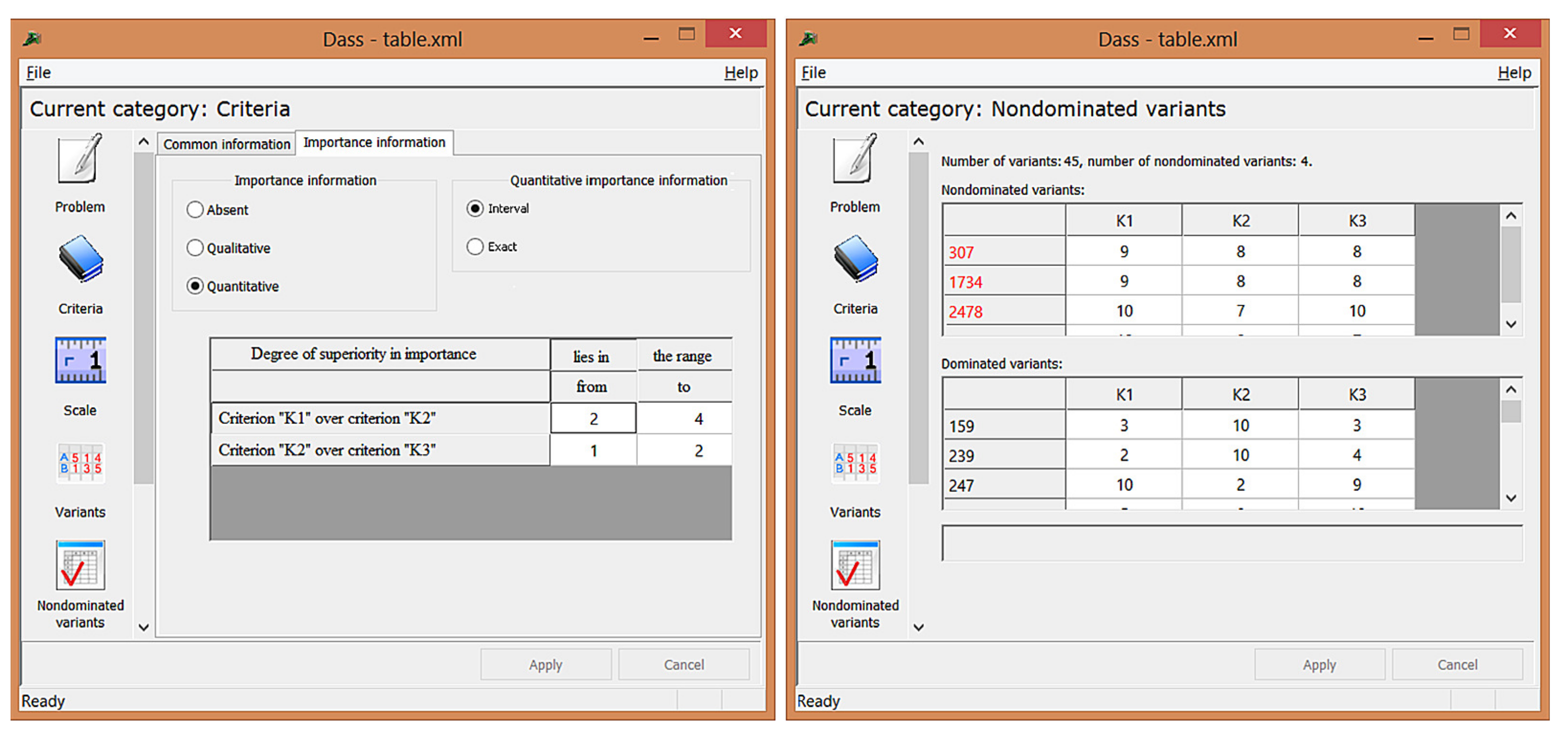
At the next step of solving the choice problem by the criteria importance method, we enter information $\mathsf{\Omega }$ about the ordering of criteria by importance into the software DASS, as shown in Figure 5 [27,29]. The criterion $K_1$ is more important than the criterion $K_2(1\succ 2)$, and the criterion $K_2$, in turn, is more important than the criterion $K_3(2\succ 3)$.

As a result, there are only 4 non-dominated vector scores and the corresponding 5 alternative solutions shown in

Table 4. The 4 non-dominated vector scores and the corresponding 5 alternative solutions.

No.	${\mathit{y}}_1$	${\mathit{y}}_2$	${\mathit{y}}_3$	Value Function Estimation
307; 1734	9	8	8	0.846
1267	8	8	10	0.802
2478	10	7	10	0.907
3093	10	8	7	0.901

. For each of the 5 vector scores that turned out to be dominated with respect to $P^{\mathsf{\Omega }}$, it is possible to formally explain why it should be excluded from consideration. Namely, what other vector score dominates it and on the basis of what information about preferences this conclusion is made:

$$\begin{array}{c}y\left(307\right)=(9,8,8)P^{1\succ 2}(8,9,8)P^{\oslash }(8,9,7)=y\left(442\right),\\ y\left(2478\right)=(10,7,10)P^{1\succ 2}(7,10,10)P^{\oslash }(5,9,10)=y\left(1080\right),\\ y\left(2478\right)=(10,7,10)P^{1\succ 2}(7,10,10)P^{\oslash }(1,10,10)=y\left(1246\right),\\ y\left(2478\right)=(10,7,10)P^{1\succ 2}(7,10,10)P^{\oslash }(7,9,9)=y\left(1615\right),\\ y\left(2478\right)=(10,7,10)P^{1\succ 2}(7,10,10)P^{\oslash }(3,10,7)=y\left(3005\right),\\ \end{array}$$

For example, the notation (10, 7, 10)$P^{1\succ 2}$ (7, 10, 10) means that the vector score (10, 7, 10) is preferable to the vector score (7, 10, 10), since the first criterion is more important than the second. As we can see from the constructed chains of vector scores, in this case, in order to discard the vector scores dominated by $P^{\mathsf{\Omega }}$ from the information $\mathsf{\Omega }$ about the ordering of criteria by importance, it turned out to be enough to use only the fact that the first criterion is more important than the second.

The resulting 4 vector scores remain incomparable with the introduced information about the DM’s preferences. Next, we will analyze them from different angles. At this stage, the value functions of these vector scores can be estimated by calculating the centroid values of the decision maker’s preference parameters [28]. Figure 6 shows how to do this in the software DASS, Table 4 shows the resulting values of the value functions.

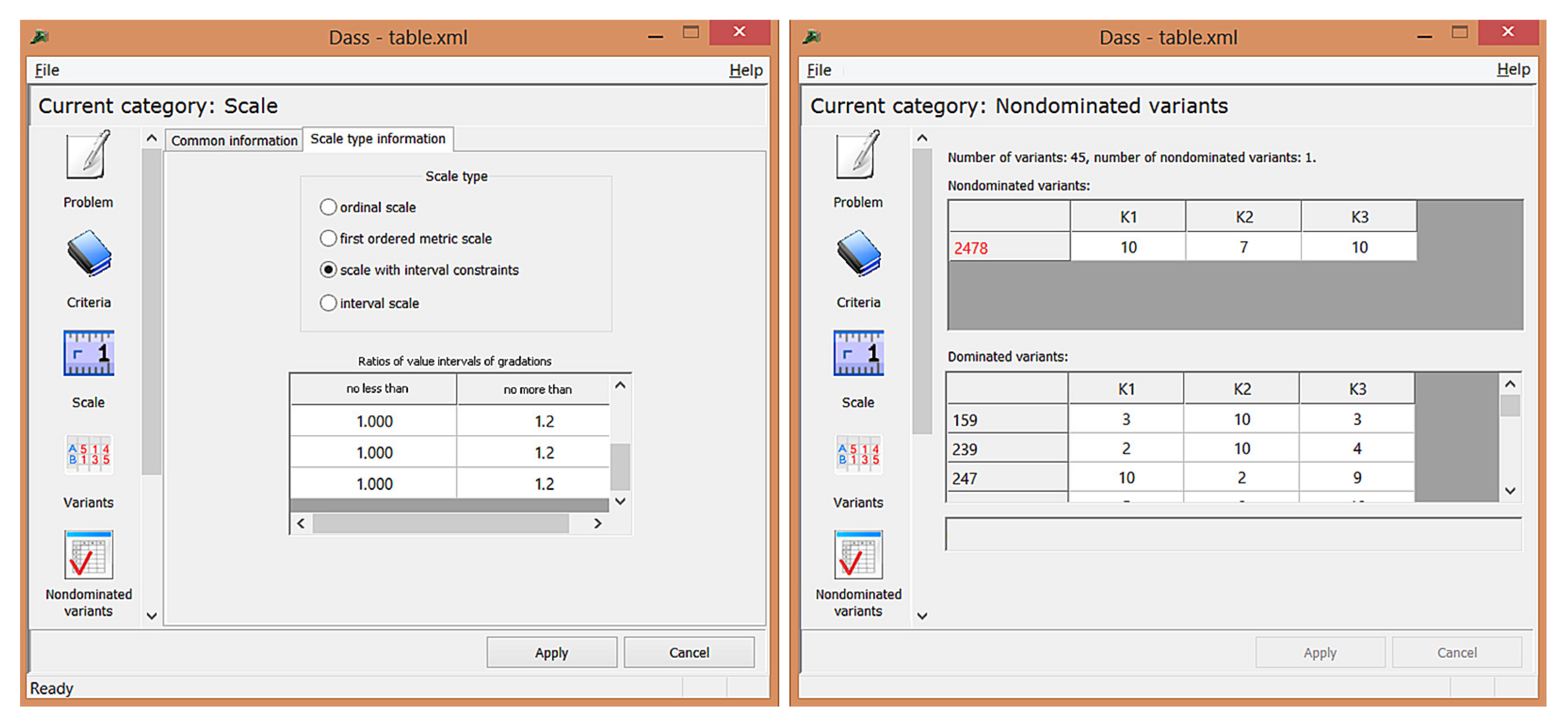
Let us continue the formal solution of the choice problem by the criteria importance method. At the next step, we input in the software DASS (see Figure 7) interval information about the relative importance of the criteria: the first criterion is at least 2 times more important than the second, and no more than 4 times; the second criterion is no more than 2 times more important than the third.

With such information about the preferences of the decision maker, the vector score $y\left(1267\right)=(8,8,10)$ turns out to be dominated.

Table 5. The remaining non-dominated vector scores.

No.	${\mathit{y}}_1$	${\mathit{y}}_2$	${\mathit{y}}_3$	Value Function Estimation
307; 1734	9	8	8	0.978
2478	10	7	10	0.983
3093	10	8	7	0.980

shows the remaining non-dominated vector scores. Their value functions have changed slightly, as the set of possible values of preference parameters has changed (narrowed) and the corresponding centroid values of these parameters have shifted.

At the next step in solving the choice problem, let us clarify the information on how the decision maker’s preferences grow along the criterion scale Z (see Figure 8).

As a result, there is only one non-dominated vector score (10, 7, 10), which corresponds to the solution 2478. Additionally, in favor of this vector score, we can note the fact that the estimation of its value function was higher than others at each step of solving the problem.

The only solution was selected using imprecise information about the preferences of experts, given in the form of interval estimates. In the previous steps, the choice set was significantly narrowed down based only on qualitative assessments of preferences. The use of partial and imprecise information about the preferences, an iterative procedure for clarifying this information, as well as the ability to formally substantiate the conclusions made are significant advantages of the considered method of the criteria importance theory in comparison with other methods of multicriteria analysis.

7. Additional Visual Analysis of Alternative Solutions

After the formal analysis of the problem by the criteria importance methods, it is useful to return to the graphical representations of the solutions. Consider 4 non-dominated vector estimates and the corresponding 5 solutions listed in Table 4. Recall that they are selected after a simple ordering of the criteria by importance.

Let us see where these solutions are in the space of the initial criteria $K_1$, $K_2$, $K_3$. To do this, we introduce additional constraints on the values of criteria in the software MOVI. Note that the considered vector scores have the minimum values of the components $y_1$, $y_2$, $y_3$ equal to 8, 7, 7, respectively. In order for only solutions with estimates $y_1\ge 8$, $y_2\ge 7$, and $y_3\ge 7$ to remain feasible, the following constraints should be imposed on the values of the criteria: $K_1>0.17$, $K_2>1.188$, and $K_3<0.0081$. The result is shown in Figure 9.

Figure 9 gives a general idea in which region of the original point cloud of all solutions the solutions we have selected turned out to be. Now, let us zoom in on the display area. In addition, we will slightly weaken the constraints on the criteria in order to exclude the rounding effect in the process of bringing the criteria to the 10-point scale: $K_1>0.165$, $K_2>1.134$ and $K_3<0.0088$. This extended sample contains 39 solutions, including 14 Pareto optimal solutions. The result is shown in Figure 10.

In Figure 10, the numbers of other solutions, in addition to the selected 5 solutions from Table 4, are marked. In these scaled figures, it is possible to compare different solutions in pairs. In particular, to make sure that the solution 2478, chosen by the formal method, is preferable. It is also interesting to compare the solutions 307 and 1734, which are located side by side on all three projections and have the same vector score.

8. Result and Discussion

After carrying out a numerical experiment, out of the generated 4000 solutions, only 2198 were found to be feasible in relation to the constraints of the model. Among such an abundance of solutions, it is impossible to choose the best one by examining the three-dimensional space of optimization criteria. Obtaining the set of Pareto optimal solutions allowed us to select 96 solutions. Further, the analysis of the criteria space was carried out in order to reduce the area of suitable solutions, and preferences were introduced regarding the importance and values of the criteria. Thus, we reduced the number of best solutions to 10 (Table 3), and subsequently chose one best solution. Further, the analysis of the obtained solutions is advisable to carry out using a visual analysis of solutions as shown in [11]. Here is a description of the selected solutions.

Table 6. The optimized parameters of the system and the ranges of their values.

Parameter	Range	307	1267	1734	2478	3093
$c_1$	$0.3÷0.7$	0.688	0.676	0.690	0.694	0.697
${\chi }_L$	$-2.0÷-0.4$	−1.378	−1.320	−1.321	−1.230	−1.336
${\lambda }_V$	$0.2÷1.0$	0.839	0.847	0.511	0.567	0.726
${\beta }_0$	$0.3÷0.7$	0.507	0.678	0.433	0.630	0.688
${\alpha }_1$	$0.25÷1.0$	0.779	0.964	0.800	0.801	0.676
${\alpha }_2$	$0.25÷1.0$	0.295	0.625	0.598	0.746	0.435
${\kappa }_1$	$0.05÷0.1$	0.059	0.057	0.052	0.087	0.052
${\kappa }_2$	$0.05÷0.1$	0.063	0.095	0.060	0.055	0.074
${\vartheta }_1$	$25÷50$	46.729	44.714	37.561	38.153	43.732
${\vartheta }_2$	$0÷50$	30.566	17.407	1.831	33.533	13.293
${\vartheta }_D$	$25÷50$	72.314	83.777	87.366	95.880	38.715
${\vartheta }_V$	$0÷5$	4.990	0.881	2.986	2.882	3.578
$t_A$	$0.02÷0.04$	0.034	0.024	0.020	0.027	0.027
$t_B$	$0.02÷0.04$	0.031	0.023	0.028	0.040	0.035
${\chi }_{L1}$	$0÷0.1$	0.001	0.056	0.005	0.048	0.096
${\chi }_{L2}$	$0÷0.1$	0.036	0.038	0.078	0.088	0.039
${\lambda }_{01}$	$0.05÷1.0$	0.05	0.05	0.05	0.05	0.05
${\lambda }_{02}$	$0.05÷1.0$	0.05	0.05	0.05	0.05	0.05
${\tau }_S$	$10÷50$	44.453	28.574	26.738	20.576	30.596

shows the values of the optimized parameters for the selected solutions, as well as in Figure 11 and Figure 12 are a visual representation of the dynamic characteristics. A more detailed description of the visualization principles is presented in [11].

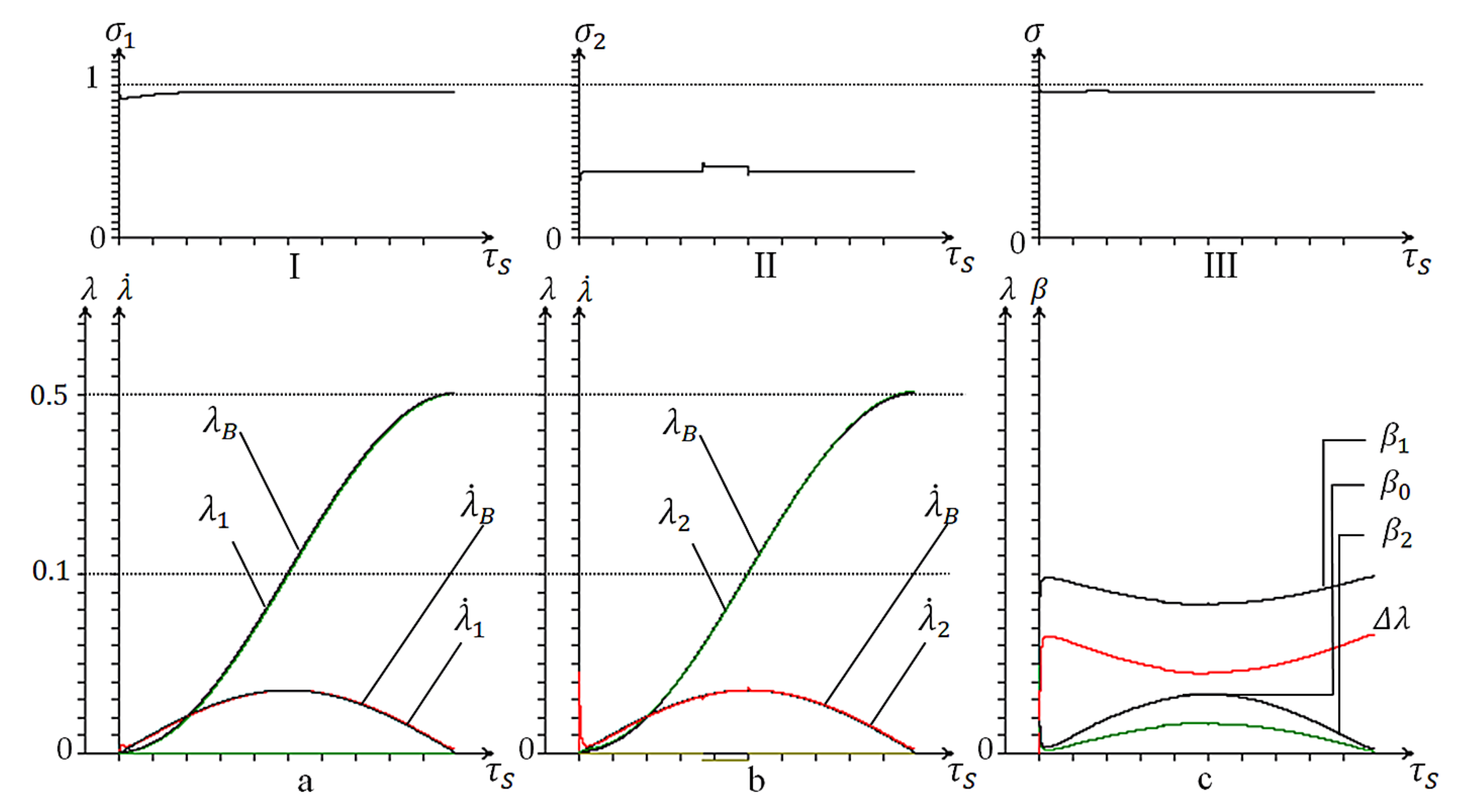
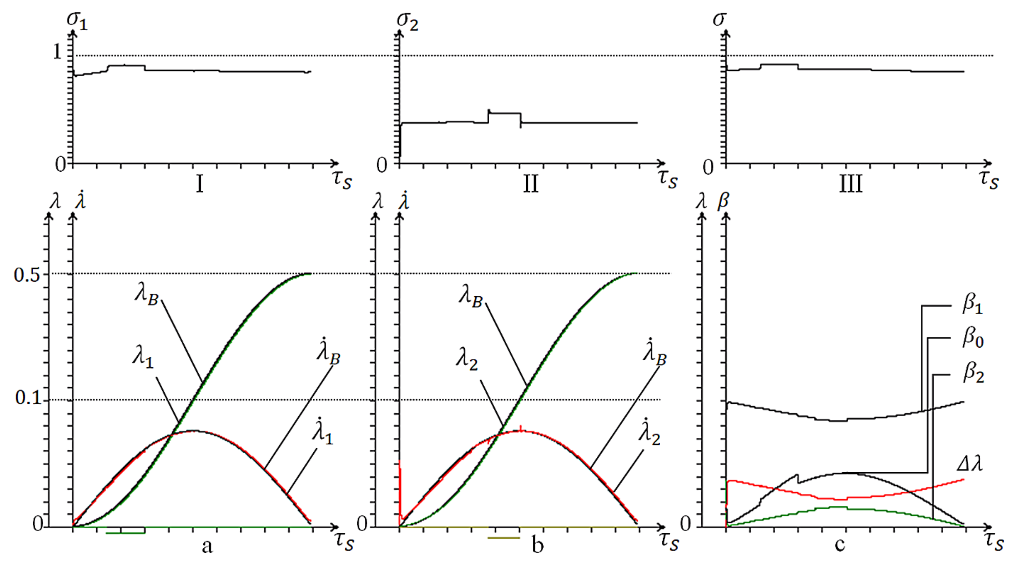
Figure 11 shows the characteristics of the movement of the system of the solution 307 with unequal mass loads on the first and second actuators ($c_1=0.688$, $c_2=0.312$):

(a)

indicators of the first actuator: curves of displacement and speed (${\lambda }_1$, ${\dot{\lambda }}_1$); in the upper part of this column I—pressure in its working cavity (${\sigma }_1$);

(b)

indicators of the second actuator: curves of displacement and speed (${\lambda }_2$, ${\dot{\lambda }}_2$); in the upper part of this column II—pressure in its working cavity (${\sigma }_2$);

(c)

channel opening curves (${\beta }_0$, ${\beta }_1$, ${\beta }_2$): changes in the mismatch criterion $\Delta \lambda$ in the movement of actuators, III—pressure in the intermediate cavity ($\sigma$).

The designations for these quantities were explained in the previous section. The curves in Figure 12 are arranged in the same order.

The values of all parameters for each solution can be viewed in Table 6. The scale for displacement $\lambda$ is doubled relative to the pressure $\sigma$. The scale in speed $\dot{\lambda }$ is ten times the pressure. The $\beta$ scale (flow area value) is increased five times relative to the pressure.

It follows from the graphs that under the conditions of the optimized solution 307 (Figure 11), despite the high load level of the actuators ($|{\chi }_L|=1.378$), and the imbalance in loading the right and left cargo ($c_1=0.688$, $c_2=0.312$), the given laws of motion actuators are implemented with good accuracy, and the pressures in all cavities after a short-term initial disturbance quickly stabilize and are practically invisible.

A short-term disturbance in the system is modeled by a variable ${\chi }_{L1,2}$, in Table 6 these are the variables ${\chi }_{L1}$ and ${\chi }_{L2}$. The first actuator is supplied with an additional load ${\chi }_{L1}=0.001$, and practically does not affect the positioning process, the second actuator is supplied with ${\chi }_{L2}=0.036$, and we see a small jump in pressure ${\sigma }_2$, which also insignificantly affects the positioning process. The operation of the system under the conditions of the solution 307 is distinguished by a very low sensitivity to variations in position and speed (${\lambda }_1$, ${\dot{\lambda }}_1$) parameters within the entire selected range.

The solution 2478 shows in Figure 12, in which unequal mass loads on the first and second actuators ($c_1=0.694$, $c_2=0.306$), short-term disturbances in the system (${\chi }_{L1}=0.048$ and ${\chi }_{L2}=0.088$) are set. Despite the more significant short-term disturbances, we see pressure surges in both actuators (${\sigma }_1$ and ${\sigma }_2$ graph), which practically does not affect the positioning process. This is primarily due to the correct choice of the remaining parameters of the optimized system. In [11], variants are presented when, for other parameters, but weaker perturbations, the system does not behave stably.

From a computational point of view, the process of generating 4000 alternative solutions in the MOVI software took the longest time—about 3 h on a personal computer. Each of these solutions had to be checked for feasibility, and, for this, the system of Equation (6) had to be solved by the Runge–Kutta method several times for different values of the parameter c1. On average, it took 15 such launches and 2.7 s to check one solution. All other calculations took almost no time and were invisible for experts working with the systems. The operation of decision rules in the DASS system in problems with up to 10 criteria takes less than a second [27]. Such problems of designing new mechanisms are one-off, individual, so it is permissible and even advisable to spend a lot of time on solutions search and careful analysis.

9. Conclusions

The procedure used in this work is based on two important factors: a rational mathematical model and a rational optimizing method. The effectiveness of the proposed procedure is shown by the example of solving a complex dynamic problem-choosing the best option for a technical project. The first factor made possible to simplify to the limit a real computational model by reducing the number of both parameters and criteria, which are considered as a purely physical value. The second factor allowed us to enter the area of best solutions with a significant reduction in options variation. In conclusion, we note the following main stages of work:

–

Developing a mathematical model of the investigated physical object;

–

Transition to dimensionless parameters;

–

On the basis of a dimensionless mathematical model of a physical object, multi-parameter and multicriteria optimization is carried out with the selection of the Pareto set;

–

Analysis of the criteria space in order to reduce the area of suitable solutions;

–

Preferences are introduced regarding the importance and values of criteria in the form of qualitative or imprecise quantitative (interval) estimates;

–

Visual analysis of the received solutions.

As an additional stage, the proposed procedure can also include an optimization stage in the transition from dimensionless to dimensional values. The technical design of a robotic system with two actuators operating in accordance mode, considered as an example, shows the effectiveness of the approach proposed.