
A Global Optimization Algorithm for Solving Linearly Constrained Quadratic Fractional Problems

College of Science, Zhejiang University of Technology, Hangzhou 310023, China
*
Author to whom correspondence should be addressed.
Mathematics 2021, 9(22), 2981; https://0-doi-org.brum.beds.ac.uk/10.3390/math9222981
Submission received: 18 September 2021
/
Revised: 8 November 2021
/
Accepted: 17 November 2021
/
Published: 22 November 2021
Abstract
:This paper first proposes a new and enhanced second order cone programming relaxation using the simultaneous matrix diagonalization technique for the linearly constrained quadratic fractional programming problem. The problem has wide applications in statics, economics and signal processing. Thus, fast and effective algorithm is required. The enhanced second order cone programming relaxation improves the relaxation effect and computational efficiency compared to the classical second order cone programming relaxation. Moreover, although the bound quality of the enhanced second order cone programming relaxation is worse than that of the copositive relaxation, the computational efficiency is significantly enhanced. Then we present a global algorithm based on the branch and bound framework. Extensive numerical experiments show that the enhanced second order cone programming relaxation-based branch and bound algorithm globally solves the problem in less computing time than the copositive relaxation approach.
1. Introduction
The quadratic fractional programming problem refers to with and being quadratic functions and the feasible region . It has many applications in electric engineering [1], finance, production planning [2], and communications over wireless channels [3] etc. Many strategies have been developed to solve this important issue. One classical approach is the Dinkelbach method proposed by Dinkelbach [4]. For example, Salahi et al. [5] studied the problem of minimizing the ratio of two indefinite quadratic functions subject to a strictly convex quadratic constraint. Zhang et al. [6] proposed a Celis-Dennis-Tapia based approach to quadratic fractional programming problems with two quadratic constraints. Gotoh et al. [3,7] solved the general quadratic fractional problems by combing Dinkelbach iterative algorithm with the branch and bound algorithm together. Moreover, the metaheuristics-based approaches successfully combining machine learning and swarm intelligence were able to solve the problem globally [8,9]. In recent years, the semidefinite programming (SDP) relaxation and the copositive relaxation have become popular to solve the quadratic fractional programming problems. Some special case of the quadratic fractional programming problem can be reformulated into an exact SDP relaxation and solved in polynomial time. Beck et al. [10] showed that minimizing the ratio of indefinite quadratic functions over an ellipsoid admitted an exact SDP reformulation under some technical conditions. Xia [11] improved their results by removing the technical conditions. Nguyen et al. [12] analysed quadratic fractional problems over a two-sided quadratic constraint with three cases and illustrated that each of them admited an exact SDP relaxation. Moreover, Preisig [13] used the idea of copositivity to deal with the standard quadratic fractional functions. Amaral et al. [14] proposed a copositive relaxation for nonconvex min-max fractional quadratic problems under quadratic constraints and showed that the lower bound provided by the copositive relaxation could speed up a well-known solver in obtaining the optimal value.
In this paper, we consider the quadratic fractional programming with linear constraints:
The above problem was proposed by Amaral et al. [15]. Interesting applications of (1) include the standard quadratic fractional problem and the symmetric eigenvalue complementarity problem. Here, is a symmetric matrix, , , and . Without loss of generality, we assume that A is full row rank. When Q is semidefinite, it becomes the total least squares, and is thus widely used in a variety of disciplines such as statics, economics and signal processing [16]. In this paper, is supposed to be nonempty and compact, i.e., and . The nonconvexity of the objective function leads to the challenge in solving this problem. Amaral et al. [15] proposed a copositive (CP) relaxation for the problem. Although they showed that the CP relaxation admitted a better lower bound including small relative gaps with the optimal value, the computational complexity was high as shown in their numerical results [15]. In particular, the CPU spent more than 50 s to solve the CP relaxation when the dimension of variables was 79. Thus, designing a convex relaxation that can be efficiently used even for huge-size problem while maintaining the strength of the convex relaxation is critical. In this paper, we design an enhanced second order cone programming (SOCP) relaxation for (1) instead. We first reformulate the primal problem into a quadratic programming problem with a quadratic equality and linear constraints. Furthermore, we present an enhanced SOCP relaxation exploiting the simultaneous matrix diagonalization tool. We compare the enhanced SOCP relaxation with the classical SOCP relaxation, and extensive numerical experiments verify that the enhanced SOCP relaxation shows superiority in both the relaxation effect and computational complexity. In particular, the superiority is magnified when the number of the negative eigenvectors of Q increases. Then we design a branch and bound algorithm based on the enhanced SOCP relaxation to find the optimal solution. Numerical experiments show that though the lower bound provided by the enhanced SOCP relaxation is worse than that of the CP relaxation, the computational complexity is much lower. Thus, the enhanced SOCP relaxation-based branch and bound algorithm spends much less time to obtain the optimal solution than that of the CP relaxation when the dimension of the variables is more than 100.
The following notations are adopted throughout the paper. Given a real symmetric matrix X, means X is positive semidefinite. I denotes an identity matrix. For n by n real matrices and , trace. represents that is rounded down to the nearest integer. Given a vector , corresponds to an diagonal matrix with its diagonal elements equal to b.
The paper is organized as follows. In Section 2, we recast the problem into a quadratic programming problem with a quadratic equality and linear constraints and then present an enhanced SOCP relaxation. Section 3 describes a branch and bound algorithm. Section 4 provides numerical experiments to verify that the enhanced SOCP relaxation-based branch-and-bound method is effective to solve the problem. Conclusions are given in Section 5.
2. A Reformulation of (1) and an Enhanced SOCP Relaxation
Some constrained quadratic fractional problems are equivalent to quadratically constrained quadratic programming problems [13,15]. Following this idea, in this section we first equivalently reformulate (1) into a quadratically constrained quadratic programming problem and then design an enhanced SOCP relaxation.
For convenience, let , , , then (1) equals to the following homogeneous quadratic fractional program with linear constraints:
If we define , then (2) is recast into:
Lemma 1.
(2) is equivalent to (3).
Proof.
If z is a feasible solution of (2), then let . It is easy to verify that y is a feasible solution of (3) and . Hence, the optimal value of (3) is no more than that of (2). Conversely, if y is a feasible solution of (3), then implies that . Let with and . If , then and . Hence, , which contradicts with the conclusion that . Therefore, . Let , then it is easy to verify that z is a feasible solution of (2) and . Hence, the optimal value of (3) is no less than that of (2). Consequently, (2) is equivalent to (3). □
Lemma 1 leads directly to the following proposition.
Proposition 1.
(1) is equivalent to (3).
Therefore, in order to solve (1), we would like to solve (3) instead. Since there is an equality constraint in (3), we first reduce the variable dimension from to by employing a similar method as in [15]. Let be an orthonormal basis of ker , thus, y can be written as with on condition that y satisfying . Let and , then (3) turns into:
(4) is a nonconvex quadratic program with one spherical constraint and linear constraints. In general, it cannot be solved in polynomial time. Amaral et al. [15] proposed a CP relaxation for (1):
They showed that the CP relaxation could provide a good lower bound and numerical experiments also verified that the CP relaxation resulted in small relative gaps with the optimal value. However, the computational complexity is high. Thus, it is not effective to solve the problem when the dimension of variables becomes larger. In contrast, the classical SOCP relaxation has much lower computational complexity, but its relaxation effect is worse [17]. To balance the relaxation effect and computational complexity, we design an enhanced SOCP relaxation which could both improve the lower bound and reduce the computation time compared to the classical SOCP relaxation.
Next, we first briefly introduce the classical SOCP relaxation. We decompose by eigenvalue decomposition, where are eigenvalues and are corresponding eigenvectors, for . Let s denote the number of negative eigenvalues of . The lower bound and upper bound of are solved by and for , respectively. Moreover, the lower bound and upper bound of are solved by and for , respectively. Then the classical SOCP relaxation becomes [17]:
In what follows, we design a new SOCP relaxation by employing the simultaneous matrix diagonalization technique. The simultaneous matrix diagonalization-based convex relaxation was first proposed to solve the one quadratically constrained quadratic program on condition that the quadratic forms are simultaneously diagonalizable by Ben-Tal et al. [18]. Then Zhou et al. used the simultaneous matrix diagonalization technique to solve various problems including the convex quadratic program with linear complementarity constraints [19], the generalized trust-region problem [20], and the convex quadratically constrained nonconvex quadratic programming problem [21]. All of the above research implies that convex relaxations employing the simultaneous matrix diagonalization to solve some special quadratically constrained quadratic programming problems could result in a better lower bound or reduce the computational complexity.
It is obvious that I and can be simultaneously diagonalizable, i.e., there exists a nonsingular matrix V such that and are both diagonal matrices. In fact, let by using eigenvalue decomposition where and , then and . Let , then (4) becomes:
The lower bound and upper bound of are solved by and for , respectively. We derive a new SOCP relaxation by relaxing into for :
We observe that (6) has s more convex quadratic constraints and s more linear constraints than those of (8); hence, the computational complexity of (6) is higher. Moreover, the auxiliary variables and are only bounded above by linear constraints in (6), in contrast, the auxiliary variable is not only bounded above by the linear constraints, but also appears in the objective function. Thus, minimizing the objective function also prevents the auxiliary variables from going to infinity when .
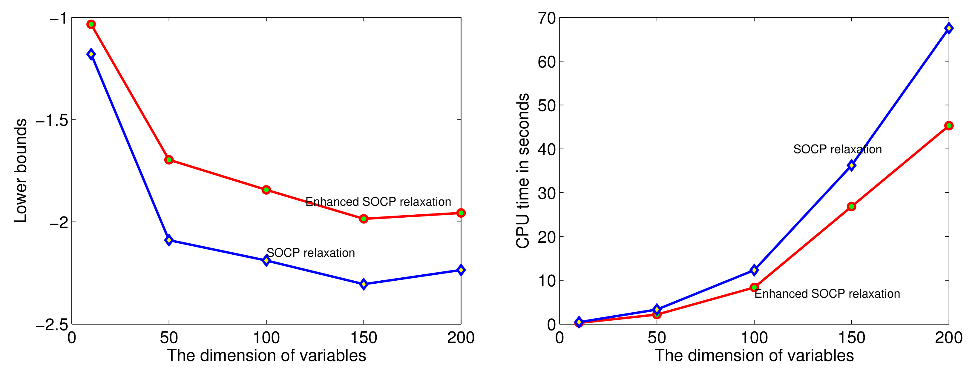
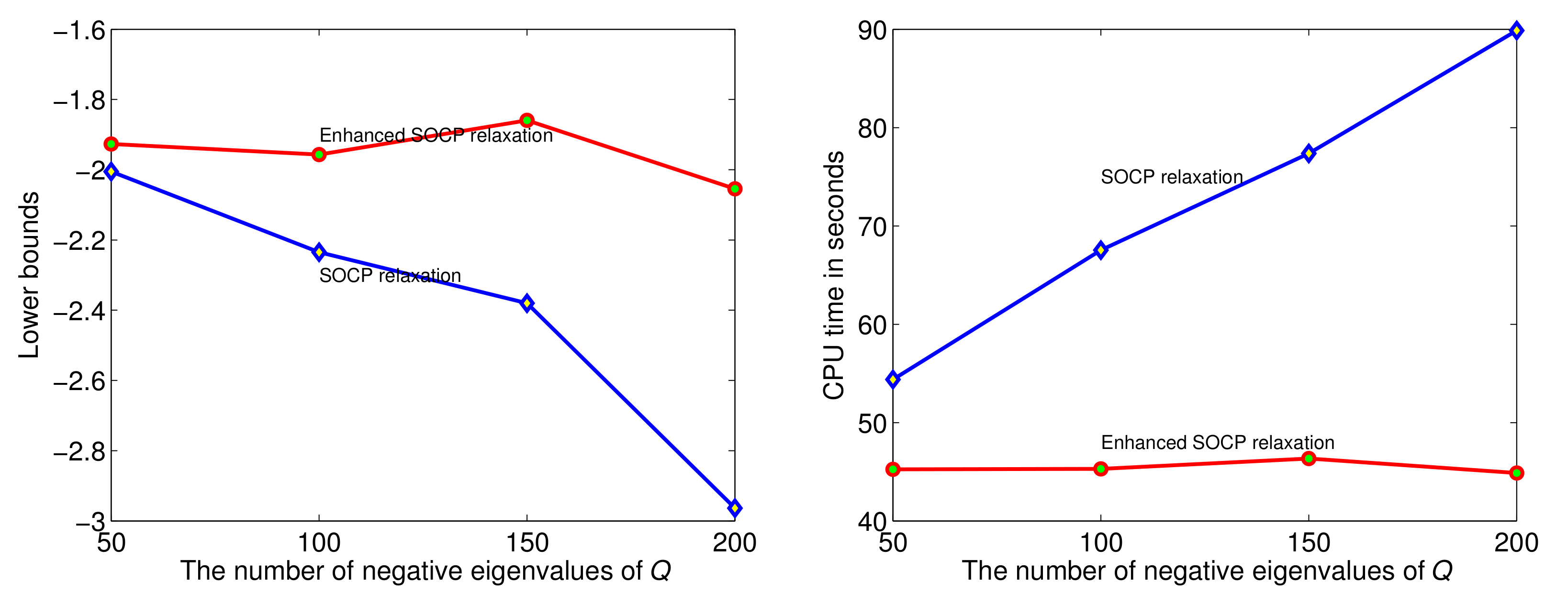
To verify that (8) indeed enhance the relaxation effect of the classical SOCP relaxation (6), we use some randomly generated instances to test the two relaxations. Five instances are generated for each given problem size. The average lower bounds and average computing time in seconds are computed. The concrete generation process of random examples are described in Section 4. In Figure 1, we let , and , where r denotes the number of negative eigenvalues of the objective function matrix Q. To compare the two relaxations varying from r, we set , and and the results are listed in Figure 2.
Figure 1 shows that (8) obtains a better lower bound in less computing time than that of (6). Moreover, the advantage of computing time is highlighted when the dimension increases.
Figure 2 shows that the relaxation effect and computing time of (8) change very little with the varying number of negative eigenvalues of Q. In contrast, the relaxation effect of (6) becomes worse and the computing time increases when the number of negative eigenvalues of Q becomes larger. Hence, we conclude that the advantages of both the relaxation effect and computing time of (8) are highlighted as the number of negative eigenvalues of Q increases.
3. An Enhanced SOCP Relaxation Based Branch-and-Bound Algorithm
The branch and bound algorithm is widely used for globally solving constrained fractional programming problems [22], thus, we present an enhanced SOCP relaxation-based branch-and-bound scheme detailed in Algorithm 1 for (7) in this section. There are four steps in the design framework:
(1) Initialization. Set the initial lower bound and for . Solve (8) with to obtain its optimal value and optimal solution .
(2) The node selection strategy. The algorithm employs the classical “best-first” selection strategy, i.e., the one with the lowest bound among the live subproblems is selected.
(3) The variable selection strategy and branching rule. Let be the solution of (8) at the current node k over the box . Choose . Then the box is split into two sub-boxes and with , for and , , for and . Thus, two new subproblems are generated over the two new sub-boxes and , respectively.
(4) Lower bound and upper bound. As described by the branching rule, every enumeration node is over a box . The lower bound and for each node is provided by solving (8) with corresponding . Moreover, if , then is a feasible solution of (7) and is an upper bound.
The following theorem proves the convergence of Algorithm 1.
Theorem 1.
Ifselected fromin Line 10 of Algorithm 1 satisfiesand, then for any, there exists asuch that Algorithm 1 terminates in Line 13 on condition that.
Proof.
Since and ,
and
Set , then . Hence, . Let , then is a feasible solution of (7). Let . For any , we have
Therefore, Algorithm 1 terminates in Line 13. □
| Algorithm 1 A Branch-and-Bound Algorithm for Solving (1). |
Require: An instance of (1) and a given error tolerance . Set Optimization and .
|
4. Numerical Experiments
In this section, we report the encouraging numerical experience for randomly generated instances using Algorithm 1, and compare the numerical results with the lower bound provided by the CP relaxation.
All the algorithms are implemented in MATLAB R2013b (MathWorks Inc, Natick, MA, USA) on a Windows 7 PC with 2.50 GHZ Inter Dual Core CPU processors. (8) is computed by the Cplex solver (IBM Inc, Almonck, New York, USA) and the CP relaxation is solved by Sedumi [23] with the interface code cvx. The error tolerance is set to be . We generated the instances as follows [15]: , , for and for , , for , where is the k-th element of ; , for ; a matrix A with , whereas for ; a randomly generated , then let . Five instances are generated for each given problem size. The following three tables report the experimental results. Some symbols are denoted as follows:
- ∘
- LB_SOCP—Value of the initial lower bound obtained by the SOCP relaxation (8).
- ∘
- Opv—Optimal value provided by Algorithm 1 within the given error tolerance.
- ∘
- Nodes—Explored nodes of Algorithm 1 to obtain opv.
- ∘
- Time1—CPU time in seconds of Algorithm 1 to obtain the opv.
- ∘
- LB_CP—Value of the lower bound obtained by the CP relaxation (5).
- ∘
- Time2—CPU time in seconds to obtain LB_CP.
- ∘
- “-”—Denotes that the algorithm fails to solve the instance within 10,000 s.
Table 1, Table 2 and Table 3 show that though the copositive relaxation could offer a better lower bound or even an optimal value for (1), the computational complexity is higher. In particular, when approximates 100, all the randomly generated instances cannot be solved by (5) within 10,000 s. In contrast, (8) could provide a reasonable lower bound with a reasonable computing time. though the lower bound is worse than that of the CP relaxation, the computing time using Algorithm 1 is far less than that of solving (5) for different m and r. In particular, when n becomes larger, the advantage is highlighted.
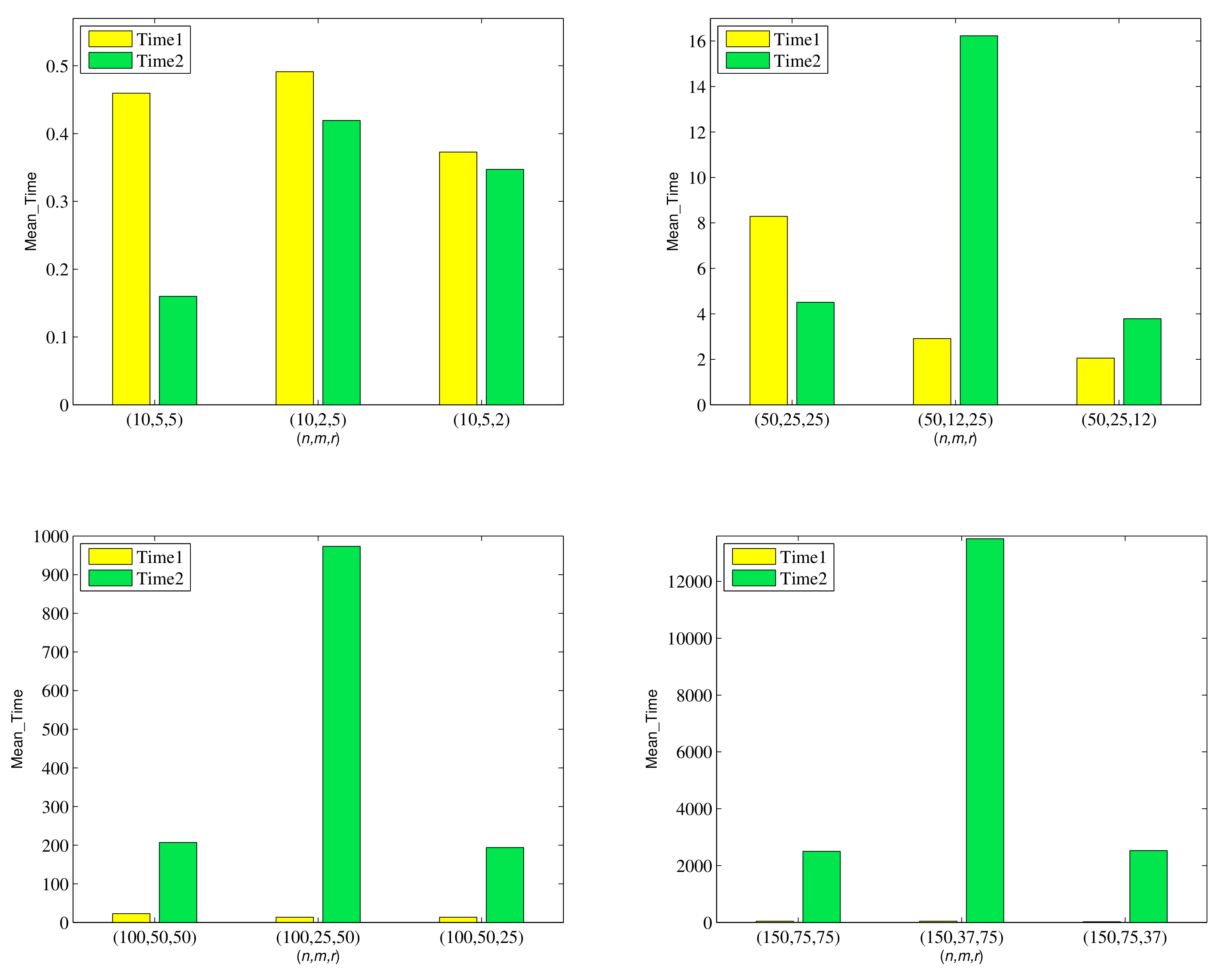
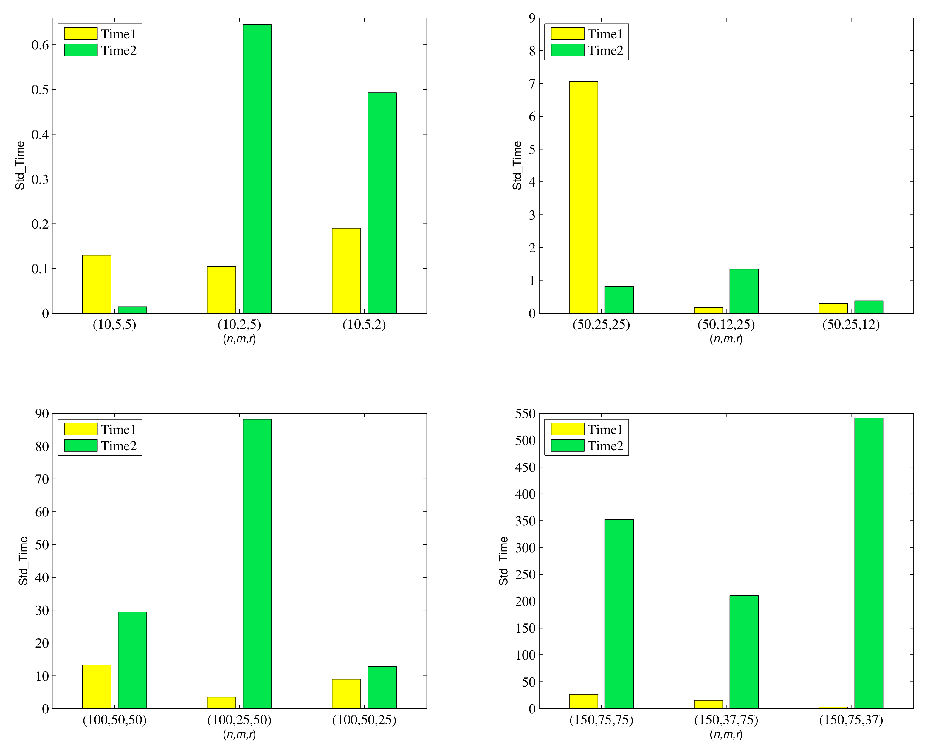
To give an intuitive overview of the results in Table 1, Table 2 and Table 3, we additionally list the following metric comparisons of computing time between the proposed algorithm and the CP relaxation in Figure 3 and Figure 4.
Figure 3 and Figure 4 illustrates that the proposed algorithm provides a better mean value and standard deviation when the dimension n is greater than 100, and the superiority is enlarged when n increases.
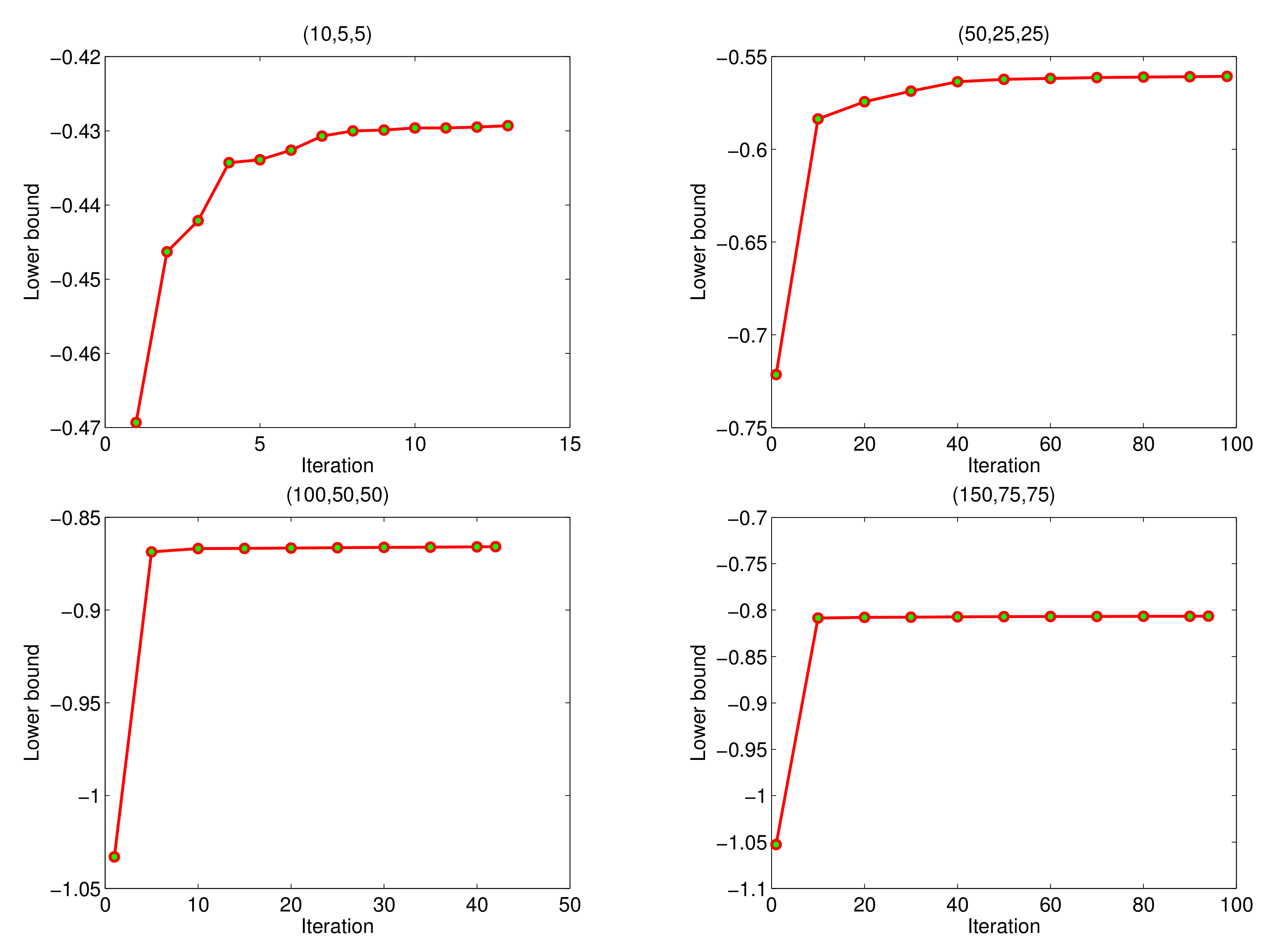
Figure 5 shows the convergence speed of the proposed algorithm. The lower bound updates faster in the first 5 to 10 iterations till it reaches a relatively steady value.
5. Conclusions
We showed that the enhanced SOCP relaxation employing the simultaneous matrix diagonalization technique could result in a better lower bound and reduce the computational complexity compared to the classical SOCP relaxation. Although the lower bound of the enhanced SOCP relaxation is not as good as the copositive relaxation, it benefits from less computational complexity. Numerical experiments imply that the enhanced SOCP relaxation is more suitably applied in the branch and bound algorithm to obtain the optimal solution. For future research, we may focus on designing simultaneous diagonalization-based SOCP relaxation for quadratically constrained quadratic fractional problems.
Author Contributions
Conceptualization, Z.X. and J.Z.; methodology, Z.X. and J.Z.; software, Z.X.; validation, J.Z.; writing—original draft preparation, J.Z.; writing—review and editing, Z.X.; funding acquisition, Z.X. and J.Z. All authors have read and agreed to the published version of the manuscript.
Funding
Xu’s research has been supported by the National Natural Science Foundation of China (Grants #11704336), Zhou’s research has been supported by the National Natural Science Foundation of China (Grant #11701512).
Institutional Review Board Statement
Not applicable.
Informed Consent Statement
Not applicable.
Data Availability Statement
Not applicable.
Conflicts of Interest
The authors declare no conflict of interest.
References
- Lai, H.C.; Huang, T.Y. Optimality conditions for nondifferentiable minimax fractional programming with complex variables. J. Math. Anal. Appl. 2009, 359, 229–239. [Google Scholar] [CrossRef] [Green Version]
- Stancu-Minasian, I.M. Fractional Programming: Theory, Methods and Applications, 1st ed.; Kluwer Academic Publishers: Dordrecht, The Netherlands, 1997; pp. 6–33. [Google Scholar]
- Cai, H.; Wang, Y.; Yi, T. An approach for minimizing a quadratically constrained fractional quadratic problem with application to the communications over wireless channels. Optim. Method Softw. 2014, 29, 310–320. [Google Scholar] [CrossRef]
- Dinkelbach, W. On nonlinear fractional programming. Manag. Sci. 1967, 13, 492–498. [Google Scholar] [CrossRef]
- Salahi, M.; Fallahi, S. On the quadratic fractional optimization with a strictly convex quadratic constraint. Kybernetika 2015, 51, 293–308. [Google Scholar] [CrossRef] [Green Version]
- Zhang, A.; Hayashi, S. Celis-Dennis-Tapia based approach to quadratic fractional programming problems with two quadratic constraints. Numer. Algebra Control Optim. 2011, 1, 83–98. [Google Scholar] [CrossRef]
- Gotoh, J.Y.; Konno, H. Maximization of the ratio of two convex quadratic functions over a polytope. Comput. Optim. Appl. 2001, 20, 43–60. [Google Scholar] [CrossRef]
- Bezdan, T.; Stoean, C.; Namany, A.A.; Bacanin, N.; Rashid, A.T.; Zivkovic, M.; Venkatachalam, K. Hybrid Fruit-Fly Optimization Algorithm with K-Means for Text Document Clustering. Mathematics 2021, 9, 1929. [Google Scholar] [CrossRef]
- Dong, G.; Liu, C.; Liu, D.; Mao, X. Adaptive multi-level search for global optimization: An integrated swarm intelligence-metamodelling technique. Appl. Sci. 2021, 11, 2277. [Google Scholar] [CrossRef]
- Beck, A.; Teboulle, M. A convex optimization approach for minimizing the ratio of indefinite quadratic functions over an ellipsoid. Math. Program. Ser. A 2009, 118, 13–35. [Google Scholar] [CrossRef]
- Xia, Y. Using SeDuMi 1.02, On minimizing the ratio of quadratic functions over an ellipsoid. Optimization 2015, 64, 1097–1106. [Google Scholar] [CrossRef]
- Nguyen, V.B.; Sheu, R.L.; Xia, Y. An SDP approach for quadratic fractional problems with a two-sided quadratic constraint. Optim. Methods Softw. 2016, 31, 701–719. [Google Scholar] [CrossRef]
- Preisig, J.C. Copositivity and the minimization of quadratic functions with nonnegativity and quadratic equality constraints. SIAM J. Control Optim. 1996, 34, 1135–1150. [Google Scholar] [CrossRef]
- Amaral, P.; Bomze, I.M.; Júdice, J. Nonconvex min-max fractional quadratic problems under quadratic constraints: Copositive relaxations. J. Glob. Optim. 2019, 75, 227–245. [Google Scholar] [CrossRef] [Green Version]
- Amaral, P.; Bomze, I.M.; Júdice, J. Copositivity and constrained fractional quadratic problems. Math. Program. 2014, 146, 325–350. [Google Scholar] [CrossRef] [Green Version]
- Sadeghi, A.; Saraj, M.; Amiri, N.M. Solving a fractional program with second order cone constraint. Iran. J. Math. Sci. Inform. 2019, 14, 33–42. [Google Scholar]
- Kim, S.; Kojima, M. Second order cone programming relaxation of nonconvex quadratic optimization problems. Optim. Methods Softw. 2001, 15, 201–224. [Google Scholar] [CrossRef]
- Ben-Tal, A.; Den Hertog, D. Hidden conic quadratic representation of some nonconvex quadratic optimization problems. Math. Program. 2014, 143, 1–29. [Google Scholar] [CrossRef]
- Zhou, J.; Xu, Z. A simultaneous diagonalization based SOCP relaxation for convex quadratic programs with linear complementarity constraints. Optim. Lett. 2017, 13, 1615–1630. [Google Scholar] [CrossRef]
- Zhou, J.; Lu, C.; Tian, Y.; Tang, X. A SOCP relaxation based branch-and-bound method for generalized trust-region subproblem. J. Ind. Manag. Optim. 2021, 17, 151–168. [Google Scholar] [CrossRef] [Green Version]
- Zhou, J.; Chen, S.; Yu, S.; Tian, Y. A simultaneous diagonalization based quadratic convex reformulation for nonconvex quadratically constrained quadratic program. Optimization 2020, in press. [Google Scholar] [CrossRef]
- Liu, X.; Gao, Y.; Zhang, B.; Tian, F. A new global optimization algorithm for a class of linear fractional programming. Mathematics 2019, 7, 867. [Google Scholar] [CrossRef] [Green Version]
- Sturm, J.F. Using SeDuMi 1.02, a MATLAB toolbox for optimization over symmetric cones. Optim. Methods Softw. 1999, 11, 625–653. [Google Scholar] [CrossRef]
Figure 1.
Comparisons of lower bounds and computing time between (6) and (8) with varying dimensions of variables.
Figure 1.
Comparisons of lower bounds and computing time between (6) and (8) with varying dimensions of variables.

Figure 2.
Comparisons of lower bounds and computing time between (6) and (8) with varying numbers of negative eigenvalues of Q.
Figure 2.
Comparisons of lower bounds and computing time between (6) and (8) with varying numbers of negative eigenvalues of Q.

Figure 3.
Mean value of computing times with different sets.

Figure 4.
Standard deviation of computing times with different sets.

Figure 5.
Convergence speed graphs.


Table 1.
Performance Comparisons of the enhanced SOCP relaxation and the CP relaxation with and .
| () | SOCP_BB | CP_BB | ||||
|---|---|---|---|---|---|---|
| LB_SOCP | Opv | Nodes | Time1 | LB_CP | Time2 | |
| (10, 5, 5) | −0.4693 | −0.4293 | 13 | 0.6629 | −0.4293 | 0.1494 |
| (10, 5, 5) | −0.8524 | −0.8456 | 7 | 0.4113 | −0.8456 | 0.1662 |
| (10, 5, 5) | −1.2073 | −1.2021 | 6 | 0.3530 | −1.2021 | 0.1501 |
| (10, 5, 5) | −0.9140 | −0.9072 | 6 | 0.3618 | −0.9072 | 0.1524 |
| (10, 5, 5) | −0.7263 | −0.6881 | 9 | 0.5096 | −0.6881 | 0.1816 |
| (50, 25, 25) | −0.7163 | −0.6067 | 143 | 17.3670 | −0.6067 | 4.5898 |
| (50, 25, 25) | −0.7214 | −0.5607 | 98 | 14.3159 | −0.5607 | 3.6403 |
| (50, 25, 25) | −0.7798 | −0.6902 | 18 | 3.1592 | −0.6902 | 3.7478 |
| (50, 25, 25) | −1.0089 | −0.9433 | 25 | 4.8718 | −0.9433 | 5.0656 |
| (50, 25, 25) | −1.2317 | −1.2083 | 5 | 1.7368 | −1.2083 | 5.4888 |
| (100, 50, 50) | −1.0565 | −0.9001 | 13 | 7.9829 | −0.9001 | 250.9022 |
| (100, 50, 50) | −0.9554 | −0.7997 | 30 | 14.5958 | −0.7997 | 194.6950 |
| (100, 50, 50) | −1.0330 | −0.8659 | 42 | 18.6046 | −0.8659 | 170.7346 |
| (100, 50, 50) | −1.1277 | −0.9654 | 92 | 31.8563 | −0.9654 | 203.0717 |
| (100, 50, 50) | −0.8737 | −0.6899 | 134 | 40.4807 | −0.6899 | 214.5695 |
| (150, 75, 75) | −1.0552 | −0.7857 | 120 | 75.8879 | −0.7857 | 2.7118 × 10³ |
| (150, 75, 75) | −1.1371 | −0.9424 | 14 | 18.4429 | −0.9424 | 2.9627 × 10³ |
| (150, 75, 75) | −1.1903 | −1.0224 | 9 | 17.4320 | −1.0224 | 2.0537 × 10³ |
| (150, 75, 75) | −1.0528 | −0.8065 | 94 | 60.9915 | −0.8065 | 2.4712 × 10³ |
| (150, 75, 75) | −1.2053 | −0.9654 | 38 | 32.4540 | −0.9654 | 2.3078 × 10³ |
| (200, 100, 100) | −1.2726 | −0.9486 | 179 | 187.0444 | - | - |
| (200, 100, 100) | −1.2393 | −0.9090 | 91 | 109.7111 | - | - |
| (200, 100, 100) | −1.1200 | −0.8023 | 499 | 487.9172 | - | - |
| (200, 100, 100) | −1.3677 | −1.0641 | 65 | 80.6285 | - | - |
| (200, 100, 100) | −1.1613 | −0.8508 | 185 | 192.5417 | - | - |
Table 2.
Performance Comparisons of the enhanced SOCP relaxation and the CP relaxation with and .
| () | SOCP_BB | CP | ||||
|---|---|---|---|---|---|---|
| LB_SOCP | Opv | Nodes | Time1 | LB_CP | Time2 | |
| (10, 2, 5) | −0.9896 | −0.9603 | 5 | 0.6060 | −0.9603 | 1.5734 |
| (10, 2, 5) | −0.8272 | −0.7923 | 5 | 0.4432 | −0.7923 | 0.1278 |
| (10, 2, 5) | −0.8851 | −0.8439 | 5 | 0.4632 | −0.8439 | 0.1386 |
| (10, 2, 5) | −1.3820 | −1.3796 | 2 | 0.3577 | −1.3796 | 0.1269 |
| (10, 2, 5) | −1.0857 | −1.0510 | 5 | 0.5859 | −1.0510 | 0.1302 |
| (50, 12, 25) | −1.7140 | −1.6777 | 5 | 3.1569 | −1.6777 | 17.7567 |
| (50, 12, 25) | −1.7958 | −1.7291 | 6 | 2.9847 | −1.7291 | 14.3435 |
| (50, 12, 25) | −1.4860 | −1.3408 | 6 | 2.8456 | −1.3408 | 17.1463 |
| (50, 12, 25) | −1.8775 | −1.7996 | 6 | 2.8528 | −1.7996 | 15.5760 |
| (50, 12, 25) | −1.6074 | −1.5496 | 5 | 2.7021 | −1.5496 | 16.3399 |
| (100, 25, 50) | −1.5728 | −1.3367 | 26 | 19.3778 | −1.3367 | 0.9316 × 10³ |
| (100, 25, 50) | −1.8812 | −1.7798 | 8 | 11.3498 | −1.7798 | 1.0162 × 10³ |
| (100, 25, 50) | −1.7331 | −1.5541 | 8 | 11.3676 | −1.5541 | 1.0123 × 10³ |
| (100, 25, 50) | −2.3014 | −2.2407 | 7 | 12.3799 | −2.2407 | 1.0646 × 10³ |
| (100, 25, 50) | −1.7297 | −1.5881 | 8 | 11.4687 | −1.5881 | 0.8403 × 10³ |
| (150, 37, 75) | −2.2469 | −2.1016 | 8 | 32.4534 | - | - |
| (150, 37, 75) | −2.0106 | −1.7806 | 8 | 32.4796 | - | - |
| (150, 37, 75) | −2.0413 | −1.8458 | 7 | 32.4477 | - | - |
| (150, 37, 75) | −1.8265 | −1.5324 | 41 | 67.4079 | - | - |
| (150, 37, 75) | −1.7998 | −1.5960 | 8 | 36.5955 | - | - |
| (200, 50, 100) | −1.9059 | −1.5500 | 127 | 282.0235 | - | - |
| (200, 50, 100) | −2.0762 | −1.7748 | 8 | 57.7022 | - | - |
| (200, 50, 100) | −1.9991 | −1.6971 | 8 | 55.1303 | - | - |
| (200, 50, 100) | −1.7675 | −1.2039 | 81 | 202.9095 | - | - |
| (200, 50, 100) | −2.0341 | −1.7518 | 9 | 63.0475 | - | - |
Table 3.
Performance Comparisons of the enhanced SOCP relaxation and the CP relaxation with and .
| () | SOCP_BB | CP | ||||
|---|---|---|---|---|---|---|
| LB_SOCP | Opv | Nodes | Time1 | LB_CP | Time2 | |
| (10, 5, 2) | −0.5666 | −0.5666 | 1 | 0.4499 | −0.5666 | 1.2285 |
| (10, 5, 2) | −0.3186 | −0.2993 | 11 | 0.6461 | −0.2993 | 0.1261 |
| (10, 5, 2) | −0.6271 | −0.6271 | 1 | 0.2275 | −0.6271 | 0.1175 |
| (10, 5, 2) | −0.4529 | −0.4509 | 5 | 0.3733 | −0.4509 | 0.1193 |
| (10, 5, 2) | −1.3076 | −1.3076 | 1 | 0.1667 | −1.3076 | 0.1448 |
| (50, 25, 12) | −0.9542 | −0.9241 | 5 | 1.7985 | −0.9241 | 4.0500 |
| (50, 25, 12) | −0.7892 | −0.7576 | 10 | 2.3463 | −0.7576 | 3.4063 |
| (50, 25, 12) | −1.1374 | −1.0829 | 10 | 2.3780 | −1.0829 | 4.0707 |
| (50, 25, 12) | −0.9922 | −0.9727 | 5 | 1.8784 | −0.9727 | 4.0418 |
| (50, 25, 12) | −1.2224 | −1.2045 | 5 | 1.8484 | −1.2045 | 3.3520 |
| (100, 50, 25) | −0.8275 | −0.7157 | 37 | 15.6906 | −0.7157 | 189.7557 |
| (100, 50, 25) | −0.9672 | −0.8460 | 7 | 7.6640 | −0.8460 | 210.9579 |
| (100, 50, 25) | −0.8787 | −0.7226 | 19 | 9.3551 | −0.7226 | 182.1559 |
| (100, 50, 25) | −0.6688 | −0.4729 | 86 | 27.5411 | −0.4729 | 203.2400 |
| (100, 50, 25) | −1.1576 | −1.0850 | 5 | 5.4911 | −1.0850 | 182.8251 |
| (150, 75, 37) | −0.9557 | −0.7539 | 21 | 22.3072 | −0.7539 | 2.2003 × 10³ |
| (150, 75, 37) | −1.0578 | −0.8889 | 9 | 15.3286 | −0.8889 | 2.6835 × 10³ |
| (150, 75, 37) | −1.0882 | −0.8889 | 15 | 19.1659 | −0.8889 | 2.1471 × 10³ |
| (150, 75, 37) | −0.9347 | −0.7677 | 17 | 20.8678 | −0.7677 | 3.4121 × 10³ |
| (150, 75, 37) | −0.9359 | −0.7475 | 24 | 22.9717 | −0.7475 | 2.1899 × 10³ |
| (200, 100, 50) | −0.9704 | −0.7321 | 45 | 67.2220 | - | - |
| (200, 100, 50) | −1.3138 | −1.1077 | 5 | 26.8615 | - | - |
| (200, 100, 50) | −0.9420 | −0.6978 | 158 | 180.3040 | - | - |
| (200, 100, 50) | −0.9998 | −0.7981 | 40 | 62.2748 | - | - |
| (200, 100, 50) | −0.9535 | −0.6954 | 264 | 298.8807 | - | - |
Publisher’s Note: MDPI stays neutral with regard to jurisdictional claims in published maps and institutional affiliations. |
© 2021 by the authors. Licensee MDPI, Basel, Switzerland. This article is an open access article distributed under the terms and conditions of the Creative Commons Attribution (CC BY) license (https://creativecommons.org/licenses/by/4.0/).
Share and Cite
MDPI and ACS Style
Xu, Z.; Zhou, J. A Global Optimization Algorithm for Solving Linearly Constrained Quadratic Fractional Problems. Mathematics 2021, 9, 2981. https://0-doi-org.brum.beds.ac.uk/10.3390/math9222981
AMA Style
Xu Z, Zhou J. A Global Optimization Algorithm for Solving Linearly Constrained Quadratic Fractional Problems. Mathematics. 2021; 9(22):2981. https://0-doi-org.brum.beds.ac.uk/10.3390/math9222981
Chicago/Turabian StyleXu, Zhijun, and Jing Zhou. 2021. "A Global Optimization Algorithm for Solving Linearly Constrained Quadratic Fractional Problems" Mathematics 9, no. 22: 2981. https://0-doi-org.brum.beds.ac.uk/10.3390/math9222981
Note that from the first issue of 2016, this journal uses article numbers instead of page numbers. See further details here.