Efficient or Fractal Market Hypothesis? A Stock Indexes Modelling Using Geometric Brownian Motion and Geometric Fractional Brownian Motion

Abstract

In this article, we propose a test of the dynamics of stock market indexes typical of the US and EU capital markets in order to determine which of the two fundamental hypotheses, efficient market hypothesis (EMH) or fractal market hypothesis (FMH), best describes market behavior. The article’s major goal is to show how to appropriately model return distributions for financial market indexes, specifically which geometric Brownian motion (GBM) and geometric fractional Brownian motion (GFBM) dynamic equations best define the evolution of the S&P 500 and Stoxx Europe 600 stock indexes. Daily stock index data were acquired from the Thomson Reuters Eikon database during a ten-year period, from January 2011 to December 2020. The main contribution of this work is determining whether these markets are efficient (as defined by the EMH), in which case the appropriate stock indexes dynamic equation is the GBM, or fractal (as described by the FMH), in which case the appropriate stock indexes dynamic equation is the GFBM. In this paper, we consider two methods for calculating the Hurst exponent: the rescaled range method (RS) and the periodogram method (PE). To determine which of the dynamics (GBM, GFBM) is more appropriate, we employed the mean absolute percentage error (MAPE) method. The simulation results demonstrate that the GFBM is better suited for forecasting stock market indexes than the GBM when the analyzed markets display fractality. However, while these findings cannot be generalized, they are verisimilar.

1. Introduction

Modeling and forecasting stock price movements has been a key issue in financial studies. In order to make financial and investment decisions, investors use prediction models to assure low investment risk and to have a picture of the market trends. This has inspired a great deal of research into the development and design of prediction models.

The idea of the efficient market, as understood in the modern literature, has its origins in the work of Cootner [1] and Samuelson [2], who postulated the random walk model. The theoretical basis of the efficient market hypothesis (EMH) has to be attributed to the works of Eugene Fama [3,4], which explain the random character of prices as the consequence of rational behaviors.

The EMH theory’s premises can be summarized as follows [5]: (a) investors are rational (in the sense that they correctly update their beliefs about the value of financial securities when new information becomes available in the market); (b) individual investment decisions satisfy the arbitrage condition (arbitrage leads to price equilibrium); and (c) the market is characterized by collective rationality (the different errors in the values of financial securities determined by individual investors cancel each other out in the market). The efficient financial market, according to EMH theory, is the market that fully reflects the available information, and one of the models of the efficient financial market is the random walk model [4]. The random walk model is a financial theory that says that stock market prices cannot be anticipated because they combine the information and expectations of all the market participants. The randomness of prices makes it difficult for investors to outperform the market and earn abnormal returns. Because the EMH is based on standard Brownian motion processes that assume prices evolve through random walk, one obvious consequence is that forecasting future price movements is impossible because market movements are independent and lack autocorrelation, rendering technical analysis useless to investors [6].

The random walk model is a discrete-time model, and the Brownian motion is the continuous-time limit of the discrete-time random evolution. As a result, if the price dynamics of financial securities are described by the geometric Brownian motion (GBM), we can conclude that the market is efficient in the EMH sense. Remember that Norbert Wiener [7] realized the Brownian motion features, which are currently known as the Wiener process.

The efficient market hypothesis (EMH) developed by Fama [3,4], as well as its subsequent extensions, is a vast field of study because the question is whether or not this hypothesis is practicable. However, determining whether a market is efficient is not a straightforward process: a number of works support the EMH [8,9,10,11,12,13,14,15,16], but some studies present arguments in opposition to the EMH [17,18,19]. The majority of the EMH criticism is directed at market participants’ preferences and behavior. Several deviations from the standard EMH paradigm in investor behavior have, therefore, been documented, including over-confidence [20], overreaction [21], herding, and the theory of regret [22]. These EMH critics contend that investors are frequently irrational. From the standpoint of efficiency tests’ applicability, the most significant obstacles of the EMH are the emergence of complex non-linear dynamics and chaos in capital markets [19,23,24,25].

The majority of these empirical studies questioned the rationality and absence of memory in asset prices. The interest in market finance in the study of memory processes stems from the fact that it is seen as a viable alternative to testing the efficient market hypothesis in a very easy manner. Many recent studies have looked into the long-term memory of asset returns, demonstrating that prices reflect a fractional Brownian motion [23,26,27,28,29,30,31,32,33,34,35,36,37]. In general, if a title has long-term memory, it may be argued that it has cyclical behavior and, therefore, does not follow a random process, which would directly contradict the efficiency hypothesis. However, as others [38] point out, this approach is far from simple since additional factors must be taken into account when drawing results. Furthermore, other researchers have concluded that there is no strong evidence for long-term memory in common stock returns [39,40].

Based on the idea of using the fractional Brownian motion instead of the Brownian motion, the stock price could be examined utilizing fractal properties. The fractal Brownian motion, first proposed by Mandelbrot and Van Ness [41], is used to simulate different fractal noises. It has evolved into a mathematical model that can reflect the properties of a wide range of natural objects.

The fractal market hypothesis (FMH) was proposed by Edgar E. Peters [42] as a feasible instrumental alternative to the EMH. While the EMH assumes that financial markets are in equilibrium, the FMH assumes that financial markets are not in equilibrium but can be stable, which is achieved by investors covering a large number of investment horizons. Unlike the EMH, the FMH asserts that market information is valued by investors according to their investment horizons. At any point in time, prices may not reflect all the available information but only information for one investment horizon.

The FMH’s premises can be summarized as follows [42]: (a) the financial market is stable if investors cover a wide range of investment horizons; (b) the information set is influenced by short-term factors and market sentiment, with fundamental information dominating in the long term; (c) if a market event casts doubt on fundamental information, long-term investors will trade on short-term information; (d) prices reflect a combination of technical and fundamental analysis; (e) a financial security is not related to the economic cycle; there will be no long-term trend.

The FMH highlights the impact of liquidity and the starting point of investment de-pending on investor behavior. Its goal is to provide a model of investor behavior and market price movement in accordance with investor expectations [43]. The FMH relaxes the EMH Brownian motion requirement of financial securities and posits that price movements follow fractional Brownian motion, as measured by the Hurst exponent. The Hurst exponent affects whether a fractal time series evolves by a random walk, a persistent trend, or mean reversion. If the movement of stock market indexes can be explained using geometric fractional Brownian motion (GFBM), it is possible to conclude that the market is unpredictable, inefficient, and fractal in the sense of FMH.

Osborne [44], an American astronomer, published his hypothesis that price follows a geometric Brownian motion—the distribution of price changes is log-normal—in the late 1950s. To represent the behavior of risky asset values, Black and Scholes [45], Scholes [46], and Merton [47] advocated using a Brownian motion method. Since then, authors have used the GBM to simulate stock price pathways and examine whether the simulated stock prices match the actual market returns [48,49]. While the majority of these studies focus on stock prices, others have discovered that commodity prices, such as crude palm oil [50], petroleum products and natural gas [51], gold [52], and other commodities, exhibit randomness that can be explained mathematically using the GBM model.

To address the major flaw in GBM modeling, which assumes real stock increments to be mutually independent, fractional Brownian motion was introduced by Andrey Kol-mogorov [53], but the first mathematical definition and properties of this stochastic process were given by Mandelbrot and Van Ness [41] by incorporating the Hurst exponent in stock price dynamics to improve the accuracy of stock price modeling by providing information on the level of self-similarity in a given time series. We mention also the contributions of Mandelbrot with Wallis [54,55,56,57], who introduced the concepts of fractional Gaussian noises and fractional Brownian motion and related these to R/S analysis.

Geometric fractional Brownian motion has been studied extensively, with many studies identifying potential applications in the context of neuronal models [58]. It was validated by a rigorous statistical test with added white Gaussian noise based on the autocovariance function [59] and has been applied in studies both for stock indexes [60] and for the price of financial securities [61], in the case of cryptocurrencies [62], in the case of modeling epidemic diseases, such as coronavirus [63], and for the price of goods [50]. Furthermore, the GFBM has been utilized in a great deal of literature research to evaluate derivative titles (options) [64,65,66,67].

The authors of several more recent research studies have proposed a number of GFBM extensions and adjustments, including the fractional Brownian motion model with adaptive parameters [68], irrational fractional Brownian motion model [69], fractional Brownian motion with two-variable Hurst exponent [70], or approximate fractional Brownian motion [71].

The primary aim of the article is to demonstrate how to properly model return distributions for financial market indexes. Because the efficient market hypothesis does not fully characterize financial market behavior, we investigate if a different method—the fractal markets hypothesis—yields more accurate results.

In this article, we will test which of the dynamics equations, represented by geometric Brownian motion (GBM) and geometric fractional Brownian motion (GFBM), best de-scribes the evolution of the S&P 500 and Stoxx Europe 600 stock indexes for the US market and the EU market, respectively. The main contribution of this paper is to determine whether these markets are efficient (as defined by the efficient market hypothesis), in which case the appropriate dynamics equation of stock indexes is the GBM, or fractal (as defined by the fractal market hypothesis), in which case the appropriate dynamics equation of stock indexes is the GFBM. The aim of this paper is to highlight the practical implications of our findings on the capital markets under consideration. Because information is viewed as a generic item in classical finance theory, the EMH implies that various information affects investors in the same way. Furthermore, the FMH claims that information is valued based on each investor’s time horizon. As a result, information has a varied value for each investor group, and each has its own set of trading rules and tactics. Indeed, while traders are mostly concerned with the short term, investors are primarily concerned with long-term investments.

Ibrahim, Misiran, and Laham [50] conducted similar analyses but on commodity price modeling. Moreover, in a recent study of 26 international stock market indexes, Dittrich and Srbek [72] concluded that Brownian motion cannot be perceived as a norm for describing stock market behavior, challenging the assumption of a random walk of stock prices. This paper is one of the few that performs EMH and FMH tests utilizing dynamics equations represented by GBM and GFBM rather than the traditional testing methods in which the Hurst index is calculated but the dynamics of evolution are not determined; therefore, predictions cannot be made. Such predictions on the evolution of stock indexes using dynamics equations become possible with our technique.

The R/S analysis, established by Mandelbrot and Wallis [54], is the most common of the various methodologies developed to get a numerical value of the Hurst exponent. The lack of a distribution theory for the underlying statistic, as well as its sensitivity to the presence of explicit short-range dependence structures, make the standard R/S analysis less appealing. Authors, such as Lo [17], and, more recently, others, such as Sánchez-Granero et al. [19] or Weron [73], have shown that, when the length of the time series is too short, the resultant value for the exponent is far from acceptable, emphasizing the difficulty in the case of financial series. While classical R/S analysis is not very reliable in the presence of small samples, it can be very effective and useful as a graphical method in the presence of reasonably large samples, where it often provides a fairly accurate picture of the presence or absence of long-range dependence in a given empirical record, and, in the former case, about the intensity of long-range dependence as measured by the Hurst parameter. The most beneficial aspect of the classical R/S analysis for practical purposes is its relative robustness to changes in the marginal distribution of the data, even if the marginals contain heavy tails with infinite variance (see, for example, ref.[54,74,75]).

As a result, one of the main lines of research is on refining and improving the Hurst exponent estimating procedures, either through improved R/S analysis [17,73] or the invention of new methodologies, such as the ones described as follows: the log-periodogram estimator (the GPH estimator of Geweke and Porter-Hudak [76]), the quasi maximo likelihood model (QML) [77], the generalized Hurst exponent (GHE) [78], the periodogram method (PE) [79], the wavelets methodology [80], the centered moving average method (CMA) [81], the MF-DFA methodologies [82], geometric method-based procedures (GM) [19], and, more recently, the fractal dimension algorithm (FD) [83], the total triangles area algorithm (TTA) [84], the wavelet analysis [85,86,87], or the local Whittle’s estimation [88].

In this paper, we first consider the rescaled range method (RS) for calculating the Hurst exponent. However, due of the criticism aimed at this approach’s imprecision (its sensitivity to the presence of explicit short-range dependence structures), we chose the periodogram method (PE) as an alternative. To determine which of the dynamics (GBM, GFBM) is more appropriate, we employed the mean absolute percentage error (MAPE) method.

To preview our findings, the GFBM model outperforms the GBM model in forecasting future price patterns for the dataset presented. The S&P 500 and Stoxx Eur 600 stock indexes follow a GFBM, according to our analysis, across 3-, 5-, 7-, and 10-year time periods, utilizing values of the Hurst exponent determined using the PE approach, so the US and EU equity markets can be called fractal markets. This conclusion holds true even when the Hurst exponent is generated using the RS approach for the S&P 500 stock index. However, using the GFBM to derive the Hurst exponent produces reasonable forecasts for the Stoxx Eur 600 index, with the exception of the 3-year period, where the forecast is considered good. The latter circumstance is also observed when the Hurst exponent is assumed to be 0.5, in which case the GBM provides the dynamics of the Stoxx Eur 600 index. What can be seen is that the PE technique results for Hurst show that the series are anti-persistent much more clearly, which justifies the GFBM.

This article is organized as follows. Section 2 follows the introduction and discusses the research methodology used in this study, as well as the mathematical models applied to the indexes, geometric Brownian motion (GBM), geometric fractional Brownian motion (GFBM), Hurst index (H), and mean absolute percentage error (MAPE). The empirical findings and discussion are reported in Section 3. The study’s conclusions are summarized in the final section of the article.

2. Research Methodology

In the following, we describe the mathematical models geometric Brownian motion (GBM) and geometric fractional Brownian motion (GFBM) applied to stock market indexes, Hurst index (H), and mean absolute percentage error (MAPE). The latter will be used as a predictability metric in our investigation. In other words, we will use the MAPE tool to assess which of the two dynamics models best describes the evolution of the values of the stock market indexes under consideration.

2.1. Geometric Brownian Motion (GBM)

Geometric Brownian motion and geometric fractional Brownian motion (GFBM) imply that the change in the logarithm of the stock index value is a random variable.

Definition 1.

Let SI be the value of the stock market index,$t\in \left(0,T\right)$the time moment, T the total time, and$\Delta t=\frac{1}{T}$the time lag. Then, the logarithmic return$R\left(t\right)$of SI in the time interval$\left(t,t+\Delta t\right)$is

$$R\left(t\right)=ln\frac{SI\left(t+\Delta t\right)}{SI\left(t\right)}=lnSI\left(t+\Delta t\right)-lnSI\left(t\right)=\Delta lnSI.$$

(1)

Definition 2.

A stochastic process$\left\{B\left(t\right), t\ge 0\right\}$is a standard Brownian motion (BM) if it satisfies the following three conditions:

1. 

For any moments of time$0\le t_1\le t_2\le \dots t_{n-1}\le t_n$, the increments$B\left(t_2\right)-B\left(t_1\right),\dots ,B\left(t_n\right)-B\left(t_{n-1}\right)$are independent;

2. 

Each increment is a Gaussian random variable of zero mean and variance t − s, so:$B\left(t\right)-B\left(s\right)~N\left(0,t-s\right)$,$\forall s<t;$

3. 

B(0) = 0.

A real-valued stochastic process${\left(X_t\right)}_{t\ge 0}$is a Markov process if for all Borel set$A\subset ℝ$and all real numbers$t>s>0$,$P\left(X_t\in A|X_u, u\le s\right)=P\left(X_t\in A|X_s\right)$.

A Brownian motion$\left\{B\left(t\right), t\ge 0\right\}$is a Markov process [89].

According to Negrea [90], the main properties of BM are:

• BM trajectories are continuous and not derivable;
• Stochastic processes$\left\{B\left(t\right), t\ge 0\right\}$, and$\left\{B^2\left(t\right)-t;t\ge 0\right\}$are martingale, and, reciprocally, if$SI\left(t\right)$is a continuous process such that$SI\left(t\right)$and ($S{I}^2\left(t\right)-t, t\ge 0)$are martingale, then$SI\left(t\right)$is a BM;
• Stochastic process$\left\{e^{\left[\lambda B\left(t\right)-\frac{1}{2}{\lambda }^{2}t\right]}, t\ge 0\right\}$is a martingale for any$\lambda$real and reciprocally. If$SI\left(t\right)$is a continuous process such that$\left\{e^{\left[\lambda SI\left(t\right)-\frac{1}{2}{\lambda }^{2}t\right]}, t\ge 0\right\}$is a martingale for any$\lambda$real, then$SI\left(t\right)$is a Brownian motion.

Definition 3.

A stochastic process$\left\{SI\left(t\right), t\ge 0\right\}$follows a geometric Brownian motion (GBM) if the value of the stock index is described by the following dynamics equation

$$dSI\left(t\right)=\mu SI\left(t\right)dt+\sigma SI\left(t\right)dB\left(t\right)$$

(2)

where$\mu$is the drift coefficient, $\sigma$is the diffusion coefficient,$dB$is the infinitesimal variation of a standard Brownian.

Using the stock index’s dynamics equation$dSI\left(t\right)=\mu SI\left(t\right)dt+\sigma SI\left(t\right)dB\left(t\right)$and applying the Itô lemma, it follows

$$dlnSI=\left(\mu -\frac{1}{2}{\sigma }^2\right)dt+\sigma dB\left(t\right).$$

(3)

By integrating Equation (3), we obtain

$$lnSI\left(t\right)=lnSI\left(0\right)+ln{e}^{\left[\underset{0}{\overset{t}{{\displaystyle \int }}}\left(\mu -\frac{1}{2}{\sigma }^2\right)ds+\underset{0}{\overset{t}{{\displaystyle \int }}}\sigma dB\left(s\right)\right]},$$

(4)

where $SI\left(0\right)$is the initial value of the stock market index and$SI\left(t\right)$is the value of the stock market index at time t in the future.

Equation (4) can also be written as

$$SI\left(t\right)=SI\left(0\right)e^{\left[\mu t-\frac{1}{2}{\sigma }^{2}t+\sigma B\left(t\right)\right]}$$

(5)

equivalent

$$ln\frac{SI\left(t\right)}{SI\left(0\right)}=\left[\mu t-\frac{1}{2}{\sigma }^{2}t+\sigma B\left(t\right)\right].$$

(6)

Or, over a time lag, the solution is

$$SI\left(t+\Delta t\right)=SI\left(t\right)\exp \left\{\left(\mu -\frac{1}{2}{\sigma }^2\right)\Delta t+\sigma \left[B\left(t+\Delta t\right)-B\left(t\right)\right]\right\}$$

(7)

where$B\left(t+\Delta t\right)-B\left(t\right)~N\left(0,\Delta t\right).$

Further, from Equation (7), the logarithmic return of the stock market index modelled by a GBM for a time lag$\left(\Delta t\right)$can be written as follows

$$\Delta lnSI=R\left(t\right)=\left(\mu -\frac{1}{2}{\sigma }^2\right)\Delta t+\sigma \left[B\left(t+\Delta t\right)-B\left(t\right)\right]$$

(8)

with$t\ge 0$.

Moreover, given that$B\left(t+\Delta t\right)-B\left(t\right)~N\left(0,\Delta t\right)$the logarithmic distribution of the stock index return modelled by a GBM can be written as follows:

$$R\left(t\right)~N\left[\left(\mu -\frac{1}{2}{\sigma }^2\right)\Delta t,\sigma \sqrt{\Delta t}\right].$$

(9)

2.2. Geometric Fractional Brownian Motion (GFBM)

Definition 4.

A stochastic process$\left\{B_H\left(t\right), t\ge 0\right\}$is a fractional Brownian motion (FBM) if it satisfies the following three conditions:

1. 

is a centered Gaussian process,$E\left[B_H\left(t\right)\right]=0, \forall t\ge 0$;

2. 

the autocovariance of the increments is given by

$$Cov\left[B_H\left(t\right),B_H\left(s\right)\right]=E\left(B_H\left(t\right)\Delta B_H\left(s\right)\right)=\frac{1}{2}\left({\left|t\right|}^{2H}+{\left|s\right|}^{2H}-{\left|t-s\right|}^{2H}\right), t,s\ge 0, H\in \left(0,1\right);$$

(10)

3. 

$B_H\left(0\right)=0$.

If$H=\frac{1}{2}$, FBM is a BM, in which case the increments are independent.

It is known that a fractional Brownian motion is not a Markov process [91,92].

The main properties of FBM are [93]:

• $\forall a, a>0,$stochastic process$\left\{a^{-H}{B}_H\left(at\right), t\ge 0\right\}$is an FBM with Hurst parameter (self-similarity property);
• $\forall s,t, 0\le s<t$, the increments of the process$B_H\left(t\right)-B_H\left(S\right)$have a Gaussian distribution of zero mean and variance${\left|t-s\right|}^{2H}$(stationarity property of the increments);$\forall n$and$\forall t_i$,$t_i=1,\dots ,n$, for each time instant$0\le t_1\le t_2\le \dots t_{n-1}\le t_n$, the increments$B\left(t_2\right)-B\left(t_2\right)\dots B\left(t_n\right)-B\left(t_{n-1}\right)$are not independent (the non-independence property of increments); the stochastic process$\left\{B_H\left(t\right), t\ge 0\right\}$has continuous trajectories, i.e., there is a$C>0$such that:

  $$\underset{s\le t}{sup}\left|B_t^H\left(\omega \right)-B_s^H\left(\omega \right)\right|\le C{\left|t-s\right|}^{\alpha }$$

  for$\alpha \in \left(0,H\right)$(property$\alpha$—Hölder continuous sample paths); stochastic process$\left\{B_H\left(t\right), t\ge 0\right\}$does not admit derivative with respect to time (property of no differentiable sample paths); stochastic process$\left\{B_H\left(t\right), t\ge 0\right\}$is not a semimartingale, except for$H=\frac{1}{2}$(no semimartingale property).

In quantitative finance, geometric fractional Brownian motion (GFBM), also called geometric fractal Brownian motion, is a generalization of GBM, in which$B\left(t\right)$becomes$B_H\left(t\right)$, the increments are not independent, and$B_H\left(t\right)$is obtained as follows [41]:

$$B_H\left(t\right)= \frac{1}{\Gamma \left(H+\frac{1}{2}\right)}\left[Z\left(t\right)+{{\displaystyle \int }}_0^t{\left(t-s\right)}^{H-\frac{1}{2}} dB\left(s\right)\right],$$

(11)

where$B_H\left(t\right)$is a fractional Brownian motion,$\Gamma$is the gamma function,$H\in \left(0,1\right)$is the Hurst exponent, and

$$Z\left(t\right)={{\displaystyle \int }}_{-\infty }^0{\left(t-s\right)}^{H-\frac{1}{2}}-{\left(-s\right)}^{H-\frac{1}{2}} dB\left(s\right)$$

(12)

Definition 5.

A stochastic process$\left\{S{I}_H\left(t\right), t\ge 0\right\}$follows a geometric fractional Brownian motion (GFBM) if the value of the stock index is described by the following dynamics equation:

$$dS{I}_H\left(t\right)=\mu S{I}_H\left(t\right)+\sigma SI\left(t\right)d{B}_H\left(t\right).$$

(13)

Integrating Equation (13), which is based on a Wick product renormalization operator [94], yields:

$$S{I}_H\left(t\right)=S{I}_H\left(0\right)e^{\left[\mu t-\frac{1}{2}{\sigma }^2{t}^{2H}+\sigma B_H\left(t\right)\right]},$$

(14)

equivalent

$$ln\frac{S{I}_H\left(t\right)}{S{I}_H\left(0\right)}=\left[\mu t-\frac{1}{2}{\sigma }^2{t}^{2H}+\sigma B_H\left(t\right)\right].$$

(15)

Or, over a time lag, the solution is [95]:

$$S{I}_H\left(t+\Delta t\right)=S{I}_H\left(t\right)exp\left\{\left(\mu -\frac{1}{2}{\sigma }^2\right)\Delta t+\sigma \left[B_H\left(t+\Delta t\right)-B_H\left(t\right)\right]\right\},$$

(16)

where

$$B_H\left(t+\Delta t\right)-B_H\left(t\right)~N\left(0,{\left|\Delta t\right|}^{2H}\right)$$

(17)

Further, from Equation (16), the logarithmic return of the stock index modelled by an FGBM for a time lag$\left(\Delta t\right)$can be written as follows:

$$\Delta lnS{I}_H=R_H\left(t\right)=\left(\mu -\frac{1}{2}{\sigma }^2\right)\Delta t+\sigma \left[B_H\left(t+\Delta t\right)-B_H\left(t\right)\right],$$

(18)

with$t\ge 0$.

It should be noted that the increments

$$X_H\left(t\right)\Delta B_H\left(t+\Delta t\right)-B_H(t)$$

(19)

are referred to as fractional Gaussian noise (FGN) in the time interval$\Delta t$, being in fact an incremental process of the GFBM, and may be computed by an exact approach known as Cholesky decomposition. Detailed expositions of this method can be found in Feng [95] or Kijima and Tam [96].

From (18), we get$E\left[R_H\left(t\right)\right]=\left(\mu -\frac{1}{2}{\sigma }^2\right)\Delta t$.

By elementary calculations, it can be obtained$Var\left(R_H\left(t\right)\right)={\sigma }^2{\left|\Delta t\right|}^{2H}.$

Therefore,

$$R_H\left(t\right)~N\left[\left(\mu -\frac{1}{2}{\sigma }^2\right)\Delta t,\sigma \sqrt{{\left|\Delta t\right|}^{2H}}\right]$$

(20)

From (18) and (20), we get

$$\frac{R_H\left(t\right)-E\left[R_H\left(t\right)\right]}{\sqrt{Var\left[R_H\left(t\right)\right]}}=\frac{X_H\left(t\right)}{{\left|\Delta t\right|}^H}$$

From the above relation, it can be noted that the standardization of the logarithmic stock index return in the GFBM is a rescaled FGN.

By elementary calculations, the autocovariance of FGN with lag$\tau$can be obtained as follows:$c_H\left(\tau \right)=Cov\left(X_H\left(t+\tau \right),X_H\left(t\right)\right)=\frac{1}{2}\left({\left|\tau -\Delta t\right|}^{2H}-2{\left|\tau \right|}^{2H}+{\left|\tau +\Delta t\right|}^{2H}\right)$.

Considering a series of logarithmic returns$\left\{R_H\left(t_k\right), k=1,\dots ,n\right\},$denote thesample mean by$M\left(R\right)=\frac{1}{n}{\displaystyle \sum }_{k=1}^n{R}_H\left(t_k\right)$andsample variance by${\sigma }^2\left(R\right)=\frac{1}{n-1}{\displaystyle \sum }_{k=1}^n{\left(R_H\left(t_k\right)-M\left(R\right)\right)}^2$.

Using relation (20), the volatility and the drift of stock returns can be estimated as follows:$\tilde{\sigma }\Delta \sqrt{\frac{{\sigma }^2\left(R\right)}{{\left|\Delta t\right|}^{2H}}}$,$\tilde{\mu }\Delta \frac{M\left(R\right)}{\Delta t}+\frac{{\tilde{\sigma }}^2}{2}$.

As we can see from the above, GFBM requires determining the value of the Hurst exponent, which, depending on its size, can explain three situations:

1. 

if$H\in \left(0,\frac{1}{2}\right)$, this situation implies that the FBM increments are negatively correlated, which means that the process is anti-persistent (the process is mean-reverting);

2. 

if$H=\frac{1}{2}$, this implies that the FBM increments are independent, which means that the process is a BM or Wiener process;

3. 

if$H\in \left(\frac{1}{2},1\right)$, this implies that the FBM increments are positively correlated, suggesting that the process is persistent.

2.3. Hurst

Many articles have proposed methods for estimating the Hurst exponent H of fGn. A summary of these methods is given by [97]. In our study, we look at two approaches for estimating the Hurst exponent: the rescaled range method (RS) (a method used in the time domain), and the periodogram method (PE) (in the frequency domain). In the following, we will make a short presentation of these two methods.

The Hurst exponent calculating methods will be presented in the following sections.

2.3.1. Rescaled Range (RS) Computation Methodology

The most known methodology to give the Hurst exponent is RS analysis, introduced by Mandelbrot and Wallis in 1968 [54]. In practice, classical RS analysis is based on a heuristic graphical approach that attempts to exploit as fully as possible the information in a given historical record.

For a time series of length m and for each $n=2^k<m$, we divide the series into $N=\frac{m}{n}$ non-overlopping blocks of length $n$.

Let $m_i$ the mean and $S_i$ the standard deviation of each block $X=\left\{X_1,X_2,\cdots ,X_n\right\},i=1,2,\cdots ,N$.

The data of each block $X_i$ are normalized as follows: $N_j=X_j-m_i, j=1,\cdots ,n.$

Let $C_j, j=1,\cdots ,N$ the cumulative series for each block. Denote $R_i=max\left\{C_j, j=1,\cdots ,n\right\}-min\left\{C_j, j=1,\cdots ,n\right\},$the range of $C_j$ for each block.

The new sequence ${\left(\frac{R_i}{S_i}\right)}_{i=1,\cdots ,N}$ is called rescaled range deviation. Consider $R{S}_m=\frac{1}{N}{\displaystyle \sum }_{i=1}^N\frac{R_i}{S_i}$ the average of the range change.

The slope of the linear regression of $\log \left(R{S}_m\right)$ and $\log n$can be used to determine the Hurst exponent.

For this methodology, the readers are directed to the sources [98,99].

2.3.2. Periodogram Method (PE)

The first presentation of the periodogram method was elaborated by Geweke and Porter-Hudak [76], who presented a very important work on stationary long memory processes. Their paper gave rise to several other works and presented a proof for the asymptotic distribution of the long memory parameter. The periodogram method is based on Fourier transform [23]. Using the concept of FGN described in the previous section, in the following, we will present PE method to calculate the Hurst exponent.

From [97], the spectral density of an FGN defined in (19) can be written as:

$$S\left(f\right)={{\displaystyle \sum }}_{\tau =-\infty }^{\infty }{e}^{-2\pi if\tau }{c}_H\left(\tau \right)=4{\sigma }^2{C}_{H}si{n}^2\left(\pi f\right){{\displaystyle \sum }}_{j=-\infty }^{\infty }\frac{1}{{\left|f+j\right|}^{2H+1}},-\frac{1}{2}\le f\le \frac{1}{2},$$

(21)

where $c_H\left(\tau \right)$ is the autocovariance function of the FGN with $lag \tau$ and ${\Delta }_t=1$ and

$$C_H=\frac{\Gamma \left(2H+1\right)\sin \left(\pi H\right)}{{\left(2\pi \right)}^{2H+1}} .$$

(22)

Using Taylor formula, we get

$$S\left(f\right)\approx {\sigma }^2{C}_H{\left(2\pi \right)}^2{\left|f\right|}^{\gamma },-\frac{1}{2}\le f\le \frac{1}{2},$$

(23)

where $\gamma =1-2H$.

Let $\left(x\left(t_1\right),\cdots ,x\left(t_n\right)\right)’$ be a sequence of a time series $\left\{X\left(t\right),t\ge 0\right\}$ and $\widehat{\mu }=\frac{1}{n}{\displaystyle \sum }_{i=1}^{n}x\left(t_i\right).$

We consider the following estimate of the spectral density (see [95])

$$\widehat{S}\left(f\right)=\frac{1}{n}{\left|{{\displaystyle \sum }}_{\tau =0}^{n-1}\left[x\left(\tau \right)-\widehat{\mu }\right]e^{-2i\pi f\tau }\right|}^2,-\frac{1}{2}\le f\le \frac{1}{2}.$$

(24)

For the frequencies up to the size $N^{\frac{4}{5}}$, we have $\widehat{S}\left(f\right)~{\left|f\right|}^{\gamma }$.

From relation (23), we get $ln\widehat{S}\left(f\right)\approx ln{\sigma }^2{C}_H{\left(2\pi \right)}^2+\gamma \ln \left|f\right|.$

So, the estimate of the Hurst exponent H can be obtained by the slope of linear regression of $ln\widehat{S}\left(f\right)$ and $\ln \left|f\right|$.

2.4. Mean Absolute Percentage Error (MAPE)

The GMB and GFBM models for the stock market indexes we study can be evaluated using mean absolute percentage error (MAPE). In reality, we use this tool to assess the accuracy of forecasting the value of stock market indexes using the GBM and GFBM dynamics equations, respectively.

The use of the MAPE method in validating forecast models is one of the most widely used measures of forecast accuracy, obviously subject to falsification in the sense of Popper [100,101].

Formally, the MAPE expression is:

$$MAPE=\frac{1}{n}{{\displaystyle \sum }}_{t=1}^n\left|\frac{S{I}_A\left(t\right)-S{I}_F\left(t\right)}{S{I}_{A\left(t\right)}}\right|\times 100,$$

(25)

where $S{I}_A\left(t\right)$ is the real value of the stock market index; $S{I}_F\left(t\right)$ is the forecast value of the stock market index; n is the total number of forecasts.

Table 1. Mean absolute percentage error (MAPE) values and interpretation.

MAPE Value	Interpretation
<10%	Highly accurate forecasting
10–20%	Good forecasting
20–50%	Reasonable forecasting
>50%	Inaccurate forecasting

Source: Azizah et al. [47].

shows the interpretation of the result acquired with MAPE.

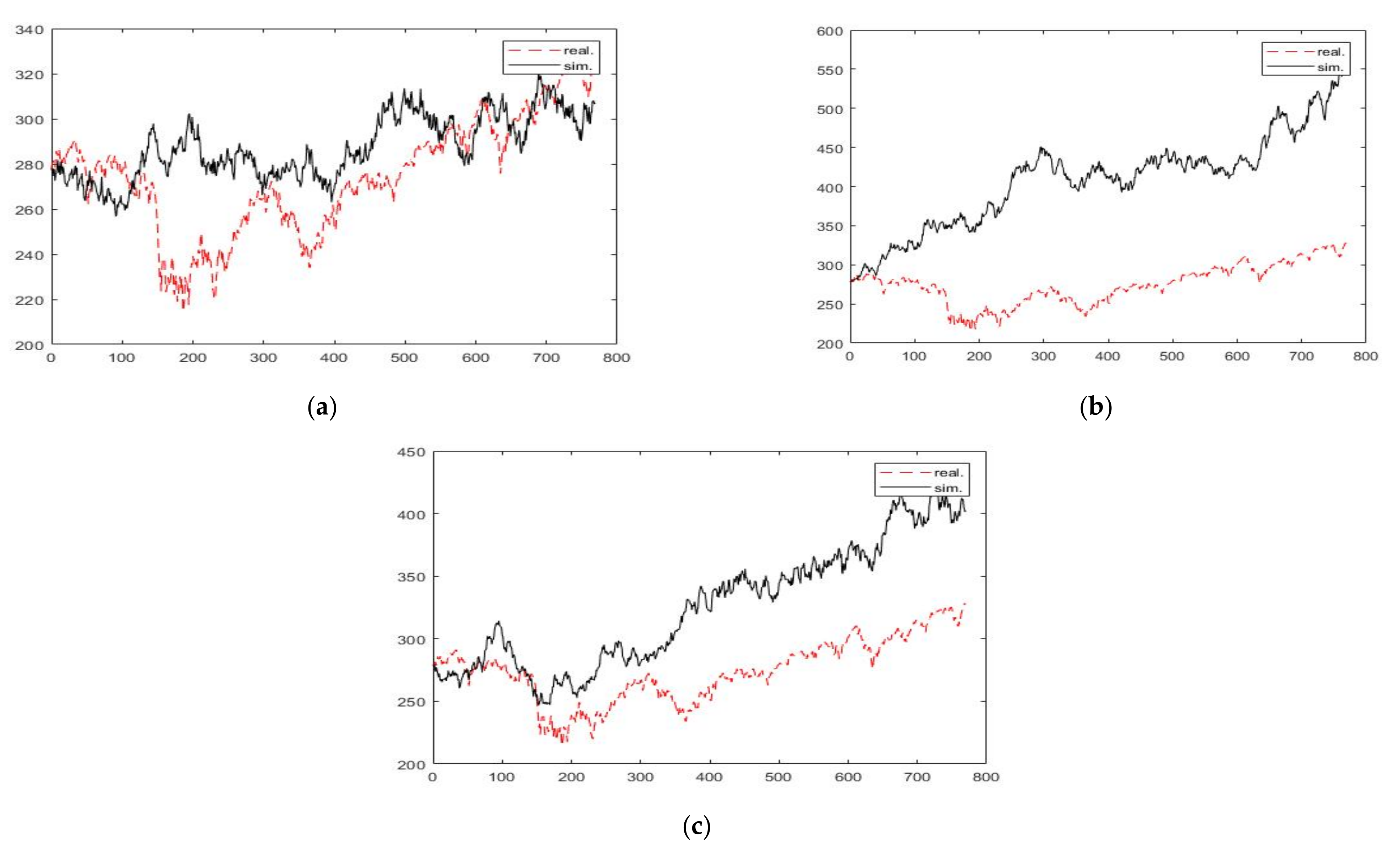
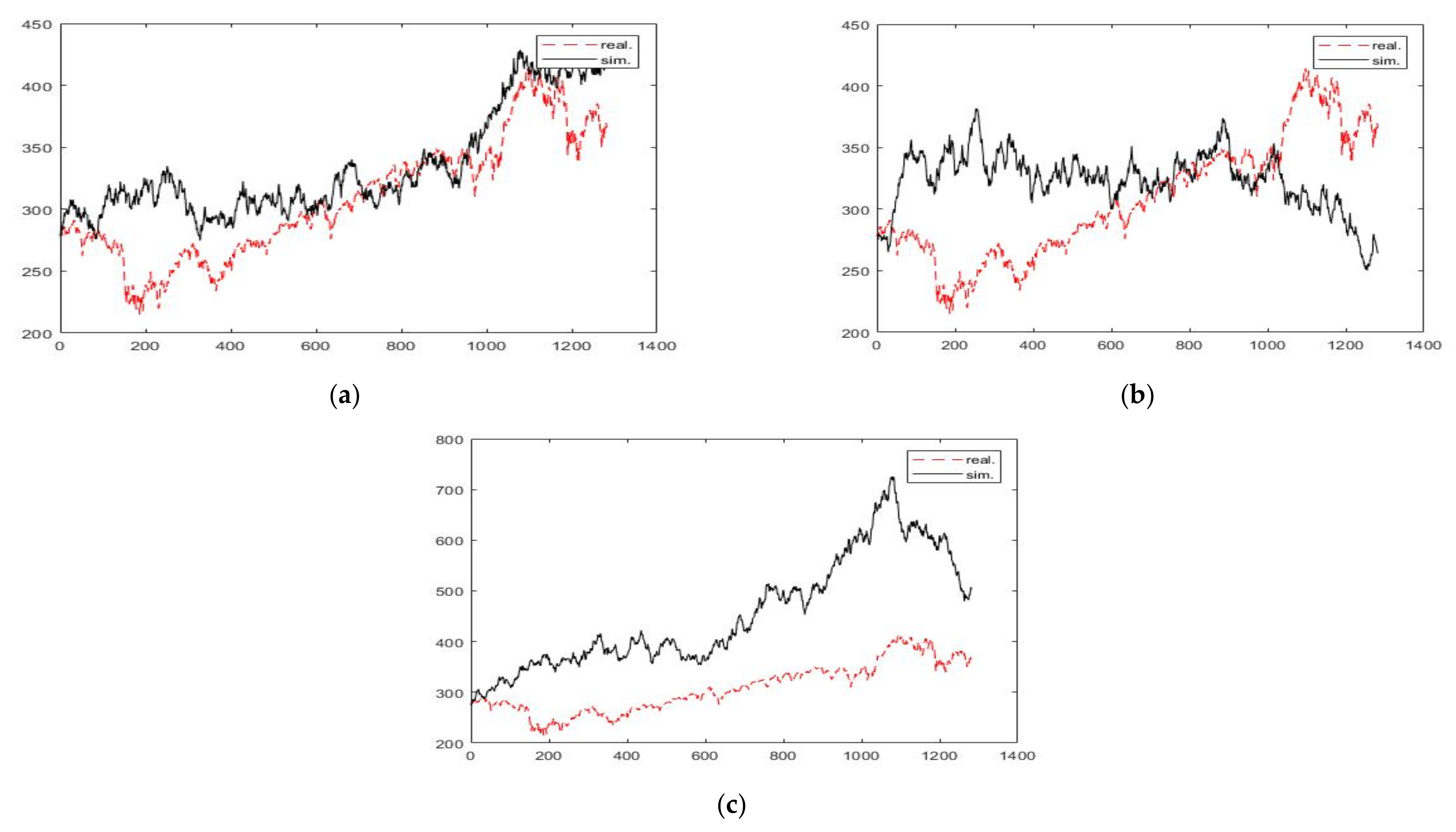
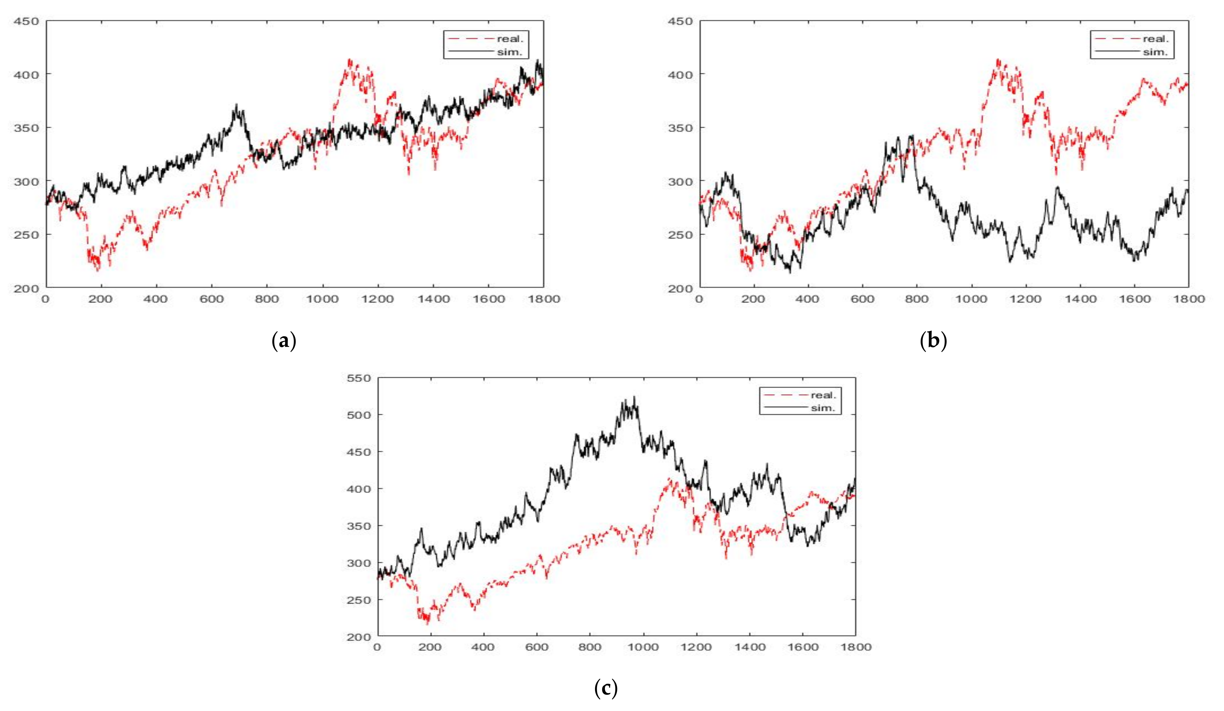
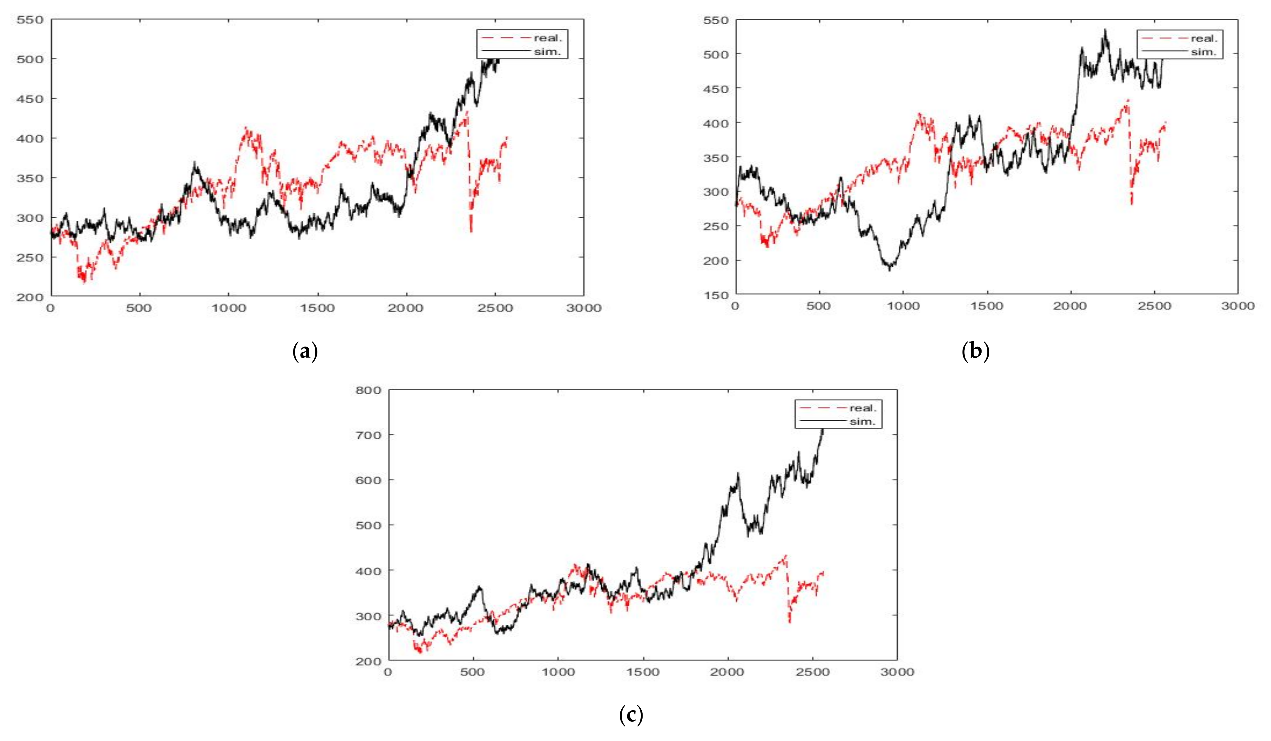
3. Results and Discussion

In the following section, based on the methodology presented above, we will analyze the dynamics of the S&P 500 and Stoxx Europe 600 stock market indexes, representing the US market and the EU market, respectively. The two stock market indexes used to evaluate the efficiency or fractality of the two markets are considered representative indexes since they can accurately define both markets.

In this regard, our analysis takes a 10-year period into account, with the following sub-periods: 3 years (January 2011–December 2013); 5 years (January 2011–December 2015); 7 years (January 2011–December 2017); 10 years (January 2011–December 2020). The goal of separating a 10-year period into the above sub-periods is to determine whether there are changes in the efficiency or fractality of the markets under consideration over time. The stock market indexes time series examined are daily series of the closing value of the stock market indexes generated using the Thomson Reuters Eikon platform. The calculations on the dynamics of stock market indexes value were performed in Matlab using GBM, GFBM, Hurst index, and MAPE calculation, and the validation of our study’s results will be done on the basis of the results obtained from determining the average MAPE for 1000 simulations. We believe that the average MAPE for 1000 simulations can be used to assess the right forecast model in practice (see [68]). A single simulation cannot be deemed representative for model validation since the dynamics equations utilized are differential equations with stochastic variables. As a result, because there are multiple alternative paths, we calculate the MAPE for each possible path in the 1000 simulations and average them. We will also calculate the mean MAPE’s confidence interval (the calculation of the confidence interval is very important in our analysis because its width is preferable to be as small as possible in order to be sure of the stability of the mean MAPE on the level of interpretation that we will obtain from the calculations, according to Table 1). All of this will be determined for the above-mentioned periods and in relation to each dynamics equation utilized by us (GFBM with Hurst index calculated by PE technique; GFBM with Hurst index calculated by RS; GFBM with Hurst index = 0.5, which is in fact a GBM).

For the US equity market, characterized by the S&P 500 stock index, the Hurst exponent and average MAPE results are shown in

Table 2. Hurst exponent and MAPE results for the S&P 500.

		3 Years	5 Years	7 Years	10 Years
Hurst PE	H	0.3734	0.363	0.4433	0.4136
	Average MAPE	0.0995	0.0978	0.1456	0.1615
	MAPE standard deviation	0.043	0.041	0.071	0.08
	Confidence interval Average MAPE *	(0.097, 0.102)	(0.095, 0.100)	(0.139, 0.148)	(0.160, 0.170)
Hurst RS	H	0.4925	0.4793	0.4715	0.444
	Average MAPE	0.1535	0.1805	0.1708	0.196
	MAPE standard deviation	0.078	0.109	0.099	0.109
	Confidence interval Average MAPE *	(0.149, 0.158)	(0.174, 0.187)	(0.170, 0.182)	(0.195, 0.209)
Hurst 0.5	Average MAPE	0.1638	0.2005	0.2049	0.3059
	MAPE standard deviation	0.086	0.129	0.128	0.212
	Confidence interval Average MAPE *	(0.158, 0.169)	(0.193, 0.208)	(0.207, 0.223)	(0.291, 0.317)

Source: own calculations. * confidence level 0.95.

.

The results show that, for the 3- and 5-year periods, using the Hurst exponent computed by the PE method, the average MAPE of the 1000 simulations performed with GFBM is less than 10%, indicating that GFBM is the appropriate dynamics equation for the evolution of the S&P 500 stock index in these periods because the forecast is considered very accurate. This is also evident in Figure 1a and Figure 2a, which compare the empirical values of the stock market index to the simulated values for a single GFBM-simulated path. Furthermore, for the 7- and 10-year periods, the average MAPE of the 1000 simulations done with the GFBM is less than 20%, indicating a strong forecast of the stock market index values. Figure 3a and Figure 4a show representations of the empirical stock market index values versus the values generated with GFBM for a single simulated path over 7 and 10 years.

What we can also see is that, when we calculate the Hurst exponent using the RS technique, the average MAPE of the 1000 simulations done using the GFBM is less than 20% for all the periods examined, resulting in a solid forecast of the stock market index values. Figure 1b, Figure 2b and Figure 3b, and Figure 4b show the empirical values of the stock market index compared to the values computed by the GFBM for a single simulated path across 3, 5, 7, and 10 years.

In comparison, when the Hurst exponent is 0.5, the GFBM dynamics equation becomes the GBM and the S&P 500 stock market index values are well forecast for the 3-year period, but only reasonable for the 5-, 7- and 10-year periods. Figure 1c, Figure 2c, Figure 3c and Figure 4c show the representations of the empirical stock market index values versus the GBM produced values for a single simulated path over 3, 5, 7, and 10 years.

Table 3. Hurst index and MAPE results for Stoxx Eur 600.

		3 Years	5 Years	7 Years	10 Years
Hurst PE	H	0.3649	0.3996	0.3294	0.4108
	Average MAPE	0.1156	0.1374	0.103	0.1819
	MAPE standard deviation	0.042	0.052	0.031	0.091
	Confidence interval Average MAPE *	(0.113, 0.118)	(0.130, 0.137)	(0.100, 0.104)	(0.170, 0.182)
Hurst RS	H	0.5099	0.5047	0.5156	0.4989
	Average MAPE	0.1822	0.2302	0.274	0.3206
	MAPE standard deviation	0.089	0.131	0.199	0.211
	Confidence interval Average MAPE *	(0.176, 0.187)	(0.219, 0.235)	(0.271, 0.296)	(0.297, 0.323)
Hurst 0.5	Average MAPE	0.1727	0.2158	0.2462	0.3164
	MAPE standard deviation	0.083	0.121	0.175	0.26
	Confidence interval Average MAPE *	(0.172, 0.182)	(0.212, 0.228)	(0.242, 0.264)	(0.324, 0.357)

Source: own calculations. * confidence level 0.95.

shows the Hurst and MAPE index results for the EU equities market, which is represented by the Stoxx Eur 600 stock index.

Given the data obtained for the EU stock market, as measured by the Stoxx Eur 600 stock index, one can see that the average MAPE of the 1000 simulations run with the GFBM is less than 20% for all the periods studied using the Hurst exponent determined by the PE method. This means that the suitable dynamics equation for the evolution of the Stoxx Eur 600 stock index in these time frames is the GFBM because the forecast is judged to be good. This is also evident in Figure 5a, Figure 6a, Figure 7a and Figure 8a, which compare the empirical stock market index values to the GFBM values for a single simulated path.

What we can also see is that, when we calculate the Hurst exponent with the RS technique, the average MAPE of the 1000 simulations run with GFBM is less than 20% for the 3-year period, showing that the GFBM provides a solid forecast of the stock market index value for this period. However, only a reasonable prognosis is obtained for longer periods of 7, 5, and 10 years. Figure 5b, Figure 6b, Figure 7b, and Figure 8b show the representations of the empirical stock market index values compared to the values created using the GFBM over a single simulated path across 3, 5, 7, and 10 years.

In comparison, when the Hurst exponent is 0.5, the GFBM dynamics equation becomes the GBM and the Stoxx Eur 600 stock index values are well anticipated for the 3-year period, but only reasonable for the 5-, 7- and 10-year periods. Figure 5c, Figure 6c, Figure 7c and Figure 8c show the representations of the empirical stock index values compared to the GBM values for a single simulated path over 3, 5, 7, and 10 years.

4. Conclusions

Researchers have spent a significant amount of time establishing how to appropriately simulate the return distributions for financial market indexes. The efficient market hypothesis fails to fully define financial market behavior. We look into whether a different method—the fractal market hypothesis—produces more accurate results.

The accuracy of geometric Brownian motion (GBM) and geometric fractional Brownian motion (GFBM) in modeling the price simulation of the S&P 500 and Stoxx Eur 600 indexes, as well as the presentation of persistent or anti-persistent behavior over time, is investigated in this study. According to the results, the GFBM model outperforms the GBM model in predicting the future price paths for the provided dataset. In order to determine which of the dynamics (GBM, GFBM) is more appropriate, we employed the mean absolute percentage error (MAPE) method. Following our examination over 3-, 5-, 7-, and 10-year time periods, using values of the Hurst exponent calculated using the PE technique, we found that the S&P 500 and Stoxx Eur 600 stock indexes follow a GFBM, and, hence, the US and EU equity markets can be termed fractal markets. This conclusion holds true even when the Hurst exponent is generated using the RS approach for the S&P 500 stock index. However, in the case of the Stoxx Eur 600 index, employing the GFBM to calculate the Hurst exponent yields reasonable forecasts, except for the 3-year period, where the forecast is regarded as good. The latter circumstance is also observed when the Hurst exponent is assumed to be 0.5, in which case the GBM provides the dynamics of the Stoxx Eur 600 index.

To summarize, our findings after evaluating the S&P500 and Stoxx Europe 600 stock indexes confirm the conclusions presented in the current literature, which point in general favor of the fractional Brownian motion of stock markets. In one case [50], for example, the authors analyze the accuracy of the GBM and GFBM in modeling Malaysia’s crude palm oil price simulation, as well as the presentation of persistent or anti-persistent behavior over time. The results demonstrated that the GFBM model outperformed the GBM model in simulating the future price path for the provided dataset. Another study [72] found that the movements of the Shanghai stock index and Chinese stock market are also governed by fractional Brownian motion. According to the findings of this study [102], the series of daily returns demonstrated predominantly persistent or anti-persistent behavior. As a result, Brownian motion cannot be regarded as the norm for describing stock market activity. These findings call into question the premise of a random walk in the stock prices, valuation methods, and risk assessment.

However, our findings partially contradict previously reported findings for market behavior, such as those obtained by Alhagyan and Alduais [60], who discovered that both GBM and GFBM had good accuracy with minimal differences, implying that both models can be used to forecast the performance of the selected index (TASI).

Among the limitations of this study, we note that the results obtained indicated that the FMH is justified for the US market (S&P500 price dynamics are provided by GFBM, which provides very good and good forecasts), but FMH is partially justified for the EU market by using the PE method for the Hurst calculation (Stoxx Europe 600 price dynamics are given by GFBM, which gives good forecasts). However, while these findings cannot be generalized, they are verisimilar. We will apply in future research alternative methods for the Hurst exponent calculation that are more precise.

The practical implications of this study are aimed at understanding the investor behavior and market price changes in the equity markets analyzed. The fractal market assumption is concerned with the effect of investors’ liquidity and time horizons. Previous assumptions of the model include: the market stability is dependent on its players having varied time horizons, ensuring liquidity in the market; and constant information about the market sentiment and technical variables is more significant in the short term and fundamental information becomes more important as the term is extended; if something happens that calls the validity of the fundamental information into question, long-term investors either stop participating in the market or shorten its time horizon; prices reflect both technical (short-term) and fundamental (long-term) information; if a security has no link to economic cycles, it will not have a long-term investment horizon, with liquidity and technical information dominating.

References

1. Cootner, P. The Random Character of Stock Market Prices; MIT Press: Cambridge, MA, USA, 1964. [Google Scholar]
2. Samuelson, P.A. Proof that properly anticipated prices fluctuate randomly. Ind. Manag. Rev. 1965, 6, 41–49. [Google Scholar]
3. Fama, E. The behavior of stock market prices. J. Bus. 1965, 38, 34–105. [Google Scholar]
4. Fama, E. Efficient capital markets: A review of theory and empirical work. J. Financ. 1970, 25, 383–417. [Google Scholar] [CrossRef]
5. Persaran, H. Market Efficiency Today, IERP Working Paper, 05.41; Institute of Economic Policy Research, University of Southern California: Los Angeles, CA, USA, 2005; Available online: http://ww.e-m-h.org/Pesaran05.pdf (accessed on 21 June 2021).
6. Karp, A.; Van Vuuren, G. Investment Implications of the Fractal Market Hypothesis. Ann. Financ. Econ. 2019, 14, 1950001. [Google Scholar] [CrossRef]
7. Wiener, N. Diferențial space. J. Math. Phys. 1923, 2, 131–174. [Google Scholar]
8. Greene, M.T.; Fielitz, B.D. Long-term dependence in common stock returns. J. Financ. Econ. 1977, 4, 339–349. [Google Scholar]
9. Hampton, J. Rescaled range analysis: Approaches for the financial practitioners, Part 3. Neuro Vest J. 1996, 4, 27–30. [Google Scholar]
10. Lillo, F.; Farmer, J.D. The Long Memory of the Efficient Market. Stud. Nonlinear Dyn. E. 2004, 8, 1–19. [Google Scholar]
11. Panas, E. Estimating fractal dimension using stable distributions and exploring long memory through ARFIMA models in Athens Stock Exchange. Appl Financ Econ 2001, 11, 395–402. [Google Scholar]
12. Peters, E.E. R/S Analysis Using Logarithmic Returns. Financ. Anal J. 1992, 48, 32–37. [Google Scholar]
13. Borgesa, M.R. Efficient market hypothesis in European stock markets. Eur. J. Financ. 2010, 16, 711–726. [Google Scholar]
14. Chen, F.; Jarrett, J.E. Financial crisis and the market efficiency in the Chinese equity markets. J. Asia Pac. Econ. 2011, 16, 456–463. [Google Scholar] [CrossRef]
15. Ito, M.; Noda, A.; Wada, T. The evolution of stock market efficiency in the US: A nonBayesian time-varying model approach. Appl. Econ. 2016, 48, 621–635. [Google Scholar] [CrossRef] [Green Version]
16. Urquhart, A. The Euro and European stock market efficiency. Appl. Financ. Econ. 2014, 24, 1235–1248. [Google Scholar] [CrossRef]
17. Lo, A.W. Long-Term Memory in Stock Market Prices. Econometrica 1991, 59, 1279–1313. [Google Scholar]
18. Lo, A.W.; MacKinlay, A.C. Long-term memory in stock market prices. In A Non-Random Walk Down Wall Street; Dougherty, P., Ed.; Princeton University Press: Princeton, NJ, USA, 1999. [Google Scholar]
19. Sánchez-Granero, M.A.; Trinidad-Segovia, J.E.; García-Pérez, J. Some comments on Hurst exponent and the long memory processes on capital markets. Phys. A Stat. Mech. Its Appl. 2008, 387, 5543–5551. [Google Scholar] [CrossRef]
20. Gervais, S.; Odean, T. Learning to Be Overconfident. Rev. Financ. Stud. 2001, 14, 1–27. [Google Scholar] [CrossRef] [Green Version]
21. De Bondt, W.F.M.; Thaler, R. Does the Stock Market Overreact? J. Financ. 1985, 40, 793–805. [Google Scholar] [CrossRef] [Green Version]
22. Bell, D.E. Regret in Decision Making under Uncertainty. Oper. Res. 1982, 30, 961–981. [Google Scholar]
23. Cajueiro, D.O.; Tabak, B.M. Ranking efficiency for emerging equity markets. Chaos Solitons Fractals 2005, 23, 671–675. [Google Scholar] [CrossRef]
24. Oprean, C.; Tănăsescu, C. Fractality evidence and long-range dependence on capital markets: A Hurst exponent evaluation. Fractals 2014, 22, 1450010. [Google Scholar] [CrossRef]
25. Oprean, C.; Tănăsescu, C.; Brătian, V. Are the capital markets efficient? A fractal market theory approach. Econ. Comput. Econ. Cybern. Stud. Res. 2014, 48, 190–205. [Google Scholar]
26. Ahamed, N.; Kalita, M.; Tiwari, A. Testing the long-memory features in return and volatility of NSE index. Theor. Econ. Lett. 2015, 5, 431–440. [Google Scholar] [CrossRef] [Green Version]
27. Cajueiro, D.O.; Tabak, B.M. Evidence of long range dependence in Asian equity markets: The role of liquidity and market restrictions. Phys. A Stat. Mech. Its Appl. 2004, 342, 656–664. [Google Scholar]
28. Hull, M.; McGroarty, F. Do emerging markets become more efficient as they develop? Long memory pedrsistence in equity indices. Emerg. Mark. Rev. 2014, 18, 45–61. [Google Scholar]
29. Kale, M.; Butar, F.B. Fractal analysis of time series and distribution properties of Hurst exponent. J. Math. Sci. Math. Educ. 2011, 5, 8–19. [Google Scholar]
30. Kristoufek, L.; Vosvrda, M. Measuring capital market efficiency: Global and local correlations structure. Phys. A Stat. Mech. Its Appl. 2013, 392, 184–193. [Google Scholar]
31. Kristoufek, L.; Vosvrda, M. Commodity futures and market efficiency. Energy Econ. 2014, 42, 50–57. [Google Scholar]
32. Kristoufek, L.; Vosvrda, M. Measuring capital market efficiency: Long-term memory, fractal, dimension and approximate entropy. Eur. Phys. J. B. 2014, 87, 34. [Google Scholar] [CrossRef] [Green Version]
33. Necula, C.; Radu, A.N. Long memory in Eastern European financial markets returns. Econ. Res. 2012, 25, 361–378. [Google Scholar]
34. Pele, D.T.; Tepus, A.M. Information–entropy and efficient market hypothesis. In Proceedings of the International Conference of Applied Economics, Perugia, Italy, 25–27 August 2011; pp. 463–473. [Google Scholar]
35. Plesoianu, A.; Todea, A. Long memory and thin trading: Empirical evidence from Central and Eastern European stock markets. Oeconomica 2012, 1, 21–27. [Google Scholar]
36. Risso, A.W. The informational efficiency and the financial crashes. Res. Int. Bus. Financ. 2008, 22, 396–408. [Google Scholar]
37. Tan, P.P.; Chin, C.W.; Galagedera, D.U.A. A wavelet-based evaluation of time-varying long memory of equity markets: A paradigm in crisis. Physica A 2014, 410, 345–358. [Google Scholar]
38. Sánchez, M.Á.; Trinidad, J.E.; García, J.; Fernández, M. The Effect of the Underlying Distribution in Hurst Exponent Estimation. PLoS ONE 2015, 10, e0127824. [Google Scholar] [CrossRef] [Green Version]
39. Grau-Carles, P. Tests of long memory: A bootstrap approach. Comput. Econ. 2005, 25, 103–113. [Google Scholar]
40. Oh, G.; Um, C.; Kim, S. Long-term memory and volatility clustering in daily and highfrequency price changes. arXiv 2006, arXiv:physics/0601174v2. [Google Scholar]
41. Mandelbrot, B.B.; Van Ness, J.W. Fractional Brownian Motions. Fractional Noises and Applications. SIAM Rev. 1968, 10, 422–437. [Google Scholar]
42. Peters, E.E. Fractal Market Analysis, Applying Chaos Theory to Investment and Economics; John Wiley & Sons, Inc.: Hoboken, NJ, USA, 1994. [Google Scholar]
43. Ma, H.; Li, Y. Stock Price Jump-diffusion Process Model Based on Fractional Brownian Motion Theory. In Proceedings of the 2019 3rd International Conference on Education, Economics and Management Research, Singapore, 29–30 November 2019; pp. 2352–5398. [Google Scholar] [CrossRef] [Green Version]
44. Osborne, M.F.M. Brownian Motion in the Stock Market. Oper. Res. 1959, 7, 145–173. [Google Scholar] [CrossRef]
45. Black, F.; Scholes, M. The pricing of options and corporate liabilities. J. Political Econ. 1973, 81, 637–654. [Google Scholar]
46. Scholes, M. Taxes and the Pricing of Options. J. Financ. 1976, 31, 319–332. [Google Scholar] [CrossRef]
47. Merton, R.C. Theory of rational option pricing. Rand J. Econ. 1973, 4, 141–183. [Google Scholar] [CrossRef] [Green Version]
48. Reddy, K.; Clinton, V. Simulating Stock Prices Using Geometric Brownian Motion: Evidence from Australian Companies. Australas. Account. Bus. Financ. J. 2016, 10, 23–47. [Google Scholar] [CrossRef] [Green Version]
49. Rostek, S.; Schöbel, R. A note on the use of fractional Brownian motion for financial modeling. Econ. Model. 2013, 30, 30–35. [Google Scholar] [CrossRef]
50. Ibrahim, S.N.I.; Misiran, M.; Laham, M.F. Geometric fractional Brownian model for commodity market simulation. Alex. Eng. 2021, 60, 955–962. [Google Scholar] [CrossRef]
51. Chan, J.; Grant, A. Modeling energy price dynamics: GARCH versus stochastic volatility. Energy Econ. 2016, 54, 182–189. [Google Scholar] [CrossRef] [Green Version]
52. Hamdan, Z.N.; Ibrahim, S.N.I.; Mustafa, M.S. Modelling Malaysian Gold Prices using Geometric Brownian Motion Model. Adv. Math. Sci. J. 2020, 9, 7463–7469. [Google Scholar] [CrossRef]
53. Kolmogorov. A.N. Wienerssche Spiralen und einige andere interessante Kurven im Hilbertschen Raum.C.R. (Doklady). Acad. Sci. URSS (NS) 1940, 26, 115–118. [Google Scholar]
54. Mandelbrot, B.; Wallis, J.R. Noah, Joseph, and operational hydrology. Water Resour. Res. 1968, 4, 909–918. [Google Scholar]
55. Mandelbrot, B.; Wallis, J.R. Computer experiments with fractional Gaussian noises. Parts I, II, III. Water Resour. Res. 1969, 5, 228–267. [Google Scholar]
56. Mandelbrot, B.; Wallis, J.R. Some long-run properties of geophysical records. Water Resour. Res. 1969, 5, 321–340. [Google Scholar]
57. Mandelbrot, B.; Wallis, J.R. Robustness of the rescaled range RIS in the measurement of noncyclic long run statistical dependence. Water Resour. Res. 1969, 5, 967–988. [Google Scholar]
58. Abundo, M.; Pirozzi, E. On the Integral of the Fractional Brownian Motion and Some Pseudo-Fractional Gaussian Processes. Mathematics 2019, 7, 991. [Google Scholar] [CrossRef] [Green Version]
59. Balcerek, M.; Burnecki, K. Testing of fractional Brownian motion in a noisy environment. Chaos Solitons Fractals 2020, 140. [Google Scholar] [CrossRef]
60. Alhagyan, M.; Alduais, F. Forecasting the Performance of Tadawul All Share Index (TASI) using Geometric Brownian Motion and Geometric Fractional Brownian Motion. Adv. Appl. Stat. 2020, 62, 55–65. [Google Scholar] [CrossRef]
61. Rogers, L.C.G. Arbitrage with Fractional Brownian Motion. Math. Financ. 1997, 7, 95–105. [Google Scholar] [CrossRef] [Green Version]
62. Tarnopolski, M. Modeling the price of Bitcoin with geometric fractional Brownian motion: A Monte Carlo approach. arXiv 2017, arXiv:1707.03746. [Google Scholar]
63. Akinlar, M.A.; Inc, M.; Go’mez-Aguilar, J.F.; Boutarfa, B. Solutions of a disease model with fractional white noise. Chaos Solitons Fractals 2020, 137, 109840. [Google Scholar] [CrossRef]
64. Li, Q.; Liu, S.; Zhou, M. Nonparametric Estimation of Fractional Option Pricing Model. Math. Probl. Eng. 2020, 8858821. [Google Scholar] [CrossRef]
65. Xiao, W.L.; Zhang, W.G.; Zhang, X.L.; Wang, Y.L. Pricing currency options in a fractional Brownian motion with jumps. Econ. Model. 2010, 27. [Google Scholar] [CrossRef]
66. Necula, C. Option Pricing in a Fractional Brownian Motion Environment. SSRN 2002. [Google Scholar] [CrossRef]
67. Shokrollahi, F.; Kılıçman, A. The valuation of currency options by fractional Brownian motion. SpringerPlus 2016, 5, 1145. [Google Scholar] [CrossRef] [Green Version]
68. Areerak, T. Mathematical Model of Stock Prices via a Fractional Brownian Motion Model with Adaptive Parameters. ISRN Appl. Math. 2014, 3, 1–6. [Google Scholar] [CrossRef]
69. Dhesi, G.; Shakeel, B.; Ausloos, M. Modelling and forecasting the kurtosis and returns distributions of financial markets: Irrational fractional Brownian motion model approach. Ann. Oper. Res. 2021, 299, 1397–1410. [Google Scholar] [CrossRef] [Green Version]
70. Maleki Almani, H.; Hosseini, S.M.; Tahmasebi, M. Fractional Brownian motion with two-variable Hurst exponent. J. Comput. Appl. Math. 2021, 388. [Google Scholar] [CrossRef]
71. Chang, Y.; Wang, Y.; Zhang, S. Option Pricing under Double Heston Jump-Diffusion Model with Approximative Fractional Stochastic Volatility. Mathematics 2021, 9, 126. [Google Scholar] [CrossRef]
72. Dittrich, L.; Srbek, P. Is Violation of the Random Walk Assumption an Exception or Rule in Capital Markets? Atl. Econ. J. 2020, 48, 491–501. [Google Scholar]
73. Weron, R. Estimating long-range dependence: Finite sample properties and confidence intervals. Phys. A Stat. Mech. Its Appl. 2002, 312, 285–299. [Google Scholar]
74. Mandelbrot, B.B.; Taqqu, M.S. Robust R/S analysis of long-run serial correlation. Bull. Int. Stat. Inst. 1979, 48, 59–104. [Google Scholar]
75. Willinger, W.; Taqqu, M.S.; Teverovsky, V. Stock market prices and long-range dependence. Finance Stochast. 1999, 3, 1–13. [Google Scholar]
76. Geweke, J.; Porter-Hudak, S. The Estimation and Application of Long Memory Time Series Models. J. Time Ser. Anal. 1983, 4, 221–238. [Google Scholar]
77. Haslett, J.; Raftery, A.E. Space-Time Modelling with Long-Memory Dependence: Assessing Ireland’s Wind Power Resource. J. R. Stat. Society. Ser. C Appl. Stat. 1989, 38, 1–50. [Google Scholar] [CrossRef]
78. Barabasi, A.L.; Vicsek, T. Multifractality of self-affine fractals. Phys. Rev. A 1991, 44, 2730–2733. [Google Scholar]
79. Taqqu, M.S.; Teverovsky, V.; Willinger, W. Estimators for Long-Range Dependence: An Empirical Study. Fractals 1995, 3, 785–798. [Google Scholar]
80. Veitch, D.; Abry, P. A wavelet based joint estimator of the parameters of long–range dependence. IEEE Trans. Inf. Theory 1999, 45, 878–897. [Google Scholar]
81. Alessio, E.; Carbone, A.; Castelli, G.; Frappietro, V. Second-order moving average and scaling of stochastic time series. Eur. Phys. J. B 2002, 27, 197–200. [Google Scholar] [CrossRef]
82. Kantelhardt, J.W.; Zschiegner, S.A.; Koscielny-Bunde, E.; Havlin, S.; Bunde, A.; Stanley, H.E. Multifractal detrended fluctuation analysis of nonstationary time series. Phys. A Stat. Mech. Its Appl. 2002, 316, 87–114. [Google Scholar]
83. Fernández-Martínez, M.; Sánchez-Granero, M.A.; Trinidad Segovia, J.E.; Román-Sánchez, I.M. An accurate algorithm to calculate the Hurst exponent of self-similar processes. Phys. Lett. A 2014, 378, 2355–2362. [Google Scholar]
84. Gómez-Águila, A.; Sánchez-Granero, M.A. A theoretical framework for the TTA algorithm. Phys. A Stat. Mech. Its Appl. 2021, 582, 126288. [Google Scholar]
85. Razdan, A. Wavelet correlation coefficient of strongly correlated time series. Phys. A Stat. Mech. Its Appl. 2004, 333, 335–342. [Google Scholar]
86. Okonkwo, U.C.; Osu, B.O.; Uchendu, K.A. Wavelet analysis of stocks in the Nigerian capital market Niger. Ann. Pure Appl. Sci. 2019, 2, 176–183. [Google Scholar]
87. Gourène, G.A.; Mendy, P. Oil prices and African stock markets co-movement: A time and frequency analysis. J. Afr. Trade 2018, 5, 55–67. [Google Scholar]
88. Shimotsu, K.; Phillips, P.C.B. Exact local Whittle estimation of fractional integration. Ann. Statist. 2005, 33, 1890–1933. [Google Scholar] [CrossRef] [Green Version]
89. Wilmott, P. Paul Wilmott Introduces Quantitative Finance; John Wiley & Sons: Hoboken, NJ, USA, 2007. [Google Scholar]
90. Negrea, B. Financial Assets Pricing: An Introduction to the Stochastic Process Theory; Economica Publishing House: Bucharest, Romania, 2006. (In Romanian) [Google Scholar]
91. Huy, D.P. A Remark on Non-Markov Property of a Fractional Brownian Motion. Vietnam. J. Math. 2003, 31, 237–240. [Google Scholar]
92. Zhao, C.; Zhai, Z.; Du, Q. Optimal control of stochastic system with Fractional Brownian Motion. MBE 2021, 18, 5625–5634. [Google Scholar] [CrossRef]
93. Reyes Montes de Oca, C.C. Stochastic Volatility Models: Present, Past and Future. Master’s Thesis, University of Barcelona, Barcelona, Spain, 28 June 2018; pp. 18–29. Available online: http://hdl.handle.net/2445/129665 (accessed on 23 June 2021).
94. Hu, Y.; Øksendal, B. Fractional White Noise Calculus and Applications to Finance. Infin. Dimens. Anal. Quantum Probab. Relat. Top. 2003, 6, 1–32. [Google Scholar]
95. Feng, Z. Stock-Price Modeling by the Geometric Fractional Brownian Motion: A View towards the Chinese Financial Market (Dissertation). 2018. Available online: http://urn.kb.se/resolve?urn=urn:nbn:se:lnu:diva-78375 (accessed on 19 May 2021).
96. Kijima, M.; Tam, C.M. Fractional Brownian Motion in Financial Models and Their Monte Carlo Simulation, Theory and Application of Monte Carlo Simulations. Chan, W.K., Ed.; In Tech: Rijeka, Croatia, 2013; pp. 53–85. [Google Scholar] [CrossRef] [Green Version]
97. Liu, Y.; Liu, Y.; Wang, K.; Jiang, T.; Yang, L. Modified periodogram method for estimating the Hurst exponent of fractional Gaussian noise. Phys. Rev. E 2009, 80, 066207. [Google Scholar]
98. Pallikari, F.; Boller, E. A Rescaled Range Analysis of Random Events. J. Sci. Explor. 1999, 13, 25–40. [Google Scholar]
99. Feng, L.; Zhou, J. Trend predictions in water resources using rescaled range (R/S) analysis. Environ Earth Sci. 2013, 68, 2359–2363. [Google Scholar]
100. Tofallis, C.A. Better measure of relative prediction accuracy for model selection and model estimation. J. Oper. Res. Soc. 2015, 66, 1352–1362. [Google Scholar]
101. Kim, S.; Heeyoung, K. A new metric of absolute percentage error for intermittent demand forecasts. Int. J. Forecast. 2016, 32, 669–679. [Google Scholar]
102. Vukovic, O. Analysing the Chinese Stock Market using the Hurst Exponent, Fractional Brownian Motion and Variants of a Stochastic Logistic Differential Equation. Int. J. Des. Nat. Ecodynamics 2015, 10, 300–309. [Google Scholar] [CrossRef]
Figure 1. Simulation results using GFBM (3-year period): (a) Hurst PE, (b) Hurst RS, (c) Hurst 0.5.
Mathematics 09 02983 g001
Figure 2. Simulation results using GFBM (5-year period): (a) Hurst PE, (b) Hurst RS, (c) Hurst 0.5.
Mathematics 09 02983 g002
Figure 3. Simulation results using GFBM (7-year period): (a) Hurst PE, (b) Hurst RS, (c) Hurst 0.5.
Mathematics 09 02983 g003
Figure 4. Simulation results using GFBM (10-year period): (a) Hurst PE, (b) Hurst RS, (c) Hurst 0.5.
Mathematics 09 02983 g004
Figure 5. Simulation results using GBM (3-year period): (a) Hurst PE, (b) Hurst RS, (c) Hurst 0.5.
Mathematics 09 02983 g005
Figure 6. Simulation results using GBM (5-year period): (a) Hurst PE, (b) Hurst RS, (c) Hurst 0.5.
Mathematics 09 02983 g006
Figure 7. Simulation results using GBM (7-year period): (a) Hurst PE, (b) Hurst RS, (c) Hurst 0.5.
Mathematics 09 02983 g007
Figure 8. Simulation results using GBM (10-year period): (a) Hurst PE, (b) Hurst RS, (c) Hurst 0.5.
Mathematics 09 02983 g008