Improving the Accuracy of Dam Inflow Predictions Using a Long Short-Term Memory Network Coupled with Wavelet Transform and Predictor Selection

Abstract

Accurate and reliable dam inflow prediction models are essential for effective reservoir operation and management. This study presents a data-driven model that couples a long short-term memory (LSTM) network with robust input predictor selection, input reconstruction by wavelet transformation, and efficient hyper-parameter optimization by K-fold cross-validation and the random search. First, a robust analysis using a “correlation threshold” for partial autocorrelation and cross-correlation functions is proposed, and only variables greater than this threshold are selected as input predictors and their time lags. This analysis indicates that a model trained on a threshold of 0.4 returns the highest Nash–Sutcliffe efficiency value; as a result, six principal inputs are selected. Second, using additional subseries reconstructed by the wavelet transform improves predictability, particularly for flow peak. The peak error values of LSTM with the transform are approximately one-half to one-quarter the size of those without the transform. Third, for a K of 5 as determined by the Silhouette coefficients and the distortion score, the wavelet-transformed LSTMs require a larger number of hidden units, epochs, dropout, and batch size. This complex configuration is needed because the amount of inputs used by these LSTMs is five times greater than that of other models. Last, an evaluation of accuracy performance reveals that the model proposed in this study, called SWLSTM, provides superior predictions of the daily inflow of the Hwacheon dam in South Korea compared with three other LSTM models by 84%, 78%, and 65%. These results strengthen the potential of data-driven models for efficient and effective reservoir inflow predictions, and should help policy-makers and operators better manage their reservoir operations.

1. Introduction

Reservoirs and dams serve a variety of critical purposes, including flood mitigation, freshwater storage, irrigation, hydroelectric power, and ecological conservation. Substantial efforts have been made over the past century to develop optimal reservoir operating strategies. Proposing an optimal operating solution for a multipurpose reservoir is not straightforward because it can be affected by various factors, the most important of which is reservoir inflow estimates [1,2,3]. Accurate and reliable inflow forecasts are essential to effective reservoir operation [4,5]. Predictive models can be divided into process-based and data-driven varieties [6,7]. As process-based models use mathematical formulations based on physical principles, embracing state variables and fluxes that are theoretically observable and scalable [8], they provide a superior understanding of physical processes [9,10,11,12]. However, these models also require detailed data volumes and high computational costs for a study basin [13,14,15,16], and when simplified assumptions related to scaling problems are applied, their predictions can be accompanied by considerable amounts of uncertainty [17,18,19,20,21]. Empirical data-driven models are based on past observations. They are simple and easy to apply, do not directly consider the underlying physical processes, and rely solely on historical hydro-meteorological data, resulting in less input and fewer parameter data [22,23].

With advances in statistical and machine-learning techniques, data-driven models have attracted attention for their strong learning capabilities and suitability for modeling complex nonlinear processes [24,25,26,27]. Techniques such as artificial neural networks (ANNs), recurrent neural network (RNNs), support vector regression (SVR), genetic programming, multilayer perceptrons (MLPs), adaptive neuro-fuzzy inference systems, and long short-term memory (LSTM) can provide satisfactory outcomes in meteorological and hydrological prediction studies. One of the latest network architectures and a special type of RNN, LSTM overcomes the notorious problem of vanilla RNN, in which gradients disappear and explode when performing backpropagation over multiple timesteps [28,29]. This difficulty in long-range dependency learning can be addressed by using memory cells of an LSTM architecture with cell states that are maintained over time [30]. LSTM is therefore able to learn the nonlinearity of input variables with an arbitrary length and effectively capture long-term time dependencies. Prior studies have demonstrated that streamflow predictions of LSTM are more accurate than those of ANNs, RNNs, SVR, and MLP [31,32,33,34].

Proper input selection and data processing play a crucial role in achieving a high-performing data-driven model [27,35]. First, a thorough understanding of the underlying physical processes and available data are required to select the appropriate input. Inconsistent selection of inputs can lead to a loss of convergence in model-training or poor accuracy in model application [36]. Most previous studies (

Table 1. Streamflow prediction studies using a data-driven model.

Study	Data-Driven Model	Predictor Selection	Data Processing	Hyper-Parameter Determination
Kratzert et al. [37]	LSTM	Ad-hoc	Normalization	Trial and error
Hu et al. [31]	ANN, LSTM	Ad-hoc	Normalization	Ad-hoc
Lee et al. [38]	AR, FFNN, RNN	Ad-hoc	Copula-based transformation	Trial and error
Ni et al. [33]	LSTM, CNN	Ad-hoc	WT	Ad-hoc
Xiang et al. [34]	LSTM	Ad-hoc	Moving average	Ad-hoc
Yang et al. [4]	ANN, RF, SVM	Visual *	Normalization	Trial and error
Ahmad and Hossain [41]	ANN	Visual *	Moving average	Trial and error
This study	LSTM	Optimal **	WT, Normalization	Optimization

Note: * Selecting visually from CCF and/or PACF plots; ** Selecting optimally from a “threshold” analysis.

) have used a trial-and-error approach based on multiple scenarios of input combinations or ad-hoc selections for critical factors [31,33,34,37,38]. Statistical properties of the data series derived from principal component analysis and correlation analysis can help identify explanatory variables [38]. The cross-correlation function (CCF) and the partial autocorrelation function (PACF) are often used to analyze correlations between candidate inputs and output. Second, data-driven models may not be able to handle nonstationary data if preprocessing is not carried out properly [33]. Cleaning, normalization, transformation, and reduction of data can significantly improve accuracy [24,39,40]. A wavelet transform (WT) can effectively process nonstationary data by decomposing time series into multiple subseries of lower resolution, and extract nontrivial and potentially useful information from the original data [24]. It has been employed extensively to solve problems related to the diagnosis, classification, and forecasts of extreme weather events [33]. Although the individual effects of distinctive features in Table 1 have been demonstrated in several studies, investigating the combined impacts of these methods in dam inflow predictions has not yet been performed. Therefore, the best models and methodologies in this subject need to be revealed.

The main objective of this study is to investigate the potential of the combined methods of LSTM, predictor selection, data processing, and hyper-parameter optimization, thereby developing a unified data-driven modeling framework that can produce accurate dam inflow predictions. Of specific interest are (1) the robust selection of principal inputs and their sequence lengths, (2) the transformation of input time series to better capture extremes, and (3) the efficient optimization of LSTM hyper-parameters. The rest of this study is organized as follows. Section 2 describes the methodologies of LSTM structure, input selection, wavelet transform, and hyper-parameter optimization. Section 3 provides the study area, dataset, and performance measures. Section 4 presents the experimental results and discussion, and a conclusion follows in Section 5.

2. Methodology

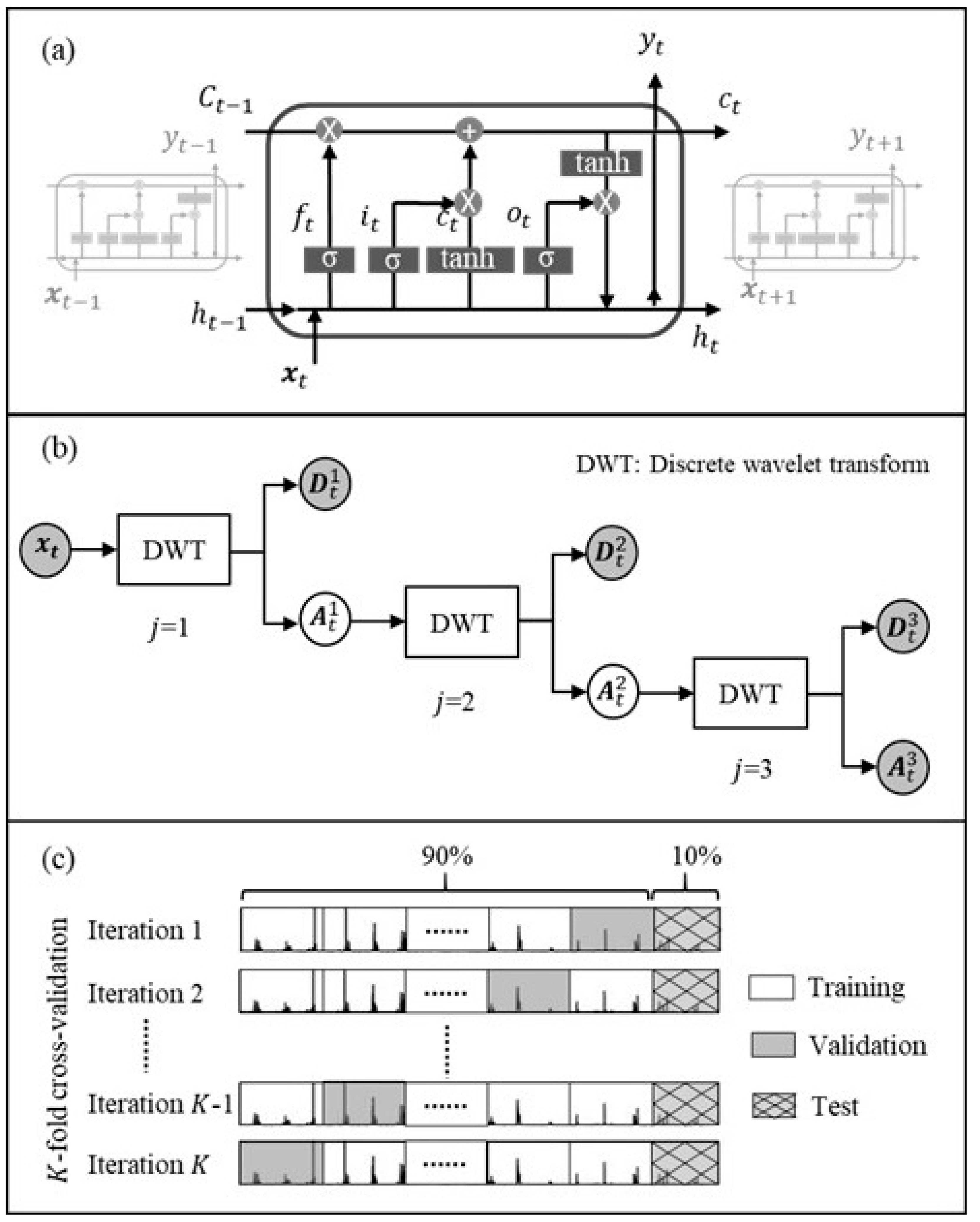
2.1. Long Short-Term Memory Network

Long short-term memory is a special kind of RNN that includes memory cells that are analogous to the states of physically based models [28]. An advantage of LSTM over an RNN is that LSTM can learn long-term dependencies between input and output features by resolving gradients that are exploding or vanishing [37]. The main difference between LSTM and RNN structures is that LSTM adds a cell state; four times more parameters should be trained because three gate functions are employed to calculate the cell and the hidden states. The internal structure of LSTM is sketched in Figure 1a.

A LSTM-based data-driven model is composed of repeating LSTM blocks, each of which contains three gates (forget gate $f_t$, input gate $i_t$, and output gate $o_t$) to determine which information is renewed, discarded, and outputted from the memory cell. Given the inputs ${\mathit{x}}_t=\left[x_{1,t},x_{2,t},\dots ,x_{N_{in},t}\right]$ at time $t$ with the number of inputs $N_{in}$, cell state $c_t$ (a long-term memory) and hidden state $h_t$ (a short-term memory) at time $t$ are computed using three gates and the cell state at a previous time step. A new state $c_t$ can be controlled through a forget gate that can forget information from the past state $c_{t-1}$ and an input gate that can accept new information from the cell update$\widetilde{c_t}$. The output gate determines how much information from the cell state $c_t$ flows into the new hidden state $h_t$. Mathematically,

$$c_t=f_t\times c_{t-1}+i_t\times \widetilde{c_t}$$

(1)

$$h_t=o_t\times \tan \mathrm{h}\left(c_t\right)$$

(2)

where the intermediate cell update $\widetilde{c_t}$ and three gates are calculated for ${\mathit{x}}_t$ and $h_{t-1}$:

$$\widetilde{c_t}=\tan \mathrm{h}\left({\mathit{W}}_{\tilde{c}}{\mathit{x}}_t+{\mathit{U}}_{\tilde{c}}{h}_{t-1}+{\mathit{b}}_{\tilde{c}}\right)$$

(3)

$$f_t=\sigma \left({\mathit{W}}_f{\mathit{x}}_t+{\mathit{U}}_f{h}_{t-1}+{\mathit{b}}_f\right)$$

(4)

$$i_t=\sigma \left({\mathit{W}}_i{\mathit{x}}_t+{\mathit{U}}_i{h}_{t-1}+{\mathit{b}}_i\right)$$

(5)

$$o_t=\sigma \left({\mathit{W}}_o{\mathit{x}}_t+{\mathit{U}}_o{h}_{t-1}+{\mathit{b}}_o\right)$$

(6)

where $\mathit{W}$, $\mathit{U}$, and $\mathit{b}$ are learnable parameters specific to the three gates and determined through the training process. The activation functions of $\sigma$ and $\tan \mathrm{h}$ are the sigmoid and the hyperbolic tangent, respectively. At $t$ = 1, the hidden and cell states are initialized as zero vectors [37]. LSTM models can also be built with more than one layer by stacking multiple layers on top of each other. The output of a stacked LSTM connects to a final “dense layer.” A target output $y_t$ can be computed from $h_t$ in the dense layer:

$$y_t={\mathit{W}}_d{h}_t+{\mathit{b}}_d$$

(7)

where ${\mathit{W}}_d$ and ${\mathit{b}}_d$ are learnable parameters known as the weight matrix and the bias term, respectively, of the dense layer. The total number of LSTM parameters is therefore 12 for each layer plus 2 for the dense layer. The shapes of these parameters can be expressed in a matrix (

Table 2. Learnable parameters of each layer of LSTM and their shapes.

Layer	Parameter	Shape
1	${\mathit{W}}_{\tilde{c}}, {\mathit{W}}_f, {\mathit{W}}_i, {\mathit{W}}_o$	[$N_{hu}$ $N_{in}$]
	${\mathit{U}}_{\tilde{c}},{\mathit{U}}_f,{\mathit{U}}_i, {\mathit{U}}_o$	[$N_{hu}$ $N_{hu}$]
	${\mathit{b}}_{\tilde{c}}, {\mathit{b}}_f, {\mathit{b}}_i, {\mathit{b}}_o$	[$N_{hu}$]
2	${\mathit{W}}_{\tilde{c}}, {\mathit{W}}_f, {\mathit{W}}_i, {\mathit{W}}_o$	[$N_{hu}$ $N_{hu}$]
	${\mathit{U}}_{\tilde{c}},{\mathit{U}}_f,{\mathit{U}}_i, {\mathit{U}}_o$	[$N_{hu}$ $N_{hu}$]
	${\mathit{b}}_{\tilde{c}}, {\mathit{b}}_f, {\mathit{b}}_i, {\mathit{b}}_o$	[$N_{hu}$ $N_{hu}$]
⋮	⋮	⋮
$N_l$	${\mathit{W}}_{\tilde{c}}, {\mathit{W}}_f, {\mathit{W}}_i, {\mathit{W}}_o$	[$N_{hu}$ $N_{hu}$]
	${\mathit{U}}_{\tilde{c}},{\mathit{U}}_f,{\mathit{U}}_i, {\mathit{U}}_o$	[$N_{hu}$ $N_{hu}$]
	${\mathit{b}}_{\tilde{c}}, {\mathit{b}}_f, {\mathit{b}}_i, {\mathit{b}}_o$	[$N_{hu}$ $N_{hu}$]
Dense	${\mathit{W}}_d$	[$N_{hu}$ $1$]
	${\mathit{b}}_d$	[$1$]

). At the beginning of training, the learnable parameters are initialized using an Xavier initialization and later optimized by the Adam algorithm, preferred in abundant studies [42].

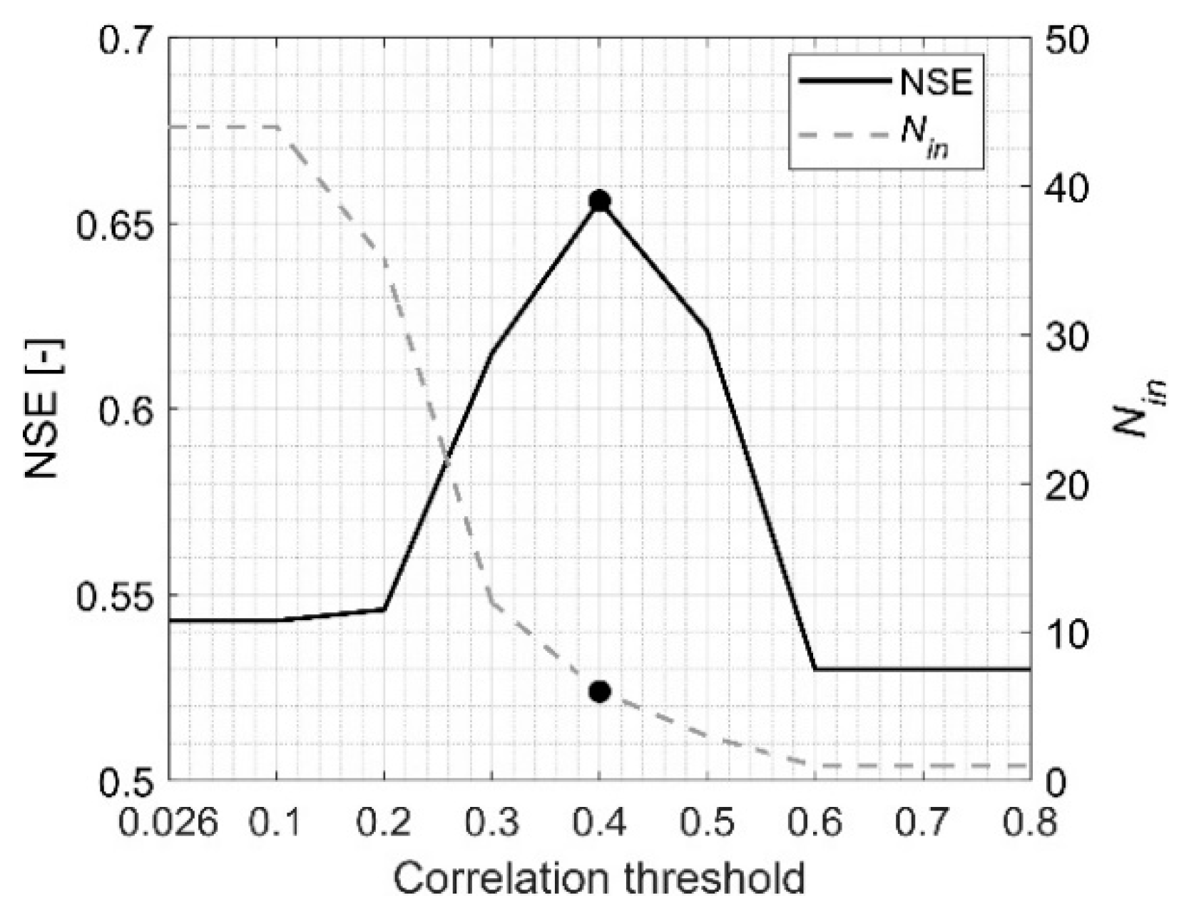
2.2. Input Predictor Selection

Maintaining a high correlation between inputs and outputs can guarantee the predictability of data-driven models. Therefore, to arrive at the optimal combination of inputs that correlate closely with the output, statistical properties of the respective time series can be used. Specifically, the cross-correlation function (CCF) and the partial autocorrelation function (PACF) are used to determine the appropriate predictors and the number of lagged values.

The CCF measures the similarity of a time series (e.g., dam inflow, $y$) with its lagged versions (e.g., candidate input variables, $\mathit{v}=\left[v_1,v_2,\dots ,v_{N_v}\right]$ with $N_v$ candidates):

$${\mathrm{CCF}}_k^{\mathit{v}y}=\frac{c_k^{\mathit{v}y}}{\sqrt{S{D}_{\mathit{v}}S{D}_y}}$$

(8)

where $k$ is the lag time; $S{D}_v$ and $S{D}_y$ are the standard deviations of$\mathit{v}$ and $y$, respectively; $c_k^{\mathit{v}y}$, which is the cross-covariance function of$\mathit{v}$ and $y$, is defined as:

$$c_k^{\mathit{v}y}=\frac{1}{N_t-1} {\displaystyle \sum }_{t=1}^{N_t-k}(y_t-\overline{y})\left({\mathit{v}}_{t+k}-\overline{\mathit{v}}\right)$$

(9)

where $t$ is the time step; $\overline{y}$ is the average of $y$; $\overline{\mathit{v}}$ is the average of $\mathit{v}$; $N_t$ denotes the number of data points of time series.

The PACF measures the linear correlation between a time series ($y_t$) and a lagged version of itself ($y_{t+k}$) and can be defined as:

$${\mathrm{PACF}}_{k,k}=\frac{{\rho }_k-{\sum }_{j=1}^{k-1}{\mathrm{PACF}}_{k-1,j}\times {\rho }_{k-j}}{1-{\sum }_{j=1}^{k-1}{\mathrm{PACF}}_{k-1,j}\times {\rho }_j}$$

(10)

where $j$ denotes an index for lag $k$; ${\rho }_k$ is an autocorrelation coefficient at lag $k$ between $y_t$ and $y_{t+k}$. At $k=1$, ${\mathrm{PACF}}_{1,1}$ is equal to ${\rho }_1$.

$${\rho }_k=\frac{{\sum }_{t=1}^{N_t-k}(y_t-\overline{y})\left(y_{t+k}-\overline{y}\right)}{{\sum }_{t=1}^{N_t}{(y_t-\overline{y})}^2}$$

(11)

Additionally, an approximate 95% confidence interval (CI) on the CCF and PACF [43] can be estimated by:

$$95\% \mathrm{CI}=-\frac{1}{N_t}\pm \frac{2}{\sqrt{N_t}}$$

(12)

Based on the calculated CCF and PACF, modelers can determine the number of antecedent values that should be included in the input vector. Other variables that may not have a significant effect on model performance can be cut off from the input vector. Generally, the CCF can be used as a reference when selecting highly correlative input predictors, while the PACF can indicate an appropriate lag for the selected variables.

2.3. Wavelet Transform

A WT is a mathematical tool that decomposes one signal into several with lower resolution levels by controlling the scaling and shifting factors of a single wavelet—the mother wavelet function exists locally as a pattern. It offers time–frequency localization of a given time series and analyzes nonstationary elements such as breakdown points, discontinuities, and local minima and maxima [35]. Due to the nature of streamflow represented by discrete signals, a discrete wavelet transform (DWT) is usually preferred in hydrological applications [33]. A DWT is easier to implement compared with a continuous wavelet transform and has a shorter computational time [44]. However, a DWT is not inherently shift-invariant. If any new values are added to the end of a time series, certain values of the wavelet component can change. This means it cannot be applied to problems related to singularity detection, forecasting, and nonparametric regression [45]. To overcome this “boundary” problem, an à trous algorithm that uses redundant information attained from observation data has been suggested [46]. The decomposition formulas of an à trous algorithm are defined as [47]:

$$D_{ t}^j= A_{ t}^{j-1}-A_{ t}^j$$

(13)

$$A_{ t}^j= {\displaystyle \sum }_{l=0}^{L-1}{g}_l{A}_{ t-2^{j-1}l mod N_t}^{j-1}$$

(14)

where $D_{ t}^j$ and $A_{ t}^j$ represent the $j$th-level wavelet (detail) and scaling (approximation) coefficients of the original time series at time $t$; $g_l$ is a scaling filter with $g_l=g_l^{\mathrm{DWT}}/\sqrt{2}$ where $g_l^{\mathrm{DWT}}$ is a scaling filter for DWT; $L$ is the length of the scaling filter; $l$ denotes an index for $L$; $mod$ refers to the modulo operator. At $j=0$, $A_{ t}^0$ is equal to the original time series of ${\mathit{x}}_t$. The latter can be obtained by the additive reconstruction:

$${\mathit{x}}_t={\displaystyle \sum }_{j=1}^{\mathrm{J}}{D}_{ t}^j+A_{ t}^{\mathrm{J}}$$

(15)

As depicted in Figure 1b, an original signal decomposes into $D_t^1$ and $A_t^1$ through the wavelet and scaling filters, and $A_t^1$ further decomposes into $D_t^2$ and $A_t^2$ through the same process. This expansion is repeated until $j$ reaches to the maximum level $\mathrm{J}$. The number of decomposed subseries is $\mathrm{J}$ + 1. For example, if $\mathrm{J}$= 3, the subseries would be [$D_t^1,D_t^2,D_t^3,A_t^3$] for each original time series. The total number of subseries for $N_{in}$ input variables is therefore $\left(\mathrm{J}+1\right)\times N_{in}$. The approximation $A^j$ becomes increasingly rough as $j$ increases. As data processing using a Daubechies 5 wavelet at level 3 has been preferred in studies of flow predictions [33,48,49,50,51], the discrete wavelet at level 3 ($\mathrm{J}$ = 3) was used in this study.

2.4. LSTM Hyper-Parameters

Configuring an LSTM network by adjusting hyper-parameters is a difficult task, but it can have a significant impact on the performance of data-driven models [37]. Additionally, the shape of the learnable parameters depends heavily on the number of inputs ($N_{in}$), the hyper-parameters of the number of hidden units ($N_{h\mathit{U}}$), and the number of layers ($N_l$), as shown in Table 2. As inappropriate values of $N_{h\mathit{U}}$ and $N_l$ can lead to unreliable LSTM models, close attention should be paid to their selection. If these values are too large, the learnable parameters that need to be trained will increase, the size of the training dataset will be large, and considerable training time will be required. Complicating matters further, too many hidden units can cause overfitting phenomena in data-driven models [52]. To compensate for this issue, a dropout technique is often used, as reducing the number of cells in the network during training can prevent overfitting. The number of cells can be adjusted from 0 to 1 depending on the dropout rate ($N_D$).

To train an LSTM network by estimating the learnable parameters $\mathit{W}$, $\mathit{U}$, and $\mathit{b}$, an objective function (or a loss function) for a given hyper-parameters must be evaluated. Here, the value of the loss function was computed from a subset (i.e., a mini-batch) of LSTM predictions and their corresponding observations; the learnable parameters during training were updated according to a given loss function at each iteration step. The number of iterations ($N_{it}$) was determined based on $N_t$, the mini-batch size ($N_{\mathit{b}}$), and the number of epochs ($N_e$) (i.e., $N_{it}$ = $N_t$/$N_{\mathit{b}}$×$N_e$). Neural networks using small batch sizes can achieve convergence with fewer epochs [53]. However, using an $N_{\mathit{b}}$ that is too small can lead to a large number of iterations, which will take excessive time to compute them. For this study, Nash–Sutcliffe efficiency (NSE) was chosen as a loss function as it can build LSTM with greater prediction accuracy compared with other metrics, such as the mean square error [54].

The hyper-parameters associated with the configuration of this study consisted of mini-batch size ($N_{\mathit{b}}$), dropout rate ($N_D$), the number of hidden units ($N_{h\mathit{U}}$), the number of layers ($N_l$), and the number of epochs ($N_e$). When tuning the hyper-parameters, two popular approaches, grid search and random search, are often used [55]. In the first approach, the grid search can be considered exhaustive as it defines a search space as a grid of hyper-parameter values and evaluates grid position for all combinations of all hyper-parameter values. A random search defines a search space as a bounded domain of hyper-parameter values and chooses random combinations in that domain for evaluations. The latter approach can create a more reliable model with more combinations of hyper-parameters, particularly when large amounts of training are used [55,56,57]. A random search was therefore used to determine an appropriate set of hyper-parameters to optimize the LSTM network in this study.

We chose a special form of resampling procedure, $K$-ld cross-validation, to evaluate the LSTM model’s performance with a limited dataset. First, the dataset was partitioned into equally (or nearly equally) $K$-sized folds or clusters. Subsequently, $K$ iterations were performed for training and validation such that within each iteration, a different fold of the dataset was held out for validation (gray cells in Figure 1c) while the remaining $K$-1 folds were used for training (white cells in Figure 1c) [58]. A useful set of hyper-parameters can provide almost equally good validation values for an object function for each iteration. To determine an appropriate number of clusters ($K$), the average of Silhouette coefficients ($\overline{s}$) is commonly used [59]. For a given data point $i$ in a cluster, the Silhouette coefficient $s\left(i\right)$ is defined as:

$$s\left(i\right)=\frac{b\left(i\right)-a\left(i\right)}{max\left\{a\left(i\right),b\left(i\right)\right\}}$$

(16)

where $a\left(i\right)$ is the average distance between point $i$ and all other points in the same cluster, and $b\left(i\right)$ is the average distance between the point $i$ and all points in the nearest cluster. It is advisable to choose a $K$ that provides a high value of $\overline{s}$.

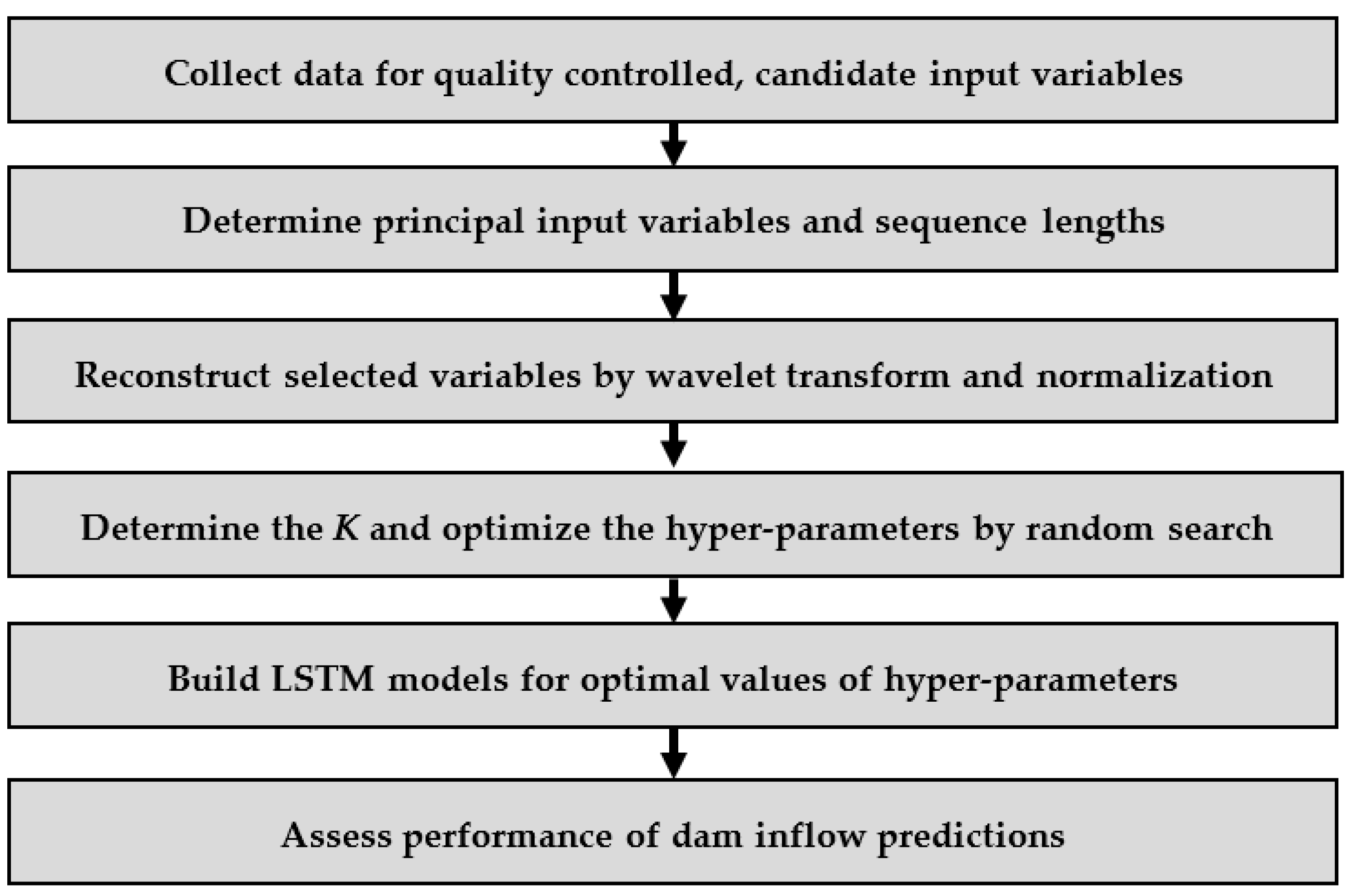
2.5. Summary of Modeling Framework

A brief overview of the methodology adopted for dam inflow prediction, hereafter called SWLSTM, follows the schematic in Figure 2:

(1)

Collect the time series of both the target output $y_t$ (i.e., dam inflow) and the candidate input predictors ${\mathit{v}}_t=\left[v_{1,t},v_{2,t},\dots ,v_{N_v,t}\right]$, $t=1,\dots ,N_t$. Any inappropriate or missing values in the collected data should be reviewed carefully.

(2)

Determine the explanatory “principal” variables ${\mathit{x}}_t=\left[x_{1,t},x_{2,t},\dots ,x_{N_{in},t}\right]$, $t=1,\dots ,N_t$ among the candidate predictors, with an appropriate lag time, using the CCF and PACF.

(3)

Decompose and reconstruct the selected input predictors into the wavelet-transformed subseries$\left[D_{1,t}^1,D_{1,t}^2,D_{1,t}^3,A_{1,t}^3,\dots ,D_{N_{in},t}^1,D_{N_{in},t}^2,D_{N_{in},t}^3,A_{N_{in},t}^3\right]$. These reconstructed data are normalized to values between 0 and 1, and then split into one set for training and validation and another for testing. In this study, we set 90% of the total data length for training and validation and 10% for test.

(4)

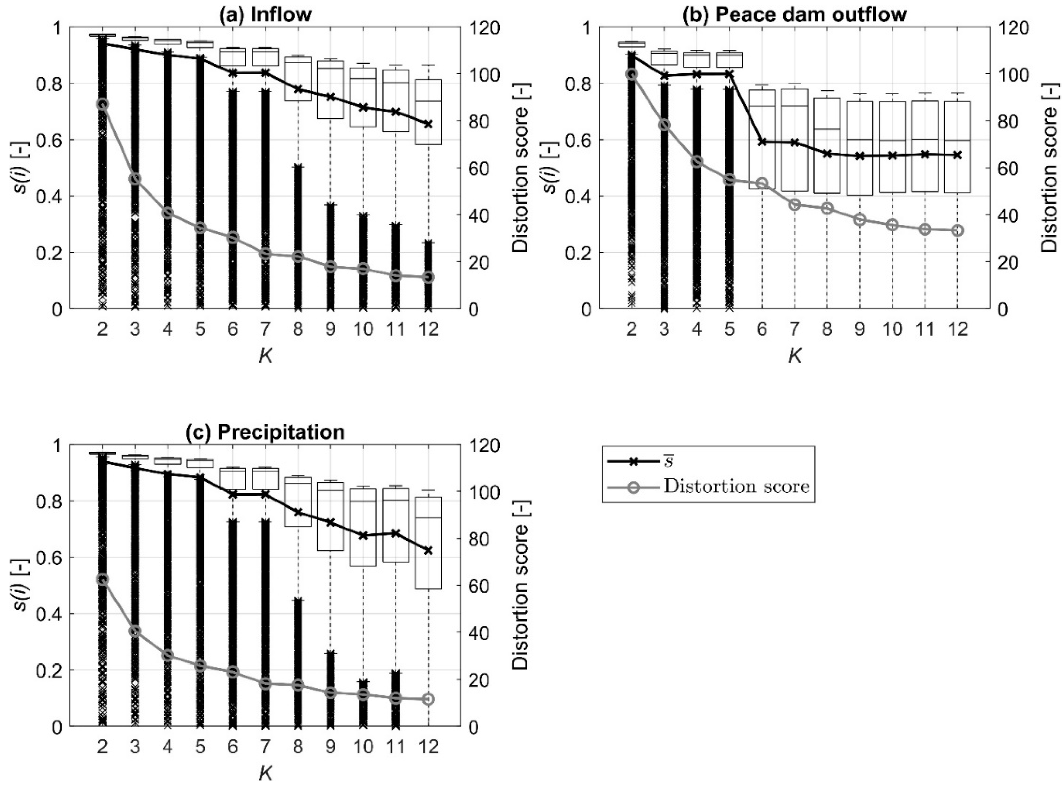
Determine the number of clusters for the $K$-fold cross-validation and then optimize five hyper-parameters by the random search over the training and validation set.

(5)

Train and build the LSTM models, using the optimal values of hyper-parameters over the training and validation set.

(6)

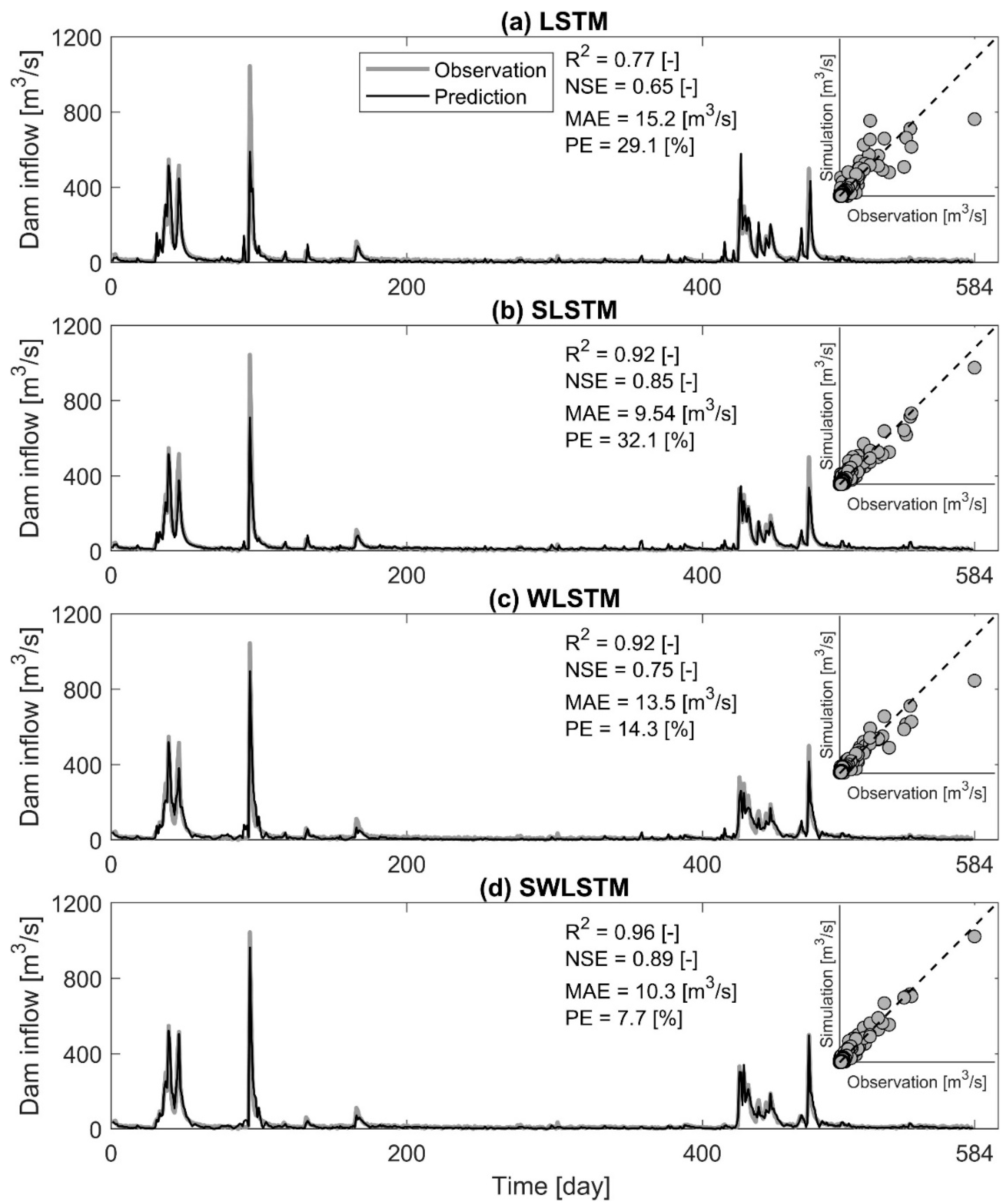
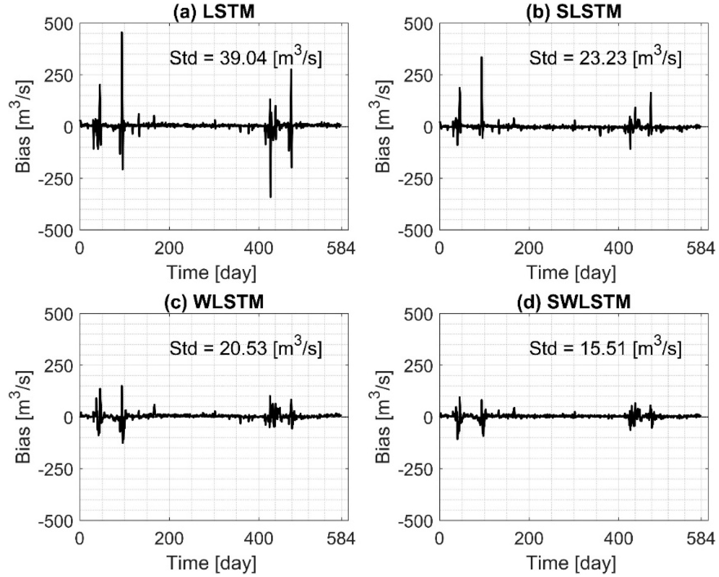
Assess and compare the performance of LSTM models in predicting dam inflow for the test dataset. The LSTM models chosen to demonstrate the effectiveness of SWLSTM presented here are (1) a regular LSTM without both the determination of principal lags and variables and the WT, (2) a “WLSTM,” which is a regular LSTM coupled with a WT, and (3) a “SLSTM,” which is similar to a regular LSTM but performs the input specification in the Step 2.

2.6. Evaluation Metrics

Three evaluation metrics of NSE, mean absolute error (MAE), and peak error (PE) were used to qualitatively measure the performance of model accuracy. Each was computed over the test period as:

$$\mathrm{NSE}=1-\frac{{\sum }_{t=1}^{N_t}{\left(y_t-y_t^{o\mathit{b}s}\right)}^2}{{\sum }_{t=1}^{N_t}{\left(y_t^{o\mathit{b}s}-\overline{y^{o\mathit{b}s}}\right)}^2}$$

(17)

$$\mathrm{MAE}= \frac{{\sum }_{t=1}^{N_t}\left|y_t-y_t^{o\mathit{b}s}\right|}{N_t}$$

(18)

$$\mathrm{PE}= \frac{\left|y_{max}^{o\mathit{b}s}-y_{max}\right|}{y_{max}^{o\mathit{b}s}}\times 100$$

(19)

where $y_t^{o\mathit{b}s}$ denotes the observation of dam inflow at time $t$; $\overline{y^{o\mathit{b}s}}$ is the average of $y^{o\mathit{b}s}$; $y_{max}$ and $y_{max}^{o\mathit{b}s}$ are the predicted and observed peak dam inflow, respectively.

2.7. Open Source Software

Our research relies on open source software with the programing language of Python 3.7 [60]. The libraries of Numpy [61], Pandas [62] and Scikit-learn [63] were used for managing and preprocessing the data. TensorFlow [64] and Keras [65] were utilized to implement LSTM. The hardware environment was configured with Intel(R) Xeon(R) Gold 6242 CPU at 2.80 GHz × 32 processors, and 376 GB of RAM.

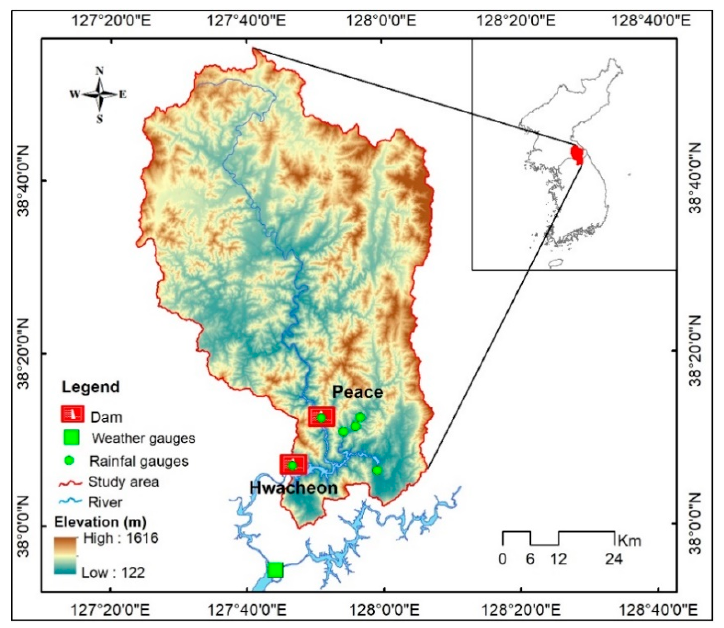
3. Study Area and Dataset

The Hwacheon dam watershed in the central part of the Korean Peninsula (its latitude and longitude are 127°47′ E and 38°7′ N, respectively) was chosen as a case study (Figure 3). The watershed created by the dam covers 3901 km², approximately 80% of which is forest, and its elevation varies from close to 120 m at the dam site to 1600 m. The Hwacheon dam was designed as a multipurpose dam for generate electricity, prevent floods, and store water. Its power generation capacity is 326 GWh and its total storage capacity is approximately 1018 Mm³, making it a relatively large dam for South Korea. The Peace dam, located upstream of the Hwacheon dam, was built to prevent flooding and prepare for North Korean military (flood) attacks, and is normally operated as a dry-water dam. A daily dataset for 5844 days from 1 January 2004, to 31 December 2019 was collected and is described in

Table 3. Information about the data used for predicting the inflow of the Hwacheon dam.

Variable *	Station Name	Station ID	Longitude	Latitude	Source
Qin (m3/s)	Hwacheon dam	1010310	127°46′60″	38° 7′0″	Water Resources Management Information System (http://www.wamis.go.kr:8081/ENG/, accessed on 1st January 2020)
Qo (m3/s)	Peace dam	1009710	127°50′55″	38°12′43″
Pr (mm)	Hwacheongunchung	10094010	127°50′54″	38°12′34″
	Bangsanchogyo	10104030	127°56′35″	38°12′36″
	Hwacheondam	10104050	127°46′38″	38° 7′2″
	Geumakri	10104060	127°55′52″	38°11′36″
	Suibcheon	10104170	127°54′5″	38°10′59″
	Yanggu Seocheon	10104171	127°59′3″	38° 6′28″
Ta (°C)	Chuncheon	101	127°44′8.51″	37°54’59.27″	Automated Surface Observing System (https://data.kma.go.kr/cmmn/main.do, accessed on 1st January 2020)
H (%)
Ws (m/s)
Pre (hPa)

* Qin: inflow to Hwacheon dam; Qo: outflow from Peace dam; Pr: precipitation; Ta: temperature; H: humidity; Ws: wind speed; Pre: pressure.

. Wherein, the first 5260 days (90% of the total data) were used for training and validation, while the rest was left for testing the trained models. The data collected includes inflow to the Hwacheon dam (Qin), dam outflow from Peace dam (Qo), and meteorological data such as precipitation (Pr), temperature (Ta), humidity (H), wind speed (Ws), and pressure (Pre). Any inappropriate (negative) or missing values in the collected data were replaced with those interpolated linearly. The amount of such an inappropriate data is however less than 0.01%. Spatially averaged precipitation was computed using Thiessen polygons for six rain gauges in Table 3 and Figure 3.

4. Results and Discussion

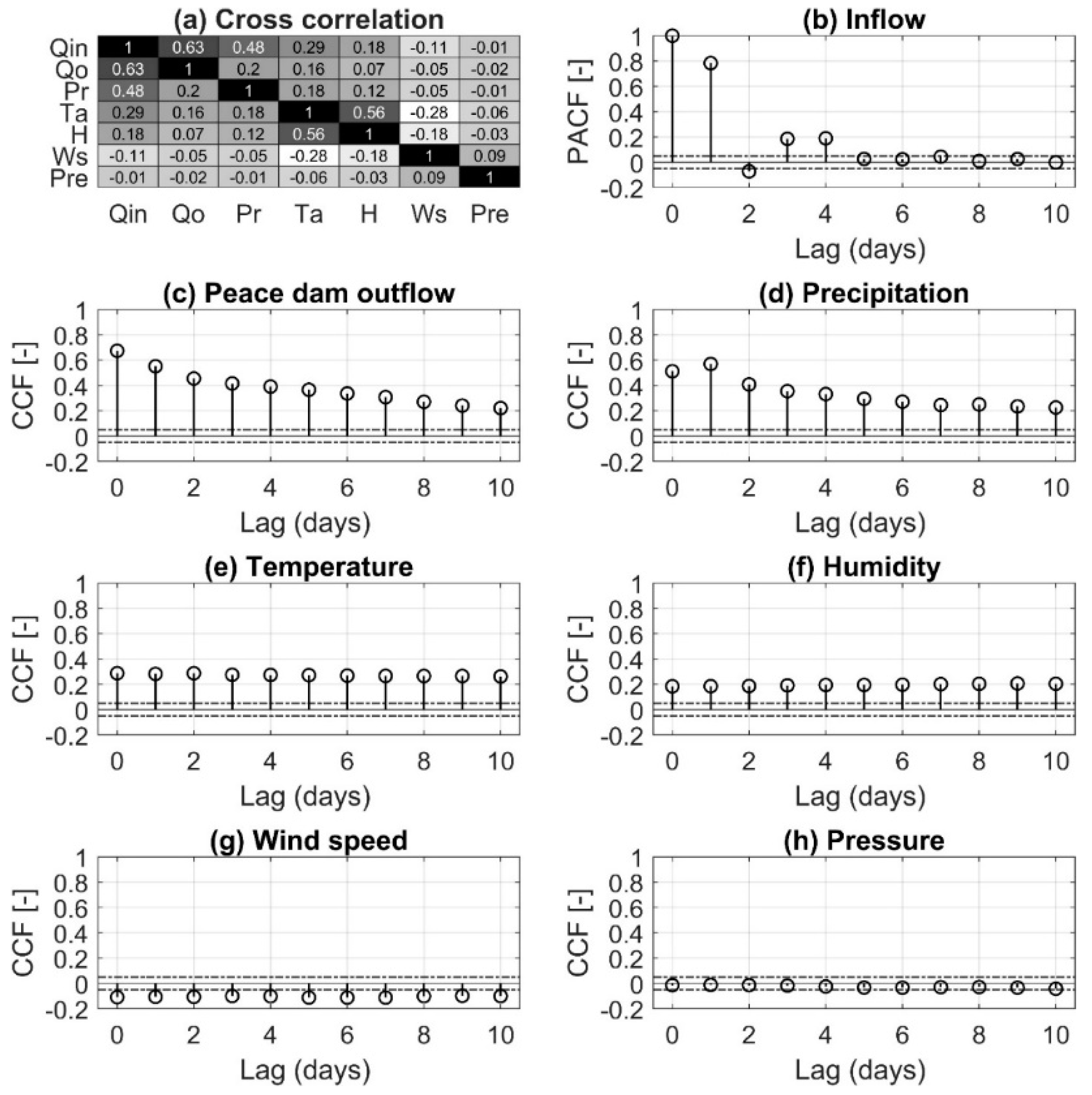
4.1. Determining Principal Input Predictors and Their Sequence Lengths

To construct an appropriate input combination for the LSTM model, the principal variables and sequence lengths were determined using the statistical properties of the candidate variables. Figure 4 provides the statistical correlations between the seven candidate input variables (i.e., Qin, Qo, Pr, Ta, H, Ws, and Pre) and the target variable (Qin). Figure 4a shows the CCF between the seven candidate variables with a time lag of zero, indicating that Qo and Pr were strongly correlated with Qin (their CCFs were approximately 0.63 and 0.48, respectively); Ta and H had a relatively weaker correlation with Qin; and Ws and Pre had a negative correlation with Qin. The correlations for other combinations of the remaining variables were all less than 0.2, with the exception of the correlation between H and Ta. Regarding the correlations between Qin and the seven candidate variables at different time lags from 0 to 10, Figure 4b shows that Qin had a strong autocorrelation up to a 1-day lag (the PACF is approximately 0.8), and the correlation became significantly lower when the time lag was greater than 1 day. The CCF values for Qo and Pr, which had a strong correlation with Qin, became smaller as the time lag increased, while the values for the remaining four variables were not influenced by the magnitude of the time delay (see Figure 4c–h).

Based on the PACF and CCF analyses, a final set of input variables and sequence lengths (time lags) that had a high correlation with the target output Qin were selected. However, choosing only the input variables and the lags that have a close correlation with the target variable posed some challenges. In previous research, such a selection was typically based on user decisions made through trial and error, and no specific rules or criteria were used to determine the which key inputs were optimal [5,37,66]. We proposed a robust analysis using a “correlation threshold” for the PCAF and CCF values, and only variables greater than this threshold were used as input predictors and their time lags to construct and train a model. If the correlation threshold was small (e.g., 0.026, the upper bound of the 95% CI from Equation (12)), most of the variables and sequence lengths could be adopted to predict the target variable. Conversely, if the threshold was large (e.g., 0.8), the SLSTM model was constructed using only a limited number of predictors that were highly correlated with the target variable. Figure 5 depicts the performance of the SLSTM against the correlation threshold as a loss function (NSE). A model trained on a threshold of 0.4 produced the highest NSE value of 0.66, which was considered optimal. The model performed the poorest with a small threshold of 0.026, which means that a large number of inputs (up to 44 in this study) that were not highly correlated with the target variable led to overfitting and less-accurate outcomes. However, if using a high threshold (greater than 0.6), the number of input predictors may be limited (only 1 in this study) and not be sufficient to describe the target variable. By selecting the principal variables and their corresponding sequence lengths based on the optimal threshold of 0.4, ${\mathrm{Qin}}_{t-1}$, ${\mathrm{Qo}}_{t-1}$, ${\mathrm{Qo}}_{t-2}$, ${\mathrm{Qo}}_{t-3}$, ${\mathrm{Pr}}_{t-1}$, and ${\mathrm{Pr}}_{t-2}$ became the inputs to predict the inflow of Hwacheon dam.

4.2. Decomposing Input Time Series by a Wavelet Transform

Three levels of DWT decomposition were performed on the seven candidate input variables for WLSTM and the six selected inputs defined above for SWLSTM, extracting four subseries for each. Figure 6 shows the original and transformed time series of the three principal variables of Qin, Qo, and Pr. The degree of fluctuations in the “Detail” time series is smoother and has a lower frequency at higher decomposition levels. The “Approximation” $A^3$ has a rougher and slower gradual trend than the original time series $\mathit{x}$.

Data processing by the three levels of decomposition created an additional time series that is five times the number of the original time series (i.e., one original time series plus four decomposed time series). Eventually, the inputs used to train the LSTM models presented in this study and predict dam inflow were (1) for LSTM, all seven candidate variables at t-1 timestep (i.e., ${\mathrm{Qin}}_{t-1}$, ${\mathrm{Qo}}_{t-1}$, ${\mathrm{Pr}}_{t-1}$, ${\mathrm{Ta}}_{t-1}$, ${\mathrm{H}}_{t-1}$, ${\mathrm{Ws}}_{t-1}$, and ${\mathrm{Pre}}_{t-1}$); (2) for SLSTM, six variables selected from the above “correlation threshold” analysis (i.e., ${\mathrm{Qin}}_{t-1}$, ${\mathrm{Qo}}_{t-1}$, ${\mathrm{Qo}}_{t-2}$, ${\mathrm{Qo}}_{t-3}$, ${\mathrm{Pr}}_{t-1}$, and ${\mathrm{Pr}}_{t-2}$); (3) for WLSTM, in addition to the seven candidate variables, subtime series on each by WT (for a total of 35 inputs); (4) for SWLSTM, a total of 30 variables made by WT on the six variables. For more details, see

Table 4. Summary of input and output variables used for training four data-driven models (LSTM, SLSTM, WSLTM, and SWLSTM).

Model	x	y
LSTM	${\mathrm{Qin}}_{t-1},{ \mathrm{Qo}}_{t-1},{ \mathrm{Pr}}_{t-1},{ \mathrm{Ta}}_{t-1},{\mathrm{H}}_{t-1},{\mathrm{Ws}}_{t-1},{\mathrm{Pre}}_{t-1}$	${\mathrm{Qin}}_{\mathrm{t}}$
SLSTM	${\mathrm{Qin}}_{t-1},{\mathrm{Qo}}_{t-1},{\mathrm{Qo}}_{t-2},{\mathrm{Qo}}_{t-3},{\mathrm{Pr}}_{t-1},{\mathrm{Pr}}_{t-2}$
WLSTM	$\begin{array}{l}{\mathrm{Qin}}_{t-1},D_{\mathrm{Qin}, t-1}^1,D_{\mathrm{Qin}, t-1}^2,D_{\mathrm{Qin}, t-1}^3, A_{\mathrm{Qin}, t-1}^3,\\ {\mathrm{Qo}}_{t-1},D_{\mathrm{Qo}, t-1}^1,D_{\mathrm{Qo}, t-1}^2,D_{\mathrm{Qo}, t-1}^3, A_{\mathrm{Qo}, t-1}^3,\\ {\mathrm{Pr}}_{t-1},D_{\mathrm{Pr}, t-1}^1,D_{P\mathrm{r}, t-1}^2,D_{\mathrm{Pr}, t-1}^3, A_{\mathrm{Pr},t-1}^3,\\ {\mathrm{Ta}}_{t-1},D_{\mathrm{Ta}, t-1}^1,D_{\mathrm{Ta},t-1}^2,D_{\mathrm{Ta},t-1}^3, A_{\mathrm{Ta},t-1}^3,\\ {\mathrm{H}}_{t-1},D_{\mathrm{H},t-1}^1,D_{\mathrm{H},t-1}^2,D_{\mathrm{H}, t-1}^3, A_{\mathrm{H},t-1}^3,\\ {\mathrm{Ws}}_{t-1},D_{\mathrm{Ws},t-1}^1,D_{\mathrm{Ws},t-1}^2,D_{\mathrm{Ws},t-1}^3, A_{\mathrm{Ws},t-1}^3,\\ {\mathrm{Pre}}_{t-1},D_{\mathrm{Pre},t-1}^1,D_{\mathrm{Pre},t-1}^2,D_{\mathrm{Pre},t-1}^3, A_{\mathrm{Pre},t-1}^3\end{array}$
SWLSTM	$\begin{array}{l}{\mathrm{Qin}}_{t-1},D_{\mathrm{Qin}, t-1}^1,D_{\mathrm{Qin}, t-1}^2,D_{\mathrm{Qin}, t-1}^3, A_{\mathrm{Qin}, t-1}^3, \\ {\mathrm{Qo}}_{t-1},D_{\mathrm{Qo}, t-1}^1,D_{\mathrm{Qo}, t-1}^2,D_{\mathrm{Qo}, t-1}^3, A_{\mathrm{Qo}, t-1}^3,\\ {\mathrm{Qo}}_{t-2},D_{\mathrm{Qo}, t-2}^1,D_{\mathrm{Qo}, t-2}^2,D_{\mathrm{Qo}, t-2}^3, A_{\mathrm{Qo}, t-2}^3,\\ {\mathrm{Qo}}_{t-3},D_{\mathrm{Qo}, t-3}^1,D_{\mathrm{Qo}, t-3}^2,D_{\mathrm{Qo}, t-3}^3, A_{\mathrm{Qo}, t-3}^3,\\ {\mathrm{Pr}}_{t-1},D_{\mathrm{Pr}, t-1}^1,D_{\mathrm{Pr}, t-1}^2,D_{\mathrm{Pr}, t-1}^3, A_{\mathrm{Pr},t-1}^3,\\ {\mathrm{Pr}}_{t-2},D_{\mathrm{Pr}, t-2}^1,D_{\mathrm{Pr}, t-2}^2,D_{\mathrm{Pr}, t-2}^3, A_{\mathrm{Pr},t-2}^3\end{array}$

.

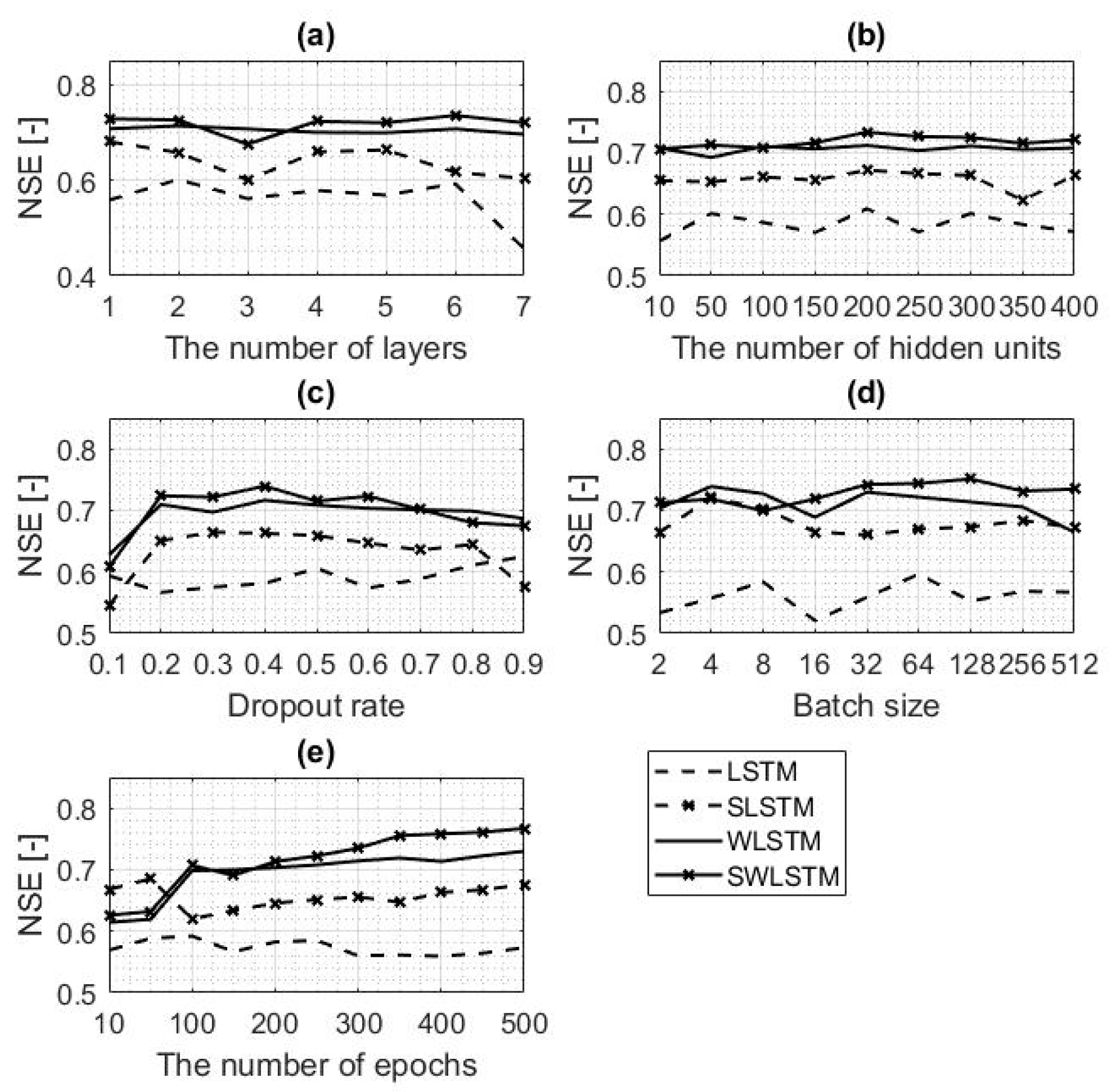
4.3. Optimizing the Hyper-Parameters

Choosing an appropriate set of hyper-parameters significantly affected model performance. To investigate the effects of the five hyper-parameters on the value of the loss function (i.e., NSE), their configurations were set as listed in

Table 5. The configurations of the hyper-parameters to investigate the effects of each hyper-parameter on the model performance in Figure 7. The controlled value for each hyper-parameter was borrowed from Kratzert, Klotz [37].

	The Number of Layers	The Number of Hidden Units	Dropout Rate	Batch Size	The Number of Epochs
Figure 7a	1, 2, 3, 4, 5, 6, 7	100	0.1	512	200
Figure 7b	1	10, 50, 100, 150, 200, 250, 300, 350, 400	0.1	512	200
Figure 7c	1	20	0.1, 0.2, 0.3, 0.4, 0.5, 0.6, 0.7, 0.8, 0.9	512	200
Figure 7d	1	20	0.1	2, 4, 8, 16, 32, 64, 128, 256, 512	200
Figure 7e	1	20	0.1	512	10, 50, 100, 200, 250, 300, 350, 400, 450, 500

, with controlled values suggested by Kratzert, Klotz [37]. As shown in Figure 7, change in NSE values was negligible (neither increasing nor decreasing) as the value of each hyper-parameter increased. SWLSTM consistently provided the largest NSE, with values in the range of 0.7–0.8, while LSTM provided the smallest NSE range of 0.5–0.6. These results indicate in part that SWLSTM outperformed the other models.

In this study, an optimal hyper-parameter set for the four data-driven models was determined from $K$-fold cross-validation and the random search. First, an appropriate number of clusters for $K$-fold cross-validation was chosen based on the average Silhouette coefficients, $\overline{s}$, and the “distortion score” of the elbow method (Figure 8). In general, $K$ values can be selected that provide a high value of $\overline{s}$ and those corresponding to the “elbow” of the distortion score curve. As $K$ increased, the $\overline{s}$ value tended to decrease overall, so $K$ values from 2 to 5 could be chosen. The gray dashed line in Figure 8 shows an elbow with a $K$ near 5–7. A $K$ of 5 was therefore selected to optimize the hyper-parameters of the four data-driven models in this study.

For a $K$ of 5 and a confined range specified in the second column of

Table 6. The prior ranges of the hyper-parameters used in the Random search (see the second column) and determined optimal values of the hyper-parameters for four data-driven models by random search and $K$-fold cross-validation with $K$ of 5 (see the rest columns).

Hyper-Parameters	Range	LSTM	SLSTM	WLSTM	SWLSTM
The number of layers	[1–7]	2	2	2	2
The number of hidden units	[10–400]	100	150	200	200
The number of epochs	[10–500]	250	250	250	250
Dropout rate	[0.1–0.9]	0.3	0.5	0.5	0.6
Batch size	[2–512]	8	8	32	32

, a set of hyper-parameters for the four models was found using the random search method (see Table 6 for the optimal hyper-parameter set). As a result, two LSTM layers were required for all four models, while the values of other hyper-parameters varied. Specifically, WLSTM and SWLSTM required a larger number of hidden units, epochs, dropout, and batch size compared with the other two models. Such a complex configuration was required because the amount of inputs used by WLSTM and SWLSTM was five times more than in other models. The CPU time required for this process is 2–6 min, much more than LSTM training that takes about 50 s and other processes (LSTM prediction, wavelet transformation, and normalization) that only take a few seconds.

4.4. Predicting Dam Inflow with Trained LSTMs

LSTM models trained using optimal hyper-parameters were applied to the test dataset to predict inflow at the Hwacheon dam. Comparing the hydrographs with observations, the overall variation and magnitude of predicted inflow using SWLSTM agreed more closely with observations than did the results produced by other models (Figure 9). Quantitatively, SWLSTM had an R² of 0.96 in a 1:1 comparison between prediction and observation, which outperformed the 0.77, 0.92, and 0.92 values produced by LSTM, SLSTM, and WLSTM, respectively. The results produced by NSE, MAE, and PE confirm that the predictions from SWLSTM were closest to observations. In particular, compared with LSTM, which has an NSE of 0.65 and a PE of 29.1%, both metrics were significantly improved to an NSE of 0.89 and a PE of 7.7% (see Figure 9 for specific values).

To examine the superiority of SWLSTM proposed in this study compared with the other models, a relative “difference” metric (Δ) in Equation (20) was introduced:

$$∆=\frac{\left|{Metric}_A-{Metric}_{ideal}\right|-\left|{Metric}_B-{Metric}_{ideal}\right|}{\left|{Metric}_A-{Metric}_{ideal}\right|}\times 100$$

(20)

where $Metri{c}_A$ and $Metri{c}_{\mathit{B}}$ are the values of a metric for two models A and B, $Metri{c}_{ideal}$ represents the ideal (perfect) value of the metrics of R², NSE, MAE, and PE (1, 1, 0, and 0, respectively). The positive (or negative) values of ∆ indicate that the prediction results of model B are more (or less) accurate than those computed by model A.

Table 7. Accuracy improvements of SWLSTM to three other models of LSTM, SLSTM, and WLSTM for dam inflow predictions for the test dataset. A relative “difference” metric (${∆}_{Metric}$) in Equation (20) is computed for four evaluation metrics (R2, NSE, MAE, and PE). The positive (or negative) values of ${∆}_{Metric}$ indicate that the prediction results of SWLSTM are more (or less) accurate than those computed by other models. The optimal hyper-parameters specified in Table 6 and the 5-folds (K = 5) are employed.

Relative “Difference” Metric (%)	SWLSTM vs. LSTM	SWLSTM vs. SLSTM	SWLSTM vs. WLSTM
${∆}_{{\mathrm{R}}^2}$	82.5	50	49.5
${∆}_{\mathrm{NSE}}$	68.4	27.7	53.4
${∆}_{\mathrm{MAE}}$	29.8	−8.4	25.5
${∆}_{\mathrm{PE}}$	75	77.3	48.8

shows that the accuracy performance of SWLSTM was superior to that of LSTM, SLSTM, and WLSTM.

Based on these results, we concluded that the selection of appropriate input predictors and time lags helped create a more reliable data-driven model (see comparisons of SLSTM vs. LSTM and SWLSTM vs. WLSTM). In general, all factors related to weather and hydrology as well as the past histories of each variable, can affect dam inflow predictions, but using too much information that is not highly correlated (Figure 4) creates an overfitting model. As the number of input data increases, the noise for that input will also increase, and it is difficult to accurately estimate weights (or learnable parameters) for each input. Additionally, the historical period that affects the future inflow varies depending on the predictor. For example, Qin is closely related to itself a day ago, while for Qo and Pr, data from 3 and 2 days ago are also important.

It is interesting to note that the use of WT improved the flood peak predictability of data-driven models. That is, the PE values of WLSTM and SWLSTM were approximately one-half and one-quarter the size of those from LSTM and SLSTM, respectively. Additionally, near the flood peak in the test dataset, the bias values for both models using WT were much smaller than those for the non-WT models (Figure 10). With the aid of WT, five times as much data were used, and they can be reconstructed with various levels of decomposition. To train extreme data such as flood peaks, including separate time series such as WT appeared to be effective. If only one original data point was used for training, abnormally extreme high-frequency data may be considered noisy rather than critical information to be learned, which may fail to recognize, learn, and predict these events.

4.5. Feasibility to Multimodal, Multitask, and Bidirectional Learning

Recently, multimodal, multitask, and bidirectional learning has received great interest [33,34,66,67], and it is worth discussing the feasibility of hydrological time series predictions (e.g., dam inflow, runoff, or flood predictions). First, both multimodal learning with multiple inputs and multitask learning with multiple outputs are related to high-dimensional problems. In hydrological time series predictions, there are three reasons for increasing the dimension, namely, a case where the number of input or output variables is large, a case where the sequence length or lead time of each variable is long, and a case where the values of the variables vary spatially. In the latter case, the number of dimensions can increase significantly up to O(10² to 10⁶) while it is not very large, O(10⁰ to 10¹) in the first two cases. In this study, multimodal learning for the first two cases was performed with a maximum of 30 dimensions. As a future study, it will be necessary to review the learning ability for ultra-high-dimensional problems that can take into account the spatial heterogeneity of variables.

The second is to examine the applicability of bidirectional learning in predicting hydrologic time series. Several studies have mentioned the superiority of bidirectional learning [68], which combines information from both the past and the future at the same time. However, this is limited to predictions of language models or hindcasting problems in which future data exist. It is challenging to apply it to hydrological forecasting cases because future information about weather variables (e.g., precipitation) and human (e.g., dam) operation is unknown at the present time.

5. Conclusions

In this study, data-driven models based on an LSTM network were built to predict daily inflow at the Hwacheon dam in South Korea. Three important aspects were considered to improve the accuracy of dam inflow predictions in an integrated fashion: (1) principal input predictors and their time lags were determined from a robust analysis of the statistical properties of the data series; (2) the original time series was converted to multiscale subseries by a WT; (3) hyper-parameters of all models were efficiently optimized through $K$-fold cross-validation and the random search. The effectiveness of SWLSTM, a model trained to consider these aspects, was compared with LSTM (trained without input selection and data transformation), SLSTM (trained with input selection only), and WLSTM (trained with data transformation only). The primary findings of this study are presented in the following paragraphs.

First, seven candidate input variables (i.e., inflow to the Hwacheon dam, outflow from Peace dam, precipitation, temperature, humidity, wind speed, and pressure) were initially chosen to investigate the correlation properties for the target output, Qin. Based on PACF and CCF analyses, we selected a final set of input variables and their sequence lengths (time lags). However, how to choose only the input variables and the lags that are closely correlated with the target variable remains an open question. In this study, a robust analysis using a correlation threshold for the PCAF and CCF values was proposed, and only variables greater than this threshold were selected as input predictors and their time lags. As shown in Figure 5, a model trained on a threshold of 0.4 produced the highest NSE value. Eliminating variables that have a low correlation with Qin helped prevent divergence and restrict overfitting in the learning model. Conclusively, ${\mathrm{Qin}}_{t-1}$, ${\mathrm{Qo}}_{t-1}$, ${\mathrm{Qo}}_{t-2}$, ${\mathrm{Qo}}_{t-3}$, ${\mathrm{Pr}}_{t-1}$, and ${\mathrm{Pr}}_{t-2}$ become the principal inputs to predict the inflow of the dam. The effectiveness of such an input specification was validated because the models using it (SLSTM and SWLSTM) provided exceptionally accurate predictions compared with the unused models (i.e., LSTM and WLSTM).

Second, using additional data series reconstructed by a WT improved predictability, particularly for flow peak (see the comparisons of WLSTM vs. LSTM and SWLSTM vs. SLSTM). The PE values of WLSTM and SWLSTM were approximately one-half and one-quarter the size of those produced by LSTM and SLSTM, respectively. For training extreme data such as flow peaks, including separate time series by WT can be effective. If only one original data point is used for training, abnormally extreme high-frequency data may be considered noisy rather than critical information to be learned, and the system may fail to recognize, learn, and predict these events.

Third, for a $K$ of 5 as determined by the Silhouette coefficients and the distortion score (Figure 8), a set of hyper-parameters for the four models was found using a random search (Table 6). Both WLSTM and SWLSTM require a larger number of hidden units, epochs, dropout, and batch size compared with the other two models. The need for this complex configuration is clear because the amount of inputs used by WLSTM and SWLSTM was five times greater than that of the other models.

Last, accuracy performance investigated by various evaluation metrics revealed that SWLSTM is superior to LSTM, SLSTM, and WLSTM by 84%, 78%, and 65%, respectively. When the SWLSTM framework in this study is coupled with the procedures of a WT and the input specifications, overall and peak accuracy of time-dependent flow prediction improved. Ultimately, accurate forecasts of inflow will help policy makers and operators better manage their reservoir operations and tasks.

References

1. Jothiprakash, V.; Magar, R.B. Multi-time-step ahead daily and hourly intermittent reservoir inflow prediction by artificial intelligent techniques using lumped and distributed data. J. Hydrol. 2012, 450–451, 293–307. [Google Scholar] [CrossRef]
2. El-Shafie, A.; Taha, M.R.; Noureldin, A. A neuro-fuzzy model for inflow forecasting of the Nile river at Aswan high dam. Water Resour. Manag. 2006, 21, 533–556. [Google Scholar] [CrossRef]
3. Seo, Y.; Kim, S.; Kisi, O.; Singh, V.P. Daily water level forecasting using wavelet decomposition and artificial intelligence techniques. J. Hydrol. 2015, 520, 224–243. [Google Scholar] [CrossRef]
4. Yang, T.; Asanjan, A.A.; Welles, E.; Gao, X.; Sorooshian, S.; Liu, X. Developing reservoir monthly inflow forecasts using artificial intelligence and climate phenomenon information. Water Resour. Res. 2017, 53, 2786–2812. [Google Scholar] [CrossRef]
5. Zemzami, M.; Benaabidate, L. Improvement of artificial neural networks to predict daily streamflow in a semi-arid area. Hydrol. Sci. J. 2016. [Google Scholar] [CrossRef] [Green Version]
6. He, Z.H.; Tian, F.Q.; Gupta, H.V.; Hu, H.C.; Hu, H.P. Diagnostic calibration of a hydrological model in a mountain area by hydrograph partitioning. Hydrol. Earth Syst. Sci. 2015, 19, 1807–1826. [Google Scholar] [CrossRef] [Green Version]
7. Chen, Y.; Zhou, H.; Zhang, H.; Du, G.; Zhou, J. Urban flood risk warning under rapid urbanization. Env. Res 2015, 139, 3–10. [Google Scholar] [CrossRef] [PubMed]
8. Fatichi, S.; Vivoni, E.R.; Ogden, F.L.; Ivanov, V.Y.; Mirus, B.; Gochis, D.; Downer, C.W.; Camporese, M.; Davison, J.H.; Ebel, B.; et al. An overview of current applications, challenges, and future trends in distributed process-based models in hydrology. J. Hydrol. 2016, 537, 45–60. [Google Scholar] [CrossRef] [Green Version]
9. Kim, J.; Ivanov, V.Y. On the nonuniqueness of sediment yield at the catchment scale: The effects of soil antecedent conditions and surface shield. Water Resour. Res. 2014, 50, 1025–1045. [Google Scholar] [CrossRef]
10. Kim, J.; Ivanov, V.Y.; Katopodes, N.D. Hydraulic resistance to overland flow on surfaces with partially submerged vegetation. Water Resour. Res. 2012, 48. [Google Scholar] [CrossRef] [Green Version]
11. Kim, J.; Dwelle, M.C.; Kampf, S.K.; Fatichi, S.; Ivanov, V.Y. On the non-uniqueness of the hydro-geomorphic responses in a zero-order catchment with respect to soil moisture. Adv. Water Resour. 2016, 92, 73–89. [Google Scholar] [CrossRef] [Green Version]
12. Warnock, A.; Kim, J.; Ivanov, V.; Katopodes, N.D. Self-Adaptive Kinematic-Dynamic Model for Overland Flow. J. Hydraul. Eng. 2014, 140, 169–181. [Google Scholar] [CrossRef]
13. Tran, V.N.; Dwelle, M.C.; Sargsyan, K.; Ivanov, V.Y.; Kim, J. A Novel Modeling Framework for Computationally Efficient and Accurate Real-Time Ensemble Flood Forecasting With Uncertainty Quantification. Water Resour. Res. 2020, 56. [Google Scholar] [CrossRef]
14. Tran, V.N.; Kim, J. Quantification of predictive uncertainty with a metamodel: Toward more efficient hydrologic simulations. Stoch. Environ. Res. Risk Assess. 2019, 33, 1453–1476. [Google Scholar] [CrossRef]
15. Clark, M.P.; Bierkens, M.F.P.; Samaniego, L.; Woods, R.A.; Uijlenhoet, R.; Bennett, K.E.; Pauwels, V.R.N.; Cai, X.; Wood, A.W.; Peters-Lidard, C.D. The evolution of process-based hydrologic models: Historical challenges and the collective quest for physical realism. Hydrol. Earth Syst. Sci. 2017, 21, 3427–3440. [Google Scholar] [CrossRef] [PubMed] [Green Version]
16. Tran, V.N.; Kim, J. Toward an Efficient Uncertainty Quantification of Streamflow Predictions Using Sparse Polynomial Chaos Expansion. Water 2021, 13, 203. [Google Scholar] [CrossRef]
17. Kim, J.; Ivanov, V.Y. A holistic, multi-scale dynamic downscaling framework for climate impact assessments and challenges of addressing finer-scale watershed dynamics. J. Hydrol. 2015, 522, 645–660. [Google Scholar] [CrossRef] [Green Version]
18. Kim, J.; Lee, J.; Kim, D.; Kang, B. The role of rainfall spatial variability in estimating areal reduction factors. J. Hydrol. 2019, 568, 416–426. [Google Scholar] [CrossRef]
19. Dwelle, M.C.; Kim, J.; Sargsyan, K.; Ivanov, V.Y. Streamflow, stomata, and soil pits: Sources of inference for complex models with fast, robust uncertainty quantification. Adv. Water Resour. 2019, 125, 13–31. [Google Scholar] [CrossRef]
20. Kim, J.; Ivanov, V.Y.; Fatichi, S. Environmental stochasticity controls soil erosion variability. Sci. Rep. 2016, 6, 22065. [Google Scholar] [CrossRef] [Green Version]
21. Kim, J.; Ivanov, V.Y.; Fatichi, S. Soil erosion assessment-Mind the gap. Geophys. Res. Lett. 2016, 43, 12446–12456. [Google Scholar] [CrossRef]
22. Kratzert, F.; Klotz, D.; Herrnegger, M.; Sampson, A.K.; Hochreiter, S.; Nearing, G.S. Toward Improved Predictions in Ungauged Basins: Exploiting the Power of Machine Learning. Water Resour. Res. 2019, 55, 11344–11354. [Google Scholar] [CrossRef] [Green Version]
23. Marcais, J.; de Dreuzy, J.R. Prospective Interest of Deep Learning for Hydrological Inference. Ground Water 2017, 55, 688–692. [Google Scholar] [CrossRef]
24. Nourani, V.; Hosseini Baghanam, A.; Adamowski, J.; Kisi, O. Applications of hybrid wavelet–Artificial Intelligence models in hydrology: A review. J. Hydrol. 2014, 514, 358–377. [Google Scholar] [CrossRef]
25. Aksoy, H.; Dahamsheh, A. Markov chain-incorporated and synthetic data-supported conditional artificial neural network models for forecasting monthly precipitation in arid regions. J. Hydrol. 2018, 562, 758–779. [Google Scholar] [CrossRef]
26. Yaseen, Z.M.; El-shafie, A.; Jaafar, O.; Afan, H.A.; Sayl, K.N. Artificial intelligence based models for stream-flow forecasting: 2000–2015. J. Hydrol. 2015, 530, 829–844. [Google Scholar] [CrossRef]
27. Shen, C. A Transdisciplinary Review of Deep Learning Research and Its Relevance for Water Resources Scientists. Water Resour. Res. 2018, 54, 8558–8593. [Google Scholar] [CrossRef]
28. Hochreiter, S.; Schmidhuber, J. Long short-term memory. J. Neural Comput. 1997, 9, 1735–1780. [Google Scholar] [CrossRef] [PubMed]
29. Bengio, Y.; Simard, P.; Frasconi, P. Learning long-term dependencies with gradient descent is difficult. IEEE Trans. Neural Netw. 1994, 5, 157–166. [Google Scholar] [CrossRef]
30. Greff, K.; Srivastava, R.K.; Koutnik, J.; Steunebrink, B.R.; Schmidhuber, J. LSTM: A Search Space Odyssey. IEEE Trans. Neural Netw. Learn. Syst. 2017, 28, 2222–2232. [Google Scholar] [CrossRef] [PubMed] [Green Version]
31. Hu, C.; Wu, Q.; Li, H.; Jian, S.; Li, N.; Lou, Z. Deep Learning with a Long Short-Term Memory Networks Approach for Rainfall-Runoff Simulation. Water 2018, 10, 1543. [Google Scholar] [CrossRef] [Green Version]
32. Le, H.; Lee, J. Application of Long Short-Term Memory (LSTM) Neural Network for Flood Forecasting. Water 2019, 11, 1387. [Google Scholar] [CrossRef] [Green Version]
33. Ni, L.; Wang, D.; Singh, V.P.; Wu, J.; Wang, Y.; Tao, Y.; Zhang, J. Streamflow and rainfall forecasting by two long short-term memory-based models. J. Hydrol. 2020, 583, 124296. [Google Scholar] [CrossRef]
34. Xiang, Z.; Yan, J.; Demir, I. A Rainfall-Runoff Model With LSTM-Based Sequence-to-Sequence Learning. Water Resour. Res. 2020, 56. [Google Scholar] [CrossRef]
35. Adamowski, J.; Sun, K. Development of a coupled wavelet transform and neural network method for flow forecasting of non-perennial rivers in semi-arid watersheds. J. Hydrol. 2010, 390, 85–91. [Google Scholar] [CrossRef]
36. Bowden, G.J.; Maier, H.R.; Dandy, G.C. Input determination for neural network models in water resources applications. Part 2. Case study: Forecasting salinity in a river. J. Hydrol. 2005, 301, 93–107. [Google Scholar] [CrossRef]
37. Kratzert, F.; Klotz, D.; Brenner, C.; Schulz, K.; Herrnegger, M. Rainfall–runoff modelling using Long Short-Term Memory (LSTM) networks. Hydrol. Earth Syst. Sci. 2018, 22, 6005–6022. [Google Scholar] [CrossRef] [Green Version]
38. Lee, T.; Shin, J.-Y.; Kim, J.-S.; Singh, V.P. Stochastic simulation on reproducing long-term memory of hydroclimatological variables using deep learning model. J. Hydrol. 2020, 582, 124540. [Google Scholar] [CrossRef]
39. Ravansalar, M.; Rajaee, T.; Kisi, O. Wavelet-linear genetic programming: A new approach for modeling monthly streamflow. J. Hydrol. 2017, 549, 461–475. [Google Scholar] [CrossRef]
40. Zhang, H.; Singh, V.P.; Wang, B.; Yu, Y. CEREF: A hybrid data-driven model for forecasting annual streamflow from a socio-hydrological system. J. Hydrol. 2016, 540, 246–256. [Google Scholar] [CrossRef]
41. Ahmad, S.K.; Hossain, F. A generic data-driven technique for forecasting of reservoir inflow: Application for hydropower maximization. Environ. Model. Softw. 2019, 119, 147–165. [Google Scholar] [CrossRef]
42. Kingma, D.P.; Ba, J. Adam: A Method for Stochastic Optimization. arXiv 2014, arXiv:1412.6980. [Google Scholar]
43. Box, G.E.P.; Jenkins, G.M.; Reinsel, G.C. Time Series Analysis: Forecasting and Control, 4th ed.; Wiley: Hoboken, NJ, USA, 2008. [Google Scholar] [CrossRef]
44. Belayneh, A.; Adamowski, J.; Khalil, B.; Quilty, J. Coupling machine learning methods with wavelet transforms and the bootstrap and boosting ensemble approaches for drought prediction. Atmos. Res. 2016, 172–173, 37–47. [Google Scholar] [CrossRef]
45. Maheswaran, R.; Khosa, R. Comparative study of different wavelets for hydrologic forecasting. Comput. Geosci. 2012, 46, 284–295. [Google Scholar] [CrossRef]
46. Shensa, M.J. The discrete wavelet transform: Wedding the a trous and Mallat algorithms. IEEE Trans. Signal Process. 1992, 40, 2464–2482. [Google Scholar] [CrossRef] [Green Version]
47. Quilty, J.; Adamowski, J. Addressing the incorrect usage of wavelet-based hydrological and water resources forecasting models for real-world applications with best practices and a new forecasting framework. J. Hydrol. 2018, 563, 336–353. [Google Scholar] [CrossRef]
48. Budu, K. Comparison of Wavelet-Based ANN and Regression Models for Reservoir Inflow Forecasting. J. Hydrol. Eng. 2014, 19, 1385–1400. [Google Scholar] [CrossRef]
49. Nayak, P.C.; Venkatesh, B.; Krishna, B.; Jain, S.K. Rainfall-runoff modeling using conceptual, data driven, and wavelet based computing approach. J. Hydrol. 2013, 493, 57–67. [Google Scholar] [CrossRef]
50. Nourani, V.; Komasi, M.; Mano, A. A Multivariate ANN-Wavelet Approach for Rainfall–Runoff Modeling. Water Resour. Manag. 2009, 23, 2877–2894. [Google Scholar] [CrossRef]
51. Venkata Ramana, R.; Krishna, B.; Kumar, S.R.; Pandey, N.G. Monthly Rainfall Prediction Using Wavelet Neural Network Analysis. Water Resour. Manag. 2013, 27, 3697–3711. [Google Scholar] [CrossRef] [Green Version]
52. Hinton, G.E.; Srivastava, N.; Krizhevsky, A.; Sutskever, I.; Salakhutdinov, R.R. Improving neural networks by preventing co-adaptation of feature detectors. arXiv 2012, arXiv:1207.0580. [Google Scholar]
53. Das, D.; Avancha, S.; Mudigere, D.; Vaidynathan, K.; Sridharan, S.; Kalamkar, D.; Kaul, B.; Dubey, P. Distributed Deep Learning Using Synchronous Stochastic Gradient Descent. arXiv 2016, arXiv:1602.06709. [Google Scholar]
54. Kratzert, F.; Klotz, D.; Shalev, G.; Klambauer, G.; Hochreiter, S.; Nearing, G. Towards learning universal, regional, and local hydrological behaviors via machine learning applied to large-sample datasets. Hydrol. Earth Syst. Sci. 2019, 23, 5089–5110. [Google Scholar] [CrossRef] [Green Version]
55. Bergstra, J.; Bengio, Y. Random Search for Hyper-Parameter Optimization. J. Mach. Learn. Res. 2012, 13, 281–305. [Google Scholar]
56. Mantovani, R.G.; Rossi, A.L.D.; Vanschoren, J.; Bischl, B.; De Carvalho, A.C. Effectiveness of Random Search in SVM hyper-parameter tuning. In Proceedings of the 2015 International Joint Conference on Neural Networks (IJCNN), Killarney, Ireland, 12–17 July 2015; pp. 1–8. [Google Scholar]
57. Wu, L.; Perin, G.; Picek, S. I Choose You: Automated Hyperparameter Tuning for Deep Learning-based Side-channel Analysis. Cryptol. Eprint Arch. 2020, 2020, 1293. [Google Scholar]
58. Refaeilzadeh, P.; Tang, L.; Liu, H. Cross-Validation. In Encyclopedia of Database Systems; Liu, L., ÖZsu, M.T., Eds.; Springer: Boston, MA, USA, 2009; pp. 532–538. [Google Scholar] [CrossRef]
59. Rousseeuw, P.J. Silhouettes: A graphical aid to the interpretation and validation of cluster analysis. J. Comput. Appl. Math. 1987, 20, 53–65. [Google Scholar] [CrossRef] [Green Version]
60. Rossum, G. Python Reference Manual; CWI (Centre for Mathematics and Computer Science): Amsterdam, The Netherlands, 1995. [Google Scholar]
61. Van der Walt, S.; Colbert, S.C.; Varoquaux, G. The NumPy Array: A Structure for Efficient Numerical Computation. Comput. Sci. Eng. 2011, 13, 22–30. [Google Scholar] [CrossRef] [Green Version]
62. McKinney, W. Data Structures for Statistical Computing in Python. In Proceedings of the 9th Python in Science Conference, Austin, TX, USA, 28 June–3 July 2010. [Google Scholar]
63. Pedregosa, F.; Varoquaux, G.; Gramfort, A.; Michel, V.; Thirion, B.; Grisel, O.; Blondel, M.; Müller, A.; Nothman, J.; Louppe, G.; et al. Scikit-learn: Machine Learning in Python. arXiv 2012, arXiv:1201.0490. [Google Scholar]
64. Abadi, M.; Agarwal, A.; Barham, P.; Brevdo, E.; Chen, Z.; Citro, C.; Corrado, G.S.; Davis, A.; Dean, J.; Devin, M.; et al. TensorFlow: Large-Scale Machine Learning on Heterogeneous Distributed Systems. arXiv 2016, arXiv:1603.04467. [Google Scholar]
65. Chollet, F.O. Keras: Deep Learning Library for Theano and Tensorflow. 2015. Available online: https://github.com/fchollet/keras (accessed on 19 March 2019).
66. Dobrescu, A.; Giuffrida, M.V.; Tsaftaris, S.A. Doing More With Less: A Multitask Deep Learning Approach in Plant Phenotyping. Front. Plant Sci. 2020, 11, 141. [Google Scholar] [CrossRef]
67. Aceto, G.; Ciuonzo, D.; Montieri, A.; Pescapé, A. DISTILLER: Encrypted traffic classification via multimodal multitask deep learning. J. Netw. Comput. Appl. 2021, 102985. [Google Scholar] [CrossRef]
68. Du, S.; Li, T.; Yang, Y.; Horng, S.-J. Multivariate time series forecasting via attention-based encoder–decoder framework. Neurocomputing 2020, 388, 269–279. [Google Scholar] [CrossRef]
Figure 1. (a) The internal structure of long short-term memory (LSTM), where x t and y t denote input predictors and a target output; f , i , o stand for the forget, input, and output gate, respectively; c t , c t ˜ , and h t denote cell state, cell update, and hidden state at time t , respectively. (b) Diagram of wavelet transform; the input time series x t can be subdivided into multiple subseries down to the j -th level (i.e., D t j and A t j ); D t j and A t j denote ‘Detail’ and ‘Approximation’ time series of the original x t at the level j ; the input predictors and their subseries (shown as gray circles) are all used as the input of the LSTM models. (c) Schematic overview of K -fold cross-validation. The training and validation dataset (corresponding to 90% of total dataset in this study) is randomly split into K folds. A fold (shown as gray color) is used to validate the LSTM trained for the other folds (white color) at each iteration.
Mathematics 09 00551 g001
Figure 2. Flow chart of the methodologies adopted for predicting dam inflow.
Mathematics 09 00551 g002
Figure 3. Geological location and topographic characteristics of the ‘Hwacheon’ dam watershed located in the central part of the Korean Peninsula.
Mathematics 09 00551 g003
Figure 4. (a) Cross-correlation functions (CCF) between inflow to Hwacheon dam (Qin) and candidate input variables of outflow from Peace dam (Qo), precipitation (Pr), temperature (Ta), humidity (H), wind speed (Ws), and pressure (Pre); (b) partial autocorrelation functions (PACF) with time lags for Qin; (ch) cross-correlation functions between Qin and the candidate variables at different lags. The black dot lines denote 95% confidence interval computed from Equation (12).
Mathematics 09 00551 g004
Figure 5. The effects of a correlation threshold for the PCAF and CCF values on the NSE of SLSTM over the validating period below (see the black line). The dashed line on the right axis denotes the number of inputs ( N i n ) including principal predictors and their time lags for each threshold. The black dots indicate the optimal threshold value. The first 4680 days (80%) data and the next 580 days (10%) are employed for training and validation, respectively. The hyper-parameters suggested by Kratzert, Klotz [37] are employed.
Mathematics 09 00551 g005
Figure 6. Decomposed time series for the three principal input variables (Qin, Qo, and Pr) after wavelet transform. x denotes the original time series; D 1 , D 2 , and D 3 denote the ‘Detail’ time series at the levels of 1, 2, and 3, respectively; A 3 refers to the ‘Approximation’ time series among the decompositions of x at the level 3. The subplots from the second row to the end row are zoomed in for the peak of the subplots of the first row (a period of 900–1000).
Mathematics 09 00551 g006
Figure 7. The effects of hyper-parameters, (a) the number of layers, (b) the number of hidden units, (c) dropout rate, (d) batch size and (e) the number of epochs on NSE, computed over the validating period using the four data-driven models (LSTM, SLSTM, WLSTM, and SWLSTM). The first 4680 days (80%) data and the next 580 days (10%) are employed for training and validation, respectively. Hyper-parameters used for each subplot are illustrated in Table 5.
Mathematics 09 00551 g007
Figure 8. Silhouette coefficient s ( i ) versus the number of clusters ( K ) used in K -fold cross-validation. Boxplots are drawn from 5260 s values (i.e., i = 5260) corresponding to the entire length of training and validation dataset for the three principal variables (i.e., Qin, Qo, and Pr). The boxplots demonstrate the median (central mark), the 25th and 75th percentiles (the edges of the box), and the maximum and minimum (the upper and lower whiskers) except for outliers (cross symbols). The black-cross line ( s ¯ ) demonstrates the average values of s ( i ) . The gray lines on the right axis represent the ‘distortion score’ computed in the elbow method.
Mathematics 09 00551 g008
Figure 9. The comparisons of the dam inflow predicted by four models of (a) LSTM, (b) SLSTM, (c) WLSTM, and (d) SWLSTM with observations for the reserved ‘test’ dataset. The subplots demonstrate 1:1 comparisons between observations and predictions of dam inflow at each timestep. The optimal hyper-parameters specified in Table 6 and the 5-folds ( K = 5) are employed.
Mathematics 09 00551 g009
Figure 10. Bias between observation and prediction of dam inflow for four models in test dataset; Std is the standard deviation. The optimal hyper-parameters specified in Table 6 and the 5-folds ( K = 5) are employed.
Mathematics 09 00551 g010