On the Discretization of Continuous Probability Distributions Using a Probabilistic Rounding Mechanism

Abstract

Most existing flexible count distributions allow only approximate inference when used in a regression context. This work proposes a new framework to provide an exact and flexible alternative for modeling and simulating count data with various types of dispersion (equi-, under-, and over-dispersion). The new method, referred to as “balanced discretization”, consists of discretizing continuous probability distributions while preserving expectations. It is easy to generate pseudo random variates from the resulting balanced discrete distribution since it has a simple stochastic representation (probabilistic rounding) in terms of the continuous distribution. For illustrative purposes, we develop the family of balanced discrete gamma distributions that can model equi-, under-, and over-dispersed count data. This family of count distributions is appropriate for building flexible count regression models because the expectation of the distribution has a simple expression in terms of the parameters of the distribution. Using the Jensen–Shannon divergence measure, we show that under the equidispersion restriction, the family of balanced discrete gamma distributions is similar to the Poisson distribution. Based on this, we conjecture that while covering all types of dispersions, a count regression model based on the balanced discrete gamma distribution will allow recovering a near Poisson distribution model fit when the data are Poisson distributed.

1. Introduction

The regression analysis of count responses mostly relies on the Poisson model. However, the equidispersion (variance equals mean) assumption of the Poisson distribution makes Poisson regression inappropriate in many situations where data show overdispersion (variance greater than mean) or underdispersion (variance less than mean). Moreover, it has been observed that many data analyzed using overdispersion models (e.g., negative binomial [1]), which are as popular as the Poisson regression model, may be mixtures of overdispersed and underdispersed or equidispersed counts [2]. The implication is that appropriate alternatives to the Poisson model should allow variable dispersion, i.e., full dispersion flexibility [3]. Existing count regression models associated with variable dispersion exhibit some drawbacks. The first is improperly normalized probability mass functions for underdispersion situations (quasi-Poisson [4], Consul’s generalized Poisson [5], and extended Poisson–Tweedy regressions [6]), which makes inference approximate with quasi-models. Another drawback is the lack of a simple expression for the model mean value (Conway–Maxwell–Poisson [7], double Poisson [8,9], gamma count [10], semi-nonparametric Poisson polynomial [11], and discrete Weibull [12] models). The latter drawback motivated some research works where quantities other than the mean were modeled, leading to hardly interpretable fits [11,13].

The development of discrete analogues of continuous probability distributions, which has received great attention in the last two decades, provides an attractive route for building count regression models with variable dispersion. A review by [14] offers a survey of the different methods with their specific application fields. An appealing characteristic of discrete analogues of continuous distributions is the generation of discrete pseudo random values, which only requires basic operations once the continuous distribution can be simulated. This simulation easiness is especially interesting for simulation based model evaluation [15] or parametric bootstrapping based inference [16].

Despite the various existing discretization methods, mean parameterizable approaches necessary to build easily interpretable regression models are rare. For reliability evaluation, the discretizing approach of [17] attempts to match the mean and the variance of the discrete and the related continuous variable, but it provides only an approximate solution at the cost of a tuning parameter. The proposals in [3,18,19] offer solutions for constructing count variables with a fixed mean value and variable dispersion, but they lack a physical basis, i.e., a generating mechanism to motivate their use in practice.

This work proposes a discretization procedure to start from continuous probability distributions and construct count models with (i) properly normalized probability mass functions for underdispersion, equidispersion, as well as overdispersion situations and (ii) simple expressions for the model mean values. As a result, the proposal allows full likelihood inference (as opposed to quasi-likelihood inference) for any dispersion level in observed data and is thus suited for regression analysis where the estimation of covariate effects on the mean count is of great interest.

The proposed discretization approach modifies the “discrete concentration” method, i.e., “Methodology IV” in [14], to preserve the expectation of the continuous distribution. Our proposal, referred to as “balanced discretization” is based on a probabilistic rounding mechanism, which provides a generating mechanism with a simple interpretation. Interestingly, the probabilistic rounding mechanism, expressed as a simple stochastic representation in terms of the continuous distribution, allows easily generating pseudo random variates from the resulting balanced discrete distribution.

The rest of the paper is organized as follows. Section 2 motivates and presents the balanced discretization method. The general expressions of the distribution functions and moments of balanced discrete distributions are given. The method is applied to the gamma distributions in Section 3 to produce the balanced discrete gamma distribution, which is compared to the discrete concentration of the gamma distribution and to the Poisson distribution. Concluding remarks are given in Section 4.

2. The Balanced Discretization Method

This section motivates and describes the balanced discretization method. The general expressions of the probability mass, the cumulative distribution, the survival and quantile functions, the moments, and the index of dispersion are presented. The link between balanced discretization and the mean-preserving discretization approach of [3] is also established. The proofs of the results are routine and given for completeness in Appendix A.

2.1. Notations

We denote $\mathbb{Z}$ the set of integers ($\mathbb{Z}=\left\{\cdots ,-1,0,1,\cdots \right\}$), $\mathbb{N}$ the set of non-negative integers ($\mathbb{N}=\left\{0,1,\cdots \right\}$), ${\mathbb{N}}_{+}$ the set of natural numbers (${\mathbb{N}}_{+}=\left\{1,2,\cdots \right\}$), $\mathbb{R}$ the set of reals ($\mathbb{R}=(-\infty ,\infty )$), and ${\mathbb{R}}_{+}$ the set of positive reals (${\mathbb{R}}_{+}=(0,\infty )$). Let $⌊x⌋$ be the integer part of any real x. Following [14], we denote continuous random variables by X and discrete random variables by Y. Accordingly, $f_X(·|\mathbf{\theta })$, $F_X(·|\mathbf{\theta })$, $S_X(·|\mathbf{\theta })$, and $Q_X(·|\mathbf{\theta })$ denote respectively the pdf (probability density function), the cdf (cumulative distribution function), the suf (survival function), and the quf (quantile function) of X, whereas $f_Y(·|\mathbf{\theta })$, $F_Y(·|\mathbf{\theta })$, $S_Y(·|\mathbf{\theta })$, and $Q_Y(·|\mathbf{\theta })$ denote respectively the pmf (probability mass function), the cdf, the suf, and the quf of Y, all indexed by a parameter vector $\mathbf{\theta }$. Continuous probability distributions are assumed to be non-degenerate. A Bernoulli random variable with success probability $p\in [0,1]$ is denoted $\mathcal{BER}\left(p\right)$.

2.2. Reminders

First, we recall the discrete concentration method and the mean-preserving approach of [3]. Let $\mathcal{CD}\left(\mathbf{\theta }\right)$ be a continuous probability distribution of interest. The discrete concentration $\mathcal{DC}\left(\mathbf{\theta }\right)$ of $X\sim \mathcal{CD}\left(\mathbf{\theta }\right)$ is the count variable Y with the pmf and suf:

$$\begin{array}{ccc}\hfill f_Y\left(y\right|\mathbf{\theta })& =& F_X(y+1|\mathbf{\theta })-F_X\left(y\right|\mathbf{\theta })\hfill \end{array}$$

(1)

$$\begin{array}{ccc}\hfill S_Y\left(y\right|\mathbf{\theta })& =& S_X\left(y\right|\mathbf{\theta })\hfill \end{array}$$

(2)

for $y\in \mathbb{Z}$, i.e., Y has cdf $F_Y\left(y\right|\mathbf{\theta })=F_X(y+1|\mathbf{\theta })$ and quf $Q_Y\left(u\right|\mathbf{\theta })=⌊Q_X\left(u\right|\mathbf{\theta })⌋$ for $u\in (0,1)$. Accordingly, the nth moment about zero of Y is:

$$\begin{array}{ccc}\hfill \mathrm{E}\left[Y^n\right]& =& \sum _{y=-\infty }^{\infty }{y}^n\left[F_X(y+1|\mathbf{\theta })-F_X\left(y\right|\mathbf{\theta })\right].\hfill \end{array}$$

(3)

Clearly, the discrete concentration of X is simply $Y\stackrel{d}{=}⌊X⌋$ where $\stackrel{d}{=}$ means “equal in distribution to”. Thus, $Y=X-U$, where U is the fractional part of X. Since $U\in (0,1)$, it satisfies $0<\mathrm{E}\left[U^2\right]<\mathrm{E}\left[U\right]<1$, providing bounds on the mean and the variance of the count variable: $\mathrm{E}\left[X\right]-1\le \mathrm{E}\left[Y\right]\le \mathrm{E}\left[X\right]$ and $\mathrm{Var}\left[X\right]\le \mathrm{Var}\left[Y\right]\le \mathrm{Var}\left[X\right]+1/4$ [20].

The mean-preserved discrete version Y of X is the variable with the cdf:

$$\begin{array}{c}\hfill F_Y\left(y\right|\mathbf{\theta })={\int }_y^{y+1}{F}_X\left(x\right|\mathbf{\theta })dx\mathrm{for}y\in \mathbb{N}.\end{array}$$

(4)

and expectation $\mathrm{E}\left[Y\right]=\mathrm{E}\left[X\right]$ [3].

2.3. Motivating Example and Definition

Example 1

(Measuring tree diameter). Discretization mechanisms arise when measuring any continuous quantity. Indeed, no sample can cover a whole continuum since the latter has an infinite number of points, and only a finite number of decimal places are reported in practice [14,21]. Assume for instance an operator measuring tree diameters X in a forest inventory frame, using a measurement device scaled to millimeters (mm). Since X is a continuous variable, the probability of observing $X=x$ mm is zero. When the true value x of the diameter of a tree actually falls between two consecutive graduations z and $z+1$, the operator reports either $y=z$ mm or $y=z+1$ mm, i.e., only a discretized version Y of X is observed. Beyond this example, when direct measures are taken, only the number of an arbitrary unit is actually counted. Clearly, the closer x is to z, the higher the probability of reporting $y=z$, and conversely, the closer x is to $z+1$, the higher the probability of reporting $y=z+1$. Balanced discretization results from assuming that given $z\le x<z+1$, the probability for reporting $y=z+1$ is exactly $x-z$.

Definition 1

(Balanced discretization). Let us consider an absolutely continuous probability distribution $\mathcal{CD}\left(\mathbf{\theta }\right)$ of interest. A count random variable Y is said to be distributed as the balanced discrete counterpart denoted $\mathcal{BD}\left(\mathbf{\theta }\right)$ of the continuous distribution $\mathcal{CD}\left(\mathbf{\theta }\right)$, if it has the stochastic representation:

$$\begin{array}{ccc}\hfill Y|U=u,X=x& \stackrel{d}{=}& z+u\hfill \\ \hfill U|X=x& \sim & \mathcal{BER}\left(r\right)\hfill \\ \hfill X& \sim & \mathcal{CD}\left(\mathbf{\theta }\right)\hfill \end{array}$$

(5)

where $z=⌊x⌋$ and $r=x-z$.

Let ${\mathrm{E}}_X\left(n,y|\mathbf{\theta }\right)$ denote the nth partial moment:

$$\begin{array}{c}\hfill {\mathrm{E}}_X\left(n,y|\mathbf{\theta }\right)={\int }_y^{y+1}{x}^n{f}_X\left(x\right|\mathbf{\theta })dx\end{array}$$

(6)

of X over $(y,y+1)$, and set:

$$\begin{array}{ccc}\hfill H_X\left(y\right|\mathbf{\theta })& =& F_X\left(y+1|\mathbf{\theta }\right)-F_X\left(y|\mathbf{\theta }\right).\hfill \end{array}$$

(7)

The balanced discretization mechanism in Equation (5) preserves partial expectations ${\mathrm{E}}_X\left(1,y|\mathbf{\theta }\right)$ of the continuous variable as shown by Equation (10) of the following lemma.

Lemma 1.

Let X and Y be defined as in Equation (5). Then, for any $y\in \mathbb{Z}$,

$$\begin{array}{ccc}\hfill P\left(Y=y\mathrm{and}y\le X<y+1\right)& =& (y+1)H_X\left(y\right|\mathbf{\theta })-{\mathrm{E}}_X\left(1,y|\mathbf{\theta }\right)\hfill \end{array}$$

(8)

$$\begin{array}{ccc}\hfill P\left(Y=y+1\mathrm{and}y\le X<y+1\right)& =& {\mathrm{E}}_X\left(1,y|\mathbf{\theta }\right)-y{H}_X\left(y\right|\mathbf{\theta })\hfill \end{array}$$

(9)

$$\begin{array}{ccc}\hfill {\mathrm{E}}_Y\left[Y|y\le X<y+1\right]& =& {\mathrm{E}}_X\left(1,y|\mathbf{\theta }\right)\hfill \end{array}$$

(10)

where ${\mathrm{E}}_Y\left[Y|X\in \mathbb{A}\right]$ is the partial mean of Y for $X\in \mathbb{A}$.

2.4. Probability Mass and Distribution Functions

We derive in this section some general distributional properties of balanced discrete distributions.

Proposition 1

(Distribution function). Let $Y\sim \mathcal{BD}\left(\mathbf{\theta }\right)$. The pmf, the cdf, the suf, and the quf of Y are given for $y\in \mathbb{Z}$ and $0\le u\le 1$ by:

$$\begin{array}{ccc}\hfill f_Y\left(y\right|\mathbf{\theta })& =& (y-1)F_X(y-1|\mathbf{\theta })-2y{F}_X\left(y\right|\mathbf{\theta })+(y+1)F_X(y+1|\mathbf{\theta })\hfill \\ & & +{\mathrm{E}}_X\left(1,y-1|\mathbf{\theta }\right)-{\mathrm{E}}_X\left(1,y|\mathbf{\theta }\right)\hfill \end{array}$$

(11)

$$\begin{array}{ccc}\hfill F_Y\left(y\right|\mathbf{\theta })& =& F_X\left(y\right|\mathbf{\theta })+(y+1)H_X\left(y\right|\mathbf{\theta })-{\mathrm{E}}_X\left(1,y|\mathbf{\theta }\right)\hfill \end{array}$$

(12)

$$\begin{array}{ccc}\hfill S_Y\left(y\right|\mathbf{\theta })& =& S_X\left(y\right|\mathbf{\theta })-(y-1)H_X(y-1|\mathbf{\theta })+{\mathrm{E}}_X\left(1,y-1|\mathbf{\theta }\right)\hfill \end{array}$$

(13)

$$\begin{array}{ccc}\hfill Q_Y\left(u\right|\mathbf{\theta })& =& \left\{\begin{array}{cc}{x}_{\mathrm{o}}& \mathrm{if}{u}_{\mathrm{o}}\ge u\\ x_{\mathrm{o}}+1& \mathrm{otherwise}\end{array}\right.\hfill \end{array}$$

(14)

where $x_{\mathrm{o}}=⌊Q_X\left(u\right|\mathbf{\theta })⌋$ and $u_{\mathrm{o}}=F_Y\left(x_{\mathrm{o}}\right|\mathbf{\theta })$.

Note from Equation (11) that $\mathcal{BD}\left(\mathbf{\theta }\right)$ assigns less probability mass to zero than the discrete concentration of $X\sim \mathcal{CD}\left(\mathbf{\theta }\right)$ if X has support ${\mathbb{R}}_{+}$ or $(0,M)$ for $M\in {\mathbb{R}}_{+}$. Equation (13) emphasizes that the balanced discretization method does not preserve the suf of the continuous distribution, unlike the discrete concentration (see Equation (2)). Nevertheless, the balanced discrete cdf and suf satisfy the inequalities $F_X\left(y|\mathbf{\theta }\right)\le F_Y\left(y\right|\mathbf{\theta })\le F_X\left(y+1|\mathbf{\theta }\right)$ (with equalities when the support of X is upper bounded by y) and $S_X\left(y|\mathbf{\theta }\right)\le S_Y(y-1|\mathbf{\theta })\le S_X\left(y-1|\mathbf{\theta }\right)$ (with equalities when the support of X is lower bounded by y).

By Equation (14), balanced discretization somewhat preserves the median of the continuous distribution. Indeed, if X has an integral median $m_X$, then Y has median $m_Y=m_X-1/2$. More generally, we have $m_Y=⌊m_X⌋+1/2$ if $F_Y\left(⌊m_X⌋\right|\mathbf{\theta })<1/2$, $m_Y=⌊m_X⌋$ if $F_Y\left(⌊m_X⌋\right|\mathbf{\theta })=1/2$ and $m_Y=⌊m_X⌋-1/2$ if $F_Y\left(⌊m_X⌋\right|\mathbf{\theta })>1/2$.

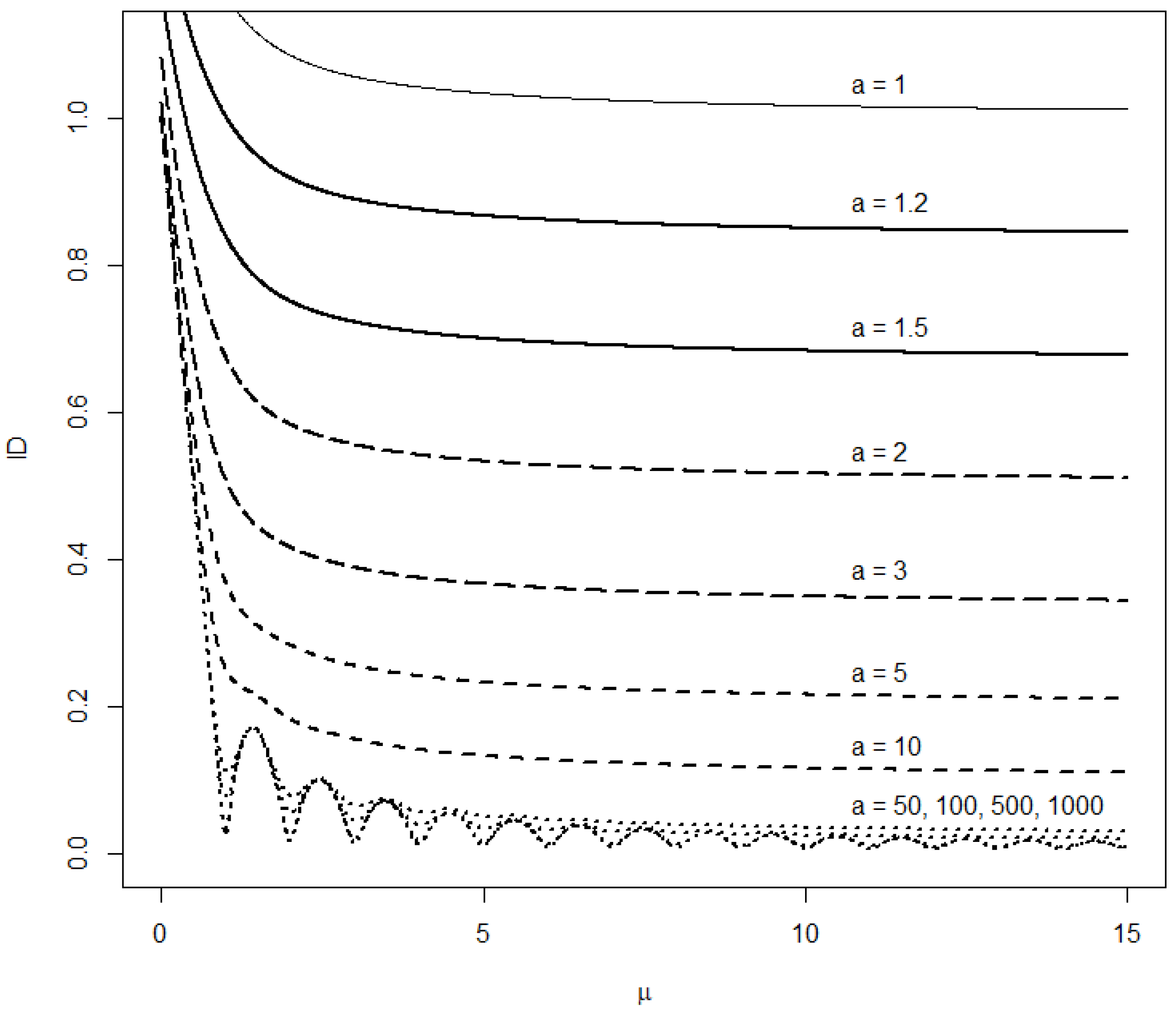
2.5. Moments and Index of Dispersion

This section presents expressions for the moments of balanced discrete distributions. We start with the first two moments since they are the most important in a count regression context.

Proposition 2

(Mean and variance). Let $X\sim \mathcal{CD}\left(\mathbf{\theta }\right)$ with mean ${\mu }_X\left(\mathbf{\theta }\right)$ and variance ${\sigma }_X^2\left(\mathbf{\theta }\right)$. The balanced discrete counterpart of X, $Y\sim \mathcal{BD}\left(\mathbf{\theta }\right)$, has mean ${\mu }_Y\left(\mathbf{\theta }\right)={\mu }_X\left(\mathbf{\theta }\right)$ and variance:

$$\begin{array}{c}\hfill {\sigma }_Y^2\left(\mathbf{\theta }\right)={\sigma }_X^2\left(\mathbf{\theta }\right)+{\zeta }_0\left(\mathbf{\theta }\right)\end{array}$$

(15)

where ${\zeta }_0\left(\mathbf{\theta }\right)={\mathrm{E}}_X\left[R\left(1-R\right)\right]$ with $R\stackrel{d}{=}X-⌊X⌋$. In addition, ${\zeta }_0\left(\mathbf{\theta }\right)$ satisfies the inequality $0<{\zeta }_0\left(\mathbf{\theta }\right)<min\left\{{\mu }_Y\left(\mathbf{\theta }\right),1/4\right\}$ and is given by the sum ${\zeta }_0\left(\mathbf{\theta }\right)={\sum }_{z=-\infty }^{\infty }{\zeta }_0(z,\mathbf{\theta })$ with:

$$\begin{array}{c}\hfill {\zeta }_0(z,\mathbf{\theta })=(2z+1){\mathrm{E}}_X\left(1,z|\mathbf{\theta }\right)-{\mathrm{E}}_X\left(2,z|\mathbf{\theta }\right)-z(z+1)H_X\left(z\right|\mathbf{\theta }).\end{array}$$

(16)

From Proposition 2, it appears that when the variance of a balanced discrete variable Y exists, it satisfies ${\sigma }_X^2\left(\mathbf{\theta }\right)<{\sigma }_Y^2\left(\mathbf{\theta }\right)<{\sigma }_X^2\left(\mathbf{\theta }\right)+min\left\{{\mu }_Y\left(\mathbf{\theta }\right),1/4\right\}$. This suggests the inexpensive approximation ${\widehat{\sigma }}_Y^2\left(\mathbf{\theta }\right)={\sigma }_X^2\left(\mathbf{\theta }\right)+min\left\{\widehat{\mu }/2,1/8\right\}$ with $|{\widehat{\sigma }}_Y^2\left(\mathbf{\theta }\right)-{\sigma }_Y^2\left(\mathbf{\theta }\right)|<min\left\{\widehat{\mu }/2,1/8\right\}$, $\widehat{\mu }$ being the mean of Y (exact or estimate). The following corollary infers the ID (index of dispersion) of a balanced discrete distribution from Proposition 2.

Corollary 1

(Index of dispersion). Let $Y\sim \mathcal{BD}\left(\mathbf{\theta }\right)$ be the balanced discrete counterpart of $X\sim \mathcal{CD}\left(\mathbf{\theta }\right)$ with cdf $F_X(·|\mathbf{\theta })$, quf $Q_X(·|\mathbf{\theta })$, expectation ${\mu }_X\left(\mathbf{\theta }\right)\ne 0$, and index of dispersion (variance-to-mean ratio) ${\mathrm{ID}}_X\left(\mathbf{\theta }\right)$. The index of dispersion ${\mathrm{ID}}_Y\left(\mathbf{\theta }\right)$ of Y satisfies:

$$\begin{array}{ccc}\hfill {\mathrm{ID}}_Y\left(\mathbf{\theta }\right)& =& {\mathrm{ID}}_X\left(\mathbf{\theta }\right)+\frac{{\zeta }_0\left(\mathbf{\theta }\right)}{{\mu }_X\left(\mathbf{\theta }\right)}\hfill \end{array}$$

(17)

$$\begin{array}{ccc}\hfill |{\mathrm{ID}}_X\left(\mathbf{\theta }\right)|& <& |{\mathrm{ID}}_Y\left(\mathbf{\theta }\right)|\le |{\mathrm{ID}}_X\left(\mathbf{\theta }\right)|+\frac{1}{4|{\mu }_X\left(\mathbf{\theta }\right)|}.\hfill \end{array}$$

(18)

Furthermore, ${\zeta }_0\left(\mathbf{\theta }\right)$ can be approximated with a tolerance $\alpha \in (0,1)$ by the truncated sum:

$$\begin{array}{ccc}\hfill {\widehat{\zeta }}_{\alpha }\left(\mathbf{\theta }\right)& =& \sum _{z=z_i}^{z_f}{\zeta }_0(z,\mathbf{\theta })\hfill \end{array}$$

(19)

where $z_i=⌊Q_X\left(\alpha /2|\mathbf{\theta }\right)⌋$, $z_f=⌊Q_X\left(1-\alpha /2|\mathbf{\theta }\right)⌋+1$ and α controls the precision of ${\widehat{\zeta }}_{\alpha }\left(\mathbf{\theta }\right)$ via $|{\widehat{\zeta }}_{\alpha }\left(\mathbf{\theta }\right)-{\zeta }_0\left(\mathbf{\theta }\right)|<1-F_X\left(z_f+1|\mathbf{\theta }\right)+F_X\left(z_i|\mathbf{\theta }\right)$.

The next proposition shows the relation between moments of balanced discrete distributions and of discrete concentrations.

Proposition 3.

Let $Y\sim \mathcal{BD}\left(\mathbf{\theta }\right)$ be the balanced discrete counterpart of $X\sim \mathcal{CD}\left(\mathbf{\theta }\right)$. The nth moment of Y satisfies for $n\in {\mathbb{N}}_{+}$:

$$\begin{array}{ccc}\hfill {\mu }_Y^{\left(n\right)}\left(\mathbf{\theta }\right)& =& {\mu }_Z^{\left(n\right)}\left(\mathbf{\theta }\right)+\sum _{i=0}^{n-1}\left(\genfrac{}{}{0pt}{}{n}{i}\right){\mu }_{ZU}^{\left(i\right)}\left(\mathbf{\theta }\right)\hfill \end{array}$$

(20)

where ${\mu }_Z^{\left(n\right)}\left(\mathbf{\theta }\right)$ is the nth moment of the discrete concentration $Z=⌊X⌋$ (Equation (3)) and ${\mu }_{ZU}^{\left(i\right)}\left(\mathbf{\theta }\right)$ is the expectation of the product of $Z^i$ and U with $U|X\sim \mathcal{BER}\left(X-Z\right)$, given by ${\mu }_{ZU}^{\left(i\right)}\left(\mathbf{\theta }\right)=-{\mu }_Z^{(i+1)}\left(\mathbf{\theta }\right)+{\sum }_{z=-\infty }^{\infty }{z}^i{\mathrm{E}}_X\left(1,z|\mathbf{\theta }\right)$.

2.6. Conditional Distributions of Latent Continuous and Binary Outcomes

Although the balanced discrete distribution was motivated by the need for mean-parameterizable flexible discrete probability distributions, it may be used to model any continuous outcome measured to fewer decimal places. In such instances, the conditional distribution and in particular the conditional mean of the underlying continuous distribution may be useful for predicting the continuous variable given an observed discrete value. In addition, since a balanced discrete variable is the observable feature of an underlying continuous outcome, a useful tool for maximum likelihood inference in complex models is the expectation-maximization algorithm [22], which handles any latent class-like model. In a Bayesian inference framework, the stochastic representation of the balanced discrete distribution can also be useful for sampling the posterior distribution of model parameters when draws from the truncated form of the continuous distribution are inexpensive. The following result provides expressions for these purposes.

Proposition 4.

Let X, U, and Y be defined as in Equation (5). Then, for $y\in \mathbb{Z}$ with probability mass $f_Y\left(y\right|\mathbf{\theta })>0$:

$$\begin{array}{ccc}\hfill f_{U|Y}\left(u|Y=y,\mathbf{\theta }\right)& =& p_y^u{\left[1-p_y\right]}^{1-u}\mathrm{for}u\in \left\{0,1\right\},\hfill \end{array}$$

(21)

$$\begin{array}{ccc}\hfill f_{X|Y}\left(x|Y=y,\mathbf{\theta }\right)& =& \frac{f_X\left(x\right|\mathbf{\theta })}{f_Y\left(y\right|\mathbf{\theta })}\left[(1-y+x)I_{(y-1,y)}\left(x\right)+(1+y-x)I_{(y,y+1)}\left(x\right)\right],\hfill \end{array}$$

(22)

and for $n\in \mathbb{R}$ such that $X^n$ is well defined in both $(y-1,y)$ and $(y,y+1)$,

$$\begin{array}{ccc}\hfill E_{X|Y}\left[X^n|Y=y,\mathbf{\theta }\right]& =& \frac{1}{f_Y\left(y\right|\mathbf{\theta })}\left[(1-y)E_X(n,y-1|\mathbf{\theta })+E_X(n+1,y-1|\mathbf{\theta })\right.\hfill \\ & & \left.+(1+y)E_X(n,y|\mathbf{\theta })-E_X(n+1,y|\mathbf{\theta })\right]\hfill \end{array}$$

(23)

where $p_y={\left[f_Y\left(y\right|\mathbf{\theta })\right]}^{-1}\left[E_X(1,y-1|\mathbf{\theta })-(y-1)H_X\left(y\right|\mathbf{\theta })\right]$ is the conditional mean (success probability) of the Bernoulli variable U given $Y=y$ and $I_{\mathbb{A}}\left(x\right)$ is the indicator function, which equals one if $x\in \mathbb{A}$ and 0 otherwise.

Note from Equation (22) that given the continuous variable, the distribution of the discrete variable does not depend on the parameter vector $\mathbf{\theta }$:

$$\begin{array}{c}\hfill f_{Y|X}\left(y|X=x,\mathbf{\theta }\right)=(1-y+x)I_{(y-1,y)}\left(x\right)+(1+y-x)I_{(y,y+1)}\left(x\right).\end{array}$$

(24)

Therefore, in the expectation-maximization algorithm framework, the maximization of the joint likelihood:

$$\begin{array}{c}\hfill f_{X,Y}\left(x,y\right)=f_{Y|X}\left(y|X=x,\mathbf{\theta }\right)f_X\left(x|\mathbf{\theta }\right)\end{array}$$

(25)

of Y and X is reduced to the maximization of the likelihood $f_X\left(x|\mathbf{\theta }\right)$ of the continuous variable X. Hence, the expectation-maximization algorithm will be appropriate for fitting a balanced discrete distribution whenever fitting the underlying continuous distribution is easy.

2.7. Link with Mean-Preserving Discretization

Recall from Equation (4) that the cdf of the mean-preserved count variable has the form:

$$\begin{array}{c}\hfill F_Y\left(y\right|\mathbf{\theta })={\int }_y^{y+1}{F}_X\left(x\right|\mathbf{\theta })dx.\end{array}$$

From the identity $\int F_X\left(x\right|\mathbf{\theta })dx=x{F}_X\left(x\right|\mathbf{\theta })-\int x{f}_X\left(x\right|\mathbf{\theta })dx$, we have:

$$\begin{array}{c}\hfill F_Y\left(y\right|\mathbf{\theta })=(y+1)F_X(y+1|\mathbf{\theta })-y{F}_X\left(y\right|\mathbf{\theta })-{\mathrm{E}}_X\left(1,y|\mathbf{\theta }\right).\end{array}$$

(26)

Then, using the identity $F_X(y+1|\mathbf{\theta })=F_X\left(y\right|\mathbf{\theta })+\left[F_X(y+1|\mathbf{\theta })-F_X\left(y\right|\mathbf{\theta })\right]$ straightforwardly results in:

$$\begin{array}{c}\hfill F_Y\left(y\right|\mathbf{\theta })=F_X\left(y\right|\mathbf{\theta })+(y+1)\left[F_X(y+1|\mathbf{\theta })-F_X\left(y\right|\mathbf{\theta })\right]-{\mathrm{E}}_X\left(1,y|\mathbf{\theta }\right),\end{array}$$

i.e., the cdf in Equation (12). Therefore, balanced discretization as defined in Equation (5) provides a generating mechanism for the mean-preserving method of [3].

3. The Balanced Discrete Gamma Family

The class of gamma distributions is a flexible class of distributions encountered in various statistical applications. This class of distributions includes as special cases the exponential, the one-parameter gamma, and up to rescaling the chi-squared distributions [23]. Chakraborty and Chakravarty [24] studied the discrete concentration of the gamma distribution with applications in biology and socio-economics. In order to allow exact inference in flexible count regression models, we apply in this section the balanced discretization method to gamma distributions. We present the balanced discrete gamma distribution under mean parametrization convenient for regression purposes and compare the distribution to the discrete concentration of the gamma distribution and to the Poisson distribution.

Let $\mathcal{G}(b,a)$ denote the gamma distribution with cdf $F_g\left(x\right|b,a)=\gamma (ax,b)$ for $x>0$, where $\gamma (x,a)={\int }_0^x{u}^{a-1}{\mathrm{e}}^{-u}du/\Gamma \left(a\right)$ is the lower incomplete gamma ratio for $(a,x)\in {\mathbb{R}}_{+}^2$ and $\Gamma \left(a\right)={\int }_0^{\infty }{u}^{a-1}{\mathrm{e}}^{-u}du$ is the gamma function. A random variable $X\sim \mathcal{G}(b,a)$ has expectation $b/a$, variance $b/\left(a^2\right)$, and nth order partial moment $E_g(n,y|b,a)={\mathrm{E}}_X\left[X^n|y\le X<y+1\right]$ given by:

$$\begin{array}{ccc}\hfill E_g(n,y|b,a)& =& \frac{\Gamma (b+n)}{a^n\Gamma \left(b\right)}\left[\gamma \left(a(y+1),b+n)\right)-\gamma \left(ay,b+n\right)\right].\hfill \end{array}$$

(27)

The one-parameter gamma distribution is obtained for $a=1$ (equidispersion) and is denoted $\mathcal{G}\left(b\right)$.

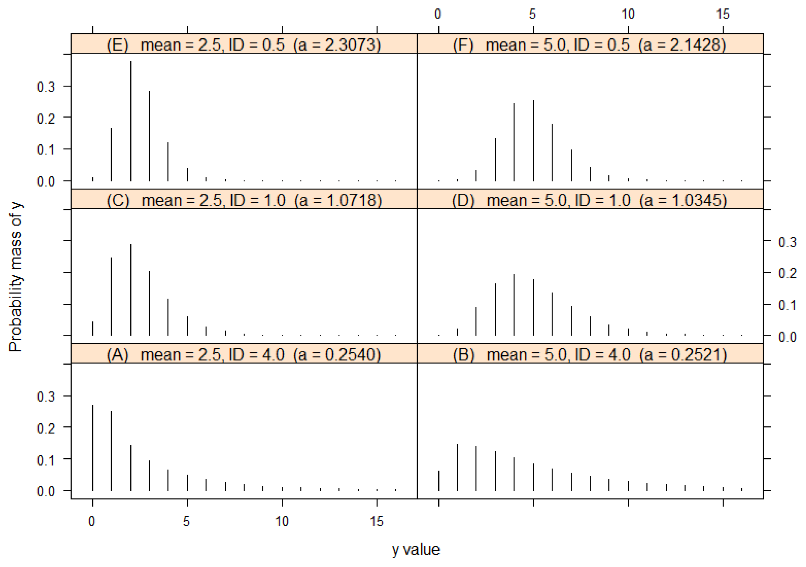
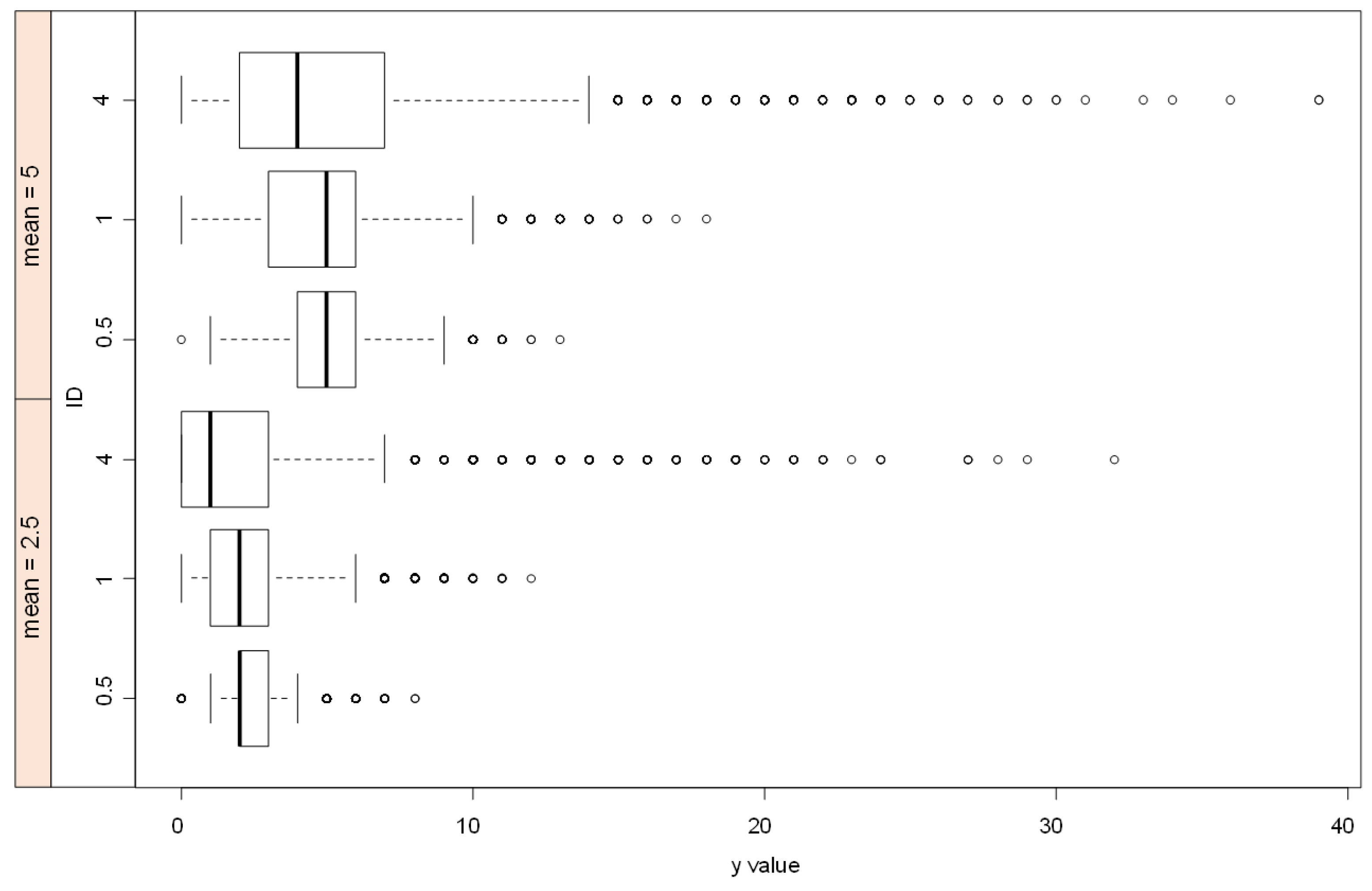
3.1. The Balanced Discrete Gamma Distribution

A count random variable with support $\mathbb{N}$ is said to follow a balanced discrete gamma distribution denoted $\mathcal{BG}(\mu ,a)$ for $(\mu ,a)\in {\mathbb{R}}_{+}^2$, if it is generated by the discretization mechanism in Equation (5) with $X\sim \mathcal{G}(a\mu ,a)$. By Proposition 2, a $\mathcal{BG}(\mu ,a)$ variable has expectation $\mu$. Using Equation (27), some properties of $\mathcal{BG}(\mu ,a)$ follow as in Corollary 2 hereafter.

Corollary 2

(Balanced discrete gamma distribution). Let $Y\sim \mathcal{BG}(\mu ,a)$, and set $b=a\mu$. Then, the pmf and the cdf of Y are respectively given for $y\in \mathbb{N}$ by:

$$\begin{array}{ccc}\hfill f_{dg}\left(y|\mu ,a\right)& =& (y-1)\gamma \left(a(y-1),b\right)-2y\gamma \left(ay,b\right)+(y+1)\gamma \left(a(y+1),b\right)\hfill \\ & & -\mu \left[\gamma \left(a(y-1),b+1\right)-2\gamma \left(ay,b+1\right)+\gamma \left(a(y+1),b+1\right)\right]\hfill \end{array}$$

(28)

$$\begin{array}{ccc}\hfill F_{dg}\left(y|\mu ,a\right)& =& (y+1)\gamma \left(a(y+1),b\right)-y\gamma \left(ay,b\right)\hfill \\ & & -\mu \left[\gamma \left(a(y+1),b+1\right)-\gamma \left(ay,b+1\right)\right];\hfill \end{array}$$

(29)

and the variance and the index of dispersion of Y are respectively given by:

$$\begin{array}{ccc}\hfill {\sigma }_{dg}^2\left(\mu ,a\right)& =& a^{-1}\mu +{\zeta }_{g_0}\left(\mu ,a\right)\hfill \end{array}$$

(30)

$$\begin{array}{ccc}\hfill {\mathrm{ID}}_{dg}\left(\mu ,a\right)& =& a^{-1}+{\mu }^{-1}{\zeta }_{g_0}\left(\mu ,a\right)\hfill \end{array}$$

(31)

where:

$$\begin{array}{ccc}\hfill {\zeta }_{g_0}\left(\mu ,a\right)& =& \sum _{z=0}^{\infty }{\zeta }_{g_0}\left(z,\mu ,a\right)\mathrm{with}\hfill \end{array}$$

(32)

$$\begin{array}{ccc}\hfill {\zeta }_{g_0}\left(z,\mu ,a\right)& =& -\mu \left(\mu +a^{-1}\right)\left[\gamma \left(a(z+1),b+2\right)-\gamma \left(az,b+2\right)\right]\hfill \\ & & \mu (2z+1)\left[\gamma \left(a(z+1),b+1\right)-\gamma \left(az,b+1\right)\right]\hfill \\ & & -z(z+1)\left[\gamma \left(a(z+1),b\right)-\gamma \left(az,b\right)\right].\hfill \end{array}$$

(33)

The pmf (28) and the cdf (29) follow by Equations (11) and (12) respectively along with Equation (27). Note that the computations of the pmf and the cdf of a balanced discrete gamma distribution only require a routine for the incomplete gamma ratio $\gamma \left(·,·\right)$, which is available in most statistical software as the cdf of the continuous gamma distribution (e.g., pgamma in the R freeware [25] and gamcdf in MATLAB [26]). The variance (30) and the index of dispersion (31) follow by Equation (15) along with Equation (27). Note that the variance term ${\zeta }_{g_0}\left(\mu ,a\right)$ in Equation (32) can be approximated via the truncation mechanism in Equation (19) with a tolerance $\alpha \in (0,1)$ as:

$$\begin{array}{ccc}\hfill {\widehat{\zeta }}_{g_{\alpha }}(\mu ,a)& =& \sum _{z=z_i}^{z_f}{\zeta }_{g_0}(z,\mu ,a)\hfill \end{array}$$

(34)

where $z_i=⌊{\gamma }^{-1}\left(\alpha /2,b\right)/a⌋$, $z_f=⌊{\gamma }^{-1}\left(1-\alpha /2,b\right)/a⌋+1$ with ${\gamma }^{-1}(·,b)$ the inverse function of the incomplete gamma ratio $\gamma \left(·,b\right)$ (available, e.g., as qgamma in R and gaminv in MATLAB).

The one-parameter BDG (balanced discrete gamma) distribution, denoted $\mathcal{BG}\left(\mu \right)$ and obtained by setting $a=1$, corresponds to a latent equidispersion mechanism and is marginally slightly overdispersed as indicated by Equation (31) with $a=1$. Setting $a={\mu }^{-1}$ produces the balanced discrete exponential distribution $\mathcal{BE}\left(\mu \right)$, which is close to the geometric distribution since the latter corresponds to the discrete concentration of the exponential distribution [27].

Figure 1 displays the probability mass function of the BDG distributions with mean values $\mu =2.5$ and $\mu =5$ (computed using Equation (28) in R). It appears that the scale parameter a controls the shape of the distribution, allowing both unimodal and reverse J shapes. It can be observed that the spread of a BDG distribution $\mathcal{BG}(\mu ,a)$ decreases with a for fixed $\mu$. The boxplots depicted in Figure 2 show that the skewness of the distribution (as measured by the difference between the mean and the median values) increases with its spread and thus decreases with a. As expected, both the length of the right tail of the distribution (Figure 1) and the probability of unusual (far from the mean and the median) observations (Figure 2) increase with the spread.

The index of dispersion, which can assume any positive value, is computed using Equation (31) in R and depicted in Figure 3 for $a\ge 1$. It can be observed in accordance with Equation (31) that for large mean values ($\mu \ge 10$), the variance-to-mean ratio is not very sensitive to $\mu$ for fixed, but not too large scale parameter values ($a<50$). This also holds for very low scales ($a<0.5$) for any mean value. Very large scales ($a\ge 50$) induce, in addition to severe underdispersion ($\mathrm{ID}<0.2$), an oscillating index of dispersion with an amplitude approaching zero as $\mu$ increases. Indeed, for large-scale values (as $a\to \infty$) and finite $\mu$, the continuous gamma distribution converges to a point mass at $\mu$. The balanced discrete gamma distribution thus converges to a binary variable, which takes the values $y=⌊\mu ⌋$ with the probability $1-(\mu -⌊\mu ⌋)$ and $y=⌊\mu ⌋+1$ with the probability $(\mu -⌊\mu ⌋)$ and has variance ${\sigma }_{dg}^2\left(\mu ,\infty \right)=(\mu -⌊\mu ⌋)(1-\mu +⌊\mu ⌋)$. The oscillating pattern in Figure 3 accordingly shows that the variance is minimal when $\mu$ is an integer and maximal when $\mu$ is a half integer. When both $\mu$ and a are large, the amplitude of the oscillations of $\mathrm{ID}$ decreases, and $\mathrm{ID}$ approaches zero, in accordance with Equation (31).

3.2. Comparison with Some Alternatives

The balanced discretization approach results from a light modification of the discrete concentration method. This section assesses on the one hand to what extent the two discretization approaches differ, considering the balanced discrete gamma (BDG) distribution case. On the other hand, the difference between the Poisson and the BDG distributions is evaluated under both latent and marginal equidispersion restrictions.

Among the miscellaneous measures proposed to assess the similarities between probability distributions, the Jensen–Shannon divergence (JSD) [28] has many desirable properties that support its use in statistics [29]. The JSD is an information theory measure given for two pmfs $q_1(·)$ and $q_2(·)$ by [28]:

$$\begin{array}{ccc}\hfill JSD\left(q_1,q_2\right)& =& K\left(q_1,q_2\right)+K\left(q_2,q_1\right)\hfill \end{array}$$

(35)

$$\begin{array}{ccc}\hfill \mathrm{where}K\left(q_1,q_2\right)& =& \sum _{y=-\infty }^{\infty }{q}_1\left(y\right){log}_2\left(\frac{q_1\left(y\right)}{0.5q_1\left(y\right)+0.5q_2\left(y\right)}\right)\hfill \end{array}$$

(36)

with the convention $q_1\left(y\right){log}_2\left(q_1\left(y\right)/(0.5q_1\left(y\right)+0.5q_2\left(y\right))\right)=0$ if $q_1\left(y\right)=0$. The JSD measures the discrepancy between $q_1(·)$ and $q_2(·)$ in bits. It is bounded as $0\le JSD\left(q_1,q_2\right)\le 2$ and is zero only if $q_1\left(y\right)=q_2\left(y\right)\forall y\in \mathbb{Z}$. The JSD values presented in this section are computed using Equation (35) using the R freeware.

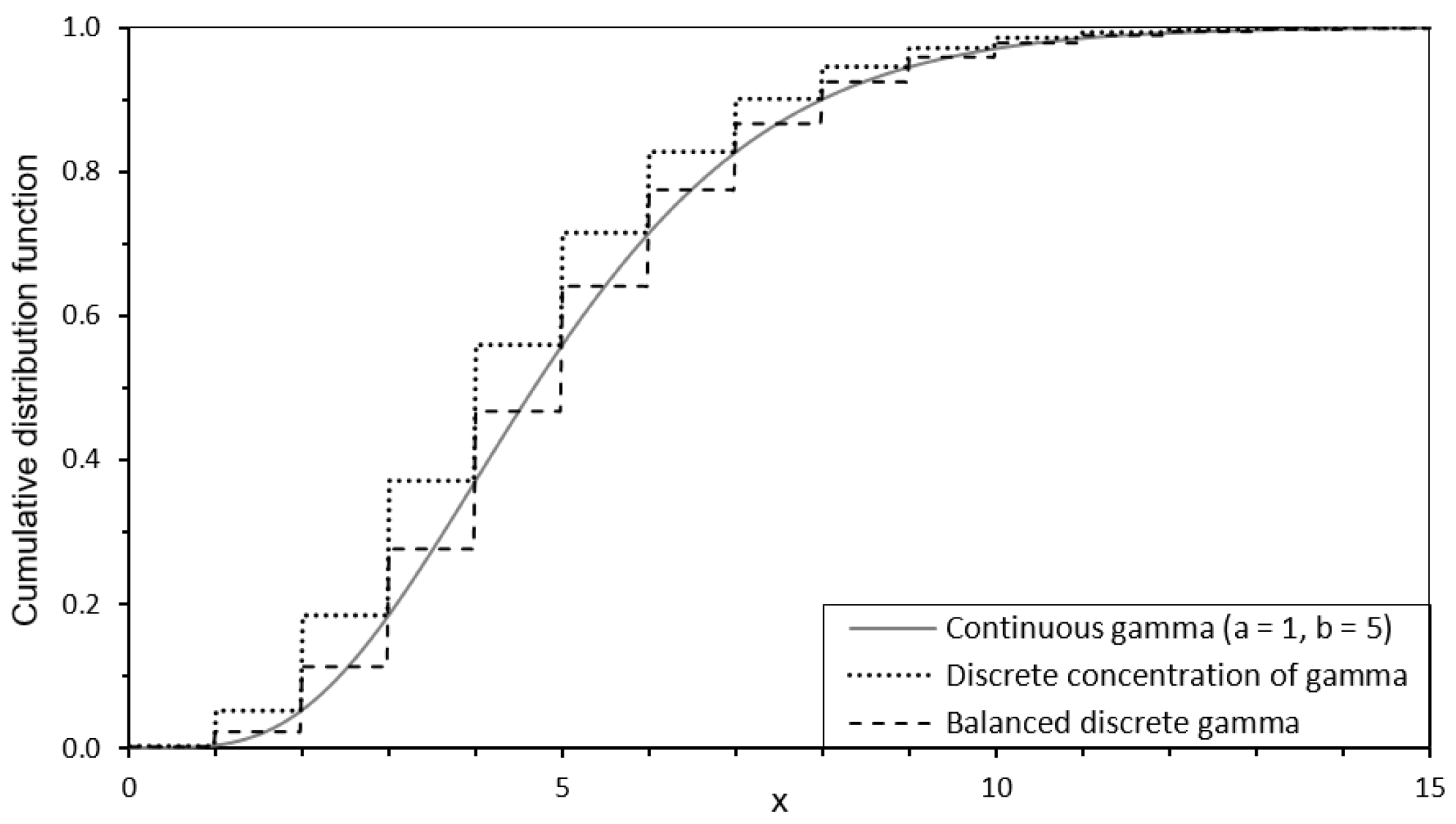
3.2.1. Balanced Discretization Versus Discrete Concentration

Figure 4 illustrates the balanced discretization method using the continuous gamma distribution with parameters $a=1$, $b=5$. Unlike the discrete concentration whose cdf lies above the continuous cdf, the balanced discrete distribution is constructed so that the continuous cdf interpolates the cdf of the balanced discrete distribution.

The curves in Figure 5A show the JSD measure between the balanced discrete gamma and the corresponding discrete concentrations for mean count values $\mu \le 30$. The selected scale values allow a wide range for the index of dispersion (ID), which roughly runs from 0.04 to 10. It can be observed that the JSD measure is relatively low ($\mathrm{JSD}<0.80$ bit) and decreases overall with the mean count (but not monotonically). In other words, the discrete concentration and balanced discretization methods produce similar discrete analogues of the considered continuous gamma distributions for large mean values. The JSD measure is especially low ($\mathrm{JSD}\le 0.10$ bit) for equidispersed and overdispersed balanced discrete gamma distributions ($a\le 1$). High discrepancy ($\mathrm{JSD}\ge 0.5$ bit) actually appears between the discrete analogues from the two discretization methods generally in underdispersion situations with a very low mean count ($\mu <1$) or large scale parameter ($a>5$, implying $\mathrm{ID}<0.45$). For very large scale values ($a\ge 30$), $\mathrm{JSD}$ becomes erratic, oscillating between minima right before the integer values of $\mu$ and maxima right after the integer values of $\mu$.

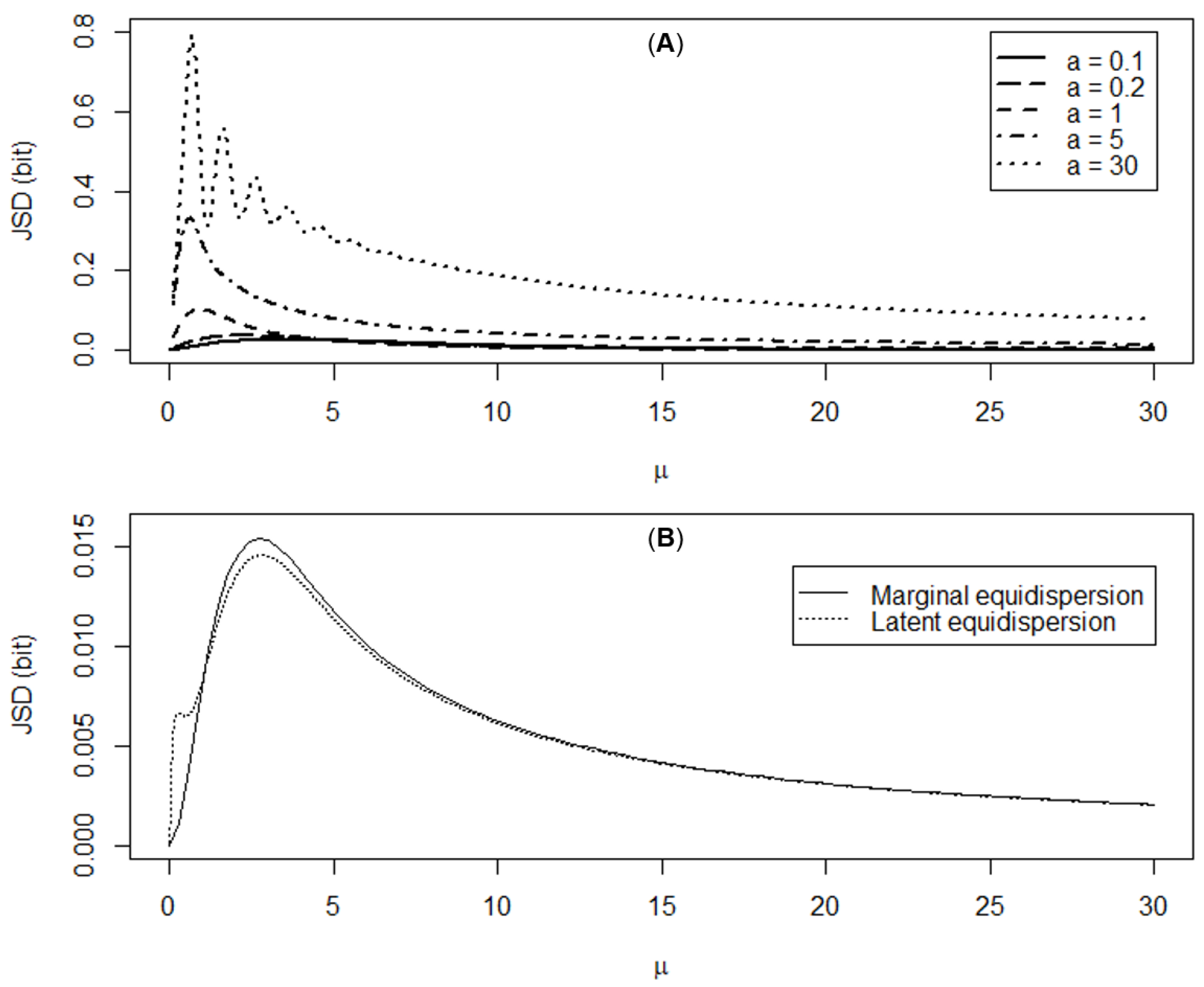
3.2.2. Distance to the Poisson Distribution under Equidispersion

The Poisson regression is the most common count regression model, which is appropriate for equidispersed count data. Although the BDG distribution does not include the Poisson distribution as a special case, the distribution can be restricted to allow equidispersion. This can be achieved by solving the nonlinear equation ${\sigma }_{dg}^2\left(\mu ,a\right)=\mu$ for a using Equation (30) (marginal equidispersion). However, the one-parameter BDG distribution $\mathcal{BG}\left(\mu \right)$ offers a conceptually insightful alternative (latent equidispersion), which is analytically tractable ($a=1$).

In order to determine which equidispersion balanced discrete gamma model (marginal vs. latent equidispersion) is the most appropriate when seeking the parsimonious flexible count regression model, the $\mathrm{JSD}$ measure was computed for fixed mean count $\mu$ between the Poisson distribution and the BDG distribution under marginal, as well as latent equidispersion restrictions. The results displayed in Figure 5B against the mean count indicate that when restricted to be equidispersed, the BDG distribution becomes similar to the Poisson distribution as per the low JSD values ($\mathrm{JSD}<0.015$ bit). It can be observed that the marginally equidispersed BDG distribution is the closest to the Poisson distribution only for a very low mean count ($\mu \le 1.1176$). For a larger mean count ($\mu >1.1176$), the one-parameter BDG distribution is closer to the Poisson distribution than the marginally equidispersed BDG distribution, although the difference becomes unnoticeable for $\mu >10$.

It appears that the one-parameter BDG distribution based count regression model will be an effective parsimonious (few parameters and more tractable) model [30] that can be fit to observed data to check the appropriateness of an equidispersion model. Therefore, while a BDG regression model will allow exact inference in flexible count modeling, testing for latent equidispersion will allow recovering a near Poisson regression model when supported by observed data.

4. Conclusions

With a view toward allowing exact inference in flexible count regression models, this work describes balanced discretization, a method for simulating and modeling integer valued data starting from a continuous random variable, through the use of a probabilistic rounding mechanism. Most of the existing alternatives were built to conserve a specific characteristic of the continuous variable, e.g., the failure rate [31] and the survival [14] functions for modeling reliability data. Our proposal preserves expectation and is thus appropriate for count regression. The method is very close to the discretizing approach of [17], which also preserves the mean value, but requires an a priori double truncation of the continuous variable and introduces a tuning parameter. Physical interpretation is an important selection criterion for choosing an appropriate discretization method [32]. As such, our proposal is motivated by a real-world generating mechanism and provides a physical interpretation for the mean-preserving method of [3]. Although balanced discrete distributions can model any count data, it may not be appropriate for aging data for which the integer part or the ceil is generally used [14] so that discrete concentrations are a better choice.

The flexibility of the balanced discrete gamma family developed from the continuous gamma distribution illustrates the potential of the balanced discretization method for capturing any level of dispersion in observed count data. In addition to flexibility, the balanced discrete gamma family turns out to be similar to the Poisson distribution when restricted to be equidispersed (marginal equidispersion) and when constructed using an equidispersed continuous gamma distribution (latent equidispersion). Based on this, we conjecture that while covering all types of dispersion, a flexible count regression model based on the balanced discrete gamma distribution will allow recovering a near Poisson distribution model when the data are Poisson distributed. Future research will target the use of the balanced discrete distribution in count regression analysis. The extension of balanced discretization to a multivariate setting is also considered to handle count data grouped by some sampling units and mixtures of count and continuous responses.

References

1. Hilbe, J.M. Negative Binomial Regression; Cambridge University Press: Cambridge, UK, 2011; p. 573. [Google Scholar]
2. Sellers, K.F.; Shmueli, G. Data dispersion: Now you see it ⋯ now you don’t. Commun. Stat. Theory Methods 2013, 42, 3134–3147. [Google Scholar] [CrossRef] [Green Version]
3. Hagmark, P.E. On construction and simulation of count data models. Math. Comput. Simul. 2008, 77, 72–80. [Google Scholar] [CrossRef]
4. Wedderburn, R.W. Quasi-likelihood functions, generalized linear models, and the Gauss—Newton method. Biometrika 1974, 61, 439–447. [Google Scholar] [CrossRef]
5. Consul, P.; Famoye, F. Generalized Poisson regression model. Commun. Stat. Theory Methods 1992, 21, 89–109. [Google Scholar] [CrossRef]
6. Bonat, W.H.; Jørgensen, B.; Kokonendji, C.C.; Hinde, J.; Demétrio, C.G. Extended Poisson–Tweedie: Properties and regression models for count data. Stat. Model. 2018, 18, 24–49. [Google Scholar] [CrossRef] [Green Version]
7. Conway, R.W.; Maxwell, W.L. A queuing model with state dependent service rates. J. Ind. Eng. 1962, 12, 132–136. [Google Scholar]
8. Efron, B. Double exponential families and their use in generalized linear regression. J. Am. Stat. Assoc. 1986, 81, 709–721. [Google Scholar] [CrossRef]
9. Zou, Y.; Geedipally, S.R.; Lord, D. Evaluating the double Poisson generalized linear model. Accid. Anal. Prev. 2013, 59, 497–505. [Google Scholar] [CrossRef] [PubMed] [Green Version]
10. Winkelmann, R. A count data model for gamma waiting times. Stat. Pap. 1996, 37, 177–187. [Google Scholar] [CrossRef]
11. Cameron, A.C.; Johansson, P. Count data regression using series expansions: With applications. J. Appl. Econom. 1997, 12, 203–223. [Google Scholar] [CrossRef] [Green Version]
12. Klakattawi, H.; Vinciotti, V.; Yu, K. A simple and adaptive dispersion regression model for count data. Entropy 2018, 20, 142. [Google Scholar] [CrossRef] [Green Version]
13. Zeviani, W.M.; Ribeiro, P.J., Jr.; Bonat, W.H.; Shimakura, S.E.; Muniz, J.A. The Gamma-count distribution in the analysis of experimental underdispersed data. J. Appl. Stat. 2014, 41, 2616–2626. [Google Scholar] [CrossRef] [Green Version]
14. Chakraborty, S. Generating discrete analogues of continuous probability distributions-A survey of methods and constructions. J. Stat. Distrib. Appl. 2015, 2, 30. [Google Scholar] [CrossRef] [Green Version]
15. Plan, E.L. Modeling and simulation of count data. CPT Pharmacomet. Syst. Pharmacol. 2014, 3, 1–12. [Google Scholar] [CrossRef] [PubMed]
16. Veraart, A.E. Modeling, simulation and inference for multivariate time series of counts using trawl processes. J. Multivar. Anal. 2019, 169, 110–129. [Google Scholar] [CrossRef] [Green Version]
17. Roy, D.; Dasgupta, T.A. A discretizing approach for evaluating reliability of complex systems under stress-strength model. IEEE Trans. Reliab. 2001, 50, 145–150. [Google Scholar] [CrossRef]
18. Hagmark, P.E. A new concept for count distributions. Stat. Probab. Lett. 2009, 79, 1120–1124. [Google Scholar] [CrossRef] [Green Version]
19. Hagmark, P.E. An Exceptional Generalization of the Poisson Distribution. Open J. Stat. 2012, 2, 313–318. [Google Scholar] [CrossRef] [Green Version]
20. Chakraborty, S. A New Discrete Distribution Related to Generalized Gamma Distribution and Its Properties. Commun. Stat. Theory Methods 2013, 44, 1691–1705. [Google Scholar] [CrossRef]
21. Holland, B.S. Some Results on the discretization of continuous probability distributions. Technometrics 1975, 17, 333–339. [Google Scholar] [CrossRef]
22. Dempster, A.P.; Laird, N.M.; Rubin, D.B. Maximum likelihood from incomplete data via the EM algorithm. J. R. Stat. Soc. Ser. B (Methodol.) 1977, 39, 1–38. [Google Scholar] [CrossRef]
23. Lawless, J.F. Statistical Models and Methods for Lifetime Data, 2nd ed.; Wiley Series in Probability and Statistics; Wiley-Interscience: New York, NY, USA, 2002. [Google Scholar]
24. Chakraborty, S.; Chakravarty, D. Discrete Gamma Distributions: Properties and Parameter Estimations. Commun. Stat. Theory Methods 2012, 41, 3301–3324. [Google Scholar] [CrossRef]
25. R Core Team. R: A Language and Environment for Statistical Computing; R Foundation for Statistical Computing: Vienna, Austria, 2020. [Google Scholar]
26. MATLAB. Version 9.0.0 (R2016a); The MathWorks Inc.: Natick, MA, USA, 2016. [Google Scholar]
27. Roy, D. Reliability measures in the discrete bivariate set-up and related characterization results for a bivariate geometric distribution. J. Multivar. Anal. 1993, 46, 362–373. [Google Scholar] [CrossRef] [Green Version]
28. Lin, J. Divergence measures based on the Shannon entropy. IEEE Trans. Inf. Theory 1991, 37, 145–151. [Google Scholar] [CrossRef] [Green Version]
29. Zhang, X.; Delpha, C.; Diallo, D. Performance of Jensen Shannon Divergence in Incipient Fault Detection and Estimation. In Proceedings of the ICASSP 2019, 2019 IEEE International Conference on Acoustics, Speech and Signal Processing (ICASSP), Brighton, UK, 12–17 May 2019; pp. 2742–2746. [Google Scholar]
30. Daganzo, C.F.; Gayah, V.V.; Gonzales, E.J. The potential of parsimonious models for understanding large scale transportation systems and answering big picture questions. EURO J. Transp. Logist. 2012, 1, 47–65. [Google Scholar] [CrossRef] [Green Version]
31. Roy, D.; Ghosh, T. A new discretization approach with application in reliability estimation. IEEE Trans. Reliab. 2009, 58, 456–461. [Google Scholar] [CrossRef]
32. Bracquemond, C.; Gaudoin, O. A survey on discrete lifetime distributions. Int. J. Reliab. Qual. Saf. Eng. 2003, 10, 69–98. [Google Scholar] [CrossRef]
33. Kaehler, J. Laws of iterated expectations for higher order central moments. Stat. Pap. 1990, 31, 295–299. [Google Scholar] [CrossRef]
Figure 1. Probability mass plots for the balanced discrete gamma distributions with mean values μ = 2.5 (left panel) and μ = 5 (right panel) and scales a selected to yield an index of dispersion (ID, variance-to-mean ratio) of ID = 4 (bottom row), ID = 1 (central row), and ID = 0.5 (top row).
Mathematics 09 00555 g001
Figure 2. Box plots for the balanced discrete gamma distributions with mean values μ = 2.5 and μ = 5 and an index of dispersion (ID, variance-to-mean ratio) of ID = 4, ID = 1, and ID = 0.5. The thick vertical bar inside the interquartile range (i.e., the rectangular box that has sides that are 25% (left side) and 75% (right side) quartiles) is the median of the distribution.
Mathematics 09 00555 g002
Figure 3. Index of dispersion (ID, variance-to-mean ratio) of the balanced discrete gamma distribution against the mean value ( μ ) for selected scale parameter (a) values in the range 1 , 1000 mostly corresponding to equidispersion and underdispersion ( 0 < ID 1 ).
Mathematics 09 00555 g003
Figure 4. Comparison of the cumulative distribution functions of the balanced discrete gamma and discrete concentration of gamma distributions based on a continuous gamma distribution with scale a = 1 and shape b = 5 .
Mathematics 09 00555 g004
Figure 5. Jensen–Shannon divergence (JSD in bit) measured between the balanced discrete gamma (BDG) distribution and the corresponding discrete concentration (A) and between the Poisson and the BDG distributions under both latent equidispersion (one-parameter BDG distribution) and marginal equidispersion (unit variance-to-mean ratio) restrictions (B), against the mean value ( μ ).
Mathematics 09 00555 g005
Publisher’s Note: MDPI stays neutral with regard to jurisdictional claims in published maps and institutional affiliations.