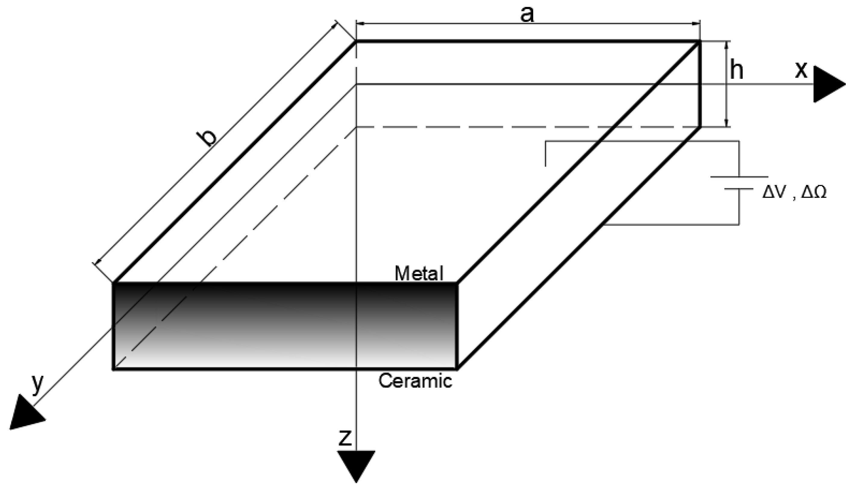
Figure 1.
Functionally graded plate with applied electric and magnetic potentials .
Figure 1.
Functionally graded plate with applied electric and magnetic potentials .
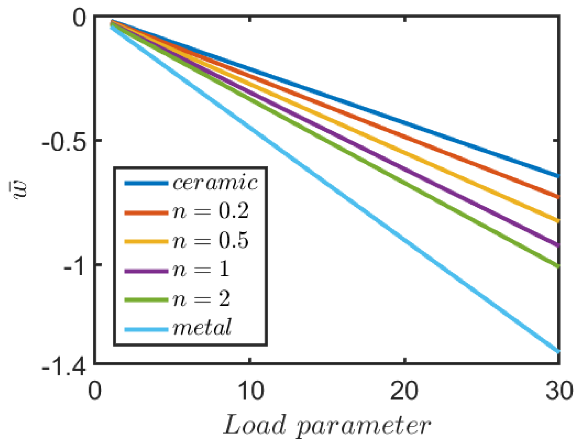
Figure 2.
Displacement of middle point of a FG square plate composed of Al/ZrO for different values of .
Figure 2.
Displacement of middle point of a FG square plate composed of Al/ZrO for different values of .
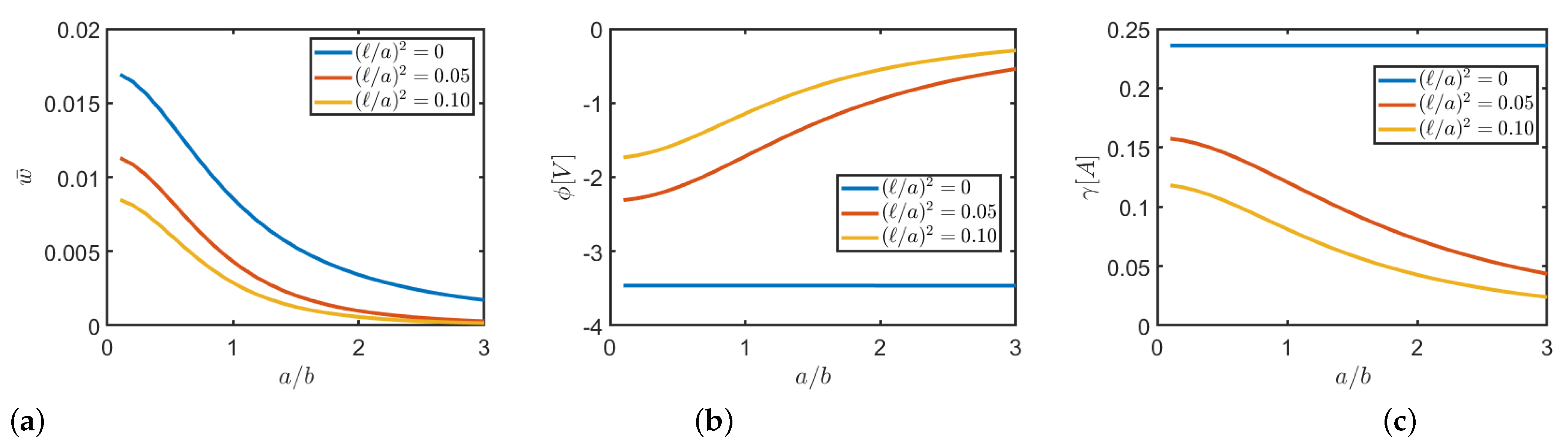
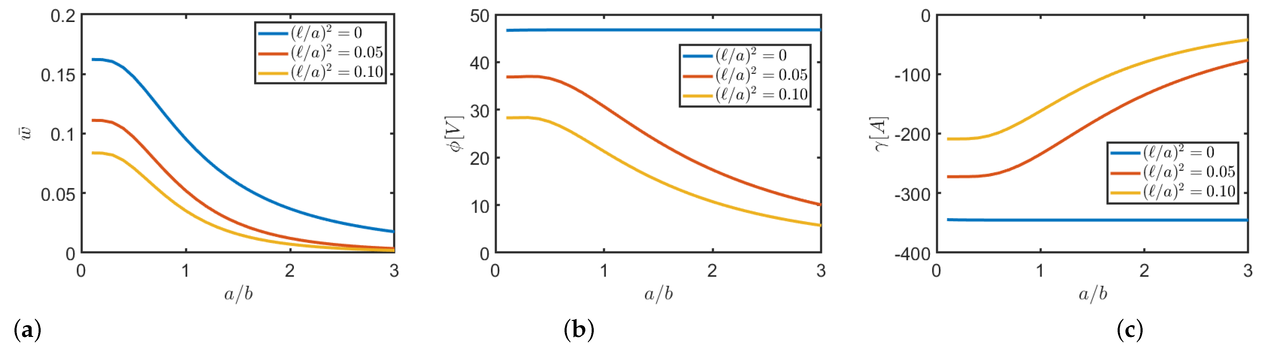
Figure 3.
Graphs of displacement (a) electric (b) and magnetic (c) potential, in the point to vary of ratio and for different values of nonlocal parameter and for (SDL; N/m, K, C/m, Wb/m).
Figure 3.
Graphs of displacement (a) electric (b) and magnetic (c) potential, in the point to vary of ratio and for different values of nonlocal parameter and for (SDL; N/m, K, C/m, Wb/m).
Figure 4.
Graphs of displacement (a) electric (b) and magnetic (c) potential, in the point to vary of ratio and for different values of nonlocal parameter and for . (SDL; N/m, K, K, C/m, Wb/m)
Figure 4.
Graphs of displacement (a) electric (b) and magnetic (c) potential, in the point to vary of ratio and for different values of nonlocal parameter and for . (SDL; N/m, K, K, C/m, Wb/m)
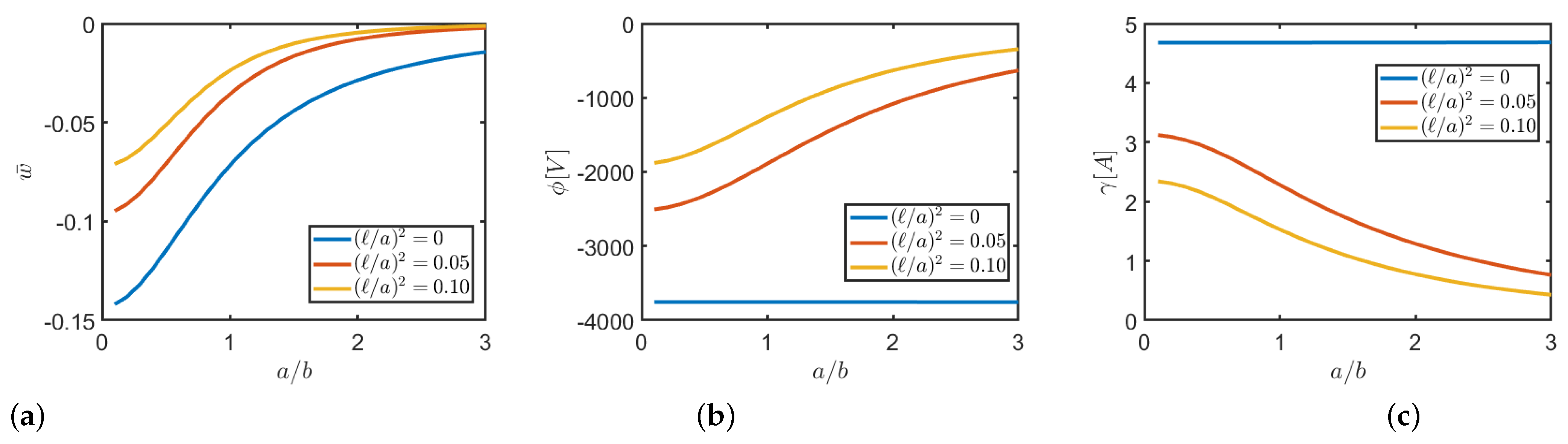
Figure 5.
Graphs of displacement (a) electric (b) and magnetic (c) potential, in the point to vary of ratio and for different values of nonlocal parameter and for . (SDL; N/m, K, C/m, Wb/m)
Figure 5.
Graphs of displacement (a) electric (b) and magnetic (c) potential, in the point to vary of ratio and for different values of nonlocal parameter and for . (SDL; N/m, K, C/m, Wb/m)
Figure 6.
Graphs of displacement (a) electric (b) and magnetic (c) potential, in the point to vary of and for different values of nonlocal parameter and for . (SDL; N/m, K, C/m, Wb/m)
Figure 6.
Graphs of displacement (a) electric (b) and magnetic (c) potential, in the point to vary of and for different values of nonlocal parameter and for . (SDL; N/m, K, C/m, Wb/m)
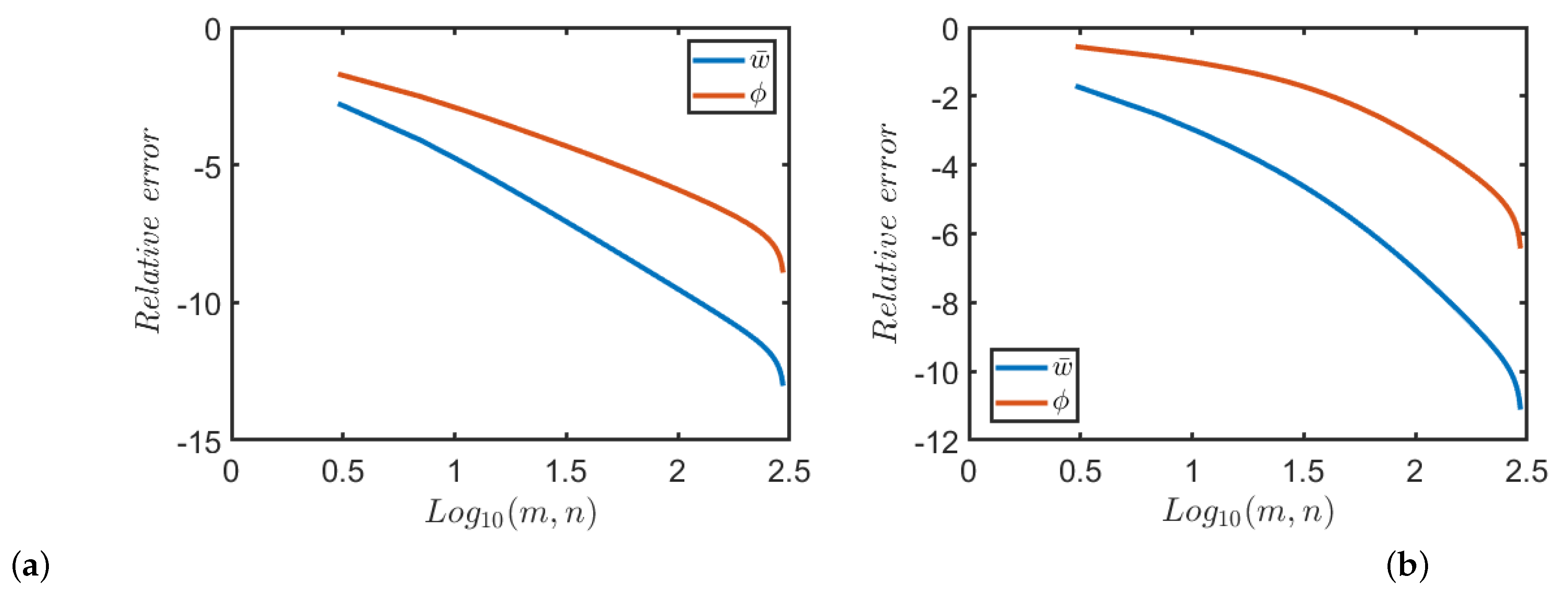
Figure 7.
Convergence of the relative error on the displacement and potential at a square plate central point by increasing for: (a) uniformly distributed mechanical load only; (b) uniformly distributed thermal load only.
Figure 7.
Convergence of the relative error on the displacement and potential at a square plate central point by increasing for: (a) uniformly distributed mechanical load only; (b) uniformly distributed thermal load only.
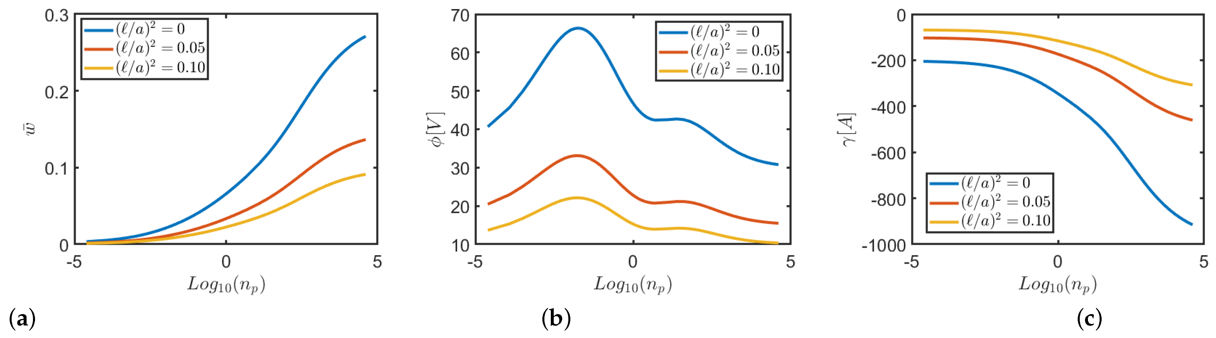
Figure 8.
Displacement (a) electric (b) and magnetic (c) potential, at the central point by varying and for different nonlocal parameters with (UDL; N/m, K, C/m, Wb/m).
Figure 8.
Displacement (a) electric (b) and magnetic (c) potential, at the central point by varying and for different nonlocal parameters with (UDL; N/m, K, C/m, Wb/m).
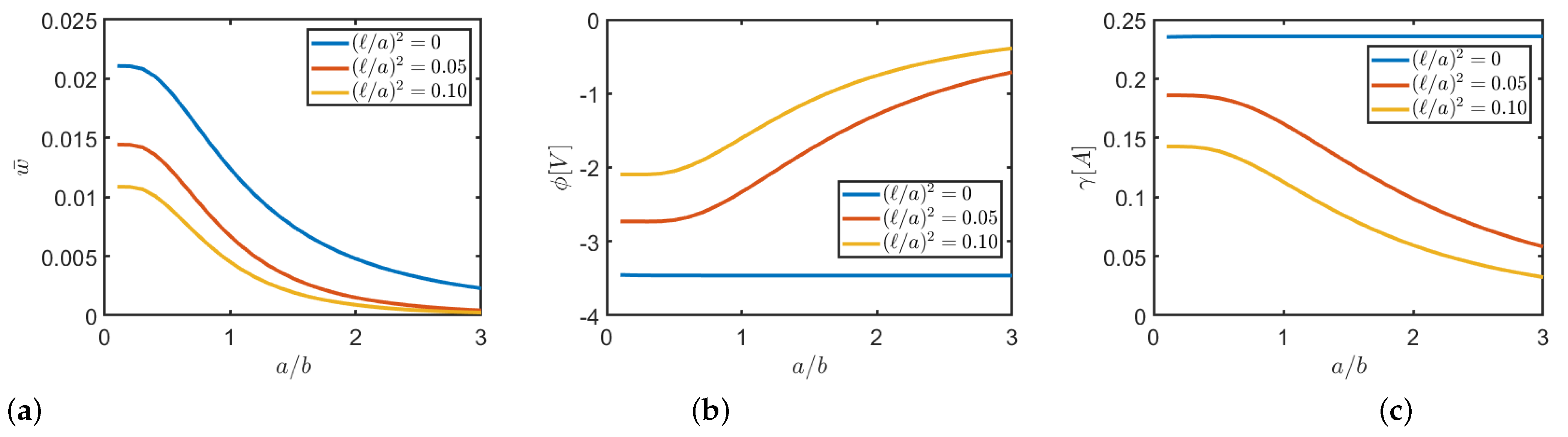
Figure 9.
Displacement (a) electric (b) and magnetic (c) potential, at the central point by varying ratio and for different nonlocal parameter with (UDL; N/m, K, K, C/m, Wb/m).
Figure 9.
Displacement (a) electric (b) and magnetic (c) potential, at the central point by varying ratio and for different nonlocal parameter with (UDL; N/m, K, K, C/m, Wb/m).
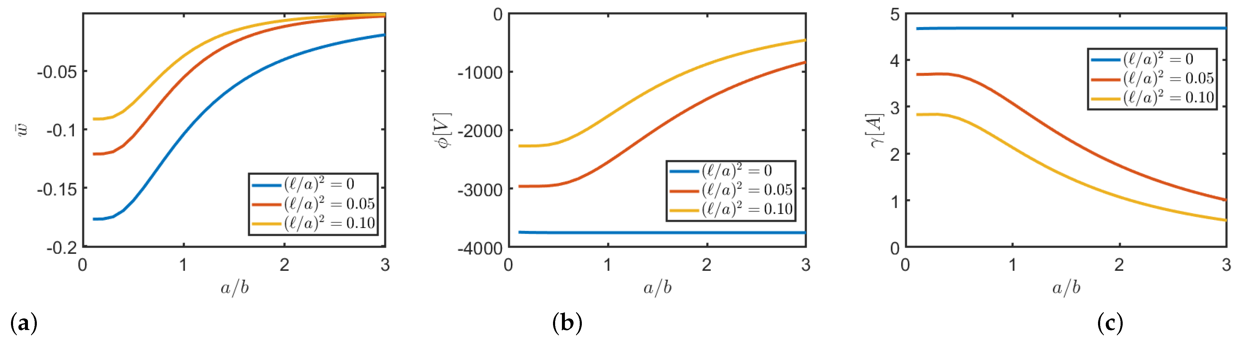
Figure 10.
Graphs of displacement (a) electric (b) and magnetic (c) potential, in the point to vary of ratio and for different values of nonlocal parameter and for . (UDL; N/m, K, C/m, Wb/m).
Figure 10.
Graphs of displacement (a) electric (b) and magnetic (c) potential, in the point to vary of ratio and for different values of nonlocal parameter and for . (UDL; N/m, K, C/m, Wb/m).
Figure 11.
Graphs of displacement (a) electric (b) and magnetic (c) potential, in the point to vary of ratio and for different values of nonlocal parameter and for . (UDL; N/m, K, C/m, Wb/m).
Figure 11.
Graphs of displacement (a) electric (b) and magnetic (c) potential, in the point to vary of ratio and for different values of nonlocal parameter and for . (UDL; N/m, K, C/m, Wb/m).
Table 1.
Piezo-electro-magnetic-thermal properties of materials BaTiO and CoFeO.
Table 1.
Piezo-electro-magnetic-thermal properties of materials BaTiO and CoFeO.
| | | BaTiO | CoFeO |
|---|
| [GPa] | 166 | 286 |
| | 166 | 286 |
| | 162 | 269.5 |
| | 78 | 170.5 |
| | 78 | 170.5 |
| | 77 | 173 |
| | 43 | 45.3 |
| | 43 | 45.3 |
| | 44.5 | 56.5 |
| [C/m] | −4.4 | 0 |
| | −4.4 | 0 |
| | 18.6 | 0 |
| [N/A·m] | 0 | 580.3 |
| | 0 | 580.3 |
| | 0 | 699.7 |
| [C/N·m] | 11.2 | 0.08 |
| | 11.2 | 0.08 |
| | 12.6 | 0.093 |
| [s/m] | 0 | 0 |
| [N·s/C] | 5 | −590 |
| | 5 | −590 |
| | 10 | 157 |
| [ C/m K] | 0 | 0 |
| | −11.4 | 0 |
| [ Wb/m K] | 0 | 0 |
| | 0 | −36.2 |
| [K] | 15.8 | 10 |
| [kg/m] | 5300 | 5800 |
Table 2.
Displacement , electric and magnetic potential and , of a square nanoplate in central point for different values of nonlocal parameter and (SDL; N/m, K, C/m, Wb/m).
Table 2.
Displacement , electric and magnetic potential and , of a square nanoplate in central point for different values of nonlocal parameter and (SDL; N/m, K, C/m, Wb/m).
| | | [V] | [A] |
|---|
| 1 | 0 | 0.01994 | −7.1675 | 0.6580 |
| | 0.05 | 0.01004 | −3.5647 | 0.3349 |
| | 0.10 | 0.00671 | −2.3721 | 0.2246 |
| 0.5 | 0 | 0.02067 | −11.463 | 0.4636 |
| | 0.05 | 0.01040 | −5.7348 | 0.2359 |
| | 0.10 | 0.00695 | −3.8236 | 0.1582 |
| 2 | 0 | 0.01929 | −4.7860 | 0.8932 |
| | 0.05 | 0.00971 | −2.3734 | 0.4531 |
| | 0.10 | 0.00649 | −1.5779 | 0.3036 |
Table 3.
Displacement , electric and magnetic potential and , of a square nanoplate in central point for different values of nonlocal parameter and . (SDL; N/m, K, K, C/m, Wb/m).
Table 3.
Displacement , electric and magnetic potential and , of a square nanoplate in central point for different values of nonlocal parameter and . (SDL; N/m, K, K, C/m, Wb/m).
| | | [V] | [A] |
|---|
| 1 | 0 | 0.00855 | −3.4621 | 0.2359 |
| | 0.05 | 0.00430 | −1.7194 | 0.1208 |
| | 0.10 | 0.00287 | −1.1435 | 0.0812 |
| 0.5 | 0 | 0.00898 | −5.4569 | 0.1739 |
| | 0.05 | 0.00452 | −2.7300 | 0.0888 |
| | 0.10 | 0.00302 | −1.8201 | 0.0595 |
| 2 | 0 | 0.00819 | −2.3699 | 0.3132 |
| | 0.05 | 0.00412 | −1.1716 | 0.1598 |
| | 0.10 | 0.00275 | −0.7781 | 0.1073 |
Table 4.
Displacement , electric and magnetic potential and , of a square nanoplate in central point for different values of nonlocal parameter and . (SDL; N/m, K, C/m, Wb/m).
Table 4.
Displacement , electric and magnetic potential and , of a square nanoplate in central point for different values of nonlocal parameter and . (SDL; N/m, K, C/m, Wb/m).
| | | [ V] | [A] |
|---|
| 1 | 0 | −0.07168 | −3.7535 | 4.6774 |
| | 0.05 | −0.03565 | −1.8899 | 2.2793 |
| | 0.10 | −0.02372 | −1.2626 | 1.5288 |
| 0.5 | 0 | −0.11463 | −4.6931 | 5.6947 |
| | 0.05 | −0.05735 | −2.3627 | 2.8018 |
| | 0.10 | −0.03824 | −1.5786 | 1.8745 |
| 2 | 0 | −0.04786 | −3.2178 | 4.2379 |
| | 0.05 | −0.02373 | −1.6199 | 2.0733 |
| | 0.10 | −0.01578 | −1.0823 | 1.3924 |
Table 5.
Displacement , electric and magnetic potential and , of a square nanoplate in central point for different values of nonlocal parameter and . (SDL; N/m, K, C/m, Wb/m).
Table 5.
Displacement , electric and magnetic potential and , of a square nanoplate in central point for different values of nonlocal parameter and . (SDL; N/m, K, C/m, Wb/m).
| | | [10 V] | [ A] |
|---|
| 1 | 0 | 0.06580 | 4.6773 | −3.4533 |
| | 0.05 | 0.03349 | 2.2793 | −1.7383 |
| | 0.10 | 0.02246 | 1.5288 | −1.1612 |
| 0.5 | 0 | 0.04636 | 5.6947 | −2.9196 |
| | 0.05 | 0.02359 | 2.8018 | −1.4696 |
| | 0.10 | 0.01582 | 1.8744 | −0.9818 |
| 2 | 0 | 0.08932 | 4.2379 | −4.0778 |
| | 0.05 | 0.04531 | 2.0733 | −2.0525 |
| | 0.10 | 0.03036 | 1.3924 | −1.3712 |
Table 6.
Displacement , electric and magnetic potential and , of a square nanoplate in central point for different values of nonlocal parameter and (UDL; N/m, K, C/m, Wb/m).
Table 6.
Displacement , electric and magnetic potential and , of a square nanoplate in central point for different values of nonlocal parameter and (UDL; N/m, K, C/m, Wb/m).
| | | [V] | [A] |
|---|
| 1 | 0 | 0.03156 | −10.413 | 0.9571 |
| | 0.05 | 0.01614 | −5.5579 | 0.5214 |
| | 0.10 | 0.01080 | −3.7245 | 0.3523 |
| 0.5 | 0 | 0.03271 | −16.668 | 0.6744 |
| | 0.05 | 0.01672 | −8.9377 | 0.3672 |
| | 0.10 | 0.01119 | −6.0017 | 0.2481 |
| 2 | 0 | 0.03054 | −6.9616 | 1.2988 |
| | 0.05 | 0.01561 | −3.7011 | 0.7055 |
| | 0.10 | 0.01044 | −2.4779 | 0.4761 |
Table 7.
Displacement , electric and magnetic potential and , of a square nanoplate at the central point for different values of nonlocal parameter and (UDL; N/m, , K, C/m, Wb/m).
Table 7.
Displacement , electric and magnetic potential and , of a square nanoplate at the central point for different values of nonlocal parameter and (UDL; N/m, , K, C/m, Wb/m).
| | | [V] | [A] |
|---|
| 1 | 0 | 0.01243 | −3.4601 | 0.2357 |
| | 0.05 | 0.00670 | −2.3305 | 0.1620 |
| | 0.10 | 0.00451 | −1.6021 | 0.1128 |
| 0.5 | 0 | 0.01306 | −5.4536 | 0.1738 |
| | 0.05 | 0.00704 | −3.6912 | 0.1192 |
| | 0.10 | 0.00474 | −2.5452 | 0.0829 |
| 2 | 0 | 0.01191 | −2.3686 | 0.3129 |
| | 0.05 | 0.00642 | −1.5904 | 0.2146 |
| | 0.10 | 0.00432 | −1.0914 | 0.1492 |
Table 8.
Displacement , electric and magnetic potential and , of a square nanoplate in central point for different values of nonlocal parameter and (UDL; N/m, K, C/m, Wb/m).
Table 8.
Displacement , electric and magnetic potential and , of a square nanoplate in central point for different values of nonlocal parameter and (UDL; N/m, K, C/m, Wb/m).
| | | [10 V] | [A] |
|---|
| 1 | 0 | −0.10421 | −3.7513 | 4.6753 |
| | 0.05 | −0.05558 | −2.5500 | 3.0680 |
| | 0.10 | −0.03725 | −1.7627 | 2.1258 |
| 0.5 | 0 | −0.16647 | −4.6922 | 5.6941 |
| | 0.05 | −0.08938 | −3.1879 | 3.7784 |
| | 0.10 | −0.06002 | −2.2038 | 2.6124 |
| 2 | 0 | −0.06950 | −3.2171 | 4.2377 |
| | 0.05 | −0.03701 | −2.1859 | 2.7877 |
| | 0.10 | −0.02478 | −1.5110 | 1.9346 |
Table 9.
Displacement , electric and magnetic potential and , of a square nanoplate in central point for different values of nonlocal parameter and . (UDL; N/m, K, C/m, Wb/m).
Table 9.
Displacement , electric and magnetic potential and , of a square nanoplate in central point for different values of nonlocal parameter and . (UDL; N/m, K, C/m, Wb/m).
| | | [10 V] | [10 A] |
|---|
| 1 | 0 | 0.09568 | 4.6753 | −3.4507 |
| | 0.05 | 0.05214 | 3.0680 | −2.3456 |
| | 0.10 | 0.03523 | 2.1258 | −1.6213 |
| 0.5 | 0 | 0.06733 | 5.6941 | −2.9191 |
| | 0.05 | 0.03672 | 3.7784 | −1.9830 |
| | 0.10 | 0.02481 | 2.6124 | −1.3707 |
| 2 | 0 | 0.12971 | 4.2377 | −4.0772 |
| | 0.05 | 0.07055 | 2.7877 | −2.7697 |
| | 0.10 | 0.04761 | 1.9346 | −1.9144 |


