
Optimization and Simulation of Dynamic Performance of Production–Inventory Systems with Multivariable Controls


1
Department of Control and System Engineering, University of Technology, Al-Wehda Neighborhood, Baghdad 10066, Iraq
2
School of Engineering and Technology, Central Queensland University, Bruce Highway, North Rockhampton, QLD 4702, Australia
*
Author to whom correspondence should be addressed.
Mathematics 2021, 9(5), 568; https://0-doi-org.brum.beds.ac.uk/10.3390/math9050568
Submission received: 29 January 2021
/
Revised: 28 February 2021
/
Accepted: 2 March 2021
/
Published: 7 March 2021
(This article belongs to the Special Issue Multivariable Optimization by Intelligent and Numerical Modelling and Simulation)
Abstract
:The production–inventory system is a problem of multivariable input and multivariant output in mathematics. Selecting the best system control parameters is a crucial managerial decision to achieve and dynamically maintain an optimal performance in terms of balancing the order rate and stock level under dynamic influence of many factors affecting the system operations. The dynamic performance of the popular APIOBPCS model and the newly modified 2APIOBPCS model for optimal control of production–inventory systems is examined in the study. This examination is based on the leveled ground with a new simulation scheme that incorporates a designated multi-objective particle swarm optimization (MOPSO) algorithm into the simulation, which enables the optimal set of system control parameters to be selected for achieving the situational best possible performance of the production–inventory system under study. The dynamic performance is measured by the variance ratio between the order rate and the sales rate related to the bullwhip effect, and the integral of absolute error related to the inventory responsiveness in response to a random customer demand. Our simulation indicates that the 2APIOBPCS model performed better than or at least no worse than, and more robust than the APIOBPCS model under different conditions.
1. Introduction
Simulation of a production–inventory system, even the simplest model comprising one manufacturer and one retailer, is a problem of multivariable input and multivariant output in mathematics. The demand (related to new order rate) and the supply or stock level (related to customer satisfaction) must be balanced under the dynamic influence of many factors affecting the system operations [1]. A low level of stock may lead to an increase in customer dissatisfaction and even loss of business opportunities to other competitors. An over exaggerated order rate may lead to over supply that reduces the financial flexibility or could drive down the sale price for the retailer. For example, Cisco encountered $2.2 billion in overstocked inventory due to an imbalance between supply and demand in May 2001 [2]. Sony Electronics faced an excessive production cost because of an over-anticipation of the demand for PlayStation®3 [3]. Either way, the production–inventory system would not be operating at a desired status for both profit generation and customer satisfaction.
Overstocking is mainly caused by the “bullwhip” effect in the production–inventory system, which is the scenario where orders to the suppliers tend to have larger fluctuations than sales to the buyers [4]. Holweg et al. [5] found that the actual demand signal from the customers in a supermarket for a soft drink was amplified many times before it reached the soft drink supplier. As no system is perfect all the time, industries have to cope with real-world bullwhip, not just a 1-to-2 amplification but a 1-to-20 or higher amplification [6]. Production–inventory systems are also subject to a variety of sources of uncertainties, such as unpredicted delay in manufacturing [7]. These combined impacts can affect the dynamic performance of any production–inventory system. Therefore, studying the dynamic control of production–inventory systems for achieving optimal performance under various uncertainties has been attempted with various models and/or methods by researchers in the world [1,4,6,7,8,9,10].
Among these models and/or methods, control theory with feedback mechanisms has become a popular choice to analyze and simulate production–inventory systems through different mathematical tools, such as Laplace transforms, Z-transforms, transfer functions, block diagrams and frequency analysis, and numerous studies have been conducted in this space [8,9,10,11,12]. The inventory and order based production control system (IOBPCS) model proposed by Towill [13] has been recognized as a common framework for modeling the control of a production–inventory system. John et al. [14] made an important extension to the IOBPCS model by including the work-in-process (WIP) feedback and proposed the automatic pipeline, inventory, and order based production control system (APIOBPCS) model, which has been widely used for modelling production–inventory systems since then [15,16,17,18,19].
In a new project started from 2017, the authors have attempted to expend the classic APIOBPCS model to a new model named two automatic pipeline inventory and order based production control system (2APIOBPCS) by incorporating the completion production rate into the production–inventory control system so as to mitigate uncertainties in manufacturing for the system modelling [20,21,22]. Our first outcome from this project produced a comprehensive literature review on the applications of classical and modern control theory to production–inventory problems [20]. The second output was mainly focused on deriving the mathematical formulation of the 2APIOBPCS model in the state space by Laplace transforms and demonstrating its stability and convergence with respect to the APIOBPCS model [21]. As both the APIOBPCS and 2APIOBPCS models represent complicated systems with more control parameters, choosing the control parameters used to be experience-based. There is a need to find an intelligent way to deal with the selection of the control parameters to achieve the optimal outcomes. The third study aimed at adopting the multi-objective particle swarm optimization (MOPSO) for selecting the best system parameters to achieve optimal control for the production–inventory systems, with a focus on simulating the well-regarded APIOBPCS model as a benchmark [22].
However, an integrated solution for the 2APIOBPCS model and its performance in dynamic control of a production–inventory system has not been systematically examined and compared to the APIOBPCS model to demonstrate its credibility and usefulness for potential industry adoption. The purpose of this work is to fill this gap by simulating the dynamic performances of these two models under different scenarios, including the consistency between the order and the production (lead time) and flexibility in production capacity for a simple production–inventory system.
The rest of this study is organized as follows. Section 2 provides a brief review of the APIOBPCS and 2APIOBPCS models and a summary of their mathematical formulations for simulations, including the performance metrics. Section 3 details the procedure of simulation and experimental considerations. Section 4 presents the simulation outcomes incorporated with comparisons and discussions. Section 5 concludes the study by summarizing the main findings of this work.
2. Background Information of the Control Models for Production-Inventory Systems
2.1. A Beief Review of the the APIOPBCS and 2APIOPBCS Models
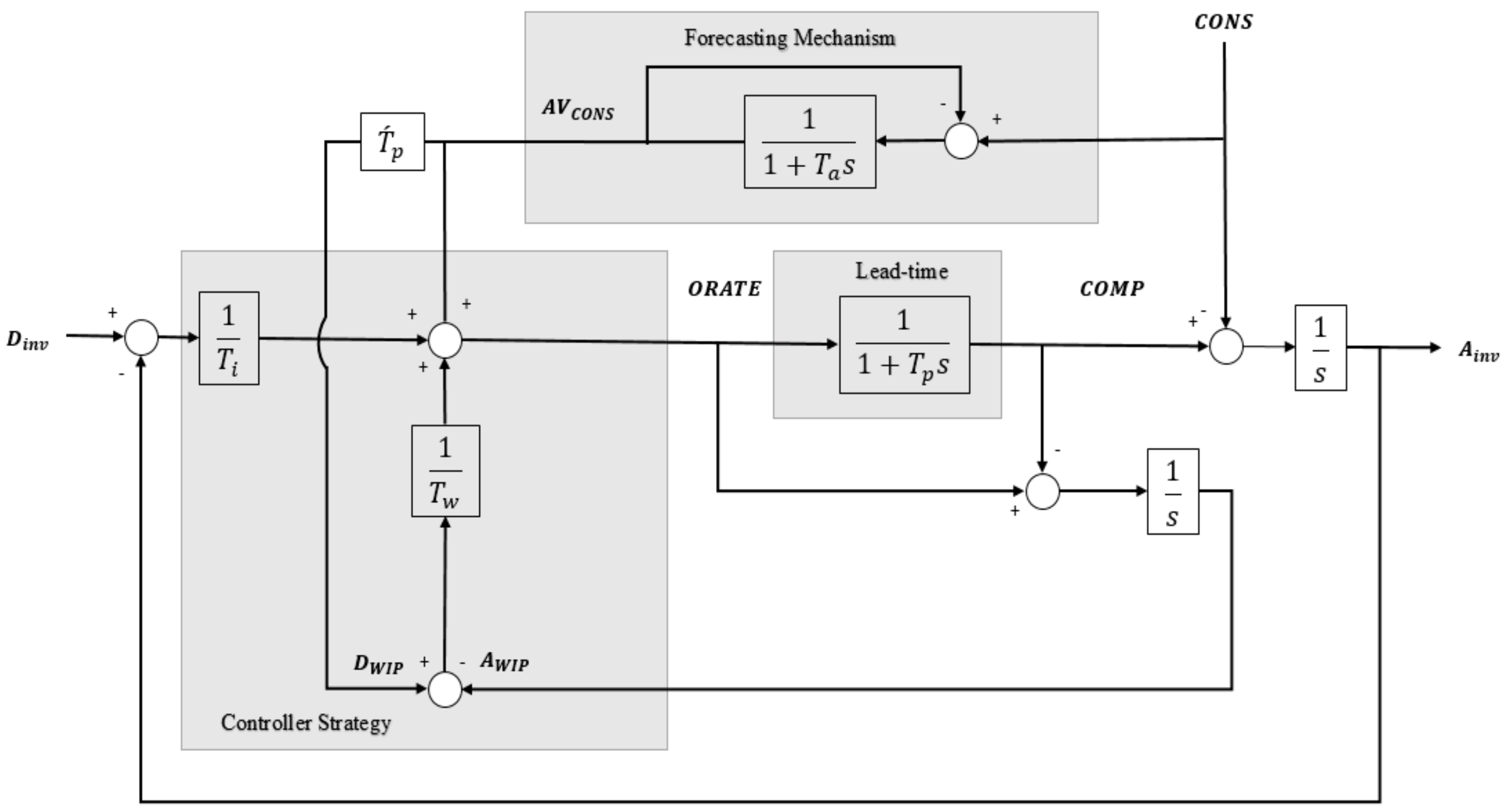
A production–inventory system is a basic unit in supply chain that integrates inventory control policies with the production process. In modelling and simulation practices, a production–inventory system is represented by a block diagram, the example of the well-known APIOPBCS being shown in Figure 1. There are three major parts in APIOPBCS, the forecasting mechanism, the production lead time, and the controller strategy [15,16,17,18,19,20,21,22].
- The forecasting mechanism is a feed-forward loop designed to provide the estimated average sales (AVCONS) and to set the desired work-in-process (WIP) level (DWIP). CONS represents the sales or consumptions. The feed forward gain () works as a safety factor to compensate the production delay and equals the production lead-time (Tp). The estimated average sales (AVCONS) is commonly used to control the inventory steady-state error. Exponential smoothing with time constant (Ta) representing the average age of the data is a forecasting method commonly used to smooth the demand because of its simplicity and comprehensibility in mathematics for practitioners. The DWIP is obtained from multiplying the AVCONS by feed forward gain .
- The production lead time represents the total time required between placing an order and receiving the product as a finished item in the inventory. The controller designer cannot manipulate the lead time as it is considered as a characteristic of the system. The production lead time in the production–inventory control system is modelled as a first order lag with time constant Tp that responds to a sudden change in the demand.
- The controller strategy utilizes the forward and feedback information to generate a sophisticated decision to determine the manufacturing rate for the production–inventory system. In the APIOBPCS model, a production policy based on the pipeline output where the completion rate (COMRATE) is compared to the averaged demand AVCONS and their difference is fed back to the controller. Ti is an inventory order constant time for proportional control.
The APIOBPCS model utilizes three policies (demand, inventory level, pipeline policies) to determine the Order Rate (ORATE). The average consumption rate AVCONS based on exponential smoothing forecasts with time constant Ta is the forward control policy. The feedback consists of two control polices, the fraction 1/Ti of the difference between the desired inventory Dinv and the actual inventory Ainv and the fraction 1/TW of the difference between the desired WIP DWIP and the actual WIP AWIP.
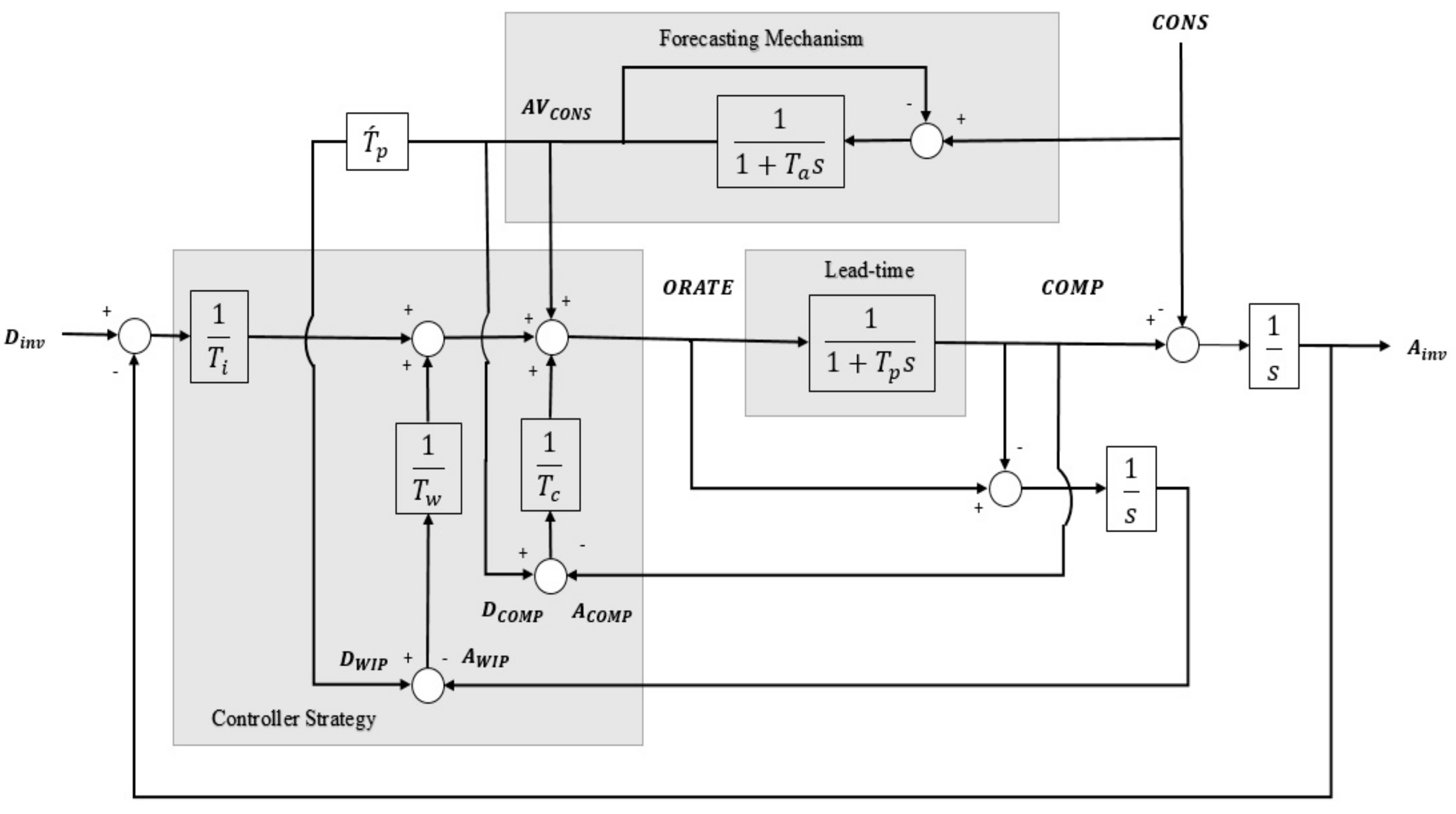
The 2APIOBPCS model [21] shown in Figure 2 has the similar structure to the APIOBPCS model, with an additional feedback loop using the fraction 1/Tc of the difference between the desired completion production rates DCOMP and the actual completion production rates ACOMP as an extra control for the production–inventory system. Tc is a constant time for the completion rate (COMP) for proportional control.
2.2. Mathematical Formulation of the Two APIOPBCS Models in the State Space
The state-space representation of the APIOBPCS model has three state variables [13,15,20,21,22]:
where x1 denotes the inventory level; x2 is the items in the production process that are not finished yet (WIP); x3 represents the consumption or sales state. The derivative state of the APIOBPCS model is:
The outputs of the system are represented by the inventory level Ainv and the order rate ORATE defined by
The continuous closed-loop state space representation of the APIOBPCS model is
Similarly, by considering the completion rates, the continuous closed-loop state space representation of the 2APIOBPCS model is expressed as [21]
2.3. Performance Metrics
The performance metrics that are used to evaluate the performance of production–inventory systems should have implications on total costs (inventory related costs and productions related costs) and customer service level (CSL) [23]. In this study, the dynamic performance of the production–inventory system is evaluated by firstly the variance ratio (Var) between the order rate and the consumption or the sales defined in Equation (12).
where refers to variance of the orders placed to the manufacturer and represents the consumption variance. The Var index is used as a metric to measure bullwhip effect. In this criterion, there is zero bullwhip if Var = 1; the system is amplified if Var > 1; the system is smoothed if Var < 1.
The second measure to evaluate inventory responsiveness of a production–inventory system is the integral of absolute error (IAE) between the actual and the target levels of inventory defined in Equation (13).
where t is the period and E refers to the error in the inventory levels measured as the deviation of the Ainv level from the Dinv level. The IAE measures positive and negative errors equally. A lower IAE indicates that the system has a better customer service level (CSL). The bullwhip effect and inventory responsiveness are two objectives that have direct impacts on the nature of the basic trade-offs between maintaining the order rates at the optimal performance, in order to avoid the impact of high amplification of orders, and maintaining stocks at a desired level to improve CSL.
3. Simulation Procedure and Experimental Considerations
3.1. Simulation Procedure
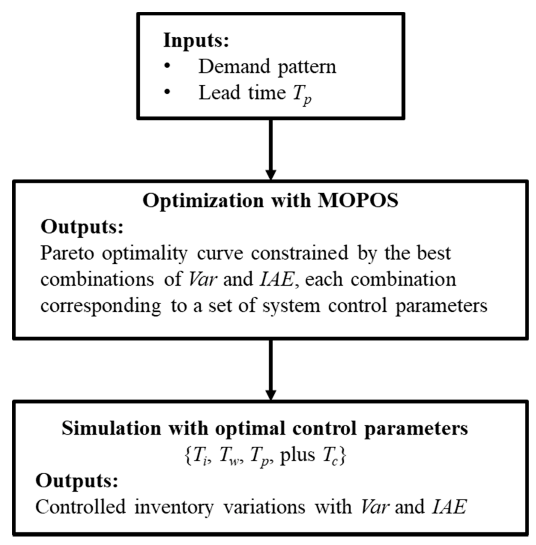
Simulations of a production–inventory system used to be conducted using some sets of input parameters mainly based on the practitioner’s experience in operating similar systems. The best values for the control parameters among the different sets of simulation outcomes are then determined by comparing the statistical results of these outcomes. The inputs must of course be reset for simulating a new system. By introducing a designated MOPSO algorithm into simulation using the APIOBPCS model [22], once feeding the demand pattern and production lead time to the system, the automatic simulation process can produce a set of control parameters (Ti, Tw and Ta), in which each set can achieve the best balance between the variance ratio (Var) and the integral of absolute error (IAE), in other words, between the bullwhip effect (cost-effectiveness for the industry) and CSL or customer satisfaction. These sets of control parameters are usually presented as a Pareto optimality curve, in which the system manager can choose any desired set on the curve as the best control parameters.
By embedding the designated MOPSO algorithm into the simulation, the process of dynamic simulation of a production–inventory system can be summarized in Figure 3. The inputs to the simulation are the demand pattern and the lead time required for orders. The inputs trigger the MOPSO algorithm for optimization constrained by both Var and IAE. The outputs of this optimization process are the best choices for the system configuration that can produce the optimal performance in terms of improving the system responsiveness related to CSL and reducing the demand amplification related to the bullwhip effect. A chosen set of the best control parameters is then fed to the system to simulate the desired order rate ORATE and inventory level Ainv, which would help the manager to adjust the stock level near the optimal status.
3.2. Experimental Considerations
Any simulation is subject to some system constraints and operational assumptions. As the purpose of our simulation is to make a leveled comparison on the dynamic performance between the APIOBPCS model and the 2APIOBPCS model, we choose a simple production–inventory system comprising one retailer and one manufacturer for one product so as to examine the difference in the dynamic performance of the two control models. Sophisticated production–inventory systems logically can only make the difference larger.
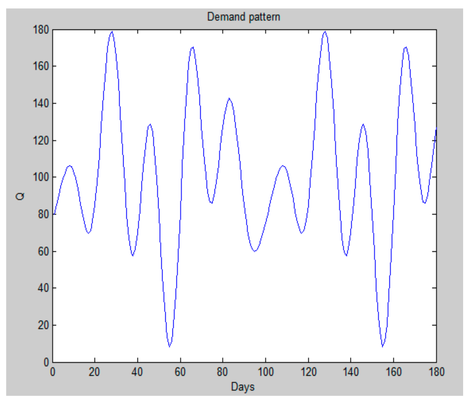
Since the demand pattern can vary largely, following the common practices in simulation of production–inventory systems, we choose a variable sinusoidal pattern as shown in Figure 4 to represent the random nature of demand to some extent. Other variables are assigned the values used in various published works in production–inventory simulations [8,13,14,17,18,19,24,25,26]. The major assumptions in all our simulations are as follows.
- The period of physical production lead time is four units of time (Tp = 4). Of course, this can be assigned to different values but it would not largely alter the general trend.
- Backorders (negative inventory) are permitted.
- The desired inventory is set to zero (Dinv = 0).
- Day is the basic time unit in the model.
- The simulation was run for 180 days for each scenario.
- The production process can only produce a single unit at a time.
The simulations with our designated MOPSO were conducted with MATLAB. The optimization process returns the best sets as a vector p1 = {Ta, Ti, Tw} for the APIOBPCS model. As the completion rate Tc for the 2APIOBPCS model is in practice a certain value not to be optimized, it is simply added to the vector p1 to form the control for the 2APIOBPCS model as p2 = {Ta, Ti, Tw, Tc}.
The parameters for MOPSO used in the simulation were:
- The maximum number of iterations was set to 100.
- The number of particles in the swarm was set to 50.
- The learning coefficients for local and global searches were both set to 2.
- The inertia weight was set as 0.6.
- The size of the archive was set to 20.
The performance of the two models was first examined by simulating them by the demand pattern under a normal scenario: Matched lead time with flexible production capacity, followed by three different scenarios: Matched lead time with fixed production capacity, mismatched lead time with flexible production capacity, and mismatched lead time with fixed production capacity. The implications of these scenarios are as follows.
- Matched lead time means that the actual lead time and the estimated lead time are assumed to be matched during the operation, or in other words, the ordered amount of product should be delivered by the manufacturer to the retailer on time.
- Mismatched lead time means that there is a delay of the ordered product from the manufacturer to the retailer. This may be caused by machine breakdowns and/or material shortages to the manufacturer. In such a situation, a longer lead time is expected. The mismatched scenarios evaluate the robustness of the two models by measuring how the systems can recover from such disruptions and get back to the normal level. Such a simulation is represented by a lead time starting at the nominal value Tp = 4, then to Tp = 6 for a period, and back to the normal Tp = 4.
- Flexible production capacity means that the manufacturer has no problem to produce the ordered product on time. Even if there is a disruption during production, the manufacturer is able to mitigate the negative impact without delaying the delivery of the ordered product.
- Fixed production capacity means that there is a limit for the manufacturer to produce the ordered product within the timeframe. In a normal scenario, the ordered amount would match the top limit of the manufacturer’s capacity. However, the situation is prone to any disruption to the production caused by machine breakdowns and/or material shortages. In such a situation, when the production capacity in a period is insufficient to complete the production for an order, the capacity of the next period is used to continue the production of this order. The order in the affected period is capped by a constant C, i.e.,
In our simulation, the capacity was set to C = 110 items per day (of course it can be a different number without losing generality).
4. Simulation Results and Discussion
The control vector p1 = {Ta, Ti, Tw} represents a Pareto curve of infinitely many combinations that can lead to optimal performance, and each combination can result in a set of simulation results. In this work, we selected three sets to simulate the two models separately (Table 1). These three selections correspond to three different ranges of the bullwhip effect as follows.
- Set 1: Bullwhip smoothing in range 0.8 < Var < 1
- Set 2: Bullwhip avoidance where Var = 1
- Set 3: Small bullwhip in range 1 < Var < 1.3
Note the optimal parameters for the simulation are resulted from MOPSO under the same demand pattern and lead time (Tp) that are the same for the two models in the same range of bullwhip effect simulated in this study. As a result, the values of the control parameters for the two models in the same range are the same. The completion rate for the 2APIOBPCS model is chosen in proportion to each set accordingly.
In our discussion on the simulation results, a new indicator named the ‘improved inventory responsiveness’ (IIR) is used, which is the percentage ratio of the IAE difference between the two models versus the IAE of the APIOBPCS model, i.e.,
4.1. Case 1: Matched Lead Time with Flexible Production Capacity
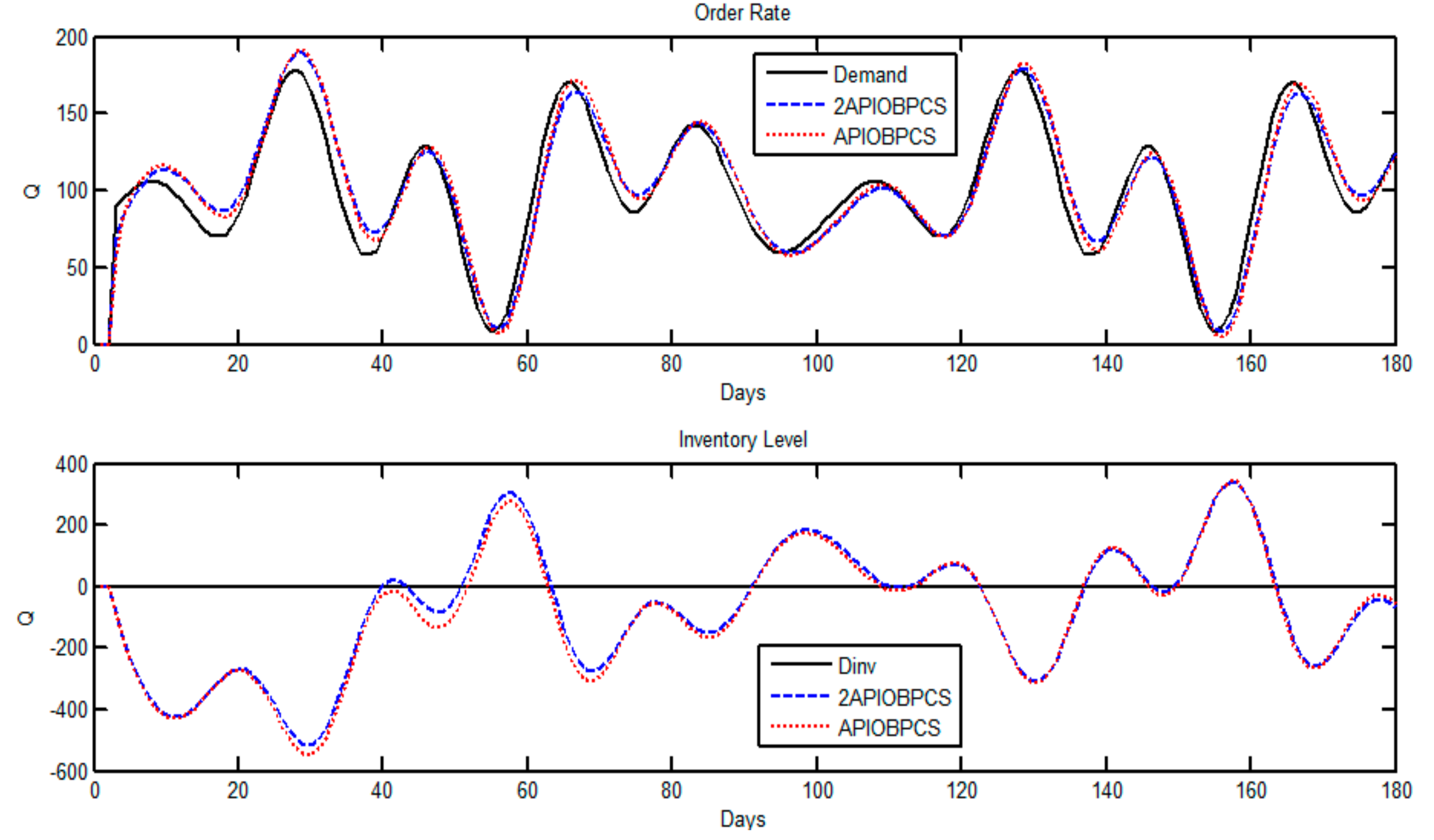
Table 2 shows the performances of the two models under the three optimal control sets for the system in this normal scenario. As expected, there is no difference in the bullwhip effect as the orders should be fulfilled with the same level for both models. However, with the information of partly completed order as the dynamic feedback, the system with the 2APIOBPCS model can produce a better IIR compared to the APIOBPCS model. The improvement varies from 3% for no and smoothed bullwhip effect to 9% for a small bullwhip effect. The improvement is the accumulated outcome over the period of simulation when on most occasions the inventory level of the 2APIOBPCS model is closer to the desired inventory level of zero compared to that of the APIOBPCS model as shown in Figure 5, even though the order rates of the two models are almost identical to each other during the period.
4.2. Case 2: Matched Lead Time with Fixed Production Capacity
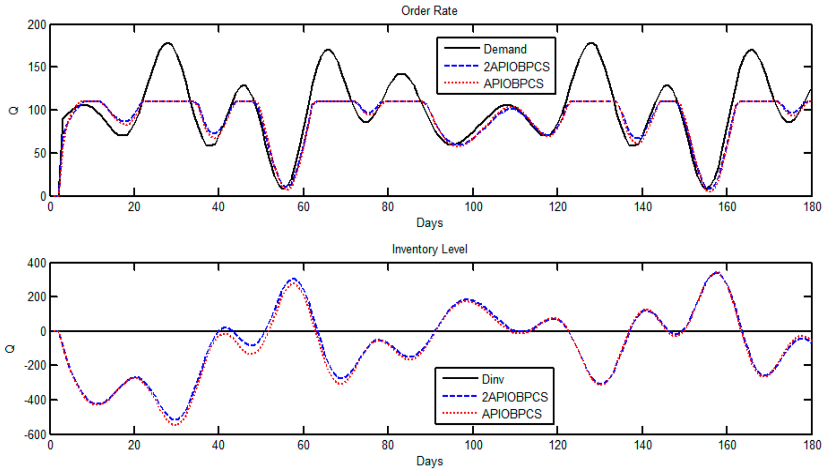
Table 3 shows the performances of the two models under the three optimal control sets for the system in this scenario. Due to the limit on the production capacity, a delay in product delivery is highly likely regardless of the level of orders. Owing to the uncertainties in product production and delivery, by introducing the capacity constraint (Figure 6), the estimated order was capped at the top limit, which effectively smoothed the bullwhip effect for both models, reflected in both models by a smaller Var. As the system waits for the slow production, the actual IAE is the same to the normal scenario in Case 1. This is in line with the observation reported in [18].
4.3. Case 3: Mismatched Lead Time with Flexible Production Capacity
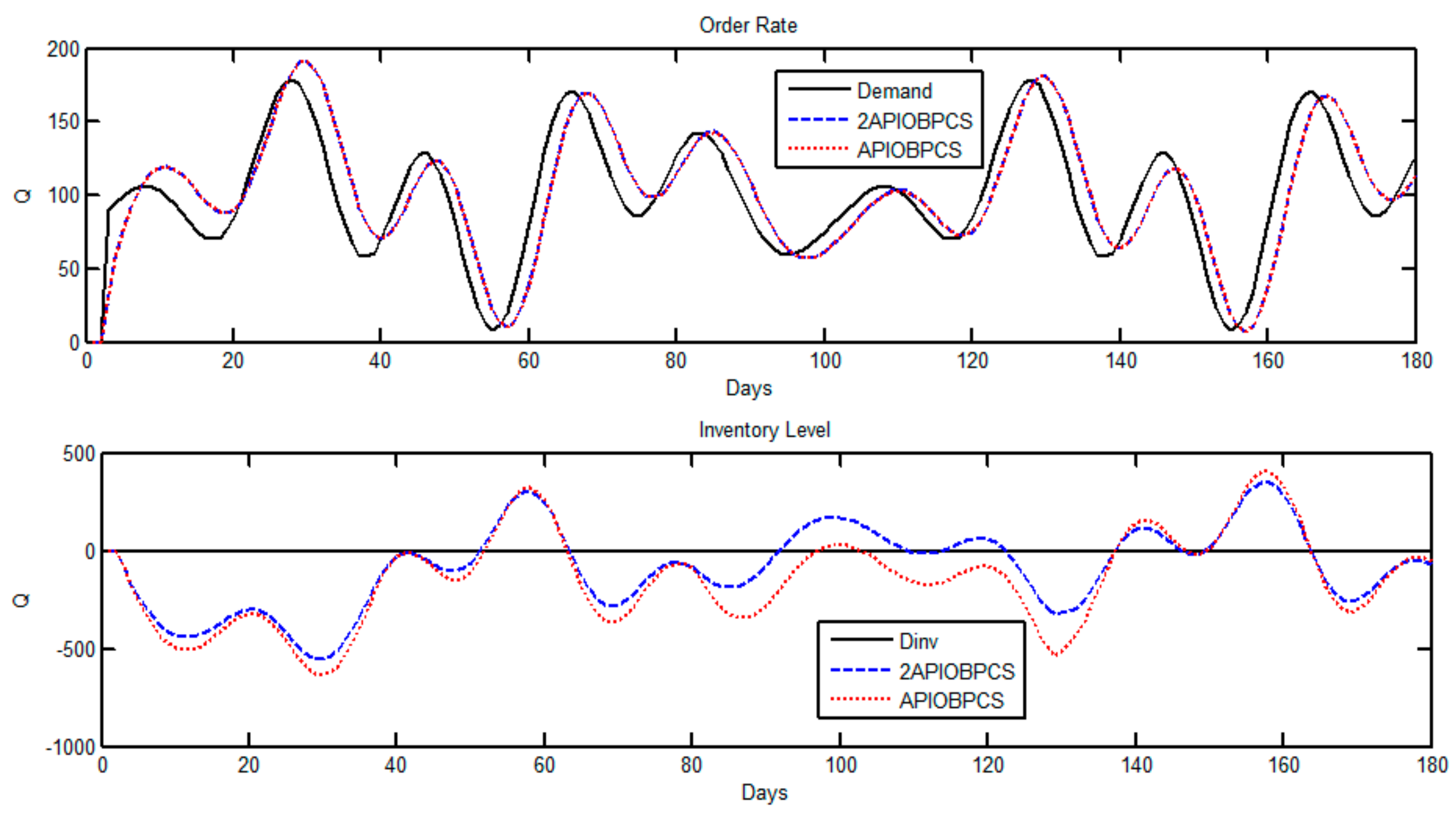
Table 4 shows the performances of the two models under the three optimal control sets for the system in this scenario. As the production capacity is sufficient to produce the ordered product, product delivery on time is guaranteed. In such a situation, the mismatched lead time between the order and delivery should be caused by miscalculation of the stock by the retailer or miscommunication between the retailer and the manufacturer. With the information of partly completed order as the dynamic feedback, the system with the 2APIOBPCS model in this case shows a significant advantage with a larger IIR compared to the APIOBPCS model. For example, if the retailer’s miscalculation resulted in a lower order than the required level, the 2APIOBPCS model can mitigate the potential loss with the dynamic feedback to reduce the IAE by 17% as if using the APIOBPCS model. If the retailer’s miscalculation resulted in a higher order than the required level, the 2APIOBPCS model can also mitigate the potential loss by reducing the IAE for 12% as if using the APIOBPCS model. For the desired situation without bullwhip effect, the IAE is reduced by about 14%. This accumulated outcome over the period of simulation is shown in Figure 7.
4.4. Case 4: Mismatched Lead Time with Fixed Production Capacity
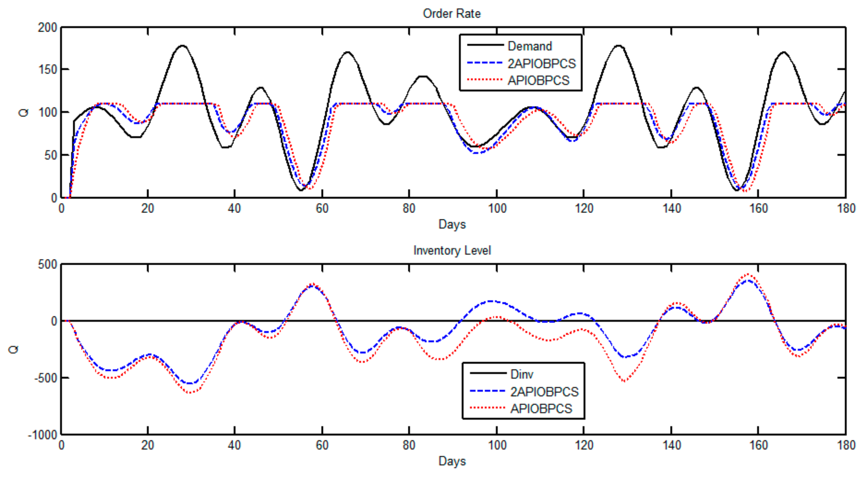
Table 5 shows the performances of the two models under the three optimal control sets for the system in this scenario. Similar to Case 2, due to the capacity constraint, a delay in product delivery is highly likely regardless of the level of orders or miscommunication between the retailer and the manufacturer (Figure 8). The capacity constraint on production effectively smoothed the bullwhip effect, which is reflected in both models by a smaller Var. As the system waits for the slow production, the actual IAE is the same to Case 3.
5. Conclusions
Modelling production–inventory system is a problem of multivariable input and multivariant output in mathematics. Hence, selecting the best system control parameters is a crucial managerial decision to achieve and dynamically maintain an optimal performance in terms of balancing the order rate and stock level under dynamic influence of many factors affecting the system operations. Simulation is perhaps the best means to deal with the dynamicity of such a system with multivariable input and multivariant output. By integrating our designated multi-objective particle swarm optimization (MOPSO) algorithm into the popular control model APIOBPCS and our newly modified model 2APIOBPCS for the production–inventory systems, this study compared the dynamic performances of these two models for modelling the production–inventory systems subjected to a random customer demand and production variations. By using the MOPSO optimized control parameters, our simulations point to the following trends between the two models:
- Both models can produce the situational best possible balance between the order rate and inventory level under the same bullwhip effort if the production lead time is matched, regardless of the production capacity. However, the 2APIOBPCS model seemed able to improve the inventory responsiveness by a few percentages compared to the APIOBPCS model.
- The 2APIOBPCS model seemed able to improve the inventory responsiveness by more than 10% compared to the APIOBPCS model under the same bullwhip effect if the production lead time is mismatched.
- By imposing a constraint to the production capacity, the bullwhip effect for both models seemed reduced but the inventory responsiveness kept the same.
The dynamic performance of the 2APIOBPCS model seemed better or no worse than that of the APIOBPCS model under different conditions. It looks more robust than the APIOBPCS model when the production lead time is miscalculated. Hence, the 2APIOPBCS model may have a good potential for companies to better manage their production–inventory systems to maintain optimal performance dynamically. However, we only regard our findings as some general trends in achieving optimal performance for production–inventory systems as these findings must be further cross-validated using different sophisticated cases for intensive simulation experiments by other researchers for objectiveness in the future.
Author Contributions
Conceptualization, H.A.-K. and W.G.; methodology, H.A.-K. and W.G.; software, H.A.-K.; validation, W.G.; formal analysis, H.A.-K. and W.G.; investigation, H.A.-K.; resources, C.C. and W.G.; data curation, H.A.-K.; writing—original draft preparation, H.A.-K.; writing—review and editing, W.G.; supervision, C.C. and W.G.; project administration, C.C. All authors have read and agreed to the published version of the manuscript.
Funding
This research received no external funding.
Institutional Review Board Statement
Not applicable.
Informed Consent Statement
Not applicable.
Conflicts of Interest
The authors declare no conflict of interest.
References
- Wikner, J.; Naim, M.M.; Spiegler, V.L.; Lin, J. IOBPCS based models and decoupling thinking. Int. J. Prod. Econ. 2017, 194, 153–166. [Google Scholar] [CrossRef]
- Zohourian, M. Supply Chain Decision Making under Demand Uncertainty and the Use of Control Systems: A Correlational Study. Ph.D. Thesis, Northcentral University, Scottsdale, AZ, USA, 2015. [Google Scholar]
- Negahban, A.; Smith, J.S. The effect of supply and demand uncertainties on the optimal production and sales plans for new products. Int. J. Prod. Res. 2016, 54, 3852–3869. [Google Scholar] [CrossRef]
- Dejonckheere, J.; Disney, S.M.; Lambrecht, M.R.; Towill, D.R. Measuring and avoiding the bullwhip effect: A control theoretic approach. Eur. J. Oper. Res. 2003, 147, 567–590. [Google Scholar] [CrossRef]
- Holweg, M.; Disney, S.; Holmström, J.; Småros, J. Supply chain collaboration: Making sense of the strategy continuum. Eur. Manag. J. 2005, 23, 170–181. [Google Scholar] [CrossRef]
- Disney, S.M.; Towill, D.R. Eliminating drift in inventory and order based production control systems. Int. J. Prod. Econ. 2005, 93, 331–344. [Google Scholar] [CrossRef]
- Mula, J.; Poler, R.; García-Sabater, J.P.; Lario, F.C. Models for production planning under uncertainty: A review. Int. J. Prod. Econ. 2006, 103, 271–285. [Google Scholar] [CrossRef] [Green Version]
- Sarimveis, H.; Patrinos, P.; Tarantilis, C.D.; Kiranoudis, C.T. Dynamic modeling and control of supply chain systems: A review. Comp. Oper. Res. 2008, 35, 3530–3561. [Google Scholar] [CrossRef]
- Vassian, H.J. Application of discrete variable servo theory to inventory control. J. Oper. Res. Soc. Am. 1955, 3, 272–282. [Google Scholar] [CrossRef]
- Lin, P.H.; Wong, D.S.H.; Jang, S.S.; Shieh, S.S.; Chu, J.Z. Controller design and reduction of bullwhip for a model supply chain system using z-transform analysis. J. Process. Control 2004, 14, 487–499. [Google Scholar] [CrossRef]
- Ortega, M.; Lin, L. Control theory applications to the production–inventory problem: A review. Int. J. Prod. Res. 2004, 42, 2303–2322. [Google Scholar] [CrossRef]
- Orzechowska, J.; Bartoszewicz, A.; Burnham, K.J.; Petrovic, D. Control theory applications in logistics–MPC and other approaches. Logistyka 2012, 12, 1769–1774. [Google Scholar]
- Towill, D.R. Dynamic analysis of an inventory and order based production control system. Int. J. Prod. Res. 1982, 20, 671–687. [Google Scholar] [CrossRef]
- John, S.; Naim, M.M.; Towill, D.R. Dynamic analysis of a WIP compensated decision support system. Int. J. Manuf. Syst. Des. 1994, 1, 283–297. [Google Scholar]
- Lin, J.; Naim, M.M.; Purvis, L.; Gosling, J. The extension and exploitation of the inventory and order based production control system archetype from 1982 to 2015. Int. J. Prod. Econ. 2017, 194, 135–152. [Google Scholar] [CrossRef]
- Mason-Jones, R.; Naim, M.M.; Towill, D.R. The impact of pipeline control on supply chain dynamics. Int. J. Logist. Manag. 1997, 8, 47–62. [Google Scholar] [CrossRef]
- Aggelogiannaki, E.; Sarimveis, H. Design of a novel adaptive inventory control system based on the online identification of lead time. Int. J. Prod. Econ. 2008, 114, 781–792. [Google Scholar] [CrossRef]
- Cannella, S.; Ciancimino, E. The APIOBPCS Deziel and Eilon parameter configuration in supply chain under progressive information sharing strategies. In Proceedings of the 2008 Winter Simulation Conference, WSC 2008, Miami, FL, USA, 7–10 December 2008; IEEE: Piscataway, NJ, USA, 2008; pp. 2682–2690. [Google Scholar]
- Tosetti, S.; Patino, D.; Capraro, F.; Gambier, A. Control of a production-inventory system using a PID controller and demand prediction. IFAC Proc. 2008, 41, 1869–1874. [Google Scholar] [CrossRef] [Green Version]
- AL-Khazraji, H.; Cole, C.; Guo, W. Dynamics analysis of a production-inventory control system with two pipelines feedback. Kybernetes 2017, 46, 1632–1653. [Google Scholar] [CrossRef]
- AL-Khazraji, H.; Cole, C.; Guo, W. Analysing the impact of different classical controller strategies on the dynamics performance of production-inventory systems using state space approach. J. Model. Manag. 2018, 13, 211–235. [Google Scholar] [CrossRef]
- AL-Khazraji, H.; Cole, C.; Guo, W. Multi-objective particle swarm optimisation approach for production-inventory control systems. J. Model. Manag. 2018, 13, 1037–1056. [Google Scholar] [CrossRef]
- Neely, A.; Richards, H.; Mills, J.; Platts, K.; Bourne, M. Designing performance measures: A structured approach. Int. J. Oper. Prod. Manag. 1997, 17, 1131–1152. [Google Scholar] [CrossRef]
- Jamalnia, A.; Feili, A. A simulation testing and analysis of aggregate production planning strategies. Prod. Plan. Control 2013, 24, 423–448. [Google Scholar] [CrossRef]
- Cannella, S.; González-Ramírez, R.G.; Dominguez, R.; López-Campos, M.A.; Miranda, P.A. Modelling and Simulation in Operations and Complex Supply Chains. Math. Probl. Eng. 2017, 2017, 8062958. [Google Scholar] [CrossRef] [Green Version]
- Zhou, L.; Naim, M.M.; Tang, O.; Towill, D.R. Dynamic performance of a hybrid inventory system with a Kanban policy in remanufacturing process. Omega 2006, 34, 585–598. [Google Scholar] [CrossRef]
Figure 1.
Block diagram of the automatic pipeline, inventory, and order based production control system (APIOBPCS) model.
Figure 1.
Block diagram of the automatic pipeline, inventory, and order based production control system (APIOBPCS) model.

Figure 2.
Block diagram of the 2APIOBPCS model.

Figure 3.
The process of dynamic simulation of a production–inventory system.

Figure 4.
The demand pattern for simulations.

Figure 5.
Simulation of Case 1 using Set 2 for the APIOBPCS and 2APIOBPCS models. Order rate (top) and inventory level (bottom).
Figure 5.
Simulation of Case 1 using Set 2 for the APIOBPCS and 2APIOBPCS models. Order rate (top) and inventory level (bottom).

Figure 6.
Simulation of Case 2 using Set 2 for the APIOBPCS and 2APIOBPCS models. Order rate (top) and inventory level (bottom).
Figure 6.
Simulation of Case 2 using Set 2 for the APIOBPCS and 2APIOBPCS models. Order rate (top) and inventory level (bottom).

Figure 7.
Simulation of Case 3 using Set 2 for the APIOBPCS and 2APIOBPCS models. Order rate (top) and inventory level (bottom).
Figure 7.
Simulation of Case 3 using Set 2 for the APIOBPCS and 2APIOBPCS models. Order rate (top) and inventory level (bottom).

Figure 8.
Simulation of Case 4 using Set 2 for the APIOBPCS and 2APIOBPCS models. Order rate (top) and inventory level (bottom).
Figure 8.
Simulation of Case 4 using Set 2 for the APIOBPCS and 2APIOBPCS models. Order rate (top) and inventory level (bottom).


Table 1.
Three optimal control sets to simulate the systems (Tc for 2APIOBPCS only).
| Set | Var | Ti | Tw | Ta | Tc |
|---|---|---|---|---|---|
| Set 1 | 0.8–1.0 | 3.91 | 0.55 | 6.71 | 10 |
| Set 2 | 1.0 | 5 | 1.13 | 5.66 | 21.9 |
| Set 3 | 1.0–1.3 | 3.5 | 1.2 | 6 | 2 |
Table 2.
Performances of Case 1 (the normal scenario) for the two models.
| Matched Lead Time with Fixed Production Capacity | |||||
|---|---|---|---|---|---|
| APIOBPCS | 2APIOBPCS | ||||
| Var | IAE | Var | IAE | IIR | |
| 0.85 | 3.57 × 10⁴ | 0.85 | 3.46 × 10⁴ | 3% | |
| 1.0 | 3.07 × 10⁴ | 1.0 | 2.97 × 10⁴ | 3% | |
| 1.25 | 2.84 × 10⁴ | 1.25 | 2.59 × 10⁴ | 9% | |
Table 3.
Performances of Case 2 for the two models.
| Matched Lead Time with Fixed Production Capacity | ||||
|---|---|---|---|---|
| APIOBPCS | 2APIOBPCS | |||
| Var | IAE | Var | IAE | IIR |
| 0.38 | 3.57 × 10⁴ | 0.38 | 3.46 × 10⁴ | 3% |
| 0.47 | 3.07 × 10⁴ | 0.45 | 2.97 × 10⁴ | 3% |
| 0.54 | 2.84 × 10⁴ | 0.54 | 2.59 × 10⁴ | 9% |
Table 4.
Performances of Case 3 for the two models.
| Mismatched Lead Time with Flexible Production Capacity | ||||
|---|---|---|---|---|
| APIOBPCS | 2APIOBPCS | |||
| Var | IAE | Var | IAE | IIR |
| 0.85 | 7.60 × 10⁴ | 0.85 | 6.32 × 10⁴ | 17% |
| 1 | 5.56 × 10⁴ | 1 | 4.76 × 10⁴ | 14% |
| 1.23 | 4.44 × 10⁴ | 1.23 | 3.93 × 10⁴ | 12% |
Table 5.
Performances of Case 4 for the two models.
| Mismatched Lead Time with Fixed Production Capacity | ||||
|---|---|---|---|---|
| APIOBPCS | 2APIOBPCS | |||
| Var | IAE | Var | IAE | IIR |
| 0.38 | 7.60 × 10⁴ | 0.38 | 6.32 × 10⁴ | 17% |
| 0.47 | 5.56 × 10⁴ | 0.45 | 4.76 × 10⁴ | 14% |
| 0.54 | 4.44 × 10⁴ | 0.54 | 3.93 × 10⁴ | 12% |
Publisher’s Note: MDPI stays neutral with regard to jurisdictional claims in published maps and institutional affiliations. |
© 2021 by the authors. Licensee MDPI, Basel, Switzerland. This article is an open access article distributed under the terms and conditions of the Creative Commons Attribution (CC BY) license (http://creativecommons.org/licenses/by/4.0/).
Share and Cite
MDPI and ACS Style
AL-Khazraji, H.; Cole, C.; Guo, W. Optimization and Simulation of Dynamic Performance of Production–Inventory Systems with Multivariable Controls. Mathematics 2021, 9, 568. https://0-doi-org.brum.beds.ac.uk/10.3390/math9050568
AMA Style
AL-Khazraji H, Cole C, Guo W. Optimization and Simulation of Dynamic Performance of Production–Inventory Systems with Multivariable Controls. Mathematics. 2021; 9(5):568. https://0-doi-org.brum.beds.ac.uk/10.3390/math9050568
Chicago/Turabian StyleAL-Khazraji, Huthaifa, Colin Cole, and William Guo. 2021. "Optimization and Simulation of Dynamic Performance of Production–Inventory Systems with Multivariable Controls" Mathematics 9, no. 5: 568. https://0-doi-org.brum.beds.ac.uk/10.3390/math9050568
Note that from the first issue of 2016, this journal uses article numbers instead of page numbers. See further details here.