An Extended SEIR Model with Vaccination for Forecasting the COVID-19 Pandemic in Saudi Arabia Using an Ensemble Kalman Filter

Abstract

In this paper, an extended SEIR model with a vaccination compartment is proposed to simulate the novel coronavirus disease (COVID-19) spread in Saudi Arabia. The model considers seven stages of infection: susceptible (S), exposed (E), infectious (I), quarantined (Q), recovered (R), deaths (D), and vaccinated (V). Initially, a mathematical analysis is carried out to illustrate the non-negativity, boundedness, epidemic equilibrium, existence, and uniqueness of the endemic equilibrium, and the basic reproduction number of the proposed model. Such numerical models can be, however, subject to various sources of uncertainties, due to an imperfect description of the biological processes governing the disease spread, which may strongly limit their forecasting skills. A data assimilation method, mainly, the ensemble Kalman filter (EnKF), is then used to constrain the model outputs and its parameters with available data. We conduct joint state-parameters estimation experiments assimilating daily data into the proposed model using the EnKF in order to enhance the model’s forecasting skills. Starting from the estimated set of model parameters, we then conduct short-term predictions in order to assess the predicability range of the model. We apply the proposed assimilation system on real data sets from Saudi Arabia. The numerical results demonstrate the capability of the proposed model in achieving accurate prediction of the epidemic development up to two-week time scales. Finally, we investigate the effect of vaccination on the spread of the pandemic.

1. Introduction

The novel coronavirus disease (COVID-19) first appeared in Wuhan city, and due to its high transmission rate, the virus has been rapidly spreading all over the world. On 8 March 2020, the WHO announced COVID-19 as a global pandemic [1]. As of 1 January 2021, there are over 100 million reported cases, and a death toll exceeding 2 million.

In the absence of a ready-to-use vaccine, and besides medical and biological research, mathematical models can play an important role in understanding and predicting disease transmission. Moreover, it helps to implement appropriate measures and efficient strategies to control the pandemic’s spread and mitigate its impact.

Mathematical epidemic models based on the SIR model [2] are widely used to study the spread of a disease in a population [3,4,5,6,7]. Recently, several mathematical models have been developed to study the transmission dynamics of COVID-19 [8,9,10,11]. However, these models suffer from various sources of uncertainties, due to the incomplete description of the biological processes governing the disease spread, and also due to some involved parameters being poorly known. One way to mitigate these uncertainties is to constrain epidemic forecasting models with available data. These data can be combined with the model output to improve its prediction and reduce uncertainties [12,13,14]. This process, known as data assimilation, sequentially adjusts the model state and parameters once data become available to keep the model as close as possible to the real track [15].

The ensemble Kalman filter (EnKF) is a popular data assimilation technique introduced by [16] to tackle large-scale, sequential, and non-linear problems. The EnKF is a Monte Carlo implementation of the traditional Kalman filter [17], operating in cycles of two steps: (i) A forecast step in which a set of state samples, or ensemble members, are integrated forward in time with the model, and (ii) an analysis step to update the forecasted members with available data based on the Bayes rule in a Gaussian framework [15,16]. Because of its affordable computational cost, robust performance, nonintrusive formulation, and ease of implementation, the EnKF have been successfully implemented in many geophysical applications, including weather forecasting [18,19,20], hydrology and reservoir applications [21,22,23,24,25,26], ocean modeling [27,28,29,30,31], and flood modeling [32,33,34].

In epidemiology, previous studies have used data assimilation in the context of both variational and Kalman filter methods [35,36,37,38]. The Reference [39] used the EnKF to estimate the parameters of a stochastic SEIR model. The Reference [40] applied a deterministic variant of the EnKF, the Ensemble Adjustment Kalman Filter (EAKF), in combination with a network of SEIR models, simulating different connected cities. The Reference [41] used an ensemble smoother with a multiple data assimilation (ESMDA) approach for parameter estimation in a SEIR model. The Reference [42] also implemented the ESMDA to effectively estimate the parameters of a more sophisticated SEIR model accounting for age-classes and compartments of the sick, hospitalized, and dead. The Reference [43] used an EnKF approach for parameter estimation and shot-term forecasts with a simple SIR model. The Reference [44] proposed an EnKF for estimating unmeasurable state variables and unknown parameters of a SIRV model, which takes into account the circulation of free coronavirus in the environment. In the context of variational data assimilation methods, the Reference [45] performed parameter estimation and predictions using a SIR model, while [46] proposed a modified SEIR model that distinguishes between symptomatic and asymptomatic, and conducted observation sensitivity experiments to identify suitable observing strategies. However, these studies did not consider the impact of vaccination on the pandemic spread.

This work therefore aims to study the impact of vaccination on the COVID-19 spread. An extended SEIR model comprising of seven compartments—susceptible, exposed, infectious, quarantined, recovered, deaths, and vaccinated—is then proposed. First, we conduct a mathematical analysis to illustrate the non-negativity, boundedness, epidemic equilibrium, existence, and uniqueness of the endemic equilibrium, and the basic reproduction number of the model. A Joint-EnKF is implemented for state-parameters estimation by assimilating COVID-19 data into the model. By considering uncertainties in all model states and poorly known parameters, our ensemble data assimilation approach computes updates of both state and parameter ensembles. The estimated set of model state and parameters is then used to assess the model prediction skill. The proposed approach is validated with the cases reported from the most-infected Gulf country, Saudi Arabia, showing a great ability to provide accurate and consistent forecasts up to two weeks. We finally investigate the effect of vaccination on the spread of the pandemic, showing a notable decrease in the number of cases.

The remainder of this paper is organized as follows. Section 2 presents the extended SEIR model and briefly describes the Joint-EnKF algorithm. Section 3 is devoted to the mathematical analysis of the model. The numerical results are presented and discussed in Section 4. Section 5 concludes the study, with a summary of the main results.

2. Model and Assimilation Scheme

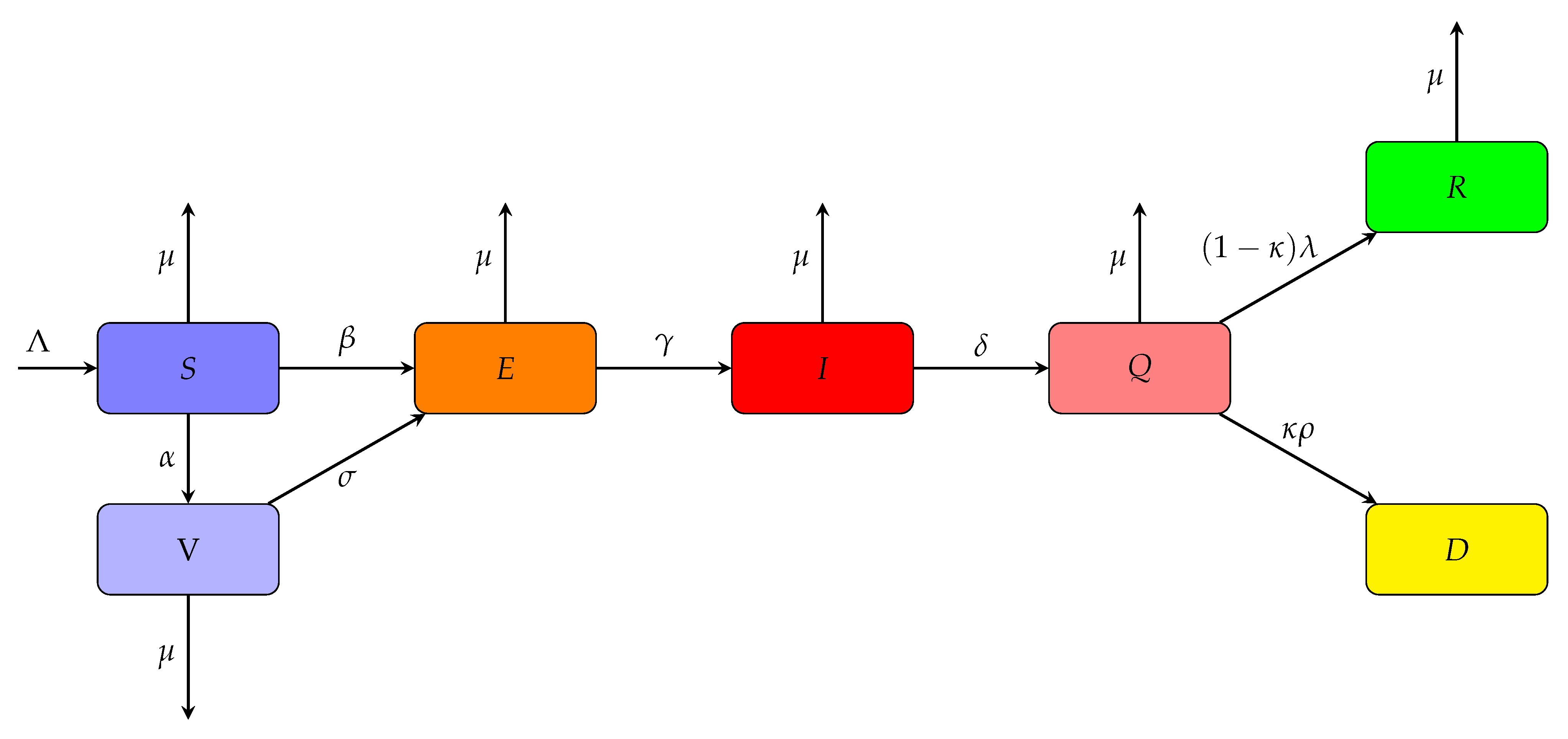
2.1. Extended SEIR Model

We extend the SEIR model to seven compartments to simulate the epidemic of COVID-19. Seven state variables are considered within a population, that is, $S\left(t\right)$, $E\left(t\right)$, $I\left(t\right)$, $Q\left(t\right)$, $R\left(t\right)$, $D\left(t\right)$, and $V\left(t\right)$, denoting the number of susceptible, exposed (infected, but not yet infectious), infectious (not yet quarantined), quarantined (confirmed and infected), recovered, dead, and vaccinated cases, respectively. The disease transmission flow of the proposed model is sketched in Figure 1. The model is then governed by the following set of nonlinear ordinary differential equations:

$$\begin{array}{cc}\hfill {\displaystyle \frac{dS\left(t\right)}{dt}}& =\Lambda -\beta S\left(t\right)I\left(t\right)-\alpha S\left(t\right)-\mu S\left(t\right),\hfill \\ \hfill {\displaystyle \frac{dE\left(t\right)}{dt}}& =\beta S\left(t\right)I\left(t\right)-\gamma E\left(t\right)+\sigma \beta V\left(t\right)I\left(t\right)-\mu E\left(t\right),\hfill \\ \hfill {\displaystyle \frac{dI\left(t\right)}{dt}}& =\gamma E\left(t\right)-\delta I\left(t\right)-\mu I\left(t\right),\hfill \\ \hfill {\displaystyle \frac{dQ\left(t\right)}{dt}}& =\delta I\left(t\right)-(1-\kappa )\lambda Q\left(t\right)-\kappa \rho Q\left(t\right)-\mu Q\left(t\right),\hfill \\ \hfill {\displaystyle \frac{dR\left(t\right)}{dt}}& =(1-\kappa )\lambda Q\left(t\right)-\mu R\left(t\right),\hfill \\ \hfill {\displaystyle \frac{dD\left(t\right)}{dt}}& =\kappa \rho Q\left(t\right),\hfill \\ \hfill {\displaystyle \frac{dV\left(t\right)}{dt}}& =\alpha S\left(t\right)-\sigma \beta V\left(t\right)I\left(t\right)-\mu V\left(t\right),\hfill \end{array}$$

(1)

with non-negative initial conditions $S\left(0\right)=S_0$, $E\left(0\right)=E_0$, $I\left(0\right)=I_0$, $Q\left(0\right)=Q_0$, $R\left(0\right)=R_0$, $D\left(0\right)=D_0$, and $V\left(0\right)=V_0$. The coefficients $\Lambda$, $\beta$, $\alpha$, $\mu$, $\gamma$, $\sigma$, $\delta$, $\kappa$, $\lambda$, and $\rho$ represent the new births and new residents per unit of time, transmission rate divided by N, vaccination rate (rate of people who are vaccinated), natural death rate, average latent time, average quarantine time, mortality rate, average days until recovery, and average days until death, respectively. $\sigma$ is the vaccine inefficacy $(0\le \sigma \le 1)$. So $1-\sigma$ represents the vaccine efficacy. If $\sigma =0$, the vaccine offers $100\%$ protection against the disease. $N=S+E+I+Q+R+D+V$ is the total population size. Finally, system (1) is solved using a fourth-order Runge–Kutta method.

2.2. Ensemble Kalman Filter (EnKF)

Consider the following nonlinear data assimilation problem:

$$\begin{array}{cc}\hfill {\mathbf{x}}_{k+1}& =\mathcal{M}\left({\mathbf{x}}_k,\theta \right)+{\eta }_{k+1},\hfill \\ \hfill {\mathbf{y}}_{k+1}& =\mathcal{H}\left({\mathbf{x}}_{k+1}\right)+{ϵ}_{k+1},\hfill \end{array}$$

(2)

where ${\mathbf{x}}_k$ is the state vector of the model at time $t_k$, $\mathcal{M}$ is the dynamical operator (system (1)) that integrates the model state from time $t_k$ to time $t_{k+1}$, $\theta$ is the parameters vector, ${\mathbf{y}}_{k+1}$ is the observation vector (active, recovered, and death cases) at time $t_{k+1}$, $\mathcal{H}$ is the observation operator that projects the state space onto the observation space, and ${\eta }_{k+1}$ and ${ϵ}_{k+1}$ are model and observation noises assumed to follow Gaussian distributions with zero mean and covariances ${\mathbf{Q}}_{k+1}$ and ${\mathbf{R}}_{k+1}$, respectively.

At every forecast step, we integrate the ensemble members with the dynamical model (1). The predicted state mean and the associated error covariance matrix are then estimated

$${\widehat{\mathbf{x}}}_{k+1}^f={\displaystyle \frac{1}{N_e}}\sum _{i=1}^{N_e}{\mathbf{x}}_{k+1}^{f,i},$$

(3)

$${\widehat{\mathbf{P}}}_{k+1}^f={\displaystyle \frac{1}{N_e-1}}\sum _{i=1}^{N_e}\left({\mathbf{x}}_{k+1}^{f,i}-{\widehat{\mathbf{x}}}_{k+1}^f\right){\left({\mathbf{x}}_{k+1}^{f,i}-{\widehat{\mathbf{x}}}_{k+1}^f\right)}^T={\mathbf{X}}_{k+1}^f{\left({\mathbf{X}}_{k+1}^f\right)}^T,$$

(4)

where $N_e$ is the number of ensemble members.

The Joint-EnKF consists of estimating the augmented state-parameters vector ${\mathbf{z}}_{k+1}=\left[{\mathbf{x}}_{k+1}^T,{\theta }^T\right]$ at each time $t_{k+1}$ given the observation ${\mathbf{y}}_{k+1}$. The prediction step of the Joint-EnKF becomes:

$${\mathbf{z}}_{k+1}^f=\tilde{\mathcal{M}}\left({\mathbf{z}}_k,\theta \right)+{\eta }_{k+1}=\left[\begin{array}{c}\mathcal{M}\left({\mathbf{x}}_k,\theta \right)+{\eta }_{k+1}\\ \theta \end{array}\right],$$

(5)

where $\tilde{\mathcal{M}}$ is the augmented nonlinear dynamic operator for the joint state-parameters. With similar computations as in (4), the joint state-parameters error covariance matrix for the augmented ensemble vectors ${\mathbf{z}}_{k+1}^{f,i}$ is given by

$${\widehat{\mathbf{P}}}_{k+1}^f=\left[\begin{array}{c}{\widehat{\mathbf{P}}}_{{\mathbf{x}}_{k+1}{\mathbf{x}}_{k+1}}^f{\widehat{\mathbf{P}}}_{{\mathbf{x}}_{k+1}{\theta }_{k+1}}^f\\ {\widehat{\mathbf{P}}}_{{\theta }_{k+1}{\mathbf{x}}_{k+1}}^f{\widehat{\mathbf{P}}}_{{\theta }_{k+1}{\theta }_{k+1}}^f\end{array}\right]=\left[\begin{array}{c}{\mathbf{X}}_{{\mathbf{x}}_{k+1}}^f{\left({\mathbf{X}}_{{\mathbf{x}}_{k+1}}^f\right)}^T{\mathbf{X}}_{{\mathbf{x}}_{k+1}}^f{\left({\mathbf{X}}_{{\theta }_{k+1}}^f\right)}^T\\ {\mathbf{X}}_{{\theta }_{k+1}}^f{\left({\mathbf{X}}_{{\mathbf{x}}_{k+1}}^f\right)}^T{\mathbf{X}}_{{\theta }_{k+1}}^f{\left({\mathbf{X}}_{{\theta }_{k+1}}^f\right)}^T\end{array}\right],$$

(6)

where ${\mathbf{X}}_{\theta }$ denotes the parameter ensemble perturbations. The updated joint state and parameters are then computed using the current observation ensemble ${\mathbf{y}}_{k+1}^i$:

$${\mathbf{z}}_{k+1}^{a,i}={\mathbf{z}}_{k+1}^{f,i}+{\widehat{\mathbf{P}}}_{k+1}^f{\tilde{\mathcal{H}}}^T{\left(\tilde{\mathcal{H}}{\widehat{\mathbf{P}}}_{k+1}^f{\tilde{\mathcal{H}}}^T+{\mathbf{R}}_{k+1}\right)}^{-1}\left[{\mathbf{y}}_{k+1}^i-\tilde{\mathcal{H}}{\mathbf{z}}_{k+1}^{f,i}\right],$$

(7)

where $\tilde{\mathcal{H}}=\left[\mathcal{H}\mathbf{0}\right]$ is the augmented observational operator with the zero matrix.

3. Mathematical Analysis of the COVID-19 Model

In this section, we discuss the boundedness, non-negativity, epidemic equilibrium, endemic equilibrium, and basic reproduction number of the COVID-19 model (1).

3.1. Non-Negativity of the Model

Theorem 1. 

If $S_0\ge 0$, $E_0\ge 0$, $I_0\ge 0$, $Q_0\ge 0$, $R_0\ge 0$, $D_0\ge 0$, and $V_0\ge 0$, then the solutions of system (1) remain non-negative for all $t>0$.

Proof of Theorem 1.

From the first equation of system (1), we have:

$${\displaystyle \frac{dS}{dt}}\ge -\mu S.$$

(8)

Integrating Equation (8), we get

$$S\left(t\right)\ge S_0{e}^{-\mu t}\ge 0.$$

(9)

Hence, $S\left(t\right)$ remains non-negative for all $t>0$. Similarly, using the remaining equations of system (1), we obtain $E\left(t\right)\ge 0$, $I\left(t\right)\ge 0$, $Q\left(t\right)\ge 0$, $R\left(t\right)\ge 0$, $D\left(t\right)\ge 0$, and $V\left(t\right)\ge 0$. Therefore, Theorem 1 is proved. □

3.2. Boundedness of the Model

Theorem 2. 

All solutions of the proposed model with non-negative initial conditions are bounded and $N\left(t\right)\le {\displaystyle \frac{\Lambda }{\mu }}$ for all $t>0$.

Proof of Theorem 2.

Adding all the equations in the system (1), the growth rate of the total population can be written as

$${\displaystyle \frac{dN}{dt}}={\displaystyle \frac{dS}{dt}}+{\displaystyle \frac{dE}{dt}}+{\displaystyle \frac{dI}{dt}}+{\displaystyle \frac{dQ}{dt}}+{\displaystyle \frac{dR}{dt}}+{\displaystyle \frac{dD}{dt}}+{\displaystyle \frac{dV}{dt}}.$$

(10)

From Equation (10), we have the following equation:

$${\displaystyle \frac{dN}{dt}}=\Lambda -\mu N.$$

(11)

Integrating both sides of Equation (11) gives the solution for $N\left(t\right)$ as follows

$$N\left(t\right)={\displaystyle \frac{\Lambda }{\mu }}+\left(N_0-{\displaystyle \frac{\Lambda }{\mu }}\right)e^{-\mu t}.$$

(12)

Thus, when $t\to \infty$, we find that

$$N\left(t\right)\le {\displaystyle \frac{\Lambda }{\mu }}.$$

(13)

Finally, Theorem 1 and Equation (13) give

$$0\le N\left(t\right)\le {\displaystyle \frac{\Lambda }{\mu }}.$$

(14)

Thus, $S\left(t\right)$, $E\left(t\right)$, $I\left(t\right)$, $Q\left(t\right)$, $R\left(t\right)$, $D\left(t\right)$, and $V\left(t\right)$ are bounded and Theorem 2 is proved. □

3.3. Epidemic Equilibrium and Basic Reproduction Number of the Model

The epidemic equilibrium $X^0$ of system (1) is obtained by setting all the derivatives to zero with $I=0$, that yields to:

$$X^0=\left({\displaystyle \frac{\Lambda }{\mu +\alpha }},0,0,0,0,0,{\displaystyle \frac{\alpha \Lambda }{\mu (\mu +\alpha )}}\right).$$

(15)

$R_0$ is computed using the next-generation matrix concept [47]. Let $X={(E,I)}^T$. System (1) can be written as

$$X^{\prime }=\mathbb{F}\left(X\right)-\mathbb{W}\left(X\right),$$

(16)

where $\mathbb{F}\left(X\right)={\left(\beta SI+\sigma \beta IV,0\right)}^T$ and $\mathbb{W}\left(X\right)={\left((\mu +\delta )E,-\gamma E+(\mu +\delta )\right)}^T$. Their corresponding Jacobian matrices at the disease-free equilibrium are

$$F=\left(\begin{array}{cc}0& \beta S^0+\sigma \beta V^0\\ 0& 0\end{array}\right),W=\left(\begin{array}{cc}\mu +\gamma & 0\\ -\gamma & \mu +\delta \end{array}\right).$$

(17)

According to [47], the basic reproduction number $R_0$ is the spectral radius of the next-generation matrix $F{W}^{-1}$. That gives

$$R_0={\displaystyle \frac{\beta \gamma }{\left(\mu +\gamma \right)\left(\mu +\delta \right)}}\left(S^0+\sigma V^0\right).$$

(18)

Substituting $S^0$ and $V^0$ from Equation (15) into Equation (20) yields the following formula for the basic reproduction number of system (1):

$$R_0={\displaystyle \frac{\beta \gamma \Lambda (\mu +\alpha \sigma )}{\mu \left(\mu +\gamma \right)\left(\mu +\delta \right)(\mu +\alpha )}},$$

(19)

used to measure the transmission potential of a disease. It is the number of secondary cases or new infections produced by a single infectious individual in a completely susceptible population [47,48]. An epidemic is expected to increase exponentially if $R_0>1$, and to end if $R_0<1$ [47].

Theorem 3. 

The disease-free equilibrium $X^0$ is locally asymptotically stable if $R_0<1$, and unstable if $R_0>1$.

Proof of Theorem 3.

System (1) can be written in a simplified form by eliminating the sixth equation for the death compartment (D). This is due to the fact that the state D only appears in the corresponding differential equation and has no significance on the overall system. The number of deaths can be determined from $D=N-S-E-I-Q-R-V$. The Jacobian matrix of the reduced model (1) at the disease-free equilibrium is given by

$$J\left(X^0\right)=\left(\begin{array}{cccccc}-{ϵ}_1& 0& -\beta S^0& 0& 0& 0\\ 0& -{ϵ}_2& \beta \left(S^0+\sigma V^0\right)& 0& 0& 0\\ 0& \gamma & -{ϵ}_3& 0& 0& 0\\ 0& 0& \delta & -{ϵ}_4& 0& 0\\ 0& 0& 0& \lambda \left(1-\kappa \right)& -\mu & 0\\ \alpha & 0& -\sigma \beta V^0& 0& 0& -\mu \end{array}\right),$$

(20)

where ${ϵ}_1=-(\alpha +\mu )$, ${ϵ}_2=-(\gamma +\mu )$, ${ϵ}_3=-(\delta +\mu )$, and ${ϵ}_4=-(\lambda (1-\kappa )+\kappa \rho +\mu )$. $J\left(X^0\right)$ has ${\lambda }_1=-{ϵ}_1<0$, ${\lambda }_2=-{ϵ}_4<0$, ${\lambda }_3={\lambda }_4=-\mu <0$. The remaining two eigenvalues are

$$\begin{array}{cc}\hfill {\lambda }_5& =-{\displaystyle \frac{1}{2}}\left({ϵ}_2+{ϵ}_3+\sqrt{{\left({ϵ}_2-{ϵ}_3\right)}^2+4{ϵ}_2{ϵ}_3{R}_0}\right),\hfill \\ \hfill {\lambda }_6& =-{\displaystyle \frac{1}{2}}\left({ϵ}_2+{ϵ}_3-\sqrt{{\left({ϵ}_2-{ϵ}_3\right)}^2+4{ϵ}_2{ϵ}_3{R}_0}\right).\hfill \end{array}$$

(21)

when $R_0<1$, we have ${\lambda }_5<0$ and ${\lambda }_6<0$. Since all the eigenvalues are negative, the disease-free equilibrium $X^0$ is locally asymptotically stable. If $R_0>1$, we have ${\lambda }_5<0$ and ${\lambda }_6>0$, and the disease-free equilibrium $X^0$ is locally asymptotically unstable [49]. □

3.4. Existence and Uniqueness of the Endemic Equilibrium

In this section, we investigate the existence and uniqueness of the endemic equilibrium when $R_0>1$. Let $X^{*}=(S^{*},E^{*},I^{*},Q^{*},D^{*},V^{*})$ be the endemic equilibrium of model (1). The endemic equilibrium is obtained by setting all the derivatives in model (1) to zero, giving

$$\begin{array}{c}\hfill \Lambda -\beta S^{*}{I}^{*}-\alpha S^{*}-\mu S^{*}=0,\\ \hfill \beta S^{*}{I}^{*}-\gamma E^{*}+\sigma \beta V^{*}{I}^{*}-\mu E^{*}=0,\\ \hfill \gamma E^{*}-\delta I^{*}-\mu I^{*}=0,\\ \hfill \delta I^{*}-(1-\kappa )\lambda Q^{*}-\kappa \rho Q^{*}-\mu Q^{*}=0,\\ \hfill (1-\kappa )\lambda Q^{*}-\mu R^{*}=0,\\ \hfill \alpha S^{*}-\sigma \beta V^{*}{I}^{*}-\mu V^{*}=0.\end{array}$$

(22)

Solving the first, third, and fifth equations of (22) in terms of $I^{*}$ gives

$$E^{*}={\displaystyle \frac{{ϵ}_3}{\gamma }}{I}^{*},Q^{*}={\displaystyle \frac{\delta }{{ϵ}_4}}{I}^{*},S^{*}={\displaystyle \frac{\Lambda }{\beta I^{*}+{ϵ}_1}},$$

(23)

where ${ϵ}_1=\mu +\alpha$, ${ϵ}_3=\mu +\delta$, and ${ϵ}_4=\mu +\lambda (1-\kappa )+\kappa \rho$. Adding the second and sixth equation in (22) gives

$$V^{*}={\displaystyle \frac{\Lambda \beta \gamma I+\Lambda \alpha \gamma -{ϵ}_2{ϵ}_3\left(\beta I+{ϵ}_1\right)I}{\mu \gamma \left(\beta I+{ϵ}_1\right)}}.$$

(24)

Now substituting the expressions of $S^{*}$, $E^{*}$, and $V^{*}$ in the second equation of (22), we get the following quadratic equation for $I^{*}$:

$$a_2{I^{*}}^2+a_1{I}^{*}+a_0=0,,$$

(25)

where

$$\begin{array}{c}\hfill a_0=\mu {ϵ}_1{ϵ}_2{ϵ}_3\left(1-R_0\right),\\ \hfill a_1={ϵ}_1{ϵ}_2{ϵ}_3+\mu \beta {ϵ}_2{ϵ}_3-\Lambda {\beta }^2\gamma \sigma ,\\ \hfill a_2=\beta {ϵ}_2{ϵ}_3.\end{array}$$

(26)

It is clear that $a_2$ is always positive and $a_0$ is negative when $R_0>1$. Therefore, there is a unique positive value for $I^{*}$, and consequently, a unique endemic equilibrium $X^{*}$ when $R_0>1$.

4. Results and Discussion

The proposed modeling system was applied to forecast the COVID-19 pandemic in Saudi Arabia. Data are available from the Saudi Center for Diseases Prevention and Control [50]. These include the number of deaths, as well as recovered and confirmed cases. The total number of deaths, active cases, and recovered cases were assimilated daily, and model parameters were also updated using the Joint-EnKF.

4.1. Assimilation Settings

In this section, we cover the period before the vaccine becomes available. Therefore, state and parameters related to vaccination are excluded from the model at this stage. The state vector x to be estimated is then composed of six elements

$$x=\left[SEIQRD\right],$$

(27)

and the parameters to be estimated become

$$\theta =\left[\Lambda \beta \mu \gamma \delta \kappa \lambda \rho \right].$$

(28)

The augmented state vector to be estimated is then:

$$z=\left[x^{T}log\left({\theta }^T\right)\right],$$

(29)

where the parameters are in a logarithmic sense in order to avoid negative values in the model.

We set the initial numbers of infected and exposed people to $I\left(0\right)=E\left(0\right)=3$, three times the number of accumulated positive tests $\left(Q_0=1\right)$ provided by March 2nd [50]. The initial numbers of recovered, and death cases are $R\left(0\right)=D\left(0\right)=0$. The total population and the total number of susceptible cases are $N\left(0\right)=$ 34,218,000 and $S\left(0\right)=N\left(0\right)-E\left(0\right)-I\left(0\right)-Q\left(0\right)-R\left(0\right)-D\left(0\right)$, respectively. We consider the following two periods: the first period concerns the period of the beginning of the pandemic when the intervention had not been applied using a basic reproduction number greater than one, $R_0=2.5$, which gives ${\beta }_1=8.58\times {10}^{-9}$, while the second period corresponds to the period when the intervention was applied by the government until 30 June. During this period, the numbers of new cases are relatively constant. Therefore, we use a basic reproduction number $R_0=1$, which gives ${\beta }_2=3.43\times {10}^{-9}$. To reflect the uncertainty in the transmission rate, we use a standard deviation of $25\%$. The initial values of the remaining parameters are listed in

Table 1. Initial model parameters and biological interpretations.

Parameter	Initial Value	Description	Reference
$\Lambda$	2300 persons/day	New births and new residents	[51]
${\beta }_1$	$8.58\times {10}^{-9}$ day${}^{-1}$	Transmission rate before intervention	Assumed
${\beta }_2$	$3.43\times {10}^{-9}$ day${}^{-1}$	Transmission rate during and after intervention	Assumed
$\alpha$	$3.5\times {10}^{-4}$ day${}^{-1}$	Vaccination rate	[52]
$\mu$	$3\times {10}^{-5}$ persons/day	Natural death rate	[51]
${\gamma }^{-1}$	5.5 days	Incubation period	[42]
$\sigma$	0.05	Vaccine inefficacy	[53]
${\delta }^{-1}$	3.8 days	Infection time	[42]
$\kappa$	0.014	Case fatality rate	[50]
${\lambda }^{-1}$	10 days	Recovery time	[42]
${\rho }^{-1}$	15 days	Time until death	[42]

, with a standard deviation of $10\%$. In addition, we assume the observation-error standard deviations to be $5\%$ of the data value.

In order to initialize the assimilation system, we perturb the initial state using a Gaussian noise as follows:

$$x_0^i=\max \left[x_0\left(1+\eta ·\sigma \right),0\right]i=1,2,\cdots ,N_e,$$

(30)

where $\sigma \sim \mathcal{N}(0,1)$ and $\eta$ is set to $10\%$. Similarly, the parameters’ ensemble is generated by perturbing the initial values, given in Table 1, using a log-normal distribution.

To evaluate the accuracy of the assimilation system solution, we compute the Relative Mean Absolute Error (RMAE), defined as follows:

$$\mathrm{RMAE}={\displaystyle \frac{1}{n}}\sum _{j=1}^n{\displaystyle \frac{\left|y\right(j)-x(j\left)\right|}{\left|y\right(j\left)\right|}},$$

(31)

where $y\left(j\right)$ represents the observed value, $x\left(j\right)$ is the model simulation, and n is the sample size of the observed data.

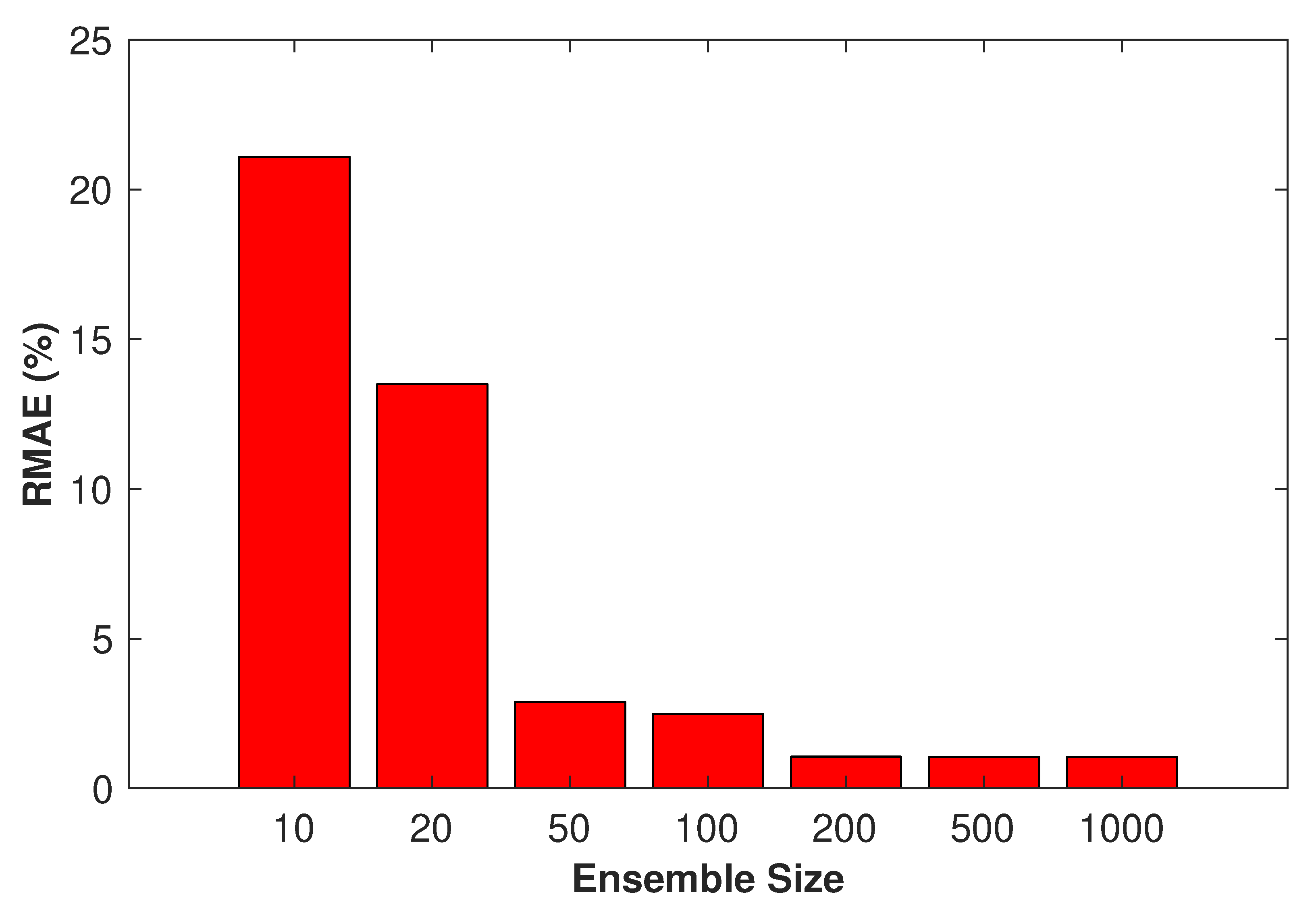
4.2. Sensitivity to Ensemble Size

We first study the sensitivity of the filter, to the ensemble size, $N_e$. Computing accurate state and parameter estimates with small ensembles is desirable to avoid an important increase in computational time. We run our assimilation system using seven ensemble sizes: $N_e=10$, 20, 50, 100, 200, 500, and 1000. Figure 2 presents the performance of the EnKF in terms of RMAE for the different ensemble sizes. As expected, increasing the ensemble size reduces the discrepancy between the estimates and the data. A clear improvement over the case with 20 ensemble members is observed. However, increasing the ensemble size beyond 200 members does not notably enhance the performance of the filter, although it dramatically increases the computational cost.

Figure 3 summarizes the assimilation results for the active, recovered, and confirmed cases obtained by the EnKF using 200 ensemble numbers. All results show a good fit between the predicted and observed values, with generally minor differences. The values of the model parameters estimated by the EnKF during the assimilation process are sketched in Figure 4. The parameters do not appear to be dramatically different from the initial values, except for the reproduction number and the recovery time. We observe a sharp increase in the reproduction number between March 1st and 15th. This number remains relatively high, almost $R_0=4$, during the pre-intervention period. During and after the intervention, the value of $R_0$ remains close to 1. That suggests that the intervention was very fruitful in controlling the pandemic. The recovery time increases significantly during the first two months, peaking at $16.1$, and remains constant after that. We also see a slight decrease in the time until death to $13.75$. The other parameters show slight deviations from the proposed initial values.

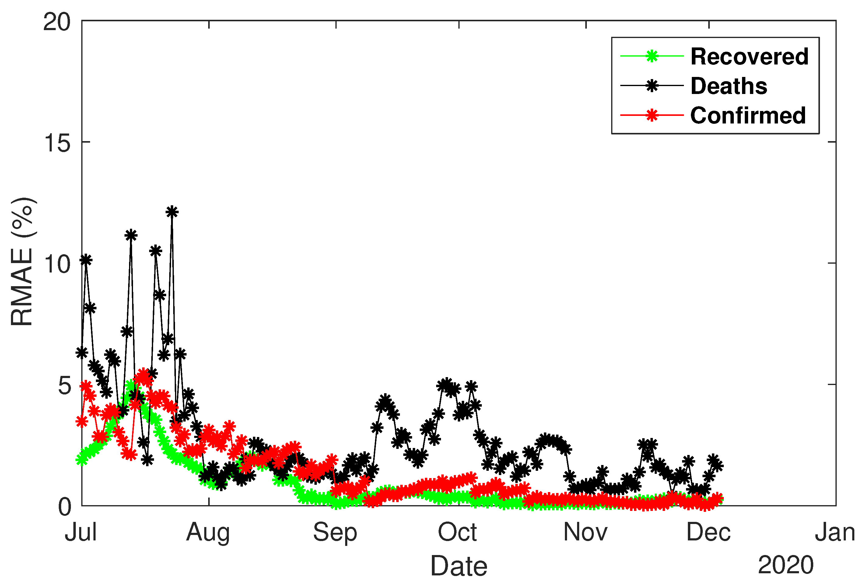
4.3. Predictability Experiment

To assess the system relevance for making short-term predictions, we daily performed two-week forecasts, starting from 1st July until 17th December (the day where the vaccination campaign started in Saudi Arabia). The estimated state and parameters during the assimilation process were used to conduct these forecasts. The RMAE of the deaths, and recovered and confirmed cases were then computed and plotted in Figure 5. The model performed very well. The values of the RMAE for the forecasted recovered and confirmed cases are always less than $5\%$, within the margin of the observation errors. Slightly higher RMAE are observed during the month of July for the death cases, reaching $12\%$. However, the model achieves a lower RMAE in the next few months, with an average of $3\%$.

Figure 6 shows the final predictions performed on 3rd December for the first two weeks of December. The predicted numbers of deaths, and recovered and confirmed cases are all in very good agreement with the data. While they perfectly match the data during the first 10 days, they tend to slightly underestimate or overestimate the observed values at the end of the second week. Overall, our numerical results demonstrate the capability of the proposed system in achieving an excellent two-week prediction skill.

4.4. Impact of Vaccination

On 17 December, Saudi Arabia started a three-phase COVID-19 vaccination program, thus becoming the first Arab country to roll out the Pfizer-BioNTech vaccine. The first phase targets people aged 65 and above, as well as people most exposed to the disease. The second phase will include people aged over 50, as well as those with specific chronic diseases, such as asthma and diabetes. The rest of the population will get the vaccine at the third stage. However, the Ministry has identified those who should not get the vaccine. They are women who are pregnant or breastfeeding, women who plan on getting pregnant in the next two months, people who suffer from severe allergic reactions, and those who have been infected by the virus in the past 90 days.

As of 17 January 2021, nearly 295,000 people have been vaccinated against COVID-19, according to the Saudi Health Council [52]. That gives $\alpha =3\times {10}^{-4}$. The Pfizer-BioNtech vaccine offers up to $95\%$ protection against Covid-19 after a second dose [53], which gives $\sigma =0.05$. We start our numerical simulation on 17 December for a period of six months with and without vaccination. Numerical results are presented in Figure 7, where $\alpha =0$ corresponds to the model output without vaccination. We notice that the current pace of vaccination does not show a significant decrease in the number of cases. We observe only a reduction of $9.02\%$ in the total confirmed cases, and $7.47\%$ in the total deaths. However, the vaccination rate is expected to increase in the upcoming weeks. Therefore, we consider three more different values of $\alpha$$\left(6\times {10}^{-4},1.2\times {10}^{-3},\mathrm{and}2.4\times {10}^{-3}\right)$. As we can see in Figure 7, intensifying the vaccination campaign starts to significantly decrease the number of cases. For $\alpha =0.0006$, we observe a reduction up to $16.08\%$ and $13.47\%$ for the total confirmed cases and deaths, respectively. Finally, a notable reduction is observed for $\alpha =0.0024$. Results show a decline by $38.67\%$ and $33.65\%$, respectively.

5. Conclusions

This paper presented an extended SEIR model with seven stages of infection, including vaccination, to simulate and predict the development of the novel COVID-19 outbreak. Initially, a mathematical analysis was carried out to illustrate the non-negativity, boundedness, epidemic equilibrium, existence, and uniqueness of the endemic equilibrium, and basic reproduction number of the proposed model. To mitigate the imperfection of SEIR models and the poorly known parameters, we first applied a data assimilation framework based on a Joint-EnKF for state-parameters estimation in order to enhance the model forecast skill. We assimilated real data of the number of deaths, the number of recovered cases, and the number of active cases. In the second step, the updated state and parameters were used to perform predictions two weeks ahead in order to assess the relevance of the system of making short-term predictions of the COVID-19 pandemic. Finally, we investigated the impact of vaccination on the spread of the disease.

The proposed methodology was validated with cases reported from Saudi Arabia. In the assimilation process, the estimated numbers of active, recovered, deaths, and confirmed cases were accurately predicted by the model, with generally minor differences. In the predictability experiments, the model provided encouraging results for short-term predictions, with a relatively small ensemble size. Moreover, model predictions can be updated weekly or every two weeks to accommodate short- and medium-term predictions. Results also show that intensifying the vaccination campaign significantly decreases the number of confirmed cases and deaths. The proposed model can serve as a tool for health authorities to plan, prepare, and take appropriate measures and decisions to control the pandemic.

References

1. World Health Organization (WHO). Coronavirus Disease (COVID-19) Outbreak Situation. Available online: https://www.who.int/emergencies/diseases/novel-coronavirus-2019 (accessed on 17 December 2020).
2. Kermack, W.O.; McKendrick, A.G. A contribution to the mathematical theory of epidemics. Proc. R. Soc. Lond. 1927, 115, 700–721. [Google Scholar]
3. Giraldo, J.O.; Palacio, D.H. Deterministic SIR (Susceptible–Infected–Removed) models applied to varicella outbreaks. Epidemiol. Infect. 2008, 136, 679–687. [Google Scholar] [CrossRef] [PubMed]
4. Fung, I.C.H. Cholera transmission dynamic models for public health practitioners. Emerg. Themes Epidemiol. 2014, 11, 1–11. [Google Scholar] [CrossRef] [Green Version]
5. Trawicki, M.B. Deterministic SEIRs epidemic model for modeling vital dynamics, vaccinations, and temporary immunity. Mathematics 2017, 5, 7. [Google Scholar] [CrossRef]
6. Bjørnstad, O.N.; Shea, K.; Krzywinski, M.; Altman, N.S. The SEIRS model for infectious disease dynamics. Nat. Methods 2020, 17, 557–558. [Google Scholar] [CrossRef]
7. Kumar, S.; Ahmadian, A.; Kumar, R.; Kumar, D.; Singh, J.; Baleanu, D.; Salimi, M. An efficient numerical method for fractional SIR epidemic model of infectious disease by using Bernstein wavelets. Mathematics 2020, 8, 558. [Google Scholar] [CrossRef] [Green Version]
8. Cooper, I.; Mondal, A.; Antonopoulos, C.G. A SIR model assumption for the spread of COVID-19 in different communities. Chaos Solitons Fractals 2020, 139, 110057. [Google Scholar] [CrossRef]
9. Bärwolff, G. Mathematical modeling and simulation of the COVID-19 pandemic. Systems 2020, 8, 24. [Google Scholar] [CrossRef]
10. Ndaïrou, F.; Area, I.; Nieto, J.J.; Torres, D.F. Mathematical modeling of COVID-19 transmission dynamics with a case study of Wuhan. Chaos Solitons Fractals 2020, 135, 109846. [Google Scholar] [CrossRef]
11. Sarkar, K.; Khajanchi, S.; Nieto, J.J. Modeling and forecasting the COVID-19 pandemic in India. Chaos Solitons Fractals 2020, 139, 110049. [Google Scholar] [CrossRef] [PubMed]
12. Ghil, M. Meteorological data assimilation for oceanographers. Part I: Description and theoretical framework. Dynam. Atmos. Ocean 1989, 13, 171–218. [Google Scholar] [CrossRef]
13. Holland, W.R.; Malanotte-Rizzoli, P. Assimilation of altimeter data into an ocean circulation model: Space versus time resolution studies. J. Phys. Oceanogr. 1989, 19, 1507–1534. [Google Scholar] [CrossRef] [Green Version]
14. Edwards, C.A.; Moore, A.M.; Hoteit, I.; Cornuelle, B.D. Regional ocean data assimilation. Ann. Rev. Mar. Sci. 2015, 7, 21–42. [Google Scholar] [CrossRef] [PubMed] [Green Version]
15. Hoteit, I.; Pham, D.T.; Blum, J. A simplified reduced order Kalman filtering and application to altimetric data assimilation in Tropical Pacific. J. Mar. Syst. 2002, 36, 101–127. [Google Scholar] [CrossRef]
16. Evensen, G. The ensemble Kalman filter: Theoretical formulation and practical implementation. Ocean Dyn. 2003, 53, 343–367. [Google Scholar] [CrossRef]
17. Kalman, R.E. A new approach to linear filtering and prediction problems. J. Mar. Syst. 1960, 82, 35–45. [Google Scholar] [CrossRef] [Green Version]
18. Altaf, M.; Butler, T.; Mayo, T.; Luo, X.; Dawson, C.; Heemink, A.; Hoteit, I. A comparison of ensemble Kalman filters for storm surge assimilation. Mon. Weather Rev. 2014, 142, 2899–2914. [Google Scholar] [CrossRef] [Green Version]
19. Buehner, M.; McTaggart-Cowan, R.; Heilliette, S. An ensemble Kalman filter for numerical weather prediction based on variational data assimilation: VarEnKF. Mon. Weather Rev. 2017, 145, 617–635. [Google Scholar] [CrossRef]
20. Raboudi, N.F.; Ait-El-Fquih, B.; Dawson, C.; Hoteit, I. Combining Hybrid and One-Step-Ahead Smoothing for Efficient Short-Range Storm Surge Forecasting with an Ensemble Kalman Filter. Mon. Weather Rev. 2019, 147, 3283–3300. [Google Scholar] [CrossRef]
21. Reichle, R.H.; McLaughlin, D.B.; Entekhabi, D. Hydrologic data assimilation with the ensemble Kalman filter. Mon. Weather Rev. 2002, 130, 103–114. [Google Scholar] [CrossRef] [Green Version]
22. Gharamti, M.; Kadoura, A.; Valstar, J.; Sun, S.; Hoteit, I. Constraining a compositional flow model with flow-chemical data using an ensemble-based Kalman filter. Water Resour. Res. 2014, 50, 2444–2467. [Google Scholar] [CrossRef] [Green Version]
23. Gharamti, M.; Ait-El-Fquih, B.; Hoteit, I. An iterative ensemble Kalman filter with one-step-ahead smoothing for state-parameters estimation of contaminant transport models. J. Hydrol. 2015, 527, 442–457. [Google Scholar] [CrossRef] [Green Version]
24. Ait-El-Fquih, B.; Gharamti, M.E.; Hoteit, I. A Bayesian consistent dual ensemble Kalman filter for state-parameter estimation in subsurface hydrology. Hydrol. Earth Syst. Sci. 2016, 20, 3289–3307. [Google Scholar] [CrossRef] [Green Version]
25. Khaki, M.; Ait-El-Fquih, B.; Hoteit, I.; Forootan, E.; Awange, J.; Kuhn, M. A two-update ensemble Kalman filter for land hydrological data assimilation with an uncertain constraint. J. Hydrol. 2017, 555, 447–462. [Google Scholar] [CrossRef] [Green Version]
26. Khaki, M.; Ait-El-Fquih, B.; Hoteit, I. Calibrating land hydrological models and enhancing their forecasting skills using an ensemble Kalman filter with one-step-ahead smoothing. J. Hydrol. 2020, 584, 124708. [Google Scholar] [CrossRef]
27. Hoteit, I.; Hoar, T.; Gopalakrishnan, G.; Collins, N.; Anderson, J.; Cornuelle, B.; Köhl, A.; Heimbach, P. A MITgcm/DART ensemble analysis and prediction system with application to the Gulf of Mexico. Dynam. Atmos. Ocean 2013, 63, 1–23. [Google Scholar] [CrossRef]
28. Triantafyllou, G.; Hoteit, I.; Luo, X.; Tsiaras, K.; Petihakis, G. Assessing a robust ensemble-based Kalman filter for efficient ecosystem data assimilation of the Cretan Sea. J. Mar. Syst. 2013, 125, 90–100. [Google Scholar] [CrossRef]
29. Gharamti, M.; Tjiputra, J.; Bethke, I.; Samuelsen, A.; Skjelvan, I.; Bentsen, M.; Bertino, L. Ensemble data assimilation for ocean biogeochemical state and parameter estimation at different sites. Ocean Model. 2017, 112, 65–89. [Google Scholar] [CrossRef]
30. Toye, H.; Kortas, S.; Zhan, P.; Hoteit, I. A fault-tolerant HPC scheduler extension for large and operational ensemble data assimilation: Application to the Red Sea. J. Comput. Sci. 2018, 27, 46–56. [Google Scholar] [CrossRef]
31. Yu, L.; Fennel, K.; Bertino, L.; El Gharamti, M.; Thompson, K.R. Insights on multivariate updates of physical and biogeochemical ocean variables using an Ensemble Kalman Filter and an idealized model of upwelling. Ocean Model. 2018, 126, 13–28. [Google Scholar] [CrossRef]
32. Neal, J.C.; Atkinson, P.M.; Hutton, C.W. Flood inundation model updating using an ensemble Kalman filter and spatially distributed measurements. J. Hydrol. 2007, 336, 401–415. [Google Scholar] [CrossRef]
33. Kimura, N.; Hsu, M.H.; Tsai, M.Y.; Tsao, M.C.; Yu, S.L.; Tai, A. A river flash flood forecasting model coupled with ensemble Kalman filter. J. Flood Risk Manag. 2016, 9, 178–192. [Google Scholar] [CrossRef]
34. Ziliani, M.G.; Ghostine, R.; Ait-El-Fquih, B.; McCabe, M.F.; Hoteit, I. Enhanced flood forecasting through ensemble data assimilation and joint state-parameter estimation. J. Hydrol. 2019, 577, 123924. [Google Scholar] [CrossRef]
35. Bettencourt, L.M.; Ribeiro, R.M.; Chowell, G.; Lant, T.; Castillo-Chavez, C. Towards real time epidemiology: Data assimilation, modeling and anomaly detection of health surveillance data streams. In NSF Workshop on Intelligence and Security Informatics; Springer: Berlin, Germany, 2007; pp. 79–90. [Google Scholar]
36. Rhodes, C.; Hollingsworth, T.D. Variational data assimilation with epidemic models. J. Theor. Biol. 2009, 258, 591–602. [Google Scholar] [CrossRef] [PubMed] [Green Version]
37. Gupta, H.; Verma, K.K.; Sharma, P. Using data assimilation technique and epidemic model to predict tb epidemic. Int. J. Comput. Appl. 2015, 128, 5. [Google Scholar] [CrossRef]
38. Eksin, C.; Paarporn, K.; Weitz, J.S. Systematic biases in disease forecasting – the role of behavior change. Epidemics 2019, 27, 96–105. [Google Scholar] [CrossRef] [PubMed]
39. Engbert, R.; Rabe, M.M.; Kliegl, R.; Reich, S. Sequential data assimilation of the stochastic SEIR epidemic model for regional COVID-19 dynamics. Bull. Math. Biol. 2021, 83, 1–16. [Google Scholar] [CrossRef]
40. Li, R.; Pei, S.; Chen, B.; Song, Y.; Zhang, T.; Yang, W.; Shaman, J. Substantial undocumented infection facilitates the rapid dissemination of novel coronavirus (SARS-CoV-2). Science 2020, 368, 489–493. [Google Scholar] [CrossRef] [PubMed] [Green Version]
41. Van Wees, J.D.; Osinga, S.; Van Der Kuip, M.; Tanck, M.W.; Tutu-van Furth, A. Forecasting hospitalization and ICU rates of the COVID-19 outbreak: An efficient SEIR model. Bull World Health Organ 2020. [Google Scholar] [CrossRef]
42. Evensen, G.; Amezcua, J.; Bocquet, M.; Carrassi, A.; Farchi, A.; Fowler, A.; Houtekamer, P.; Jones, C.K.; de Moraes, R.; Pulido, M.; et al. An international assessment of the COVID-19 pandemic using ensemble data assimilation. medRxiv 2020. [Google Scholar] [CrossRef]
43. Yang, Q.; Yi, C.; Vajdi, A.; Cohnstaedt, L.W.; Wu, H.; Guo, X.; Scoglio, C.M. Short-term forecasts and long-term mitigation evaluations for the COVID-19 epidemic in Hubei Province, China. Infect. Dis. Model. 2020, 5, 563–574. [Google Scholar]
44. Nkwayep, C.H.; Bowong, S.; Tewa, J.; Kurths, J. Short-term forecasts of the COVID-19 pandemic: Study case of Cameroon. Chaos Solitons Fractals 2020, 140, 110106. [Google Scholar] [CrossRef] [PubMed]
45. Sesterhenn, J.L. Adjoint-based data assimilation of an epidemiology model for the covid-19 pandemic in 2020. arXiv 2020, arXiv:2003.13071. [Google Scholar]
46. Armstrong, E.; Runge, M.; Gerardin, J. Identifying the measurements required to estimate rates of COVID-19 transmission, infection, and detection, using variational data assimilation. Infect. Dis. Model. 2020, 6, 133–147. [Google Scholar] [CrossRef]
47. Van den Driessche, P.; Watmough, J. Reproduction numbers and sub-threshold endemic equilibria for compartmental models of disease transmission. Math. Biosci. 2002, 180, 29–48. [Google Scholar] [CrossRef]
48. Diekmann, O.; Heesterbeek, J.A.P.; Metz, J.A. On the definition and the computation of the basic reproduction ratio R0 in models for infectious diseases in heterogeneous populations. J. Math. Biol. 1990, 28, 365–382. [Google Scholar] [CrossRef] [Green Version]
49. Martcheva, M. An Introduction to Mathematical Epidemiology; Springer: Berlin, Germany, 2015; Volume 61. [Google Scholar]
50. Saudi Center for Diseases Prevention and Control. Available online: https://covid19.cdc.gov.sa/daily-updates/ (accessed on 17 December 2020).
51. Saudi Ministry of Health. Available online: https://www.moh.gov.sa/en/Ministry/Statistics/Indicator/Pages/Indicator-1440.aspx (accessed on 17 December 2020).
52. Saudi Health Council. Available online: https://coronamap.sa (accessed on 19 January 2021).
53. Polack, F.P.; Thomas, S.J.; Kitchin, N.; Absalon, J.; Gurtman, A.; Lockhart, S.; Perez, J.L.; Pérez Marc, G.; Moreira, E.D.; Zerbini, C.; et al. Safety and efficacy of the BNT162b2 mRNA Covid-19 vaccine. N. Engl. J. Med. 2020, 383, 2603–2615. [Google Scholar] [CrossRef]
Figure 1. Disease transmission flow of the proposed model.
Mathematics 09 00636 g001
Figure 2. RMAE of the number of deaths as a function of ensemble size.
Mathematics 09 00636 g002
Figure 3. Assimilated numbers of: (a) Active cases. (b) Recovered cases. (c) Confirmed cases.
Mathematics 09 00636 g003
Figure 4. Time series of the estimated model parameters using the Joint-EnKF with 200 ensemble members. Initial and converged values for each parameter are also displayed.
Mathematics 09 00636 g004
Figure 5. RMAE of the daily two-week forecasts, starting from July 1st until December 3rd.
Mathematics 09 00636 g005
Figure 6. Predicted numbers of: (a) Recovered cases. (b) Death cases. (c) Confirmed cases for the first two weeks of December.
Mathematics 09 00636 g006
Figure 7. Impact of vaccination rate on the total number of: (a) Active cases. (b) Recovered cases. (c) Death cases. (d) Confirmed cases. α = 0 corresponds to the model output without vaccination.
Mathematics 09 00636 g007