
Stock Price Movement Prediction Based on a Deep Factorization Machine and the Attention Mechanism


School of Economics and Management, University of Science and Technology Beijing, Beijing 100083, China
*
Author to whom correspondence should be addressed.
Mathematics 2021, 9(8), 800; https://0-doi-org.brum.beds.ac.uk/10.3390/math9080800
Submission received: 17 March 2021
/
Revised: 26 March 2021
/
Accepted: 1 April 2021
/
Published: 7 April 2021
(This article belongs to the Special Issue Recent Progress in Big Data and Artificial Intelligence: Modern Methods and Applications)
Abstract
:The prediction of stock price movement is a popular area of research in academic and industrial fields due to the dynamic, highly sensitive, nonlinear and chaotic nature of stock prices. In this paper, we constructed a convolutional neural network model based on a deep factorization machine and attention mechanism (FA-CNN) to improve the prediction accuracy of stock price movement via enhanced feature learning. Unlike most previous studies, which focus only on the temporal features of financial time series data, our model also extracts intraday interactions among input features. Further, in data representation, we used the sub-industry index as supplementary information for the current state of the stock, since there exists stock price co-movement between individual stocks and their industry index. The experiments were carried on the individual stocks in three industries. The results showed that the additional inputs of (a) the intraday interactions among input features and (b) the sub-industry index information effectively improved the prediction accuracy. The highest prediction accuracy of the proposed FA-CNN model is 64.81%. It is 7.38% higher than that of traditional LSTM, and 3.71% higher than that of the model without sub-industry index as additional input features.
1. Introduction
The accurate prediction of stock price movement allows investors to make appropriate decisions and obtain excess returns. This remains a popular issue in academic and industrial fields due to the dynamic, highly sensitive, nonlinear and chaotic nature of stock prices [1]. As a binary classification task, the prediction of stock price movement is often explored using deep learning (DL) models, which have the advantages of automatic feature extraction and complex non-linear mapping ability [2]. The inputs of a DL model include the opening price, closing price, highest price, lowest price, trading volume and technical indicators (e.g., MA, RSI, MACD etc.) of a stock during a trading day [3,4]. We refer to these inputs as the ‘stock state’ in this paper. The DL model extracts the relevant features from this financial time series data and learns the sophisticated mapping relationship between these features and stock price movement. The output of the model is the probability that the stock price will rise at the predicted time point.
Among DL models, the long- and short-term memory (LSTM) neural network dominates in the field of time series forecasting because of its unique algorithm mechanism [5,6]. Although LSTM networks overcome the vanishing gradient problem found in traditional recurrent neural networks (RNNs), it is still a sequential-dependent computational method. The computational complexity of the LSTM model increases dramatically with the increase of the time series length. Further, the LSTM model treats all stock states equally at each moment. It therefore cannot effectively distinguish the important points of the time series. This is not conducive to learning the pattern of stock price movement, particularly when the input data contain noise. Existing studies of the LSTM model primarily focus on learning the changing pattern of stock states over a period of time, that is, the model is used to extract multiday temporal features from the input data. Most approaches to improve the model’s performance involve selecting important features from the stock state [7,8,9], yet very few pay attention to the intraday feature interactions (also known as ‘feature combinations’). It is reasonable to assume that a combination of different input features may have a stronger indicative effect on the prediction of stock price movement. For example, it is a common practice to use RSI combined with MACD to find an entry or exit point in the stock market. When they both indicate the stocks are oversold, it is more likely to be genuinely the entry point. Similarly, when they both generate overbought signals, it is probably the true exit point.
Data representation of the stock state is also of importance. Most previous studies in this field are based on the individual stock and its own historical attributes. However, the price movement of a single stock is often not isolated but rather affected by multiple related stocks [10].
In this paper, we seek solutions to these two above-mentioned problems. We propose a hybrid convolutional neural network based on a deep factorization machine and attention mechanism (FA-CNN) and a new stock state representation method to improve the prediction accuracy of stock price movement. The FA-CNN model consists of two independent modules: (1) a deep neural network based on the factorization machine DeepFM [11], which is used to (a) extract the intraday feature interactions of individual stock states and (b) find their optimal weights without traditional feature engineering; and (2) a convolutional neural network based on an attention mechanism (ATT-CNN), which is used to (a) extract the multiday temporal features of input data, and (b) focus on important input data by allocating an attention weight for each stock state. Furthermore, because price co-movement between an individual stock and the stock index enhances after a stock is selected to be added into the stock index [12], we use the stock index as supplementary information for the individual stock.
2. Literature Review
Techniques from previous research on improving the prediction accuracy of stock price movement can be categorized into two groups: (1) improving data representation, which involves selecting and converting important stock information into input data; and (2) building deep learning models with stronger feature learning ability, which involves effectively extracting features from the input data. We now present these two research streams in turn.
2.1. Data Representation
Information related to the rise and fall of stock prices is selected to represent the stock state at each time point. This information is then converted into numerical data that can be directly fed into the model. Most existing studies represent the current stock state as a vector containing the stock price and technical indicators. As such, the model’s input is a matrix formed by a chronologically ordered series of stock states [13,14,15]. Kim and Kim [16] and Vidal and Kristjanpoller [17] expanded the input data representation by transforming the historical stock prices over a period of time into an image. However, they focused only on a single stock, and not on related stocks or information pertaining to the overall market.
Behavioral finance believes that investors’ sentiments, irrational behaviors and other non-fundamental factors lead to the co-movement of stock prices, that is, the phenomenon where price changes occur in the same direction among individual stocks or between individual stocks and the market. When Claessens and Yafeh [12] carried out research on 10 years of data on 40 developed and emerging markets, they found that in most markets, when added to a major index, firms experienced an increase in the extent to which market returns explained firms’ stock returns. This demonstrated the value of referring to stock index information when predicting individual stock trends. Many studies have confirmed the existence of stock price co-movement in the stock market [18,19,20], but few have used this to predict the direction of stock price movement. Hoseinzade and Haratizadeh [21] proposed a CNN-based framework that takes information from different markets and uses it to predict the future of those markets. They focused on the superiority of the proposed framework but did not verify whether adding information from other stock markets was more effective than using only a single stock market as the input in stock price trend forecasting. Thus, in this paper we use the stock index as a form of supplementary information to expand the data representation of the stock state. We then verify whether this strategy can improve the prediction accuracy of our model.
2.2. Deep Learning Models
Deep learning models are usually regarded as feature extractors and classifiers for stock price prediction. Some literatures [22,23,24] reviewed the recent deep learning applications in financial field and found that the LSTM neural networks, convolutional neural networks (CNNs) and their hybrid models are commonly used deep learning models for stock market predictions.
The LSTM neural network is an improved version of the traditional RNN [25]. It alleviates the vanishing gradient problem of the RNN by setting three gate variables to control how much information of the previous time step is transmitted to the current time step. Thus, the LSTM neural network is effective at capturing temporal features on sequential data, and its hybrid models are widely used for the prediction of time series data [26,27,28]. Fischer and Krauss [29] used an LSTM network to predict the rise and fall of the S&P 500 index. Their results showed that the prediction accuracy of the LSTM model was significantly higher than that of random forest, deep neural network (DNN) and logistic regression models. Nabipour et al. [30] used ten kinds of technical indicators as inputs to predict the future trend of the German stock market group. They compared the performance of a variety of traditional machine learning models and deep learning models such as DNN, RNN and LSTM. Their results showed that the LSTM algorithm had the highest accuracy; however, because the computation of each step for the LSTM algorithm is suspended until the complete execution of the previous step, it is significantly slower than other parallel computing structures [31].
The CNN was proposed by Lecun et al. [32] for the image classification task. Taken its advantage of translation invariance, the CNN can recognize the object no matter where it is in the image. This characteristic makes the CNN particularly suitable for detecting the key time point in sequential data, and it overcomes the sequential-dependent problem of traditional RNNs. Kim [33] later applied the CNN to the sentence classification task, and Zhang and Wallace [34] experimented to further explain the influence of various CNN parameters on sequential data classification. Since then, the CNN has been widely used to tackle time series data because of its advantages of (a) parallel computation and (b) having less parameters than the LSTM network. Selvin et al. [35] compared the performance of LSTM, CNN and RNN models on predicting the short-term rise and fall of stock prices with financial time series data as model inputs. Their results showed that the prediction accuracy of the CNN model was higher than that of the other two models. Long et al. [36] created a multi-filters neural network (MFNN) model to extract temporal features from time series data at the same time. Their results showed that the MFNN model performed better than either the LSTM or CNN models alone and other traditional machine learning models. Alonso-Monsalve et al. [37] compared the performance of four different network architectures—the CNN, hybrid CNN-LSTM network, multilayer perceptron and radial basis function neural network—in the domain of trend classification of cryptocurrency exchange rates. Their results suggested that hybrid CNN-LSTM neural networks significantly outperformed all the rest, while CNNs were also able to provide good results. All the above studies showed the feasibility of the CNN in the prediction of time series data. However, the traditional CNN model is unable to distinguish the importance of extracted features, that is, in order to fully extract features from the input data, the number of CNN filters is usually set to be redundant, which leads to the derived feature maps having different levels of importance.
The attention mechanism was first proposed in the field of computer vision [38], then flourished in the field of machine translation [39,40]. It imitates the signal processing mechanism of the human brain, allocating computing resources to more important tasks. Liu et al. [41] used an attention-based capsule network to quantify the impact of different events on the prediction of stock price movement, and Chen and Ge [42] built an attention-based LSTM model to predict the movements of Hong Kong stock prices. Qiu et al. [43] integrated wavelet transform, LSTM and an attention mechanism to predict the value of Standard & Poor’s 500 Composite Stock Price Index, Dow Jones Industrial Average and Hang Seng Index. Results showed that the attention-based LSTM model performed better than Gate Recurrent Unit (GRU) model. Such research demonstrates that the attention mechanism can enhance the prediction accuracy of the baseline model. However, when the attention mechanism is integrated with complex models such as the LSTM and capsule network, it also significantly increases the parameters, which may cause overfitting problems. In the field of image classification, Woo et al. [44] proposed a lightweight and general module—a convolutional block attention module (CBAM)—to make the CNN model focus only on important features and suppress unnecessary ones. Their results showed that a CBAM can be integrated into a variety of classic CNN structures, and it achieved better classification results than the original structure with negligible overheads. Applying an attention-based CNN model to the financial field is of great importance due to the advantages of its lightweight computation and its ability to distinguish important information.
The above studies lay out how to extract the temporal features of input data more effectively, but they all ignore mining the input features themselves. A combination of different input features could be used as a new feature for prediction, which may have a stronger indicative effect on predicting the trend of stock price movement. In the field of advertising recommendation, it was found that users usually download apps for food delivery at mealtimes, which indicated that the (order-2) interaction between app category and timestamp could be used as a new feature for the click-through rate (CTR) prediction. The DeepFM model—an end-to-end model that learns sophisticated feature interactions behind user click behaviors—was proposed to improve the accuracy of CTR prediction for the recommender system [11]. This model was then later used by Huang et al. [45] to learn the high- and low-order feature interactions between stock price data and text embedding. Their results showed that the DeepFM model performed better than a traditional DNN model. However, they only focused on the stock state before the prediction rate and did not consider the temporal features. Zhou et al. [46] proposed an empirical mode decomposition and factorization machine based neural network (EMD2FNN) model to predict the value of several stock indices. They combined factorization machine with neural networks to capture the factorized interactions between features. However, the work focused on comparing the performance of EMD2FNN model with that without EMD layer. It did not elaborate on the importance of factorization machine in improving the model’s prediction accuracy.
In summary, in this paper we aim to improve the prediction of stock price movement by (a) expanding the data representation by adding the stock index as supplementary information, and (b) building a novel FA-CNN model which extracts the intraday feature interactions and the multiday temporal features more effectively.
The rest of this paper is organized as follows. In Section 3, we formulized the task of stock price movement prediction and introduced the structure and computation processing of our proposed FA-CNN model. In Section 4, we described the data processing method and metrices. Further, the experimental results of comparative models were analyzed in detail. Finally, we concluded this work and present some future avenues of research in Section 5.
3. Methodology
3.1. Problem Formulization
The prediction of stock price movement can be regarded as a supervised binary classification task. The label of a sample represents the uptrend or downtrend of a stock on trading day t, as shown in Equation (1). The goal of our model is to make the predicted label as close as possible to the real label of the sample:
Since we take the co-movement of stock price and stock index into account, the input data is concatenated by the vectors and . These are arranged in ascending order of time, representing the state of individual stock and the stock index at day , respectively. Each element of or represents the price or technical indicators of the stock or stock index at day :
The output of the model refers to the probability that the closing price of stock will rise on trading day compared with that on trading day . The definition is shown in Equation (3), where Function (∙) is the specific calculation process of the model, which is described in detail in Section 3.2:
The is the true label probability distribution of samples, and the is the proposed model’s predicted label probability distribution of samples. The objective of the model is to find the optimal parameters to make the most approximate to the , that is, to minimize the cross-entropy loss function. Cross-entropy [47] is commonly used to define a loss function in machine learning. The objective function is defined in Equation (4):
In Equation (4), denotes the number of individual stocks and denotes the number of trading days.
3.2. Model Design
3.2.1. Overall Structure of FA-CNN Model
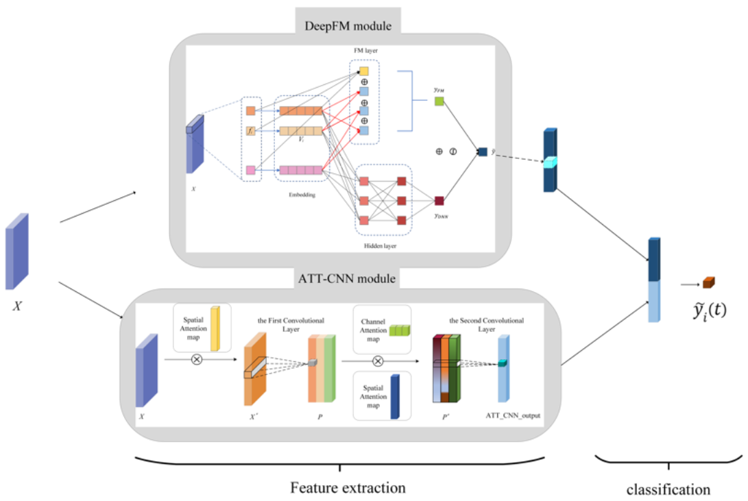
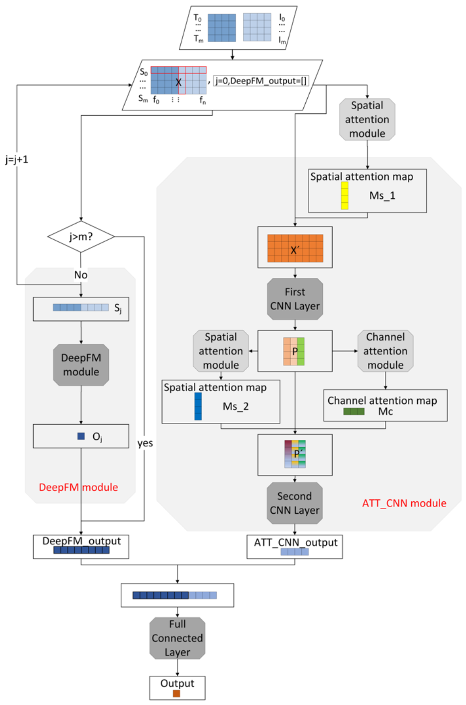
In this section, we introduce our proposed FA-CNN hybrid model in detail. The overall structure of the model is shown in Figure 1. The feature extraction part of the model can be divided into two independent modules: (1) the DeepFM module, for automatically extracting intraday feature interactions, as detailed in Section 3.2.2; and (2) the ATT-CNN module, for extracting multiday temporal features, as detailed in Section 3.2.3. The outputs of these two modules are concatenated and fed to the last full connection layer for classification. In order to explain the model prediction process more clearly, Figure 2 was drawn to show how the model get the prediction results step by step. Combined with Figure 1, the proposed FA-CNN hybrid model can be easily understood.
3.2.2. DeepFM Module
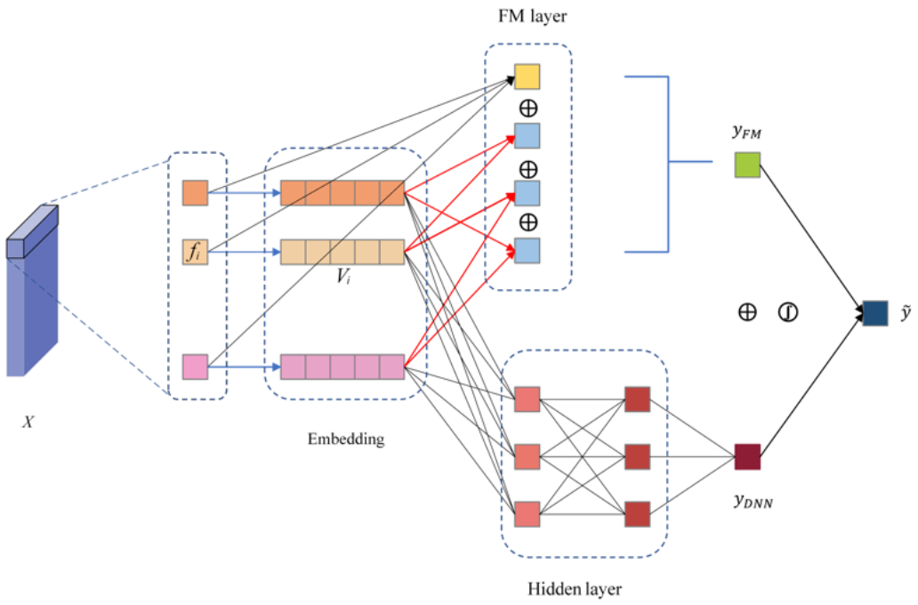
DeepFM [11] consists of two layers—the FM layer and the deep layer—that share the same input. The FM layer extracts the low-order (order-1 and order-2) feature interactions of the input data to get . The deep layer extracts the high-order feature interactions to get . These two outputs are then added and activated to obtain as the output of the DeepFM module, as shown in Equation (5):
The advantage of DeepFM is that it can learn the feature interactions of different orders without feature engineering. Its detailed calculation process is shown in Figure 3.
Output is defined as:
where: is the th dimensional element of or , , ; the first part, , is a linear (order-1) interaction among features, and is the weight to be learned; the second part, , is the pairwise (order-2) feature interactions, and the pairwise weight, , which measures the importance of the interactions of features and , is the inner product of their latent vectors and , . Thus, Equation (6) can be converted to Equation (7):
If is repeated and formed into a new vector, , that has the same dimensions with vector , Equation (6) can be further converted to Equation (8):
where denotes the element-wise multiplication of and . Note, the blue arrow in Figure 3 shows the calculation steps, and the matrix formed by is called Embedding.
The DNN part learns the high-order feature interactions and takes the Embedding generated by the FM part as the input. The Embedding is also denoted as in Equation (9). The output of the th hidden layer in the DNN is denoted as in Equation (10), where and are the parameters. The final output, , is defined as Equation (11), where H is the number of hidden layers:
3.2.3. ATT-CNN Module
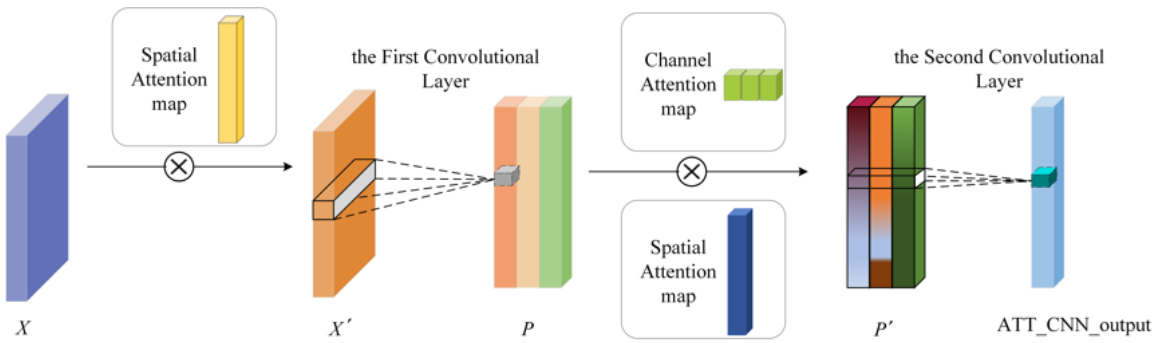
In this paper, we modify the original CBAM module [46] to enhance the ability of the CNN to recognize the important points in the time series data. The overall structure of the ATT-CNN module is shown in Figure 4.
The th row vector of input matrix (denoted as X in Figure 4) represents the stock state at time . Intuitively, the state near the current time or the state with obvious trend change may have a greater impact on stock price movement at the current time. Therefore, the spatial attention module is used to calculate the weight for each time point. The adjusted is then fed into a CNN for temporal feature pattern extraction. The row vector is an indivisible unit due to its representation of the stock state. Thus, the size of filters is set to be , where is the length of the time window and is the dimension of the row vector in the input matrix. Many feature maps are obtained using different filters after convolutional operation, but not every feature map is of the same importance. Therefore, the channel attention module is used to calculate the weight for each feature map. The matrix , adjusted by the channel attention map and spatial attention map, is finally fed to another CNN to get the output. The concise expression of the above calculation process is shown in Equations (12)–(15):
Spatial Attention in ATT-CNN Module
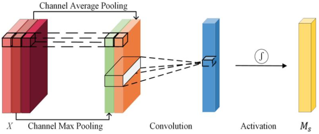
As shown in Figure 5, the spatial attention map focuses on telling the network which row of input matrix carries more important information. It performs average pooling and max pooling for each position in input matrix channel-dimensionally. After the pooling operation, the results are stacked and fed into the CNN with a filter size, where w is the dimension of the row vector in the input matrix. As such, the model treats the stock state vector as a whole instead of as the original filter size of 7 × 7. Finally, the result is activated by sigmoid function to make the elements in range from 0 to 1, representing the importance of the corresponding time point. The calculation process of is shown in Equation (16):
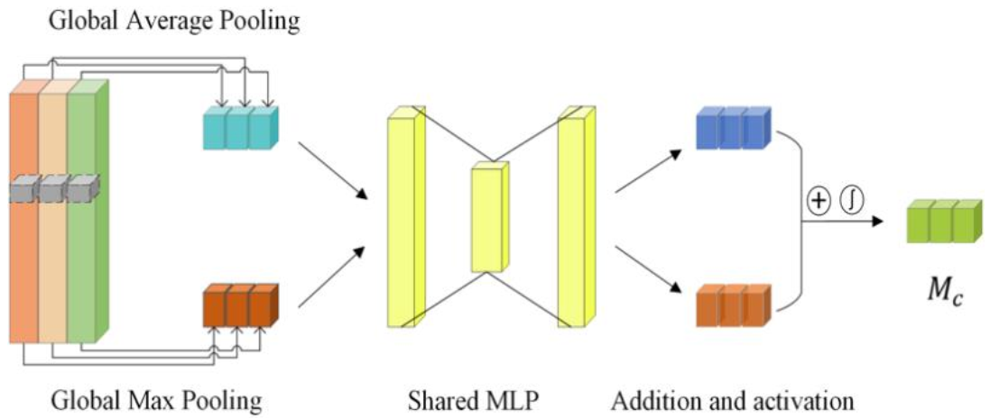
Channel Attention in ATT-CNN Module
As shown in Figure 6, the channel attention map focuses on telling the network which feature map carries more important information. In contrast to the spatial attention module, this module uses global average pooling and global max pooling to compress each feature map into vectors and , respectively, with the same size of C × 1 × 1, where C is the number of channels. Vectors and can be regarded as the intuitive interpreter of each feature map. Both vectors are fed to a shared two-layer fully connected neural network to obtain the nonlinear maps. Finally, these two maps are added and activated by sigmoid function to make sure each element in is between 0 and 1, which represents the importance of the corresponding channel. The calculation process of is shown in Equation (17):
4. Experiments
4.1. Data Selection
As mentioned in Section 2.1, we assumed that adding the stock index as supplementary feature can help improve the prediction accuracy of models. This is actually based on the premise that the stock price of the individual stock is mainly affected by the environment within the studied industry, but not by the other industries. Because if an industry has strong co-movement with many other industries, it seems inadequate to add only one industry index as supplementary input to improve prediction accuracy. In addition, literature [48] has shown that co-movement exists among stock indices in Chinese stock market. Therefore, it needs to find out whether the chosen industry has strong co-movement with other industries before the experiment.
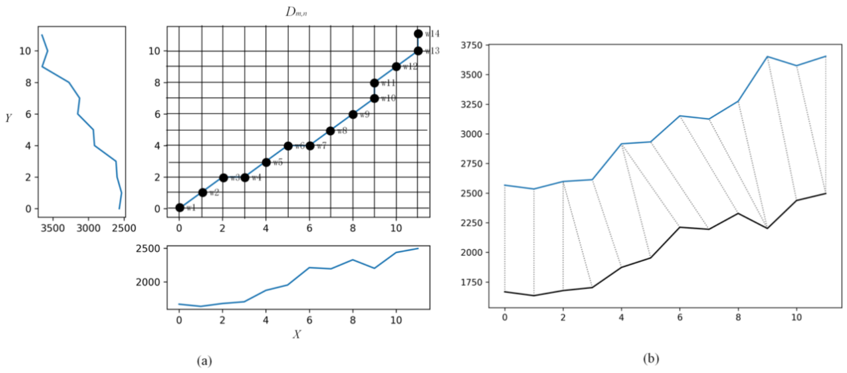
Obviously, if one time series co-moves with another, some similarity must exist in their morphologic. Therefore, the co-movement strength between industries was measured by the morphological similarity between industry indices. Dynamic time warping (DTW) algorithm proposed by Berndt and Clifford [49] is an appropriate method to calculate the similarity between two time series. It overcomes the matching defect caused by the one-to-one correspondence of the points in Euclidean distance, so that the points in two time series can be ‘one to many’ matched, and it also has a strong recognition effect on the amplitude change of time series. Using DTW to calculate the similarity of two time series can be summarized in Algorithm 1. It is actually the process of using dynamic programming algorithm to find the shortest path. The dtw-python package was used to implement this DTW algorithm.
| Algorithm 1. Dynamic time warping algorithm. |
| Input: and . |
| Output:, the best wrapping path with the minimum cumulative distance . |
Step1: As shown in Figure 7a, construct a cost matrix , where the element denotes the Euclidean distance . The element of the wrapping, path denotes the location of a pair of points from and in . And the constraints of are as follows:
|
| Step2: Initialize the cumulative distance: |
| Step3: Calculate the minimum cumulative distance according to the recursive formula: . |
| Step4: Trace back to find all the matching point pairs in the wrapping path as shown in Figure 7b. |
The Shenwan first-class industry indices were chosen to analyze the co-movement between industries. The indices are released by Shenwan Hongyuan Securities and are highly recognized by investors and researchers [50,51]. The co-movement levels between industries are shown in Figure 8. The darker the color, the weaker co-movement the two industries are.
It showed that some industries have strong co-movement with other industries whereas some industries have weak co-movement. Therefore, the stocks in three representative industries—Food and Beverage, Health Care and Real Estate industries—which respectively had the weak, medium and strong co-movement with other industries were taken to test our proposed method. Since there are many individual stocks in each industry, it is necessary to select the respective ones. The stocks in a series of sub-industry indices released by China Securities Index Co., Ltd. (Shanghai, China) meet our needs. The sub-industry index selects stocks with large market capitalization and good liquidity from the first-class industry, reflecting the overall trend of each sub-industry in the Chinese A-shares market. Thus, the data from Food & Beverage Sub-industry (FBSI 000815), Health Care Sub-industry (HCSI 000814) and Real Estate Sub-industry (RESI 000816) were gathered, covering the period from 1 July 2017 to 31 November 2020. The input data include the historical prices and technical indicators of both individual stock and sub-industry index. The number of samples and label distributions of the three datasets are showed in Table 1. The label distribution of three datasets is relatively balanced, which can make the trained model not be biased to any label.
4.2. Data Pre-Processing
The features in stock state vectors and are explained in detail in Appendix B. They primarily include stock price data, trading volume, money and various technical indicators as calculated by the Python tool TA-lib.
Different stocks have different opening, closing, highest and lowest prices, and there is a large gap among the mean and variance of these prices. This is harmful to the convergence of training models. It was therefore necessary to normalize these input features before they were fed into our model. It is unreasonable to directly normalize time series data in a period of time because the earlier data will use the future information. We therefore adopted a normalized rolling method that was similar to the training method, that is, for each stock, at the last time point in the sliding window, we calculated the mean and variance of each feature of input data within the sliding window and used this to normalize the original feature. This operation, as shown in Equation (18), ensured that no normalized data used future information. Finally, the standardized was fed into the model. In this way, each feature in the input data obeys the standard normal distribution, which is good for model convergence:
In Equation (18), is the th feature of stock on trading day , and are the respective mean and standard deviation of the th feature of stock within a sliding window containing consecutive days.
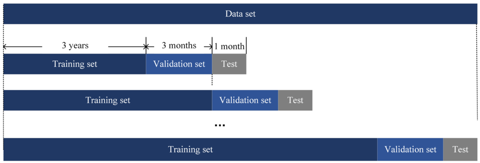
As the input data is sequential, we used the training technique of incremental learning. As shown in Figure 9, the initial training set covered a period of three years, the validation set covered a period of three months and the test set covered a period of one month. Thereafter, the sliding window moved three months ahead, step by step, until the model test in the final month. This kind of technique allows the model to account for the most recent trends of stock price movements and patterns. We used the average measurement of multiple test sets as the final result of our model.
4.3. Metrics
Two metrics were used to measure the performance of different models: accuracy, as shown in Equation (19); and the Matthews correlation coefficient (MCC), as shown in Equation (20). Accuracy measures the model’s ability to correctly predict all classes of labeled data, and MCC [–1, 1] is a correlation coefficient between the real and predicted labels of samples for binary classifications in machine learning. It takes into account true and false positives and negatives and it is generally regarded as a balanced measure even if the two classes are of different sizes. It means that when the MCC value is 1, the predicted label distribution is completely consistent with the real label distribution, and when the MCC value is −1, the opposite is true:
In Equations (19) and (20), TP is the number of the samples whose real and predicted labels are both positive, TN is the number of the samples whose real and predicted labels are both negative, FN is the number of the samples whose real label is positive but the predicted label is negative, and FP is the number of the samples whose real label is negative but the predicted label is positive.
4.4. Comparative Models and Parameter Settings
The LSTM model is the commonly used deep learning model that uses financial time series data as the input for the prediction of stock price movement. As such, we used this model as our baseline. Additionally, to verify the effectiveness of the DeepFM and ATT-CNN modules we proposed in Section 3.2, we conducted experiments on the following models: (1) the LSTM + DeepFM control model, where we sought to verify whether adding the DeepFM module to extract intraday feature interactions can improve the prediction accuracy; (2) the ATT-CNN control model, where we sought to verify whether a CNN module based on an attention mechanism can replace the LSTM model to extract multiday temporal features of financial series data; (3) the multi-filters neural network (MFNN) model, a hybrid model proposed by Long et al. [37], used here as the state-of-the-art work; and (4) our proposed hybrid model, the FA-CNN model. As stated in Section 1, we took the co-movement between individual stock and the stock index into consideration when predicting stock price movement. To verify whether this strategy can effectively improve the prediction accuracy, we performed the five models listed above under two different strategies: Strategy 1, where the input data contain only the financial information of the individual stock; and Strategy 2, where the input data contain the financial information of both the individual stock and its stock index. These models were trained separately for each industry.
All the comparative models were implemented by TensorFlow. The optimizer used for training the models is Adam with learning rate 0.001. Regarding to the FA-CNN model hyperparameters, the latent dimension of FM layer is 10. Three different filter windows [3, 66], [5, 66], [10, 66] were used in the first convolutional layer and [5, 1] in the second convolutional layer, and each convolutional layer has 32 units. The last full-connected layer has 64 units. As for the baseline LSTM model, it has 128 LSTM units. The MFNN was constructed as the literature [37] showed.
4.5. Results and Analysis
The results of the five different models for test data under each of the two strategies are shown in Table 2.
As shown in Table 2, the performance of the different models under Strategy 2 was consistently higher than that under Strategy 1. This suggests that enriching the individual stock state representation with the stock index information helps improve the accuracy of stock price movement prediction. This is perhaps because the stock index is influenced by the performance of other competing companies, which indirectly and comprehensively reflects the development of the whole industry. Therefore, investors perhaps refer to the stock index to make investment decisions, which results in a certain price co-movement between individual stock and the stock index. This is in line with the explanation of stock price co-movement in behavioral finance theory. In addition, it also showed that the degree of improved prediction accuracy is different among these three different industries. The accuracy of the food and beverage sub-industry is improved much better than that of the real estate sub-industry after taking the sub-industry index as additional input. This is possibly caused by the different levels of co-movement with other industries. The price of the stock in the real estate industry is not only influenced by the other counterparts but also greatly influenced by its own upstream and downstream affiliates in other industries such as banking, architectural materials and so on. Therefore, as for the stocks in the industry strongly co-moving with many other industries, it is probably not adequate to only add one industry index as an additional input to improve the prediction accuracy. The more comprehensive information is considered, the higher the accuracy of prediction can be achieved.
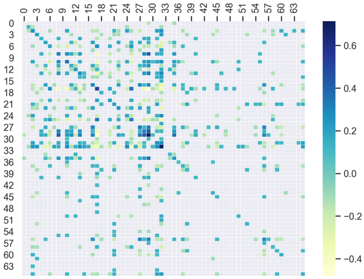
The LSTM + DeepFM model performed better than the LSTM model under both strategies. This indicates that adding the extraction of intraday feature interactions of input data can indeed provide valuable information in improving the prediction accuracy. To clearly reveal the impact of feature interactions, the latent Embedding matrix in the DeepFM module after training for health care sub-industry was taken out as an example to compute the feature interaction weight matrix , where is the transposition of . The weight matrix with size 66 × 66 is shown in Figure 10. This is a symmetrical matrix, where the absolute value of the weight represents the importance of feature interactions. In the heat map in Figure 9, the darker the color, the greater the weight. The feature index is shown in Appendix A, with a total of 33 features containing stock prices and technical indicators. In Figure 10, the first 33 features are of the individual stock, and the following 33 features are of the stock index. To show the results more clearly, the weight values in the range of [−0.1, 0.1] (i.e., those which are of less importance) were covered up. The diagonal elements of the matrix represent the weight of features itself. This shows that almost all the features of individual stocks had an important indicative effect on the result, while fewer features of the stock index had an important impact on the result. In addition, (a) most feature interactions of greater importance were distributed in the interaction area of the individual stock itself, (b) fewer of these interactions were distributed in the interaction area of the individual stock and the stock index, and (c) the fewest interactions were distributed in the interaction area of the stock index itself. This is consistent with our intuitive understanding about the impact of price co-movement between individual stocks and the stock index, and it also explains why adding relevant information of the stock index can increase the prediction accuracy of the model. Besides, it was found interestingly that some technical indicators combination shown in Figure 10 was consistent with that adopted by traders in the real world. For example, the Bollinger Bands in conjunction with MACD signals can be used in trending markets to find an entry or exit point. The MACD is an effective trend-following and momentum indicator and can be used to assess if a trend is picking up or slowing down. While Bollinger Bands measure the volatility of stock prices and can be used as an entry trigger and subsequent confirmation of a trade. Usually, the traders identify the trend using MACD signal and use the lower (upper) band as a stop loss in an uptrend (downtrend). As the Figure 10 showed, the MACD signal (feature 13) had greater weights with Upper band (feature 6) and Lower band (feature 8) than that with other features. This explains why extracting the intraday feature interactions of input features can effectively improve the prediction accuracy.
The ATT-CNN model performed better than the LSTM model under both strategies, which shows that a CNN with an attention mechanism is more effective at extracting temporal features. In Section 3.2, we explained that the spatial attention can compute the relevance between the stock state at each time point and stock price movement. As shown in Figure 11, we randomly selected a sample to visualize this relevance, where the price performance of the selected sample with stock code 000432 is shown as candlestick charts, and the input time span is from 31 August 2018 to 11 August 2018. Note the background color of Figure 11 represents the relevance between the stock state at each time point and stock price movement. As the input data had long time steps (66 time steps), the LSTM model was unable to effectively transfer the influence of the faraway points to the current predicted time point. In contrast, our proposed ATT-CNN model has the ability to compute the weight of each time point no matter how long the time step is. As such, this model performed better than the LSTM model in extracting the temporal features. Note that most of the important time points were near or far away from the predicted time point. This is likely a coincidence, as the attention weight is only related to the stock state rather than the position of the time point.
Our proposed FA-CNN model performed best among these models, which suggests that the two modules in our proposed model were not in conflict and worked together to improve the accuracy of the model. The prediction accuracy of each constituent stock in FBSI is listed in Appendix B, which shows that the stocks with longer listing time and larger market capitalization tend to have higher prediction accuracy. Perhaps, this is because the listing company with a longer listing time and higher market capitalization owns a higher market acceptance and less irrational investment. It needs further study to find out the true cause.
5. Conclusions and Future Works
In this paper, we proposed a convolutional neural network model based on a deep factorization machine and attention mechanism (FA-CNN) for the prediction of stock price movement using financial time series data. The main contributions of our paper can be summarized as follows:
- 1)
- Price co-movement between the individual stock and the stock index should be taken into consideration when predicting the trend of individual stock prices. Using the stock index information as additional input features can enrich the data representation of the stock state and thereby improve the prediction accuracy of the model. In addition, the degree of improved accuracy is related to the strength of the co-movement between the studying industry and other industries. The more independent the industry is, the stronger the effect of taking industry index as additional input on improving prediction accuracy. These suggestions were validated by our experimental results, and they extend the data representation of the stock state.
- 2)
- In contrast to previous studies, we extracted the intraday feature interactions of the stock state using the DeepFM module. We then verified that mining these intraday feature interactions can effectively improve the prediction accuracy of the model. This broadens the methods of feature mining with financial time series data.
- 3)
- We used an attention-based convolutional neural network (ATT-CNN) module to extract multiday temporal features. This module can process time series data with any length, and it can distinguish the importance of the stock state at different time points, which is very important for accurately predicting stock price movement. Comparative experiments showed that the ATT-CNN module performed better than the LSTM and CNN models.
In this paper, the super parameter window size of input data has not been studied in detail. For short-term stock forecasting, the optimal time window size can help the model achieve a better result. Further, we had noticed that it was inadequate to only add one industry index as an input feature to improve the prediction accuracy of those stocks that had strong price co-movement with multiple industries. However, adding all the relevant industry indices as input features will sharply increase the dimension of input data, which may lead to redundant features. How to balance the input features and prediction accuracy will be the next studying point.
Author Contributions
Conceptualization, methodology, software, X.Z. (Xiaodong Zhang) and S.L.; validation and formal analysis, X.Z. (Xin Zheng); writing—original draft preparation, X.Z. (Xiaodong Zhang) and S.L.; writing—review and editing, X.Z. (Xiaodong Zhang); visualization, S.L.; supervsion, project administration and funding acquisition, X.Z. (Xiaodong Zhang). All authors have read and agreed to the published version of the manuscript.
Funding
This research was funded by National Natural Science Foundation of China, grant number 71871018.
Institutional Review Board Statement
Not applicable.
Informed Consent Statement
Not applicable.
Data Availability Statement
Restrictions apply to the availability of these data. Data was obtained from https://www.joinquant.com/ (accessed on 12 December 2020) and are available with the permission of https://www.joinquant.com/ (accessed on 12 December 2020).
Conflicts of Interest
The authors declare no conflict of interest.
Abbreviations
| FA-CNN | convolutional neural network based on deep factorization machine and attention mechanism |
| ATT-CNN | convolutional neural network based on attention mechanism |
| CBAM | convolutional block attention module |
| CNN | convolutional neural networks |
| CTR | click-through rate |
| DeepFM | deep factorization machines |
| DL | deep learning |
| DNN | deep neural network |
| DTW | dynamic time warping |
| EMD | empirical mode decomposition |
| EMD2FNN | empirical mode decomposition and factorization machine based neural network |
| FBSI | food and beverage sub-industry |
| FC layer | full-connected layer |
| HCSI | health care sub-industry index |
| LSTM | long- and short-term memory |
| MA | moving average |
| MACD | moving average convergence divergence |
| MCC | matthews correlation coefficient |
| MFNN | multi-filters neural network |
| RESI | real estate sub-industry |
| RNN | recurrent neural networks |
| RSI | relative strength index |
Appendix A

Table A1.
Stock prices and technical indicators included as input features.
| Index | Features | Description | |
|---|---|---|---|
| 0 | Open price | - | |
| 1 | Close price | - | |
| 2 | High price | - | |
| 3 | Low price | - | |
| 4 | Volume | - | |
| 5 | Money | - | |
| 6 | Bollinger Bands | Upper band | An indicator of overbought or oversold conditions. |
| 7 | Middle band | ||
| 8 | Lower band | ||
| 9 | Exponential Moving Average | An indicator more responsive to changes in the data. | |
| 10 | Double Exponential Moving Average | A smoothing indicator with less lag than a straight exponential moving average. | |
| 11 | Triple Exponential Moving Average | The T3 is a type of moving average, or smoothing function. | |
| 12 | Moving Average Convergence Divergence | MACD | The Moving Average Convergence Divergence (MACD) is the difference between two Exponential Moving Averages. The MACD signals trend changes and indicates the start of new trend direction. High values indicate overbought conditions, and low values indicate oversold conditions. |
| 13 | MACD signal | ||
| 14 | MACD hist | ||
| 15 | Money Flow Index | An indicator ranging from 0 to 100. Values above 80 /below 20 indicate tops/bottoms. | |
| 16 | Momentum | An indicator that shows if prices are increasing at an increasing rate or decreasing at a decreasing rate. | |
| 17 | Average Directional Movement Index | A Welles Wilder-style moving average of the Directional Movement Index. | |
| 18 | Rate of change | A momentum-based technical indicator that measures the percentage change in price between the current price and the price a certain number of periods ago. | |
| 19 | Relative Strength Index | The RSI ranges from 0 to 100. The RSI is interpreted as an overbought/oversold indicator when the value is over 70/below 30. | |
| 20 | Commodity Channel Index | An indicator designed to detect beginning and ending market trends. | |
| 21 | 1-day ROC of a triple smooth EMA | An oscillator used to identify oversold and overbought market. | |
| 22 | Williams’ %R | Values range from 0 to 100, and are charted on an inverted scale, that is, with 0 at the top and 100 at the bottom. | |
| 23 | Balance of Power | An oscillator that represents the battle between the bulls and the bears in the market. | |
| 24 | Absolute Price Oscillator | A MACD, but it can use any time periods. | |
| 25 | Average Directional Movement Index Rating (ADXR) | An average of the two ADX values filtering out excessive tops and bottoms. | |
| 26 | Average Directional Movement Index (ADX) | A Welles Wilder-style moving average of the Directional Movement Index. | |
| 27 | Ultimate Oscillator | The weighted sum of three oscillators of different time periods. The values of the Ultimate Oscillator range from 0 to 100. Values over 70 indicate overbought conditions, and values under 30 indicate oversold conditions. | |
| 28 | Chaikin A/D Line | The Accumulation/Distribution Line is similar to the On Balance Volume (OBV), which sums the volume times +1/-1 based on whether the close is higher than the previous close. | |
| 29 | Chaikin A/D Oscillator | The oscillator measures the accumulation-distribution line of moving average convergence-divergence (MACD). | |
| 30 | On Balance Volume | The OBV is a cumulative total of the up and down volume. When the close is higher than the previous close, the volume is added to the running total, and when the close is lower than the previous close, the volume is subtracted from the running total. | |
| 31 | Average True Range | A measure of volatility. | |
| 32 | True Range | A base calculation that is used to determine the normal trading range of a stock or commodity. | |
Appendix B
Table A2.
Prediction accuracy of constituent stocks in Food and Beaverage sub-industry Index (FBSI).
Table A2.
Prediction accuracy of constituent stocks in Food and Beaverage sub-industry Index (FBSI).
| Stock Code | Market Capitalization (A Hundred Million) | Listing Time | Accuracy |
|---|---|---|---|
| 000568 | 1.28 | 09/05/1994 | 0.6667 |
| 000596 | 1.7 | 02/09/1996 | 0.7019 |
| 000729 | 5.87 | 16/07/1997 | 0.6438 |
| 000799 | 4.4 | 18/07/1997 | 0.7143 |
| 000848 | 1.93 | 13/11/1997 | 0.7714 |
| 000858 | 11.8 | 27/04/1998 | 0.6743 |
| 000860 | 4.13 | 04/11/1998 | 0.619 |
| 000869 | 6.4 | 26/10/2000 | 0.6762 |
| 002216 | 5.07 | 30/01/2008 | 0.781 |
| 002304 | 27 | 27/10/2009 | 0.7095 |
| 002461 | 4.06 | 18/08/2010 | 0.6814 |
| 002481 | 5.97 | 21/09/2010 | 0.5762 |
| 002507 | 5.6 | 23/11/2010 | 0.7286 |
| 002568 | 5.2 | 25/03/2011 | 0.6286 |
| 002570 | 18.1 | 12/04/2011 | 0.6286 |
| 002626 | 8.05 | 28/10/2011 | 0.5238 |
| 002847 | 2.83 | 08/02/2017 | 0.5218 |
| 300146 | 15 | 15/12/2010 | 0.619 |
| 300401 | 1.59 | 09/10/2014 | 0.5776 |
| 600059 | 3.09 | 16/05/1997 | 0.671 |
| 600073 | 4 | 04/07/1997 | 0.6281 |
| 600132 | 2.22 | 30/10/1997 | 0.6667 |
| 600197 | 4.7 | 16/09/1999 | 0.7333 |
| 600298 | 4.16 | 18/08/2008 | 0.619 |
| 600305 | 2.84 | 06/02/2001 | 0.6762 |
| 600519 | 22.4 | 27/08/2001 | 0.7619 |
| 600559 | 1.74 | 29/10/2002 | 0.6386 |
| 600597 | 9.75 | 28/08/2002 | 0.6857 |
| 600600 | 6.38 | 27/08/1993 | 0.7621 |
| 600779 | 1.27 | 06/12/1996 | 0.6238 |
| 600809 | 2.73 | 06/01/1994 | 0.619 |
| 600872 | 2.24 | 24/01/1995 | 0.7238 |
| 600873 | 1.05 | 17/02/1995 | 0.681 |
| 600882 | 0.495 | 06/12/1995 | 0.6062 |
| 600887 | 1.02 | 12/03/1996 | 0.7208 |
| 603027 | 3.68 | 24/03/2016 | 0.5714 |
| 603043 | 6.59 | 27/06/2017 | 0.5286 |
| 603198 | 9.44 | 28/05/2015 | 0.619 |
| 603288 | 38.4 | 11/02/2014 | 0.5997 |
| 603369 | 8.77 | 03/07/2014 | 0.6143 |
| 603589 | 9.6 | 29/06/2015 | 0.581 |
| 603866 | 6.19 | 22/12/2015 | 0.5714 |
| 603919 | 7.66 | 10/03/2016 | 0.5238 |
References
- Bukhari, A.H.; Raja, M.A.Z.; Sulaiman, M.; Islam, S.; Shoaib, M.; Kumam, P. Fractional Neuro-Sequential ARFIMA-LSTM for Financial Market Forecasting. IEEE Access 2020, 8, 71326–71338. [Google Scholar] [CrossRef]
- Li, A.W.; Bastos, G.S. Stock Market Forecasting Using Deep Learning and Technical Analysis: A Systematic Review. IEEE Access 2020, 8, 185232–185242. [Google Scholar] [CrossRef]
- Chande, T. Adapting Moving Averages to Market Volatility. Tech. Anal. Stock. Commod. 1992, 10, 108–114. [Google Scholar]
- Rosillo, R.; Fuente, D.; Brugos, J.A. Technical analysis and the Spanish stock exchange: Testing the RSI, MACD, momentum and stochastic rules using Spanish market companies. Appl. Econ. 2013, 45, 1541–1550. [Google Scholar] [CrossRef]
- Sezer, O.B.; Gudelek, M.U.; Ozbayoglu, A.M. Financial time series forecasting with deep learning: A systematic literature review: 2005–2019. Appl. Soft Comput. 2020, 90, 106–181. [Google Scholar] [CrossRef] [Green Version]
- Torres, J.F.; Hadjout, D.; Sebaa, A.; Martinez-Alvarez, F.; Troncoso, A. Deep Learning for Time Series Forecasting: A Survey. Big Data 2020. [Google Scholar] [CrossRef]
- Pehlivanlı, A.Ç.; Aşıkgil, B.; Gülay, G. Indicator selection with committee decision of filter methods for stock market price trend in ISE. Appl. Soft Comput. 2016, 49, 792–800. [Google Scholar] [CrossRef]
- Naik, N.; Mohan, B.R. Optimal Feature Selection of Technical Indicator and Stock Prediction Using Machine Learning Technique. In Emerging Technologies in Computer Engineering: Microservices in Big Data Analytics; Springer: Singapore, 2019; pp. 261–268. [Google Scholar]
- Yuan, X.; Yuan, J.; Jiang, T.; Ain, Q.U. Integrated Long-Term Stock Selection Models Based on Feature Selection and Machine Learning Algorithms for China Stock Market. IEEE Access 2020, 8, 22672–22685. [Google Scholar] [CrossRef]
- Kwon, Y.; Choi, S.; Moon, B. Stock prediction based on financial correlation. In Proceedings of the Genetic and Evolutionary Computation Conference, Washington, DC, USA, 25–29 June 2005; pp. 2061–2066. [Google Scholar]
- Guo, H.; TANG, R.; Ye, Y.; Li, Z.; He, X. DeepFM: A Factorization-Machine based Neural Network for CTR Prediction. In Proceedings of the Twenty-Sixth International Joint Conference on Artificial Intelligence, Melbourne, Australia, 19–25 August 2017; pp. 1725–1731. [Google Scholar]
- Claessens, S.; Yafeh, Y. Comovement of Newly Added Stocks with National Market Indices: Evidence from Around the World. Rev. Financ. 2012, 17, 203–227. [Google Scholar] [CrossRef]
- Shynkevich, Y.; McGinnity, T.M.; Coleman, S.A.; Belatreche, A.; Li, Y. Forecasting price movements using technical indicators: Investigating the impact of varying input window length. Neurocomputing 2017, 264, 71–88. [Google Scholar] [CrossRef] [Green Version]
- Chong, E.; Han, C.; Park, F.C. Deep learning networks for stock market analysis and prediction: Methodology, data representations, and case studies. Expert Syst. Appl. 2017, 83, 187–205. [Google Scholar] [CrossRef] [Green Version]
- Lee, S.W.; Kim, H.Y. Stock market forecasting with super-high dimensional time-series data using ConvLSTM, trend sampling, and specialized data augmentation. Expert Syst. Appl. 2020, 161, 113704. [Google Scholar] [CrossRef]
- Kim, T.; Kim, H.Y. Forecasting stock prices with a feature fusion LSTM-CNN model using different representations of the same data. PLoS ONE 2019, 14, e212320. [Google Scholar] [CrossRef]
- Vidal, A.; Kristjanpoller, W. Gold volatility prediction using a CNN-LSTM approach. Expert Syst. Appl. 2020, 157, 113481. [Google Scholar] [CrossRef]
- Greenwood, R. Excess Comovement of Stock Returns: Evidence from Cross-Sectional Variation in Nikkei 225 Weights. Rev. Financ. Stud. 2008, 21, 1153–1186. [Google Scholar] [CrossRef]
- Gul, F.; Kim, J.; Qiu, A. Ownership Concentration, Foreign Shareholding, Audit Quality, and Stock Price Synchronicity: Evidence from China. J. Financ. Econ. 2010, 95, 425–442. [Google Scholar] [CrossRef]
- López-García, M.N.; Sánchez-Granero, M.A.; Trinidad-Segovia, J.E.; Puertas, A.M.; De Las Nieves, F.J. Volatility Co-Movement in Stock Markets. Mathematics 2021, 9, 598. [Google Scholar] [CrossRef]
- Hoseinzade, E.; Haratizadeh, S. CNNpred: CNN-based stock market prediction using a diverse set of variables. Expert Syst. Appl. 2019, 129, 273–285. [Google Scholar] [CrossRef]
- Nosratabadi, S.; Mosavi, A.; Duan, P.; Ghamisi, P.; Filip, F.; Band, S.; Reuter, U.; Gama, J.; Gandomi, A.H. Data Science in Economics: Comprehensive Review of Advanced Machine Learning and Deep Learning Methods. Mathematics 2020, 8, 1799. [Google Scholar] [CrossRef]
- Ozbayoglu, A.M.; Gudelek, M.U.; Sezer, O.B. Deep learning for financial applications: A survey. Appl. Soft Comput. 2020, 93, 106384. [Google Scholar] [CrossRef]
- Hu, Z.; Zhao, Y.; Khushi, M. A Survey of Forex and Stock Price Prediction Using Deep Learning. Appl. Syst. Innov. 2021, 4, 9. [Google Scholar] [CrossRef]
- Hochreiter, S.; Schmidhuber, J. Long Short-Term Memory. Neural Comput. 1997, 9, 52100701–52101780. [Google Scholar] [CrossRef] [PubMed]
- Karim, F.; Majumdar, S.; Darabi, H.; Chen, S. LSTM Fully Convolutional Networks for Time Series Classification. IEEE Access 2017, 6, 1662–1669. [Google Scholar] [CrossRef]
- Kim, H.Y.; Won, C.H. Forecasting the volatility of stock price index: A hybrid model integrating LSTM with multiple GARCH-type models. Expert Syst. Appl. 2018, 103, 25–37. [Google Scholar] [CrossRef]
- Cao, J.; Li, Z.; Li, J. Financial time series forecasting model based on CEEMDAN and LSTM. Phys. A Stat. Mech. Appl. 2019, 519, 127–139. [Google Scholar] [CrossRef]
- Fischer, T.; Krauss, C. Deep learning with long short-term memory networks for financial market predictions. Eur. J. Oper. Res. 2018, 270, 654–669. [Google Scholar] [CrossRef] [Green Version]
- Nabipour, M.; Nayyeri, P.; Jabani, H.; Mosavi, A.; Salwana, E.S.S. Deep Learning for Stock Market Prediction. Entropy 2020, 22, 840. [Google Scholar] [CrossRef]
- Lei, T.; Zhang, Y.; Wang, S.I.; Dai, H.; Artzi, Y. Simple Recurrent Units for Highly Paralleizable Recurrence. arXiv 2017, arXiv:1709.02755. [Google Scholar]
- LeCun, Y.; Bengio, Y. Convolutional networks for images, speech, and time series. In The Handbook of Brain Theory and Neural Networks; The MIT press: Cambridge, MA, USA, 1998; pp. 255–258. [Google Scholar]
- Kim, Y. Convolutional Neural Networks for Sentence Classification. In Proceedings of the 2014 Conference on Empirical Methods in Natural Language Processing, Doha, Qatar, 26–28 October 2014; pp. 1746–1751. [Google Scholar]
- Zhang, Y.; Wallace, B. A Sensitivity Analysis of (and Practitioners’ Guide to) Convolutional Neural Networks for Sentence Classification. arXiv 2015, arXiv:1510.03820. [Google Scholar]
- Selvin, S.; Vinayakumar, R.; Gopalakrishnan, E.A.; Menon, V.K.; Soman, K.P. Stock price prediction using LSTM, RNN and CNN-sliding window model. In Proceedings of the 2017 International Conference on Advances in Computing, Communications and Informatics (ICACCI), Udupi, India, 13–16 September 2017; pp. 1643–1647. [Google Scholar]
- Long, W.; Lu, Z.; Cui, L. Deep learning-based feature engineering for stock price movement prediction. Knowl. Based Syst. 2019, 164, 163–173. [Google Scholar] [CrossRef]
- Alonso-Monsalve, S.; Suárez-Cetrulo, A.L.; Cervantes, A.; Quintana, D. Convolution on neural networks for high-frequency trend prediction of cryptocurrency exchange rates using technical indicators. Expert Syst. Appl. 2020, 149, 113250. [Google Scholar] [CrossRef]
- Mnih, V.; Heess, N.; Graves, A.; Kavukcuoglu, K. Recurrent Models of Visual Attention. Advances in Neural Information Processing Systems. arXiv 2014, arXiv:1406.6247. [Google Scholar]
- Bahdanau, D.; Cho, K.; Bengio, Y. Neural Machine Translation by Jointly Learning to Align and Translate. arXiv 2015, arXiv:1409.0473. [Google Scholar]
- Vaswani, A.; Shazeer, N.; Parmar, N.; Uszkoreit, J.; Jones, L.; Gomez, A.N.; Kaiser, Ł.; Polosukhin, I. Attention is All you Need. arXiv 2017, arXiv:1706.03762. [Google Scholar]
- Liu, J.; Lin, H.; Yang, L.; Xu, B.; Wen, D. Multi-Element Hierarchical Attention Capsule Network for Stock Prediction. IEEE Access 2020, 8, 143114–143123. [Google Scholar] [CrossRef]
- Chen, S.; Ge, L. Exploring the attention mechanism in LSTM-based Hong Kong stock price movement prediction. Quant. Financ. 2019, 19, 1507–1515. [Google Scholar] [CrossRef]
- Qiu, J.; Wang, B.; Zhou, C. Forecasting stock prices with long-short term memory neural network based on attention mechanism. PLoS ONE 2020, 15, e227222. [Google Scholar] [CrossRef]
- Woo, S.; Park, J.; Lee, J.; Kweon, I.S. CBAM: Convolutional Block Attention Module. In Proceedings of the Computer Vision ECCV 2018, Munich, Germany, 8–14 September 2018; pp. 3–19. [Google Scholar]
- Huang, J.; Zhang, X.; Fang, B. CoStock: A DeepFM Model for Stock Market Prediction with Attentional Embeddings. In Proceedings of the 2019 IEEE International Conference on Big Data (Big Data), Los Angeles, CA, USA, 9–12 December 2019; pp. 5522–5531. [Google Scholar]
- Zhou, F.; Zhou, H.; Yang, Z.; Yang, L. EMD2FNN: A strategy combining empirical mode decomposition and factorization machine based neural network for stock market trend prediction. Expert Syst. Appl. 2019, 115, 136–151. [Google Scholar] [CrossRef]
- Rubinstein, R. The Cross-Entropy Method for Combinatorial and Continuous Optimization. Methodol. Comput. Appl. 1999, 1, 127–190. [Google Scholar] [CrossRef]
- Chen, H.; Zheng, X.; Zeng, D.D. Analyzing the co-movement and its spatial–temporal patterns in Chinese stock market. Phys. A Stat. Mech. Its Appl. 2020, 555, 124655. [Google Scholar] [CrossRef]
- Berndt, D.; Clifford, J. Using Dynamic Time Warping to Find Patterns in Time Series. In Proceedings of the 3rd International Conference on Knowledge Discovery and Data Mining, Seattle, WA, USA, 31 July–1 August 1994; pp. 359–370. [Google Scholar]
- Chen, J.; Xie, C.; Zeng, Z. A Combination of Hidden Markov Model and Association Analysis for Stock Market Sector Rotation. Rev. Cercet. Interv. Soc. 2018, 63, 149–165. [Google Scholar]
- Qiao, F. Study on Price Fluctuation of Industry Index in Chinas Stock Market Based on Empirical Mode Decomposition. Asian Econ. Financ. Rev. 2020, 10, 559–573. [Google Scholar] [CrossRef]
Figure 1.
The structure of the FA-CNN model.

Figure 2.
The prediction process of the FA-CNN model.

Figure 3.
The structure of the DeepFM module.

Figure 4.
The structure of the ATT-CNN module.

Figure 5.
The computation operation of the spatial attention module.

Figure 6.
The computation operation of the channel attention module.

Figure 7.
(a) An example process of finding wrapping path; (b) An example of final wrapping path.

Figure 8.
The co-movement level between industries.

Figure 9.
Time series dataset splitting method.

Figure 10.
Weight matrix of 2-order feature combination.

Figure 11.
Spatial attention weight of a sample.

Table 1.
Label distributions of three datasets.
| Dataset | Numbers of Samples | Positive Proportion | Negative Proportion |
|---|---|---|---|
| HCSI | 40114 | 50.90% | 49.10% |
| FBSI | 31244 | 51.57% | 48.43% |
| RESI | 33563 | 53.03% | 46.97% |
Table 2.
The performance of different models with different strategies.
| Model | HCSI Average Accuracy | HCSI Average MCC | FBSI Average Accuracy | FBSI Average MCC | RESI Average Accuracy | RESI Average MCC | |
|---|---|---|---|---|---|---|---|
| Strategy 1: where input data contain only the individual information | LSTM | 0.5495 | 0.1544 | 0.5633 | 0.1813 | 0.5443 | 0.1428 |
| LSTM + DeepFM | 0.5541 | 0.1544 | 0.5766 | 0.1933 | 0.5438 | 0.1525 | |
| ATT-CNN | 0.5634 | 0.1799 | 0.5833 | 0.2167 | 0.5720 | 0.1686 | |
| MFNN [28] | 0.5643 | 0.1803 | 0.5959 | 0.2233 | 0. 5729 | 0.1691 | |
| FA-CNN | 0.5931 | 0.1847 | 0.6110 | 0.2368 | 0.5803 | 0.1899 | |
| Strategy 2: where input data contain both the individual information and the industry index information | LSTM | 0.5670 | 0.1627 | 0. 5743 | 0.2376 | 0.5643 | 0.1567 |
| LSTM + DeepFM | 0.5895 | 0.1690 | 0. 5929 | 0.2616 | 0.5773 | 0.1563 | |
| ATT-CNN | 0.5955 | 0.1857 | 0.6174 | 0.3716 | 0.5824 | 0.1737 | |
| MFNN [28] | 0.5988 | 0.2019 | 0.6295 | 0.3783 | 0.5883 | 0.1900 | |
| FA-CNN | 0.6190 | 0.2976 | 0.6481 | 0.4218 | 0.5938 | 0.2139 |
Publisher’s Note: MDPI stays neutral with regard to jurisdictional claims in published maps and institutional affiliations. |
© 2021 by the authors. Licensee MDPI, Basel, Switzerland. This article is an open access article distributed under the terms and conditions of the Creative Commons Attribution (CC BY) license (https://creativecommons.org/licenses/by/4.0/).
Share and Cite
MDPI and ACS Style
Zhang, X.; Liu, S.; Zheng, X. Stock Price Movement Prediction Based on a Deep Factorization Machine and the Attention Mechanism. Mathematics 2021, 9, 800. https://0-doi-org.brum.beds.ac.uk/10.3390/math9080800
AMA Style
Zhang X, Liu S, Zheng X. Stock Price Movement Prediction Based on a Deep Factorization Machine and the Attention Mechanism. Mathematics. 2021; 9(8):800. https://0-doi-org.brum.beds.ac.uk/10.3390/math9080800
Chicago/Turabian StyleZhang, Xiaodong, Suhui Liu, and Xin Zheng. 2021. "Stock Price Movement Prediction Based on a Deep Factorization Machine and the Attention Mechanism" Mathematics 9, no. 8: 800. https://0-doi-org.brum.beds.ac.uk/10.3390/math9080800
Note that from the first issue of 2016, this journal uses article numbers instead of page numbers. See further details here.