
Comparisons of Parallel Systems with Components Having Proportional Reversed Hazard Rates and Starting Devices


1
Department of Mathematics and Statistics, McMaster University, Hamilton, ON L8S 4L8, Canada
2
Department of Statistics, University of Zabol, Zabol 98615-538, Sistan and Baluchestan, Iran
3
Department of Mathematics, University of Zabol, Zabol 98615-538, Sistan and Baluchestan, Iran
*
Author to whom correspondence should be addressed.
Mathematics 2021, 9(8), 856; https://doi.org/10.3390/math9080856
Submission received: 4 February 2021
/
Revised: 24 March 2021
/
Accepted: 8 April 2021
/
Published: 14 April 2021
(This article belongs to the Special Issue Reliability and Statistical Learning and Its Applications)
Abstract
:In this paper, we consider stochastic comparisons of parallel systems with proportional reversed hazard rate (PRHR) distributed components equipped with starting devices. By considering parallel systems with two components that PRHR and starting devices, we prove the hazard rate and reversed hazard rate orders. These results are then generalized for such parallel systems with n components in terms of usual stochastic order. The establish results are illustrated with some examples.
1. Introduction
Comparison of important characteristics of lifetimes of technical systems is of interest in many problems. Let be non-negative independent random variables representing lifetimes of components of a system. Let be independent Bernoulli random variables with if the i-th component survives from random shocks and if the i-th component fails from the shocks and , for . Further, let them also be independent of s. For a given time period, we can then use to denote the lifetimes of components that are subject to random shocks. Of special interest are and corresponding to lifetimes of parallel and series systems, respectively. Throughout this work, we use the term “heterogeneity” to mean that components have different lifetime distributions. A similar assumption is also made on the survival probabilities. It is then of natural interest to evaluate the influence of heterogeneity among the components and the random shocks on the lifetimes of parallel and series systems, and this reliability problem forms the main basis for the present work.
We can present a different motivation for this problem as follows. Consider a finite system with each of its components equipped with a starter whose performance is modelled by a Bernoulli random variable, and with all component lifetimes being independent. As a starter may fail to initiate the component, the total number of components in operation would thus be random. Such situations arise naturally in a number of applications. Some possible examples are as follows: start-ups of power plants with gas turbines, length of time of a conference online being the maximum online time of those who successfully register for the conference, and the maximum loss of an insured individual who has a policy covering multiple risks being the maxima of those invoked losses. Another interesting scenario discussed by [1,2] in auction theory is when an auctioneer attracts some predetermined potential bidders by advertising a valuable object; in this case, the largest bid of those participants defines the price of the object for sale. One may additionally refer to [3,4,5,6] for the role of random extremes in financial economics, reliability theory, actuarial science, hydrology, and so on.
In actuarial set-up, the claims sizes may be represented by variables s, and the variables s represent their occurrences. In this case, and correspond to the largest and smallest claim amounts in a portfolio of risks, respectively.
Considerable attention has been paid in the actuarial literature to different stochastic comparisons of numbers of claims and aggregate claim amounts. In particular, [7] consider a general scale model and discuss orderings of smallest and largest claim amounts, while [8] focus on the comparison of smallest and largest claim amounts from two sets of heterogeneous portfolios. These authors have specifically discussed the ordering results in the presence of heterogeneity among the sample sizes and the probabilities of claims and also in the presence of dependence between claim sizes and probabilities of claims.
The flexible family of distributions offered by the proportional reversed hazard rate (PRHR) model has found key applications in lifetime data analysis. For a system consisting of n components, let and (for ) denote the lifetime and the reversed hazard rate of the i-th component. Then, when
the variables s are said to have the model, where is referred to as the baseline reversed hazard rate function and s (all positive) are the proportionality constants. It is then easy in this case to see that , the distribution function of , is given by , , where is the baseline distribution function corresponding to . The PRHR family of distributions include many commonly used lifetime distributions as special cases such as generalized exponential and exponentiated Weibull distributions. In addition, when the proportionality constants s are integers, then s are in fact the lifetimes of parallel systems consisting of components with their lifetimes being independent and identically distributed with distribution function As parallel systems with more components are less prone to failure, the PRHR model is also referred to as resilience model in the reliability literature; one may refer to [9] for relevant details.
Suppose , Then, the survival function of series systems, , is given by
Similarly, the survival function of is given by
Then, the stochastic comparison between and is equivalent to the comparison between and . It should be mentioned that the comparison between and has been investigated by many authors earlier. For this reason, we have not considered this problem in the present work.
In this paper, we consider only stochastic comparisons of parallel systems with proportional reversed hazard rate (PRHR) distributed components equipped with starting devices. We specifically establish the hazard rate, reversed hazard rate and usual stochastic orders of parallel systems with PRHR distributed components equipped with starting devices.
The rest of this paper is organized as follows. In Section 2, we present some basic definitions and notation pertaining to stochastic orders and majorization orders that are used in the present work. Section 3 discusses stochastic comparisons of parallel systems for different probabilities of starters in terms of hazard rate order. In Section 4, stochastic comparisons of parallel systems are established for different probabilities of starters in terms of reversed hazard rate order. Section 5 discusses stochastic comparisons of parallel systems for different probabilities of the starters in terms of usual stochastic order. Finally, some concluding remarks are made in Section 6.
2. Preliminaries
In this section, we present some basic definitions and lemmas that will be useful for all subsequent developments. For convenience, we use the notation to denote that both sides of an equality have the same sign.
Definition 1.
Suppose X and Y are two non-negative continuous random variables with distribution functions and survival functions and hazard rate functions and , and reversed hazard rate functions and . We assume that all involved expectations exist. Then:
- (i)
- X is said to be larger than Y in the usual stochastic order (denoted by if for all This is equivalent to saying that for all increasing functions
- (ii)
- X is said to be larger than Y in the hazard rate order (denoted by if and only if increases in This is equivalent to saying that for all
- (iii)
- X is said to be larger than Y in the reversed hazard rate order (denoted by if and only if increases in This is equivalent to saying that for all
It is known that the usual stochastic order is included in both hazard rate and reversed hazard rate orders. The books by [10,11] provide elaborate details on various stochastic orders and their applications to a wide array of problems.
Definition 2.
Consider two vectors and with corresponding increasing arrangements and , respectively. Then:
- (i)
- a is said to majorize denoted by if for and ;
- (ii)
- a is said to weakly submajorize denoted by if for .
The concept of majorization is a way of comparing two vectors of the same dimension, in terms of the dispersion of their components, in which the order means that s are more dispersive than s for a fixed sum. For example, we always have where with . It is evident that the majorization order implies weak submajorization order.
Definition 3.
A real-valued function ϕ, defined on a set , is said to be Schur-convex on if
Further, ϕ is said to be Schur-concave function on if is Schur-convex on
Lemma 1.
([12], p. 84) Suppose is an open interval and is continuously differentiable. Then, necessary and sufficient conditions for ϕ to be Schur-convex (Schur-concave) on are
- (i)
- ϕ is symmetric on ;
- (ii)
- for all and all ,where denotes the partial derivative of ϕ with respect to its i-th argument.
Lemma 2.
([12], p. 87) Consider the real-valued function defined on a set . Then, implies if and only if ϕ is increasing and Schur-convex on
3. Hazard Rate Order
In this section, we discuss stochastic comparisons of parallel systems for different probabilities of starters in terms of hazard rate order.
Theorem 1.
Suppose and are independent non-negative random variables with . Further, suppose , , , and are independent Bernoulli random variables, independently of s, with and , . Let and . Then, the following statements hold true:
- (i)
- If () and ( ), then
- (ii)
- If , then
Proof.
- (i)
- The survival functions of and are given byandFor the necessity part, note that implies that and so . We thus haveTherefore, we getwhich implies that . Now, for the sufficiency part, let us considerand it is then enough to show that is increasing in x. Upon differentiating with respect to x, we getFor proving the increasing property of , it is enough to show thatis positive. For this purpose, we findLet us now consider . Then, we have ; since , we findand so is decreasing. Consequently, for , and so . Thus, Part (i) of the theorem is proved.
- (ii)
- The survival functions of and , for , areandrespectively. Then, it is enough to show thatis increasing in x. We can then see easily thatBased on Part (i) and Equation (1), for , we havebeing positive. From and , there exist positive real numbers d and c such that and . Now, from , we have , and also from , we get and then . So, and clearly . Furthermore, we haveTherefore, all terms of the last equality in are positive, and the desired result is obtained.
□
We now present an example to show that Theorem 1 (under ) may not hold when the condition is not satisfied.
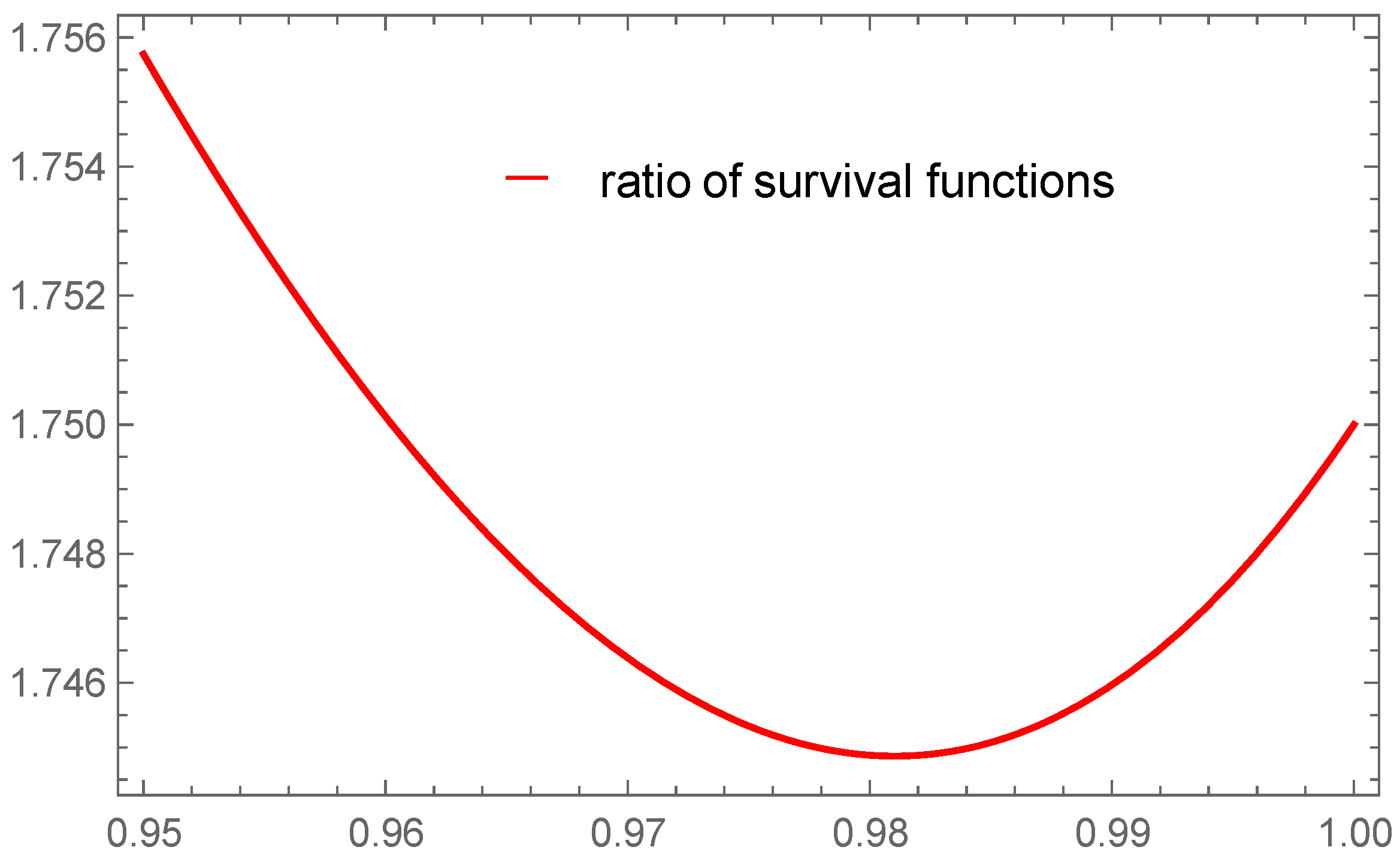
Example 1.
Let us consider as baseline distribution function. Set , and . Then, we find
to be not monotone when (as seen in Figure 1), and this negates the results that and .
Remark 1.
Under the , the result of Theorem 1 also hold under the following conditions:
- 1.
- and ;
- 2.
- and .
We now present an example to show that Part (ii) of Theorem 1 may not hold when .
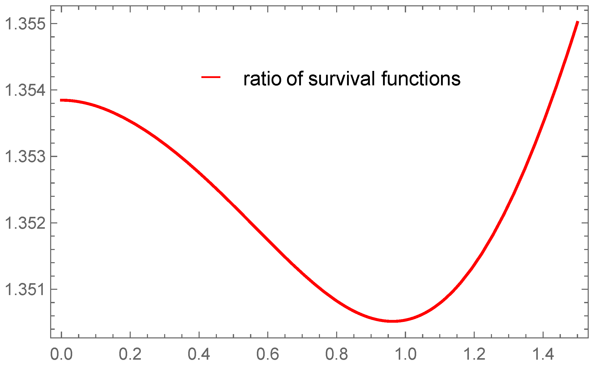
Example 2.
Let us consider the standard exponential as baseline distribution with , for . Set , and . Clearly, and . We then have
to be not monotone in (as seen in Figure 2), and this negates the results that and .
4. Reversed Hazard Rate Order
In this section, we discuss stochastic comparisons of parallel systems for different probabilities of starters in terms of reversed hazard rate order. For this purpose, we first prove the following lemma.
Lemma 3.
Suppose function is a differentiable function in x and
If we consider as
where denotes the derivative of function with respect to x, then:
Proof.
We can observe that
□
Theorem 2.
Suppose and are independent non-negative random variables with . Further, suppose , , , and are independent Bernoulli random variables, independently of s, with and , . Let and . Then, the following statements hold true:
- (i)
- If () and ( ), then
- (ii)
- If , then
Proof.
- (i)
- The distribution functions of and are given byFor the necessity part, from , we have , and sowhich implies thatThen, we havewhich implies that . Next, for the sufficiency part, let us consider the functionIt is then enough to show that is increasing in x. Upon differentiating with respect to x, we findHence, is increasing in x, which completes the proof of Part (i) of the theorem.
- (ii)
- The distribution functions of and , for , are given byandrespectively. Then, it is enough to show thatis increasing in x. Since and , there exist positive real numbers d and c such that and , and then we can rewrite as follows:Let us consider as follows:where . We can then see easily thatwhere andBecauseaccording to Lemma 3, we haveand clearly, for proving increasing property of with respect to x, it is enough to prove that the function is increasing in a and also in b. First, we havewhich shows that is increasing in a. Next, we also havewhich shows that is increasing in b. Now, since is increasing in a and , we haveFurther, since is increasing in b and (because ), we have
□
Remark 2.
The results of Theorem 2 also hold under the following conditions:
- 1.
- and ;
- 2.
- and .
5. Usual Stochastic Order
In this section, we present some stochastic comparisons of parallel systems for different components and different probabilities of starters in terms of the usual stochastic order.
Theorem 3.
Suppose () are independent non-negative random variables with (), . Further, suppose () are independent Bernoulli random variables, independently of s and s, with and , . Let and . If and , then .
Proof.
Let us denote . For , we can observe that . For obtaining the desired result, it is sufficient to observe that . Therefore, we have to check Conditions (i) and (ii) of Lemma 1. It is then evident that is symmetric with respect to , for any x. Additionally, for any , we have
Thus, we get
Hence, is Schur-convex with respect to , for any x. This implies that , as required. □
6. Concluding Remarks
A parallel system is one of the most commonly used coherent systems in practice. For this reason, a careful study of its performance characteristics, such as reliability function, hazard function and reversed hazard function, based on the characteristics of the component lifetime distribution, is of great interest to reliability engineers. In this work, we have focused our attention primarily on a parallel system with two components as a parallel system with more components can be decomposed into many subsystems with two components in parallel. One of the prominent examples of a two-component parallel system is a twin-engine jet system, which, in addition to being safer than a single-engine jet system, is more efficient in terms of fuel consumption than a jet system with more than two engines.
Specifically, we have proved the hazard rate and reversed hazard rate orders of parallel systems with two components having proportional hazard rates and starting devices.
It will be of interest to consider the problems discussed here by allowing dependence between components using some general copulas for the joint distribution of lifetime components. We are working in this direction at the present time and will present the corresponding results in the future.
Author Contributions
Conceptualization, G.B. and S.K.; Methodology, N.B., G.B. and S.K.; Software, S.K.; Validation, G.B. and S.K.; Formal analysis, N.B., G.B. and S.K.; Investigation, G.B. and S.K.; Resources, G.B.; Data curation, Not applicable; Writing —Original draft preparation, G.B.; Review and editing, N.B.; Visualization, G.B. and S.K.; Supervision, N.B.; Project administration, N.B. and G.B.; Funding acquisition, N.B. All authors have read and agreed to the published version of the manuscript.
Funding
This research received no external funding.
Institutional Review Board Statement
Not applicable.
Informed Consent Statement
Not applicable.
Data Availability Statement
Data sharing not applicable.
Acknowledgments
We express our sincere thanks to the Guest Editor and anonymous reviewers for their useful comments and suggestions on an earlier version of this manuscript that led to this improved version. This work has been conducted by University of Zabol, Grant Number: UOZ-GR-3389.
Conflicts of Interest
Data sharing not applicable.
References
- Fang, R.; Li, X. Advertising a second-price auction. J. Math. Econ. 2015, 61, 246–252. [Google Scholar] [CrossRef]
- Li, C.; Li, X. Stochastic comparisons of parallel and series systems of dependent components equipped with starting devices. Commun. Stat. Theory Methods 2019, 48, 694–708. [Google Scholar] [CrossRef]
- Li, X.; Zuo, M.J. Preservation of stochastic orders for random minima and maxima, with applications. Nav. Res. Logist. 2004, 51, 332–344. [Google Scholar] [CrossRef]
- Da, G.; Ding, W.; Li, X. On hazard rate ordering of parallel systems with two independent components. J. Stat. Plan. Inference 2010, 140, 2148–2154. [Google Scholar] [CrossRef]
- Joo, S.; Mi, J. Some properties of hazard rate functions of systems with two components. J. Stat. Plan. Inference 2010, 140, 444–453. [Google Scholar] [CrossRef]
- Di Crescenzo, A.; Di Gironimo, P. Stochastic comparisons and dynamic information of random lifetimes in a replacement model. Mathematics 2018, 6, 204. [Google Scholar] [CrossRef] [Green Version]
- Barmalzan, G.; Payandeh Najafabadi, A.T.; Balakrishnan, N. Ordering properties of the smallest and largest claim amounts in a general scale model. Scand. Actuar. J. 2017, 2017, 105–124. [Google Scholar] [CrossRef]
- Zhang, Y.; Cai, X.; Zhao, P. Ordering properties of extreme claim amounts from heterogeneous portfolios. ASTIN Bull. 2019, 49, 525–554. [Google Scholar] [CrossRef]
- Marshall, A.W.; Olkin, I. Life Distributions; Springer: New York, NY, USA, 2007. [Google Scholar]
- Müller, A.; Stoyan, D. Comparison Methods for Stochastic Models and Risks; John Wiley & Sons: New York, NY, USA, 2002. [Google Scholar]
- Shaked, M.; Shanthikumar, J.G. Stochastic Orders; Springer: New York, NY, USA, 2007. [Google Scholar]
- Marshall, A.W.; Olkin, I.; Arnold, B.C. Inequalities: Theory of Majorization and Its Applications, 2nd ed.; Springer: New York, NY, USA, 2011. [Google Scholar]
Figure 1.
Plot of the ratio of survival functions of and for in Example 1.

Figure 2.
Plot of the ratio of survival functions of and for in Example 2.

Publisher’s Note: MDPI stays neutral with regard to jurisdictional claims in published maps and institutional affiliations. |
© 2021 by the authors. Licensee MDPI, Basel, Switzerland. This article is an open access article distributed under the terms and conditions of the Creative Commons Attribution (CC BY) license (https://creativecommons.org/licenses/by/4.0/).
Share and Cite
MDPI and ACS Style
Balakrishnan, N.; Barmalzan, G.; Kosari, S. Comparisons of Parallel Systems with Components Having Proportional Reversed Hazard Rates and Starting Devices. Mathematics 2021, 9, 856. https://0-doi-org.brum.beds.ac.uk/10.3390/math9080856
AMA Style
Balakrishnan N, Barmalzan G, Kosari S. Comparisons of Parallel Systems with Components Having Proportional Reversed Hazard Rates and Starting Devices. Mathematics. 2021; 9(8):856. https://0-doi-org.brum.beds.ac.uk/10.3390/math9080856
Chicago/Turabian StyleBalakrishnan, Narayanaswamy, Ghobad Barmalzan, and Sajad Kosari. 2021. "Comparisons of Parallel Systems with Components Having Proportional Reversed Hazard Rates and Starting Devices" Mathematics 9, no. 8: 856. https://0-doi-org.brum.beds.ac.uk/10.3390/math9080856
Note that from the first issue of 2016, this journal uses article numbers instead of page numbers. See further details here.