
Direct Collocation with Reproducing Kernel Approximation for Two-Phase Coupling System in a Porous Enclosure


1
Department of Civil Engineering, National Yang Ming Chiao Tung University, Hsinchu 30010, Taiwan
2
Department of Civil Engineering, National Chiao Tung University, Hsinchu 30010, Taiwan
*
Author to whom correspondence should be addressed.
Mathematics 2021, 9(8), 897; https://doi.org/10.3390/math9080897
Submission received: 1 April 2021
/
Revised: 14 April 2021
/
Accepted: 16 April 2021
/
Published: 17 April 2021
(This article belongs to the Special Issue Analytical and Numerical Methods for Linear and Nonlinear Analysis of Structures at Macro, Micro and Nano Scale)
Abstract
:The direct strong-form collocation method with reproducing kernel approximation is introduced to efficiently and effectively solve the natural convection problem within a parallelogrammic enclosure. As the convection behavior in the fluid-saturated porous media involves phase coupling, the resulting system is highly nonlinear in nature. To this end, the local approximation is adopted in conjunction with Newton–Raphson method. Nevertheless, to unveil the performance of the method in the nonlinear analysis, only single thermal natural convection is of major concern herein. A unit square is designated as the model problem to investigate the parameters in the system related to the convergence; several benchmark problems are used to verify the accuracy of the approximation, in which the stability of the method is demonstrated by considering various initial conditions, disturbance of discretization, inclination, aspect ratio, and reproducing kernel support size. It is shown that a larger support size can be flexible in approximating highly irregular discretized problems. The derivation of explicit operators with two-phase variables in solving the nonlinear system using the direct collocation is carried out in detail.
1. Introduction
In the literature, there is a bunch of numerical studies on double-diffusive natural convection in enclosures filled with fluid-saturated porous media [1]. It was not until the investigation by Costa that the enclosure of a parallelogram was numerically and theoretically studied in detail [2]. In the practical application, a parallelogrammic enclosure is referred to as the diode of heat and mass transfer owing to the fact that its inclined angle, aspect ratio, and boundary conditions can be designed to meet different purposes concerning various heat and mass transfer characteristics. Nevertheless, the coupling feature of three variables, including temperature, stream function, and concentration, in the problem of double-diffusive natural convection in a parallelogrammic porous enclosure inevitably leads to a highly nonlinear system of partial differential equations (PDEs).
Among the numerical methods for solving PDEs governed by diffusion-convection in parallelogrammic enclosures, the mesh-based methods were adopted early, while the meshfree methods were introduced in recent years. For instance, the finite difference method was employed in the analysis of double-diffusive convection in a porous enclosure with a rectangular shape in 2002 [3]. Around the same time, the finite element method was used to solve the two-dimensional double-diffusive natural convection problem [2]. With the prosperous development of numerical methods in computational mechanics, there was a tendency towards boundary-type methods, in addition to the domain-type methods. To name but a few, the boundary domain integral method was applied to study the double diffusive natural convection in porous media [4]; the boundary element method was introduced to simulate three-dimensional double-diffusive natural convection in porous media [5]. As the meshfree methods get rid of mesh constraint and the strong form methods discard domain integral, a growing number of studies appear and are reported as follows: the local radial basis collocation method was used to solve the two-dimensional double diffusion and natural convection problem in 2012 [6]; the exponentially convergent scalar homotopy algorithm was introduced as the nonlinear solver. Later, in 2018, the generalized finite difference method combined with the Newton–Raphson method was proposed to solve both single thermal natural convection in parallelogrammic enclosures and double-diffusive natural convection in parallelogrammic enclosures filled with fluid-saturated porous media [7].
By examining the work done by Fan et al. [6] and Li et al. [7], the major features in common is the local approximation adopted in the meshfree methods, in which a stable system of equations can be established for nonlinear analysis. As motivated by this idea, the present study proposes the reproducing kernel collocation method in conjunction with the Newton–Raphson method to efficiently and effectively solve the natural convection problems with parallelogrammic enclosures. As there exist several parameters affecting the convergence of the proposed method in solving nonlinear PDEs, only single thermal natural convection in parallelogrammic enclosures filled with fluid-saturated porous media is considered in this study.
In the collocation methods, both global and local functions can be used in the approximation. The commonly adopted global function is the radial basis function (RBF) defined by the Euclidean norm; nevertheless, the shape parameter of RBF cannot be determined uniquely by a given formula so far. As the resulting system is often ill-conditioned with a large condition number, numerical instability might be raised; for more information, see [8,9,10]. In contrast, the reproducing kernel (RK) shape function is a local function; although it maintains an algebraic convergence rate, the resulting system is more stable to yield promising results [11,12,13]. Other types of approximation adopted in the collocation method, such as global expansion in Bernstein polynomials, exponential functions, and Taylor matrix, can be referred to the studies [14,15,16] for solving nonlinear ODE systems. Regarding the two-phase coupling problems, the concept of u-p formulation for describing displacement–pressure behavior was developed early in the Biot theory for the analysis of poromechanics in fluid-saturated media [17]. Later, the u-p formulation was further introduced in the weak-form reproducing kernel particle method (RKPM) to perform the hydro-mechanical analysis in porous media coupled by solid stiffness matrix and compressibility matrix [18]. Unlike the u-p formulation for describing displacement and pressure, the present study first introduces the strong-form reproducing kernel collocation method (RKCM) to the analysis of two-phase coupling system governed by thermal-convection equations.
The structure of this study is the following: the mathematical formulation of the two-phase coupling in a porous enclosure is re-visited in Section 2. The RKCM for the nonlinear system coupled by two variables is introduced with detailed formulation in direct collocation in Section 3. Four numerical examples are given in Section 4. Section 5 concludes the present study.
2. Mathematical Formulation
2.1. Governing Equations
As shown in Figure 1a, the parallelogram is formed by an angle with two sides of length and . Assuming that the fluid-saturated porous medium has two phases, the components of flux or velocity and along the and directions are described by Darcy’s law with the following proportionality to pressure drop:
where is the permeability of the isotropic medium; , , and are the dynamic viscosity, pressure, and density of the fluid, respectively; and is the gravitational constant. The stream function is introduced to relate the flux as given by:
For the sake of convenience, Equations (1) and (2) are normalized as:
where the non-dimensional parameters , , and are used. is the thermal diffusivity of the porous medium; nevertheless, it is assumed to be the thermal diffusivity of the fluid alone herein, i.e., the effective thermal diffusivity [1,2]. The non-dimensional temperature is given by:
where the subscript in Equation (7) represents the quantity in the physical domain; the subscripts and refer to the corresponding higher and lower values. For the non-solute transferring problem, the governing equations are described by the balance laws of linear momentum and thermal energy:
where a steady state is assumed in the above two equations. Introducing Equations (5) and (6) to Equation (9) gives:
For natural heat convection in a non-porous medium, Rayleigh number and Darcy number are:
where is the thermal expansion coefficient () and is the kinematic viscosity of the fluid. Based on Equations (11) and (12), the Darcy-modified Rayleigh number can be defined as:
which is also the non-dimensional parameter.
2.2. Boundary Conditions
Referring to the general model depicted in Figure 1b, the boundary walls of the porous medium in a parallelogram are assumed to be impermeable, which indicates . As such, the non-dimensional components of velocity and are zero at boundary walls, while they can be evaluated by using Equations (5) and (6). The explicit boundary conditions for and together with are described as follows:
Along the inclined bottom side:
Along the inclined upper side:
In Equations (16) and (17), denotes the non-dimensional normal to the inclined wall.
3. RKCM for a Nonlinear Coupling System
3.1. Reproducing Kernel Approximation for Two-Phase Variables
To efficiently solve the nonlinear system of equations, the RK shape functions are introduced for two variables and at source points as follows:
where and are the generalized coefficients. is the RK shape function consisting of a monomial basis , coefficient vector , and kernel function of the following form:
where is found by the reproducing conditions listed below:
where is the multi-index defined as , and is the order of . The detailed derivation of RK shape functions is referred to previous work [19]. The explicit form of RK shape functions is:
with the moment matrix given by:
To ensure continuity, the high order B-spline kernel function is usually required in strong form collocation methods. The quintic B-spline kernel function used herein is given by:
where the normalized nodal distance , and a denotes the radius of a circular support. For the th order monomial basis, the RK support size is chosen to be proportional to the average nodal distance , i.e., with for any discretization.
The two equations in Equation (18) can be combined as:
with:
Substituting Equation (24) into Equations (8) and (10) leads to:
Similarly, substituting Equation (24) into Equations (14)–(17) gives the following equations:
along , and:
along , and:
for the inclined bottom side, and:
for the inclined upper side.
3.2. Newton–Raphson Collocation Method for Nonlinear System
From Equations (28) and (29), it is obvious that the system is nonlinear and coupled by two phases. To this end, the Newton–Raphson method is introduced under the collocation framework, which is designated as a Newton–Raphson collocation method in this work.
As a beginning of the formulation, three sets of collocation points are defined: for governing equations in the domain, for Neumann boundary conditions, and for Dirichlet boundary conditions. Note that the same discretization of collocation points and source points is adopted herein; for two field variables, the total number of collocation equations is , which is equal to . By using the direct collocation, Equations (28)–(33) can be recast as follows:
where:
with:
Nevertheless, to obtain the general expression of boundary collocation equations for wider application, the prescribed non-zero values, but not limited to, of both Neumann and Dirichlet boundary conditions are presented. That is, , , , and are assumed in the following derivation. Therefore:
As the collocation system is coupled in matrix , the nonlinear version of direct collocation is established by using the Newton–Raphson method given by:
in which the superscript denotes the step of iteration and is the Jacobian matrix defined as . Thus, the Jacobian matrix is derived as:
in which:
with:
and:
However, from Equation (40), it can be observed that the computation of the inverse of the Jacobian matrix at each iteration is computationally expansive. As such, the following two-step Newton–Raphson method is adopted [7]:
where denotes the increment of vector at th step. The explicit expressions for matrices and are detailed in Appendix A. The stopping criterion for iteration is given by:
which is adopted in the present study.
3.3. Remarks
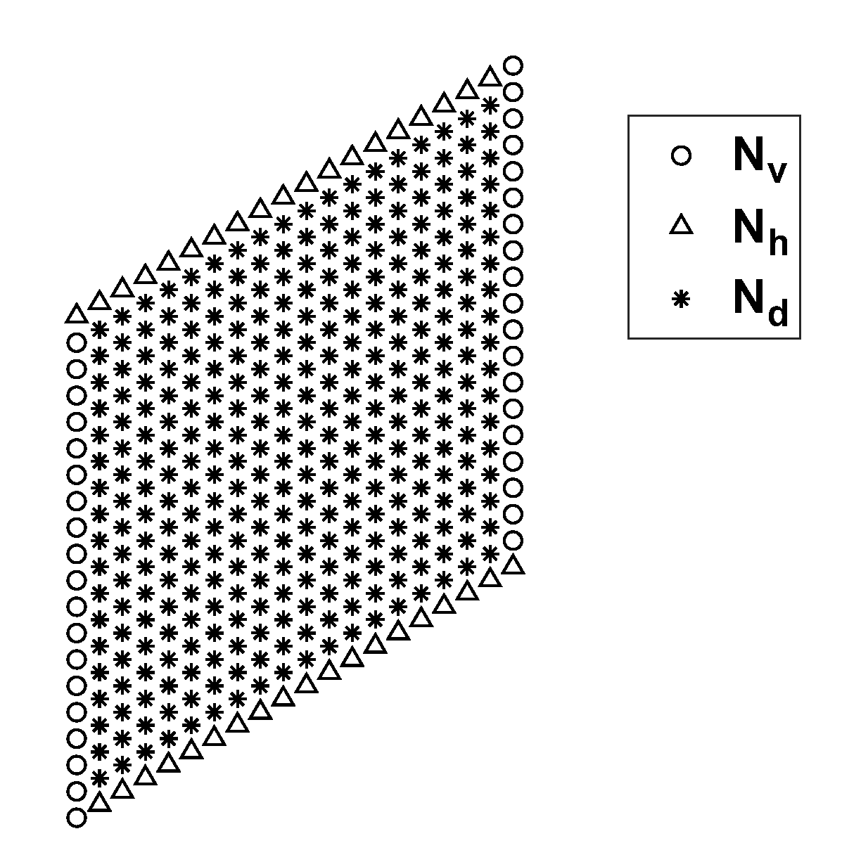
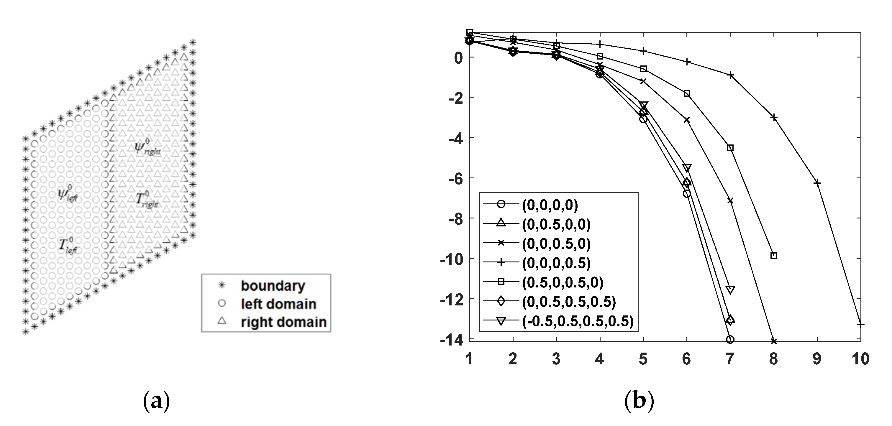
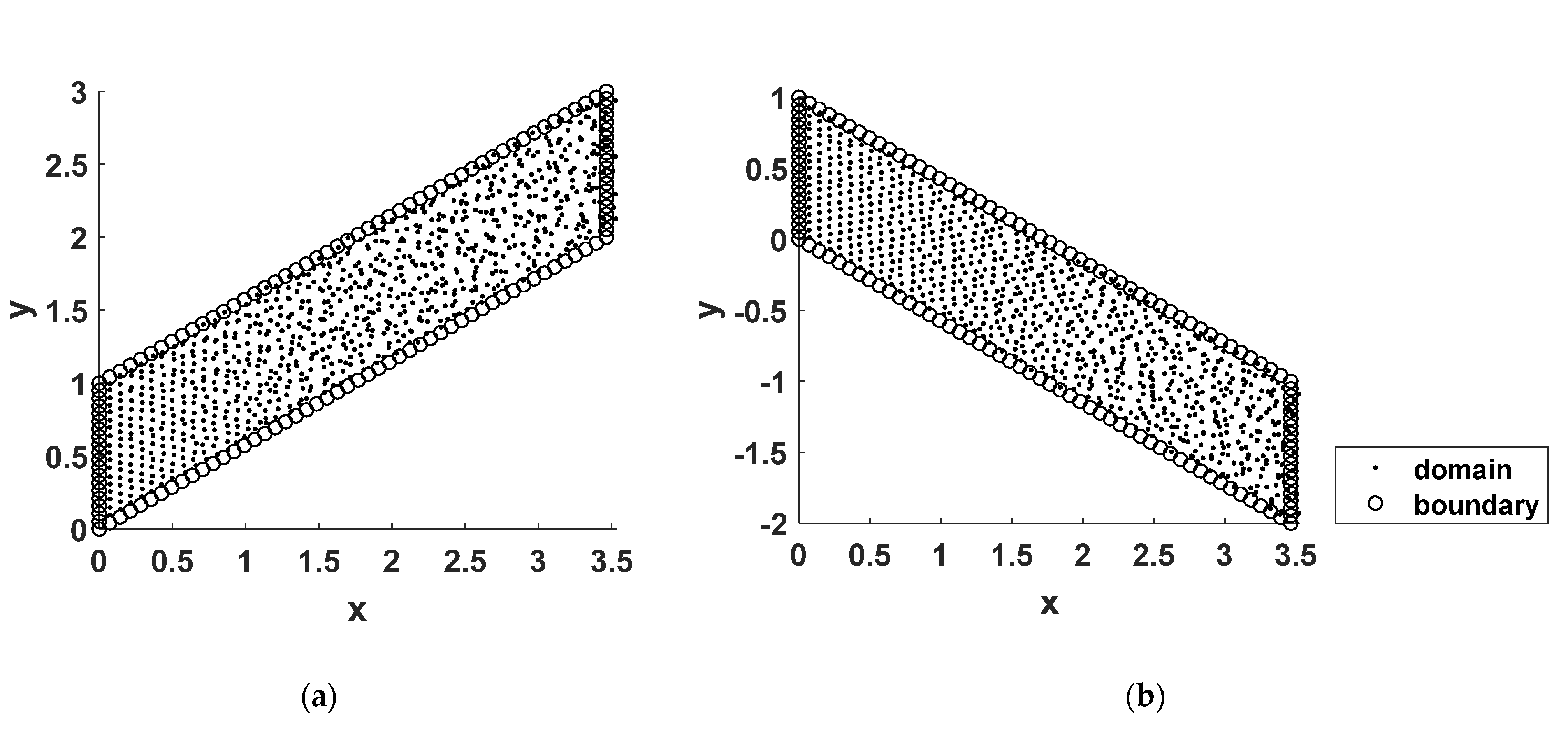
For illustration purpose, a schematic diagram of discretization shown in Figure 2 is considered, where the numbers of collocation points in the parallelogram are marked by , , and for vertical, inclined, and domain points, respectively. It is noted that the four corner points are included in the present method without causing any difficulty in the numerical simulation, while they were excluded in the generalized finite difference method as reported in [7].
By taking the boundary conditions described in Equations (14)–(17) or Equations (30)–(33) as an example, the total collocation points are with , , and . This indicates that the Jacobian matrix is a square matrix, and the resulting system is determined. As such, the present study adopts the direct collocation method. For the problem in consideration, the same location and number of source points and collocation points are utilized herein, i.e., Ns = Nc. Unlike the weighted collocation method with least-squares formulation in the previous studies [11,12,13,19], there are typically more collocation points than source points in the collocation system, and boundary conditions are imposed by weights to balance the errors in the domain and on the boundary. With the RK approximation in the direct collocation method, a sparse system of Jacobian matrix is reached, thereby making the Newton–Raphson collocation method efficient.
4. Numerical Examples
To validate the proposed method in solving the nonlinear system coupled by two-field variables, four numerical examples with various parallelogrammic geometries are provided in the following study. In the reproducing kernel collocation method, the RK shape functions are constructed by using the quadratic basis with a quintic B-spline kernel function, and the support size of RK shape functions is chosen as without loss of generality. In particular, the parametric study is conducted in each example to thoroughly understand the effect of nonlinearity and the convergence of approximation.
4.1. Square Domain
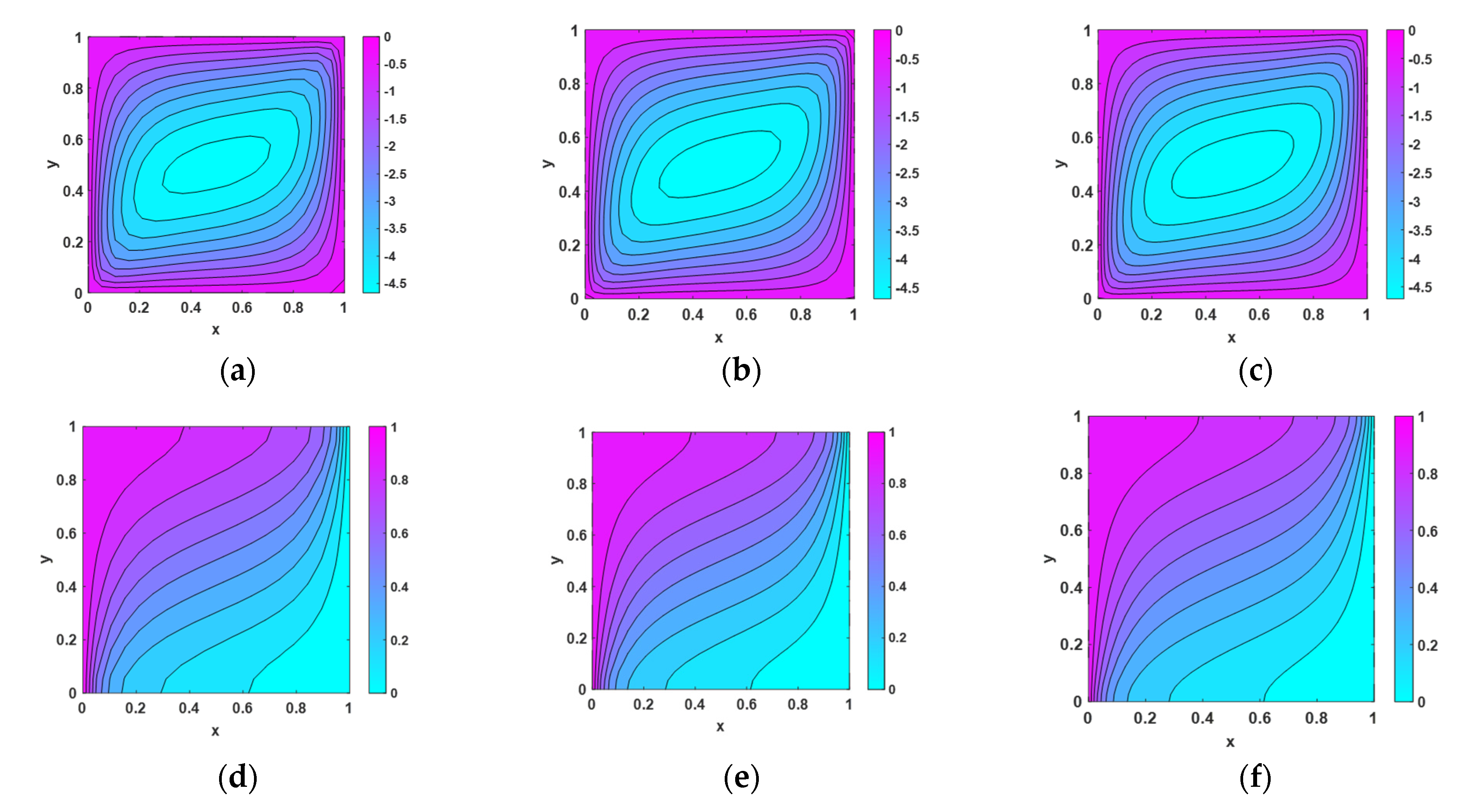
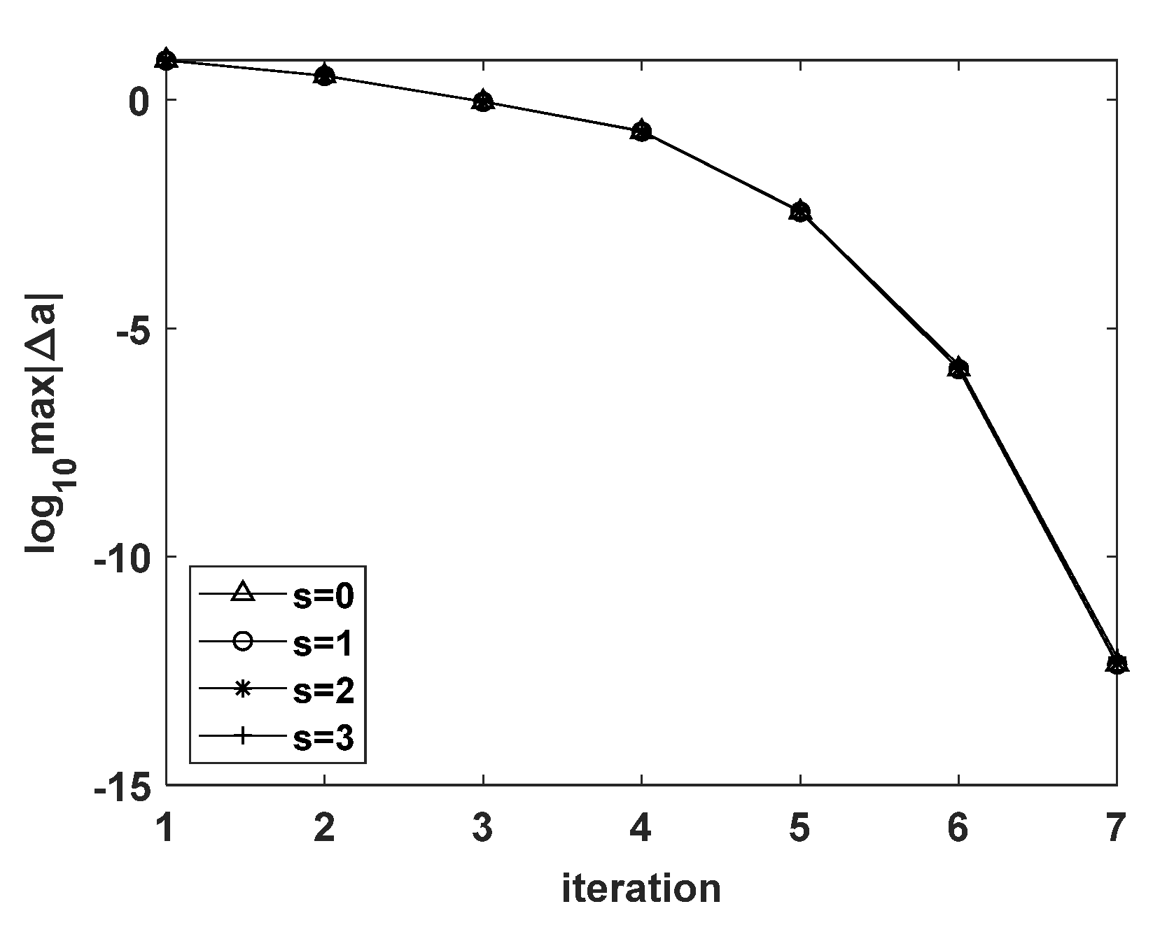
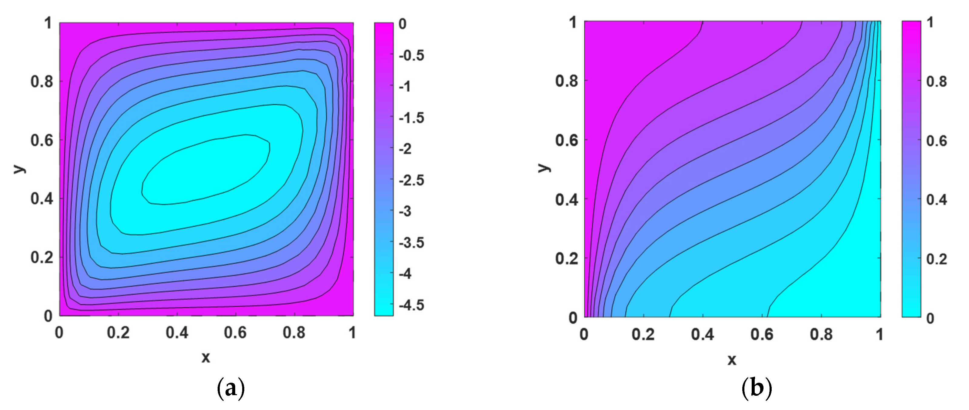
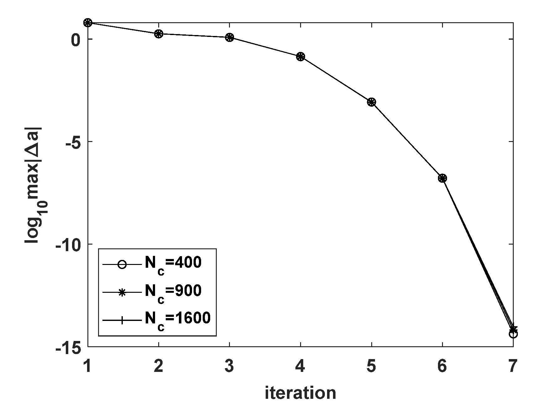
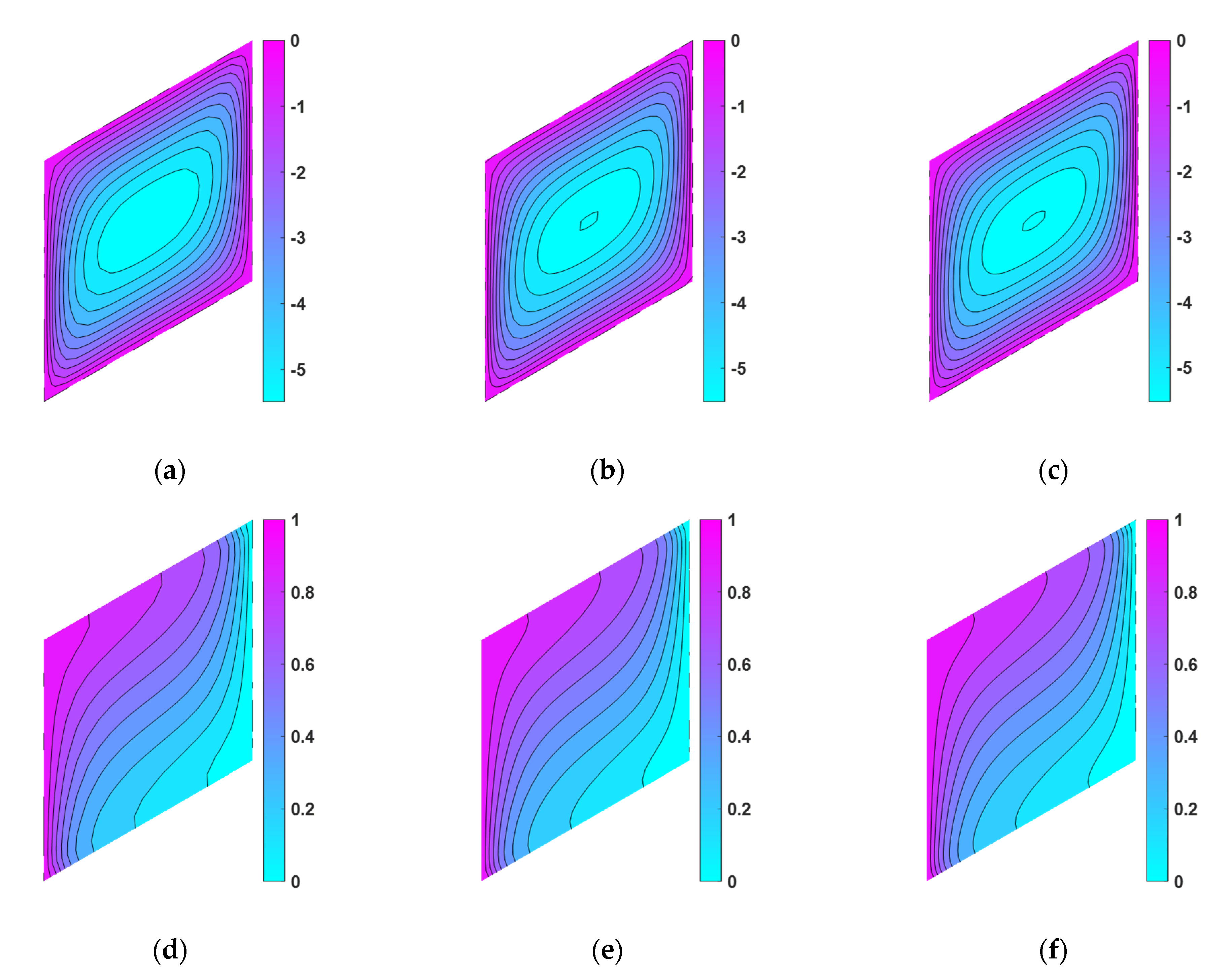
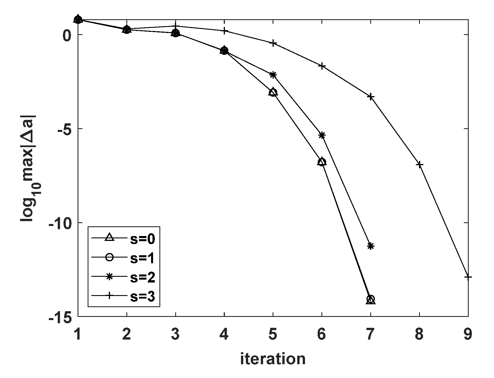
The schematic diagrams of the uniform and non-uniform discretizations in a unit square are depicted in Figure 3a,b, respectively. In the uniform discretization, three refinements with are considered in the approximation for with initial conditions . Figure 4 compares the number of iterations obtained by three refinements; Figure 5 shows the corresponding contour plots of and . Clearly, the present method converges fast and stably in 7 iterative steps for all discretizations; the contour plots of both and also exhibit the same pattern. The convergence of approximation is validated through the refinement of discretization. In the following study, is used. In Figure 3b, the non-uniformly discretized domain is obtained by adding 3% (disturbing factor ) disturbance to Figure 3a. By using the same values of and , the number of iterations for various non-uniform discretizations obtained by are given in Figure 6. For , the contour plots of and are shown in Figure 7, where a similar distribution of and to those obtained by uniform discretization is observed.
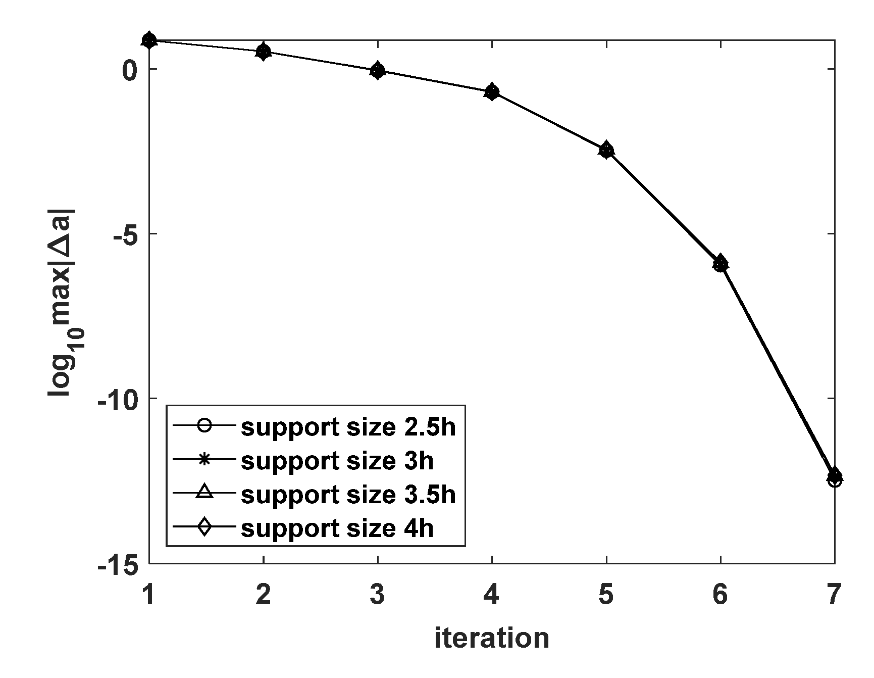
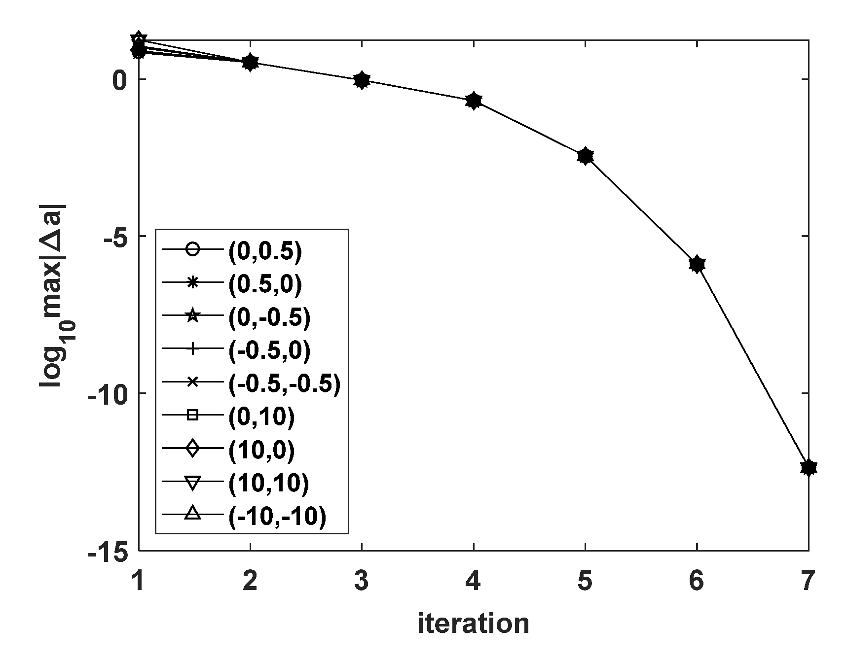
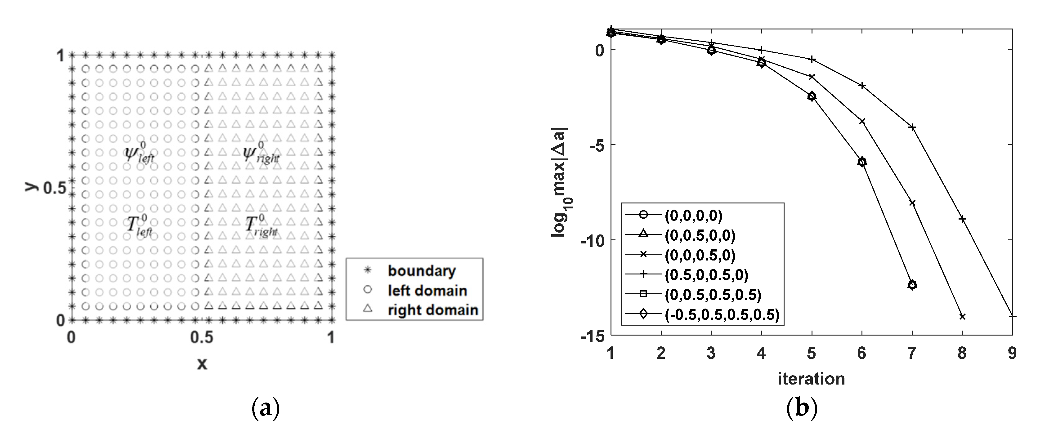
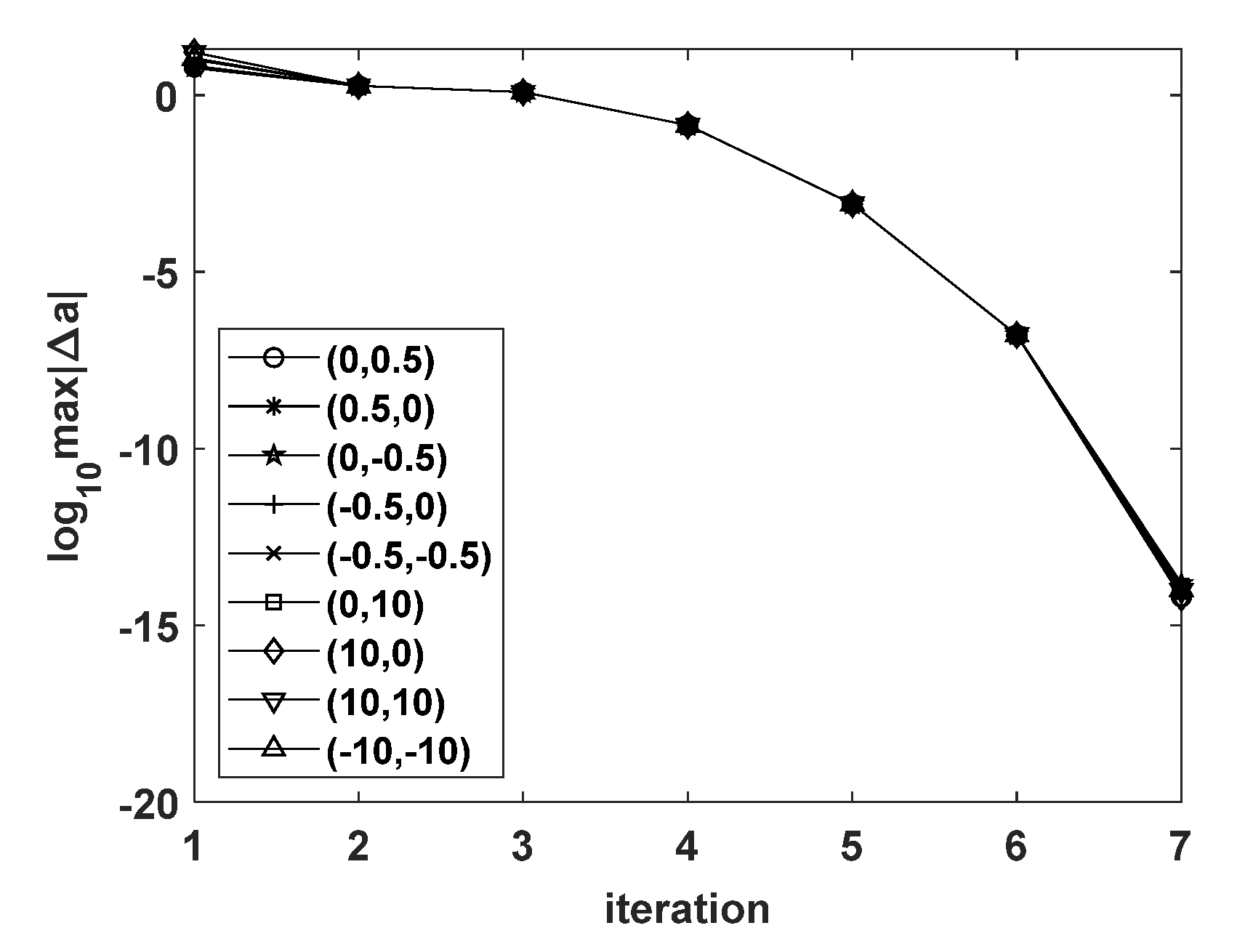
Based on the quadratic basis adopted in constructing the RK shape functions, the RK support size generally ranges from to . To understand the influence of support size for the nonlinear system, the number of iterations corresponding to various support size is summarized in Figure 8 for with . It is shown that the number of iterations is 7 for all cases regardless of the support size. As for the Newton–Raphson method, the choice of initial conditions may affect the convergence of approximation. To this end, several sets of initial conditions are tested, and the corresponding iteration is shown in Figure 9; all approximate solutions converge within 7 iterative steps, although their initial errors in the first step may be quite different. For wider application, various initial values, such as , are considered as depicted in Figure 10a; the corresponding iteration is shown in Figure 10b. It is found that the initial conditions might affect the path of convergence, and more iterations might be needed to meet the stopping criterion. Nevertheless, most initial conditions yield convergent approximation.
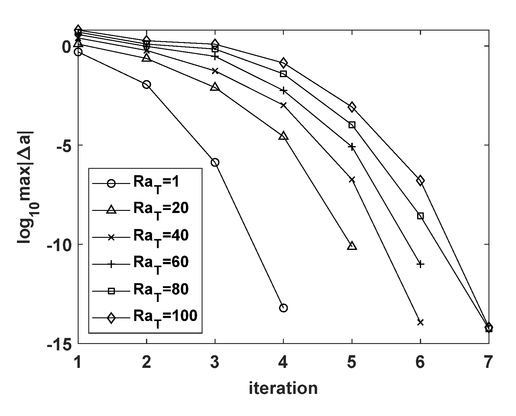
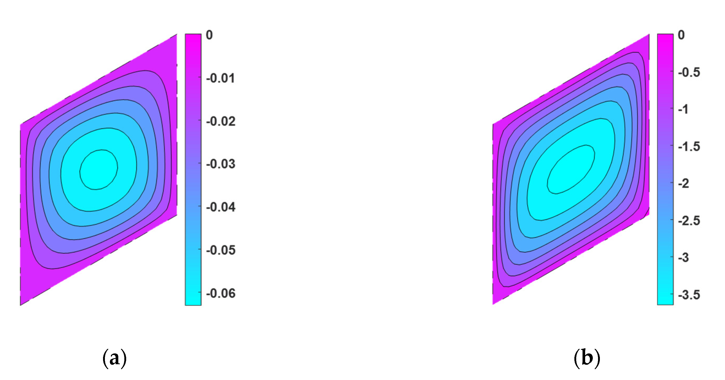
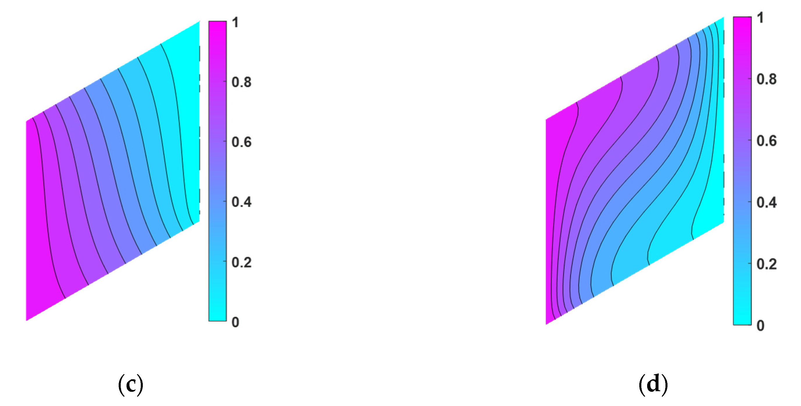
For the nonlinear system in consideration, the parameter governs the nonlinearity, and various values of such as 1 and 60 are considered herein. The comparison of the number of iterations obtained by various is made in Figure 11; it was found that more iteration steps are needed for a larger value of . For illustration purpose, the contour plots of and obtained by and are presented in Figure 12. From Figure 12a, the contour of is almost symmetric in both vertical and horizontal directions for ; as increases to 60 and 100, the contours of gradually showed anti-symmetric distribution along the line inclined at to the horizontal direction as referred to Figure 5b and Figure 12b. As for the contour of , with increasing , its distribution moved from a vertical direction toward a curved orientation as shown in Figure 5e and Figure 12c,d.
4.2. Diamond Domain
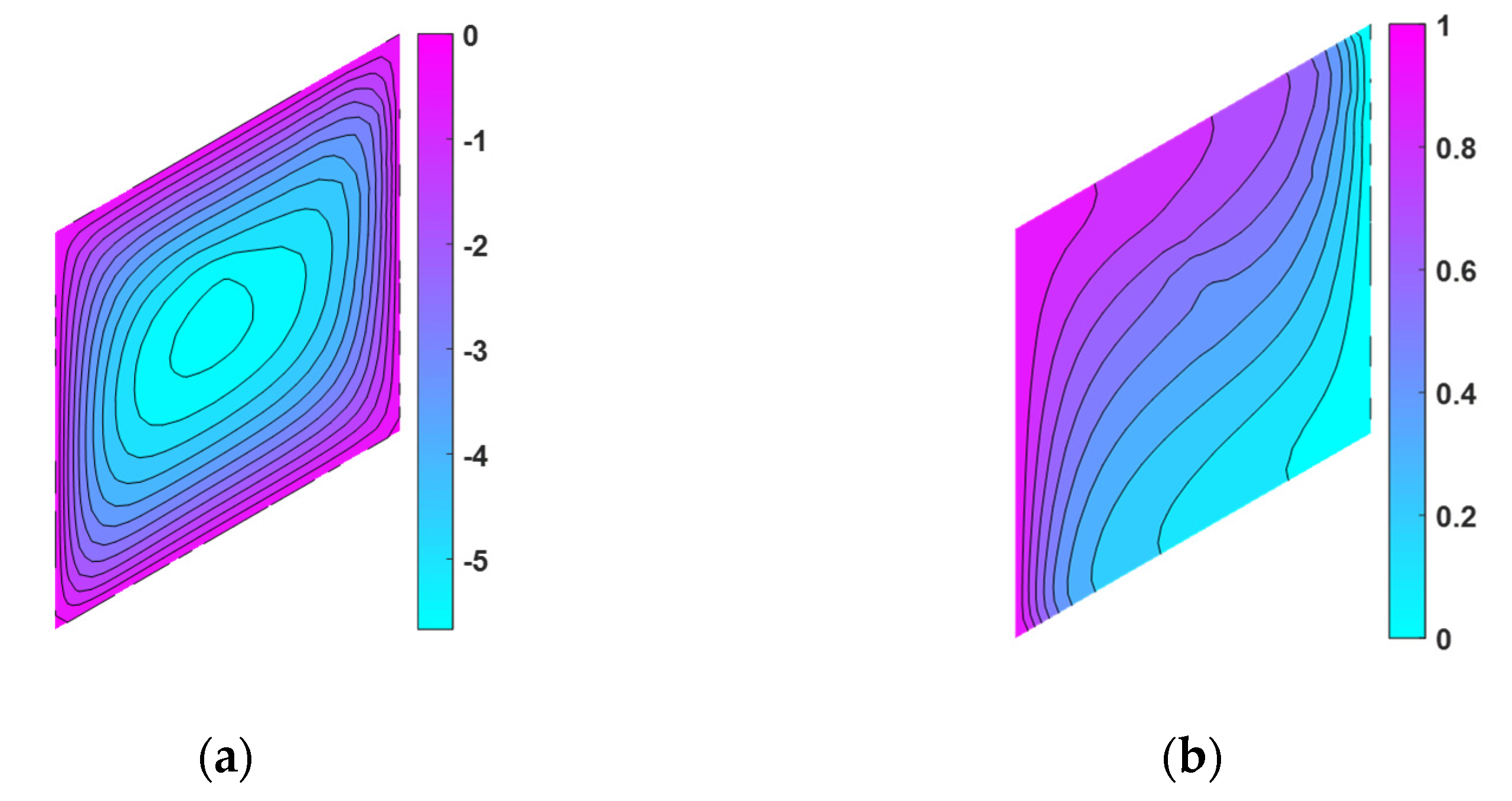
A unit diamond with is discretized uniformly and non-uniformly as shown in the schematic diagrams Figure 13a,b, respectively. The analysis is performed by following the previous example as described in Section 4.1. For and , the number of iterations obtained by uniform discretizations with are shown in Figure 14; the corresponding contour plots of and are given in Figure 15. It is shown that only 7 steps are required in the iteration process. In addition, the convergence of approximation is assured by the presence of consistent patterns in the contours, as also shown in the previous work [7]. The non-uniform discretization with in Figure 13b is obtained by adding 3% disturbance to the uniform discretization. For various percentage of disturbance , the number of iterations are given in Figure 16. For large disturbance , more iterations are required due to a longer path of convergence; the corresponding contour plots of and are shown in Figure 17, where similar patterns of and to those obtained by uniform discretization are retrieved, while the smoothness of the contours is reduced.
The influence of initial conditions are investigated by considering for entire domain and for two half domains, and the corresponding results are shown in Figure 18 and Figure 19, with Figure 19a illustrating the arrangement of . From Figure 18 and Figure 19b, it is observed that the initial conditions may affect the path of convergence, i.e., the number of iterations. As for the influence of , Figure 20 compares the number of iterations obtained by various ranging from 1 to 100; the larger value is, the more iterations it requires. The selected contour plots of and obtained by and are shown in Figure 21. As increases, the contour of changes from symmetry to anti-symmetry with respect to the line inclined at in the horizontal direction, and its magnitude increases as well, as shown in Figure 15b and Figure 21a,b. The contour of gradually changes the orientation from left to right with increasing nonlinearity, as can be observed in Figure 15e and Figure 21c,d.
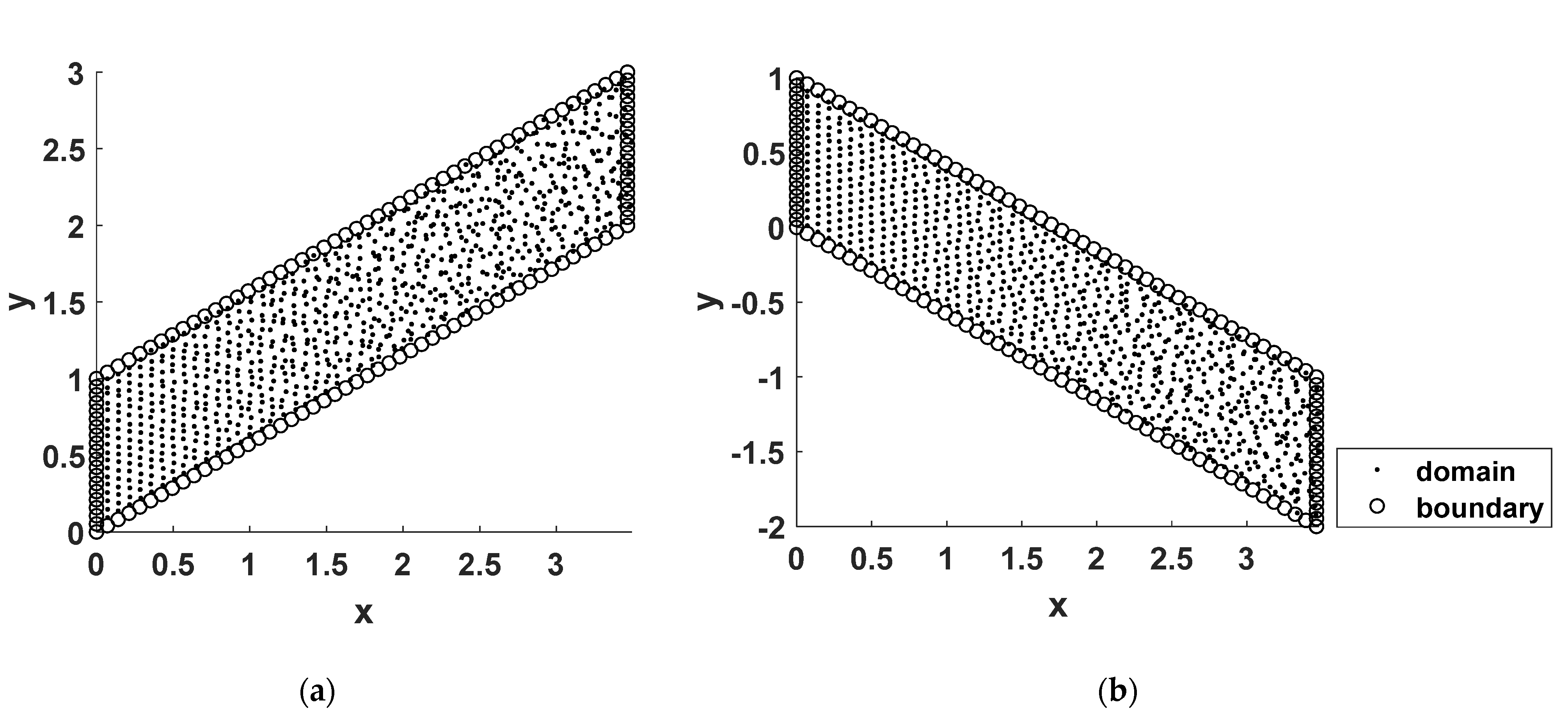
4.3. Parallelogram Domains I and II
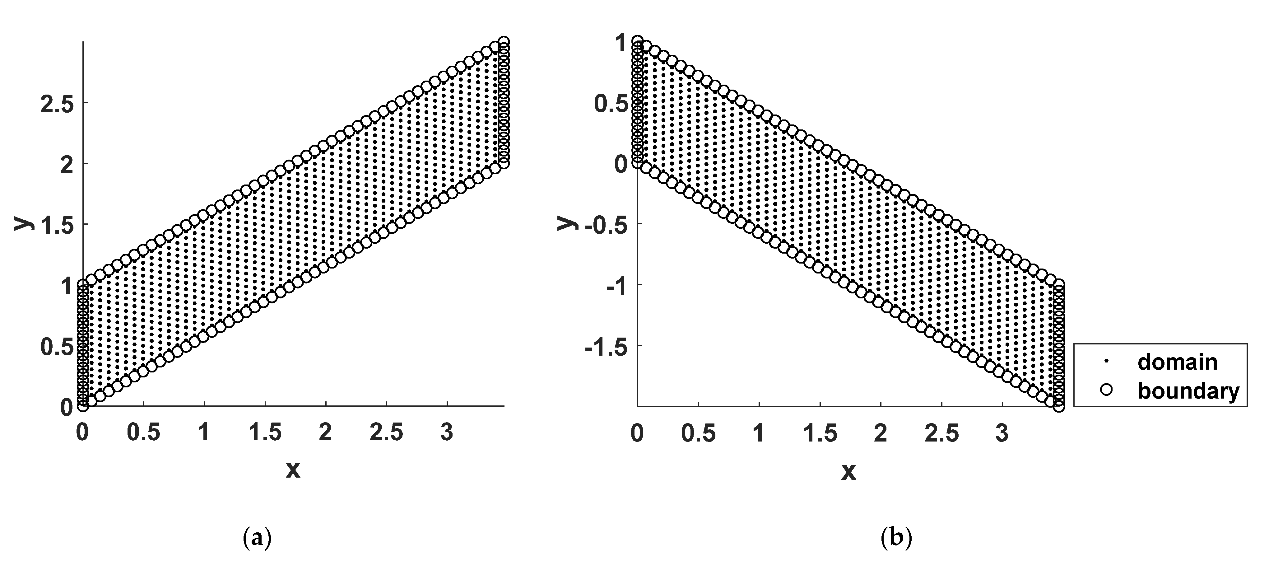
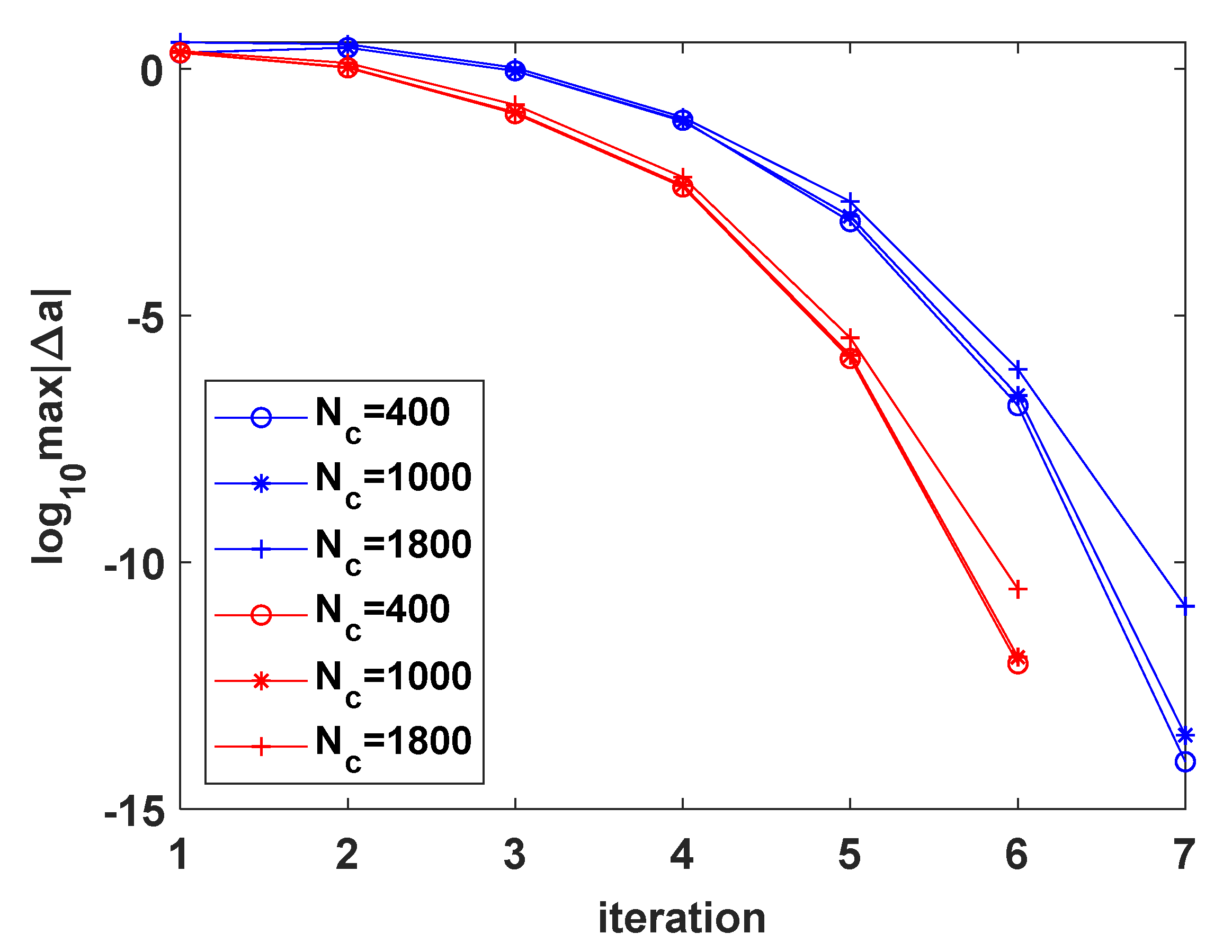
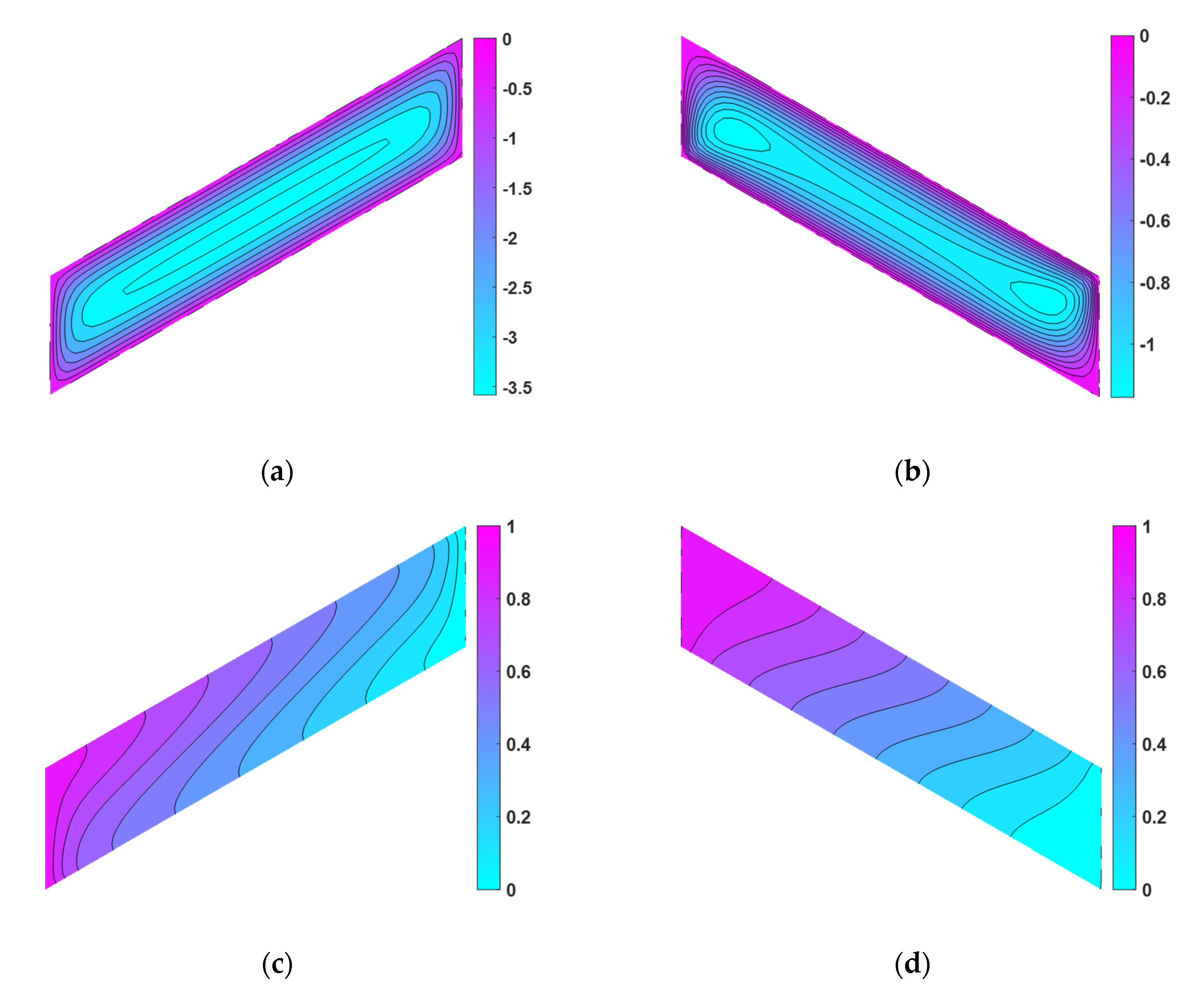
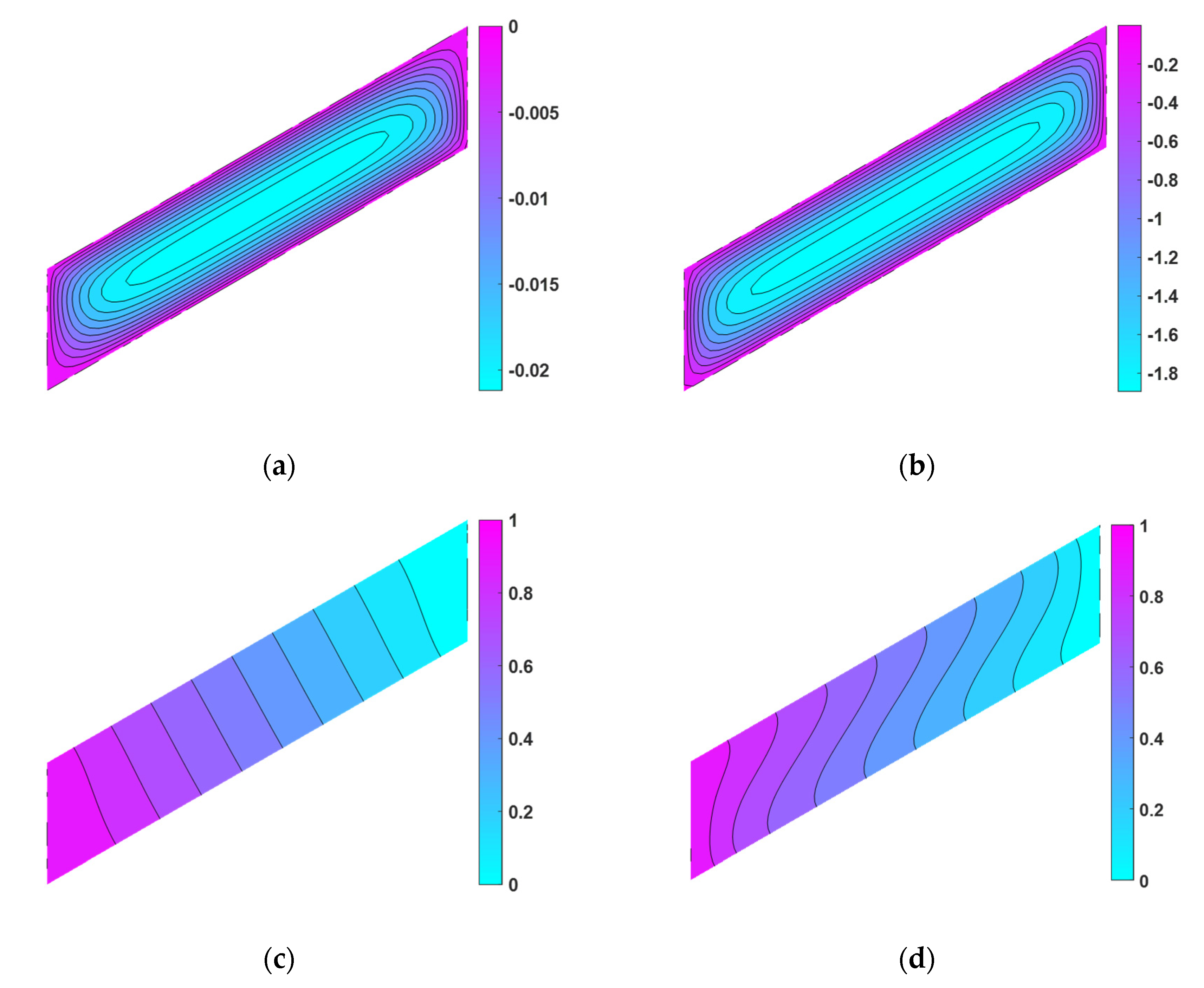
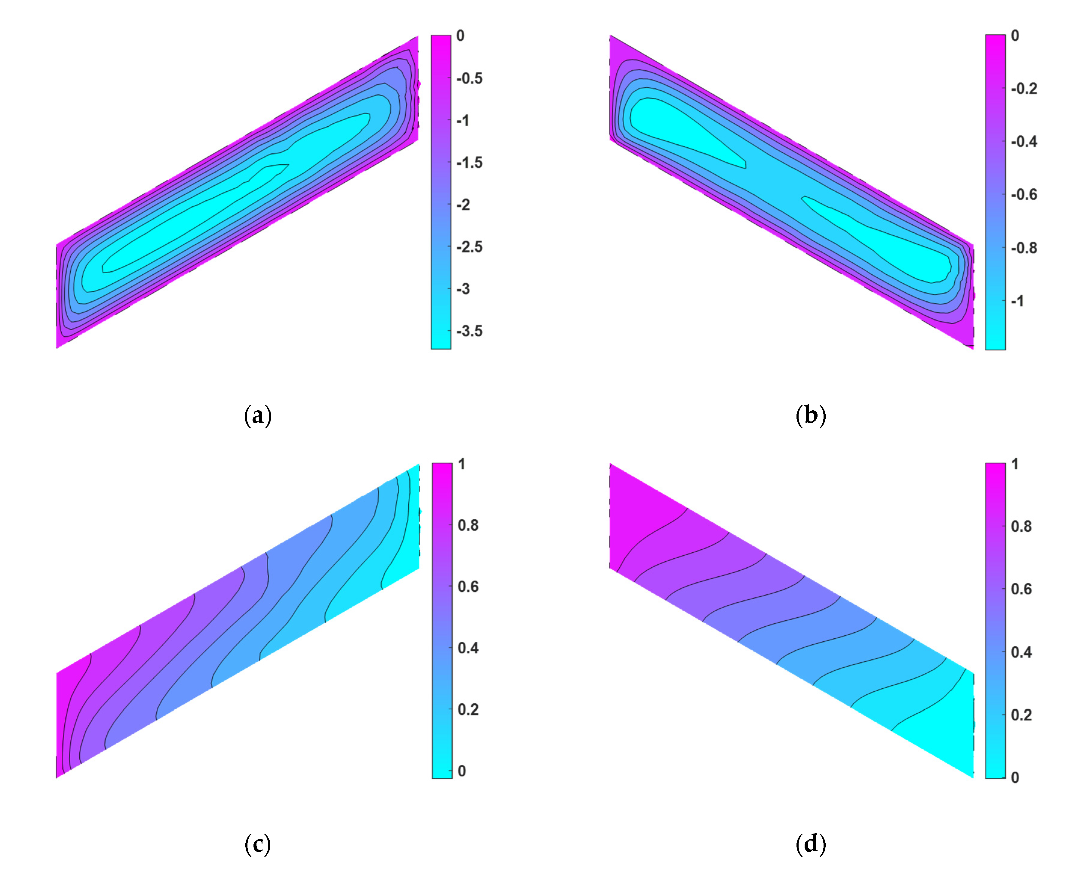
As shown in Figure 22a,b, two parallelograms () with inclined angles and are considered, in which the former is denoted as domain I, while the latter is denoted as domain II. For clarity, when comparing the results of two parallelograms in domain I and domain II, the corresponding results are depicted in terms of blue and red lines as will be shown in the following figures. For and , three refinements of uniform discretization with are considered. The path of convergence expressed in terms of iteration is depicted in Figure 23. In each domain, the approximation converges with the same number of iterations regardless of whether different points are used in the discretization; moreover, domain I shows slower convergence than domain II. The contour plots of and obtained by are shown in Figure 24, which are consistent with the results given in [7]. The distributions of both and in two domains are dissimilar due to different inclination; in particular, the contour of in domain II with a negative inclined angle has two small vortices at the two ends.
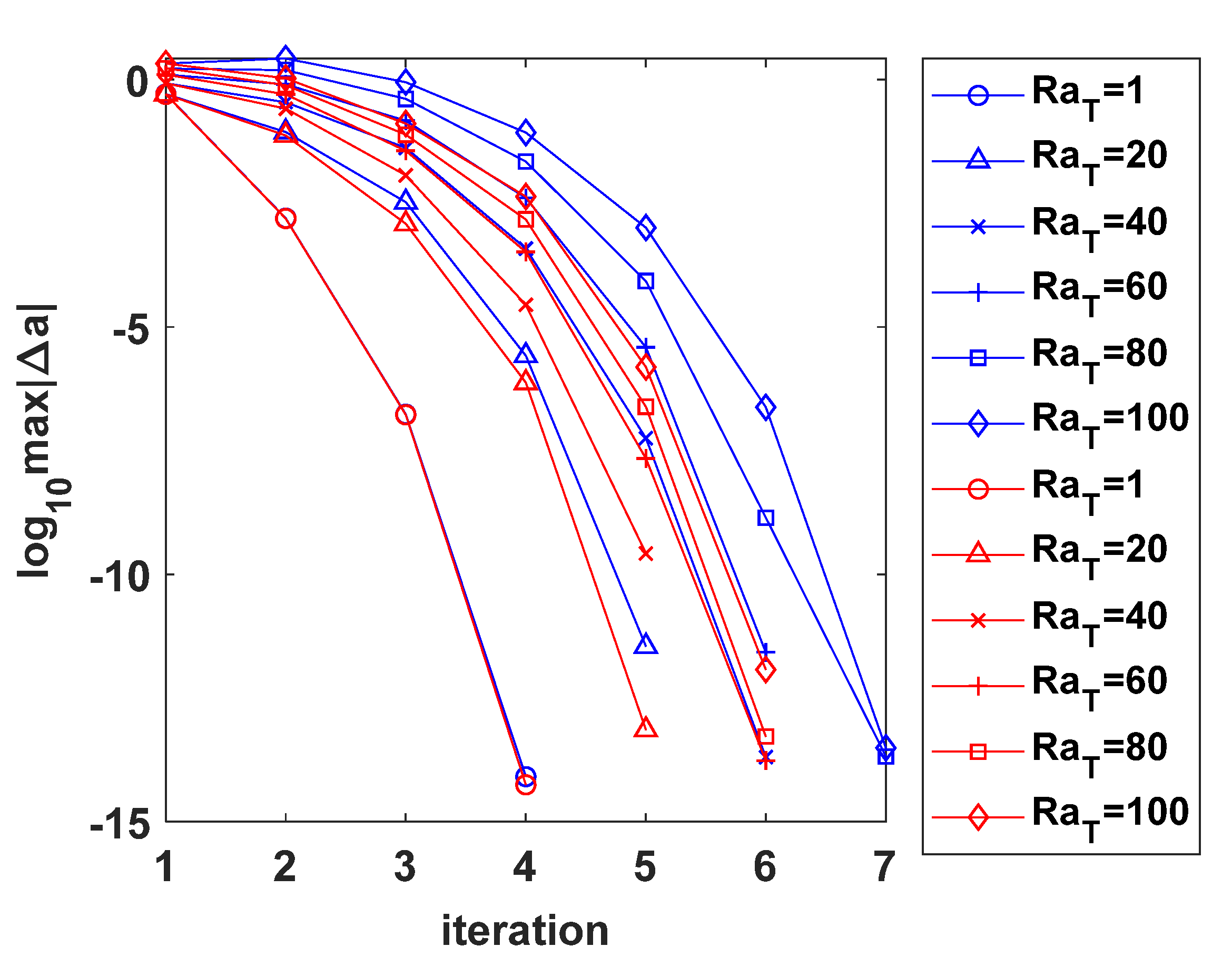
The influence of initial conditions on the solutions is investigated by concerning and for and ; the corresponding paths of iteration are shown in Figure 25a,b, respectively. In general, domain I needs more iterations to reach the desired accuracy in approximation as compared with domain II. Nevertheless, domain II might require more iterations under certain initial conditions. The influence of is presented in Figure 26, where more iterations are needed for larger ; in addition, domain I shows slower convergence than domain II. To further unveil the nonlinearity of the problem with different inclined angles, the contour plots obtained by , , and are shown in Figure 24, Figure 27 and Figure 28. For both domain I and domain II, the magnitude of increases with larger , and the order of contour (nonlinearity) of increases with larger as well. Specifically, for domain II, the two vortices in the contour of become more pronounced as increases.
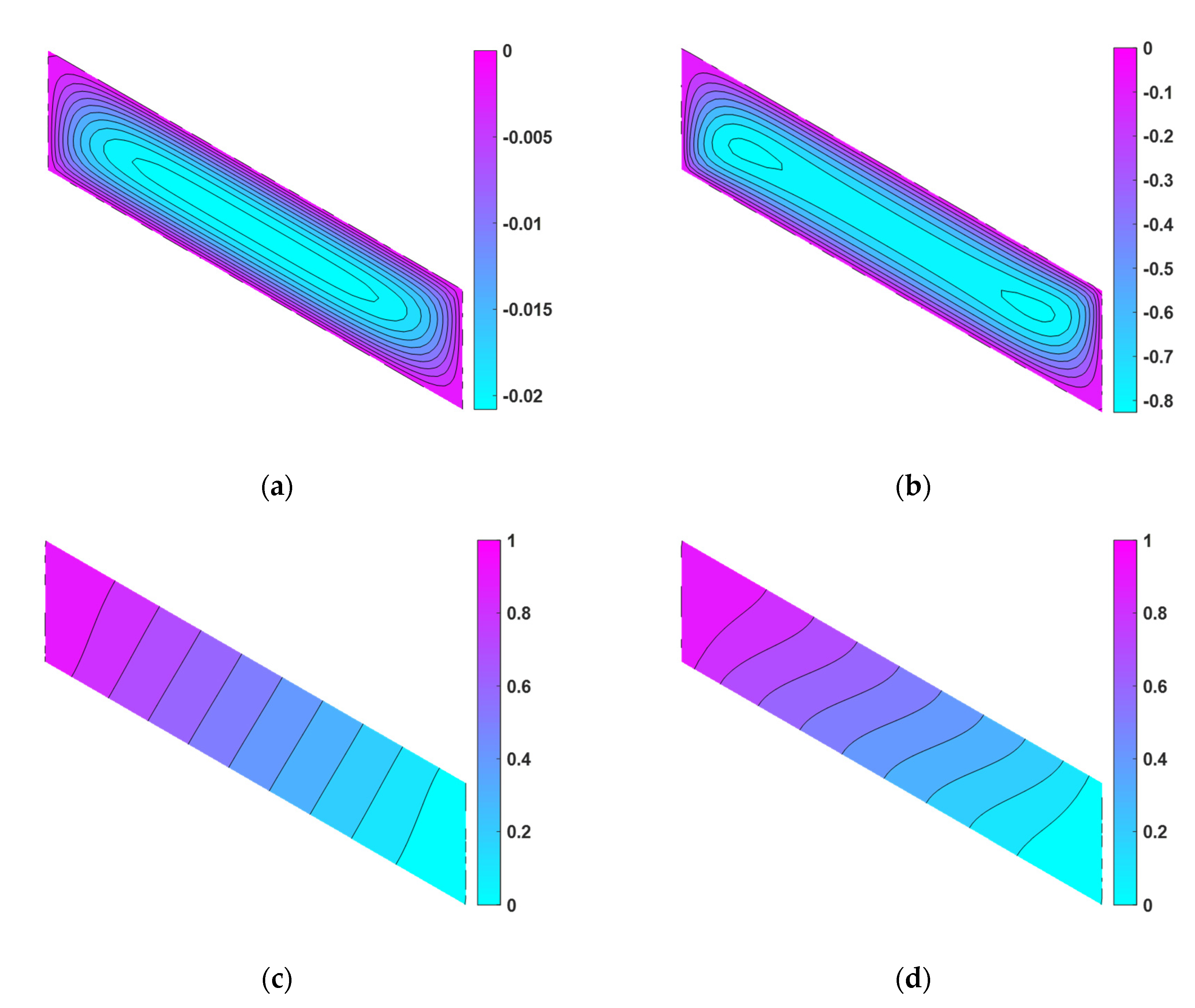
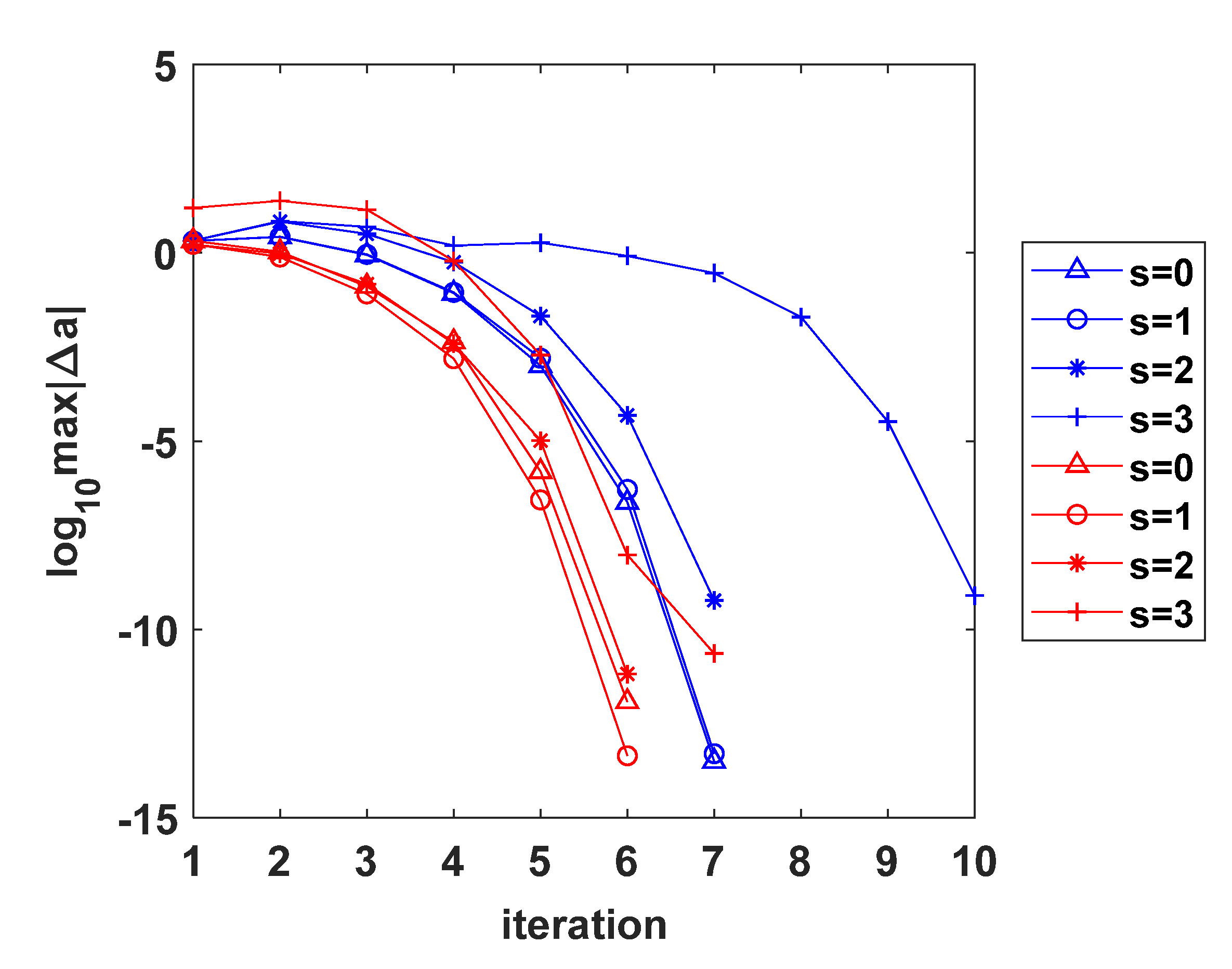
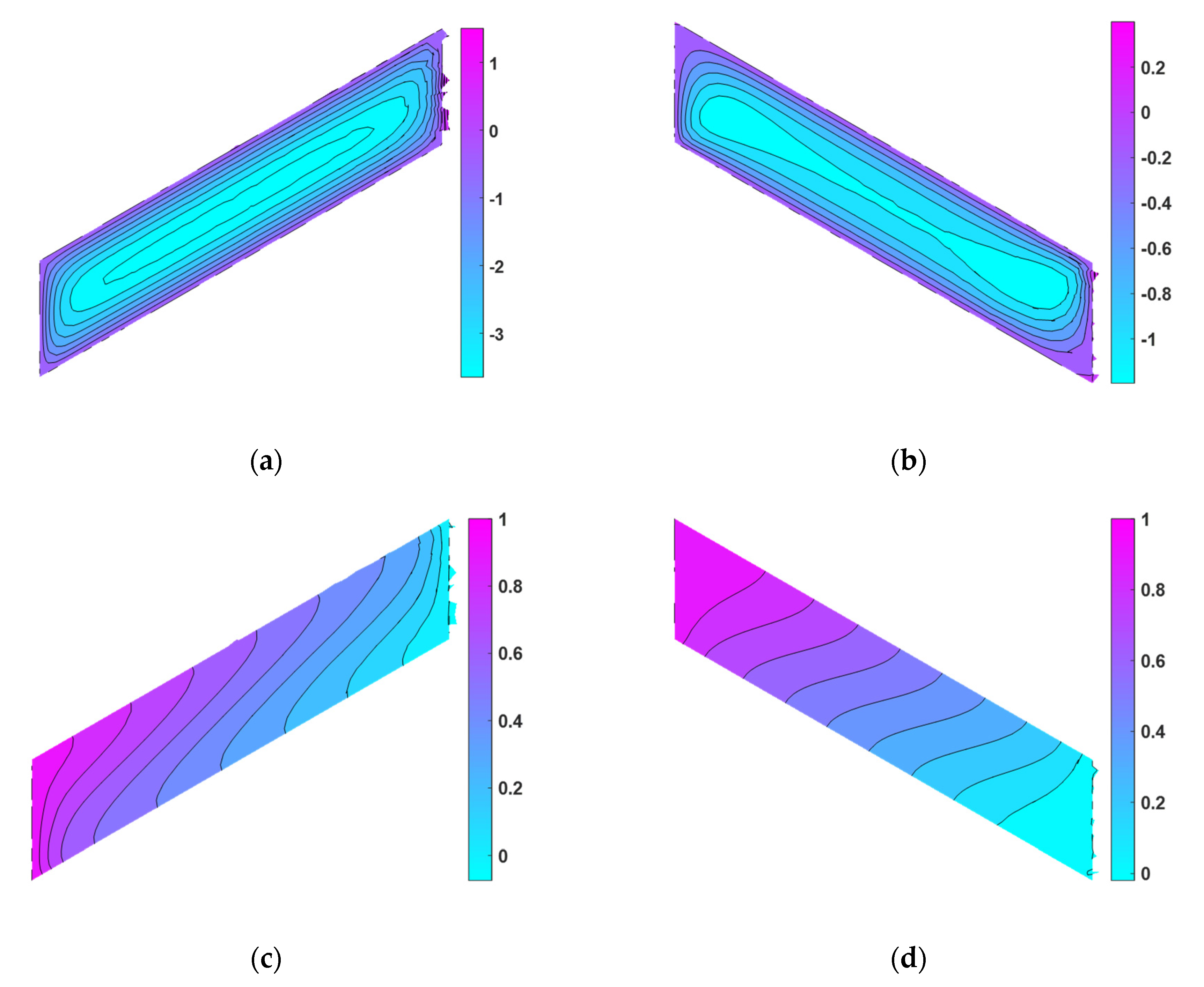
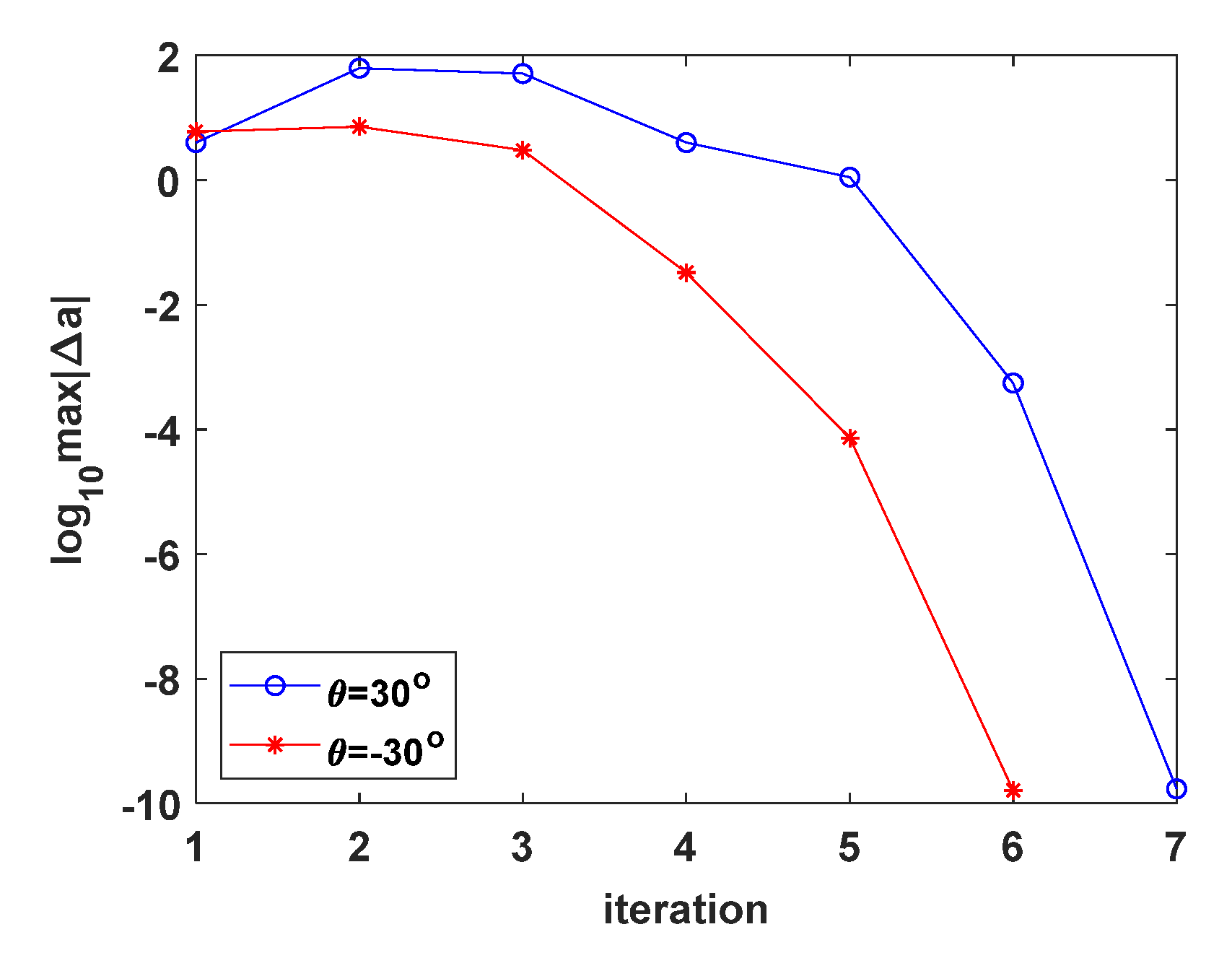
The disturbance of discretization is added to test the stability of the method. By using and with various , the convergence paths of two domains are compared in Figure 29; again, domain I shows slower convergence than domain II, and a larger requires more iterations. For illustration purpose, the non-uniform discretization obtained by is presented in Figure 30, and the corresponding contour plots of and are given in Figure 31. Similar trends in the distribution of both contours and are observed while the smoothness of the contours is reduced to some extent in comparison with those obtained by uniform discretization. Lastly, a higher level of disturbance is further investigated, as shown in Figure 32, which has not been discussed in the literature. It is found that the RK support size is not able to yield satisfactory results. Nevertheless, the flexibility of RKCM enables a larger support size in the approximation. When using , the contour plots of and are shown in Figure 33 with corresponding iteration given in Figure 34. The patterns of the contours are ensured.
5. Conclusions
The Newton–Raphson collocation method with reproducing kernel approximation is proposed to solve the natural convection problem within a parallelogrammic enclosure. Particularly, a nonlinear system is established on the basis of local approximation. In addition to the benchmark problems given in the literature, a unit square enclosure is designed to unveil the parameters in RKCM when nonlinearity is of importance in such a porous enclosure. From the parametric study, the convergence of the method is stable and efficient, regardless of various initial conditions, disturbance of discretization, inclination, aspect ratio, and the RK support size. Additionally, it is observed that the parameter controls the nonlinearity of the system. In all examples, as the value of increases, the magnitude of increases, and so does the nonlinearity of contour . Even so, the present method yields the desired accuracy for a large value of . Although the RK support size is not sensitive to uniformly discretized domains, for highly irregular discretization, it is shown that a larger support size in RKCM offers flexibility in yielding accurate approximation. The feasibility of the method for analyzing two-phase coupling problems is, therefore, demonstrated. To keep the article an adequate length, the extension to three-phase coupling problems, i.e., double-diffusive natural convection problems, is left to be investigated by future works.
Author Contributions
Funding acquisition, J.P.Y.; Investigation, Y.-S.L.; Methodology, J.P.Y.; Project administration, J.P.Y.; Supervision, J.P.Y.; Writing—original draft, J.P.Y.; Writing—review & editing, J.P.Y. All authors have read and agreed to the published version of the manuscript.
Funding
This research was funded by the Ministry of Science and Technology of the Republic of China (Taiwan) under grant number MOST 107-2221-E-009-141-MY3.
Conflicts of Interest
The authors declare no conflict of interest.
Appendix A
Explicit Expression for Matrix :
Explicit Expression for Matrix :
References
- Nithiarasu, P.; Seetharamu, K.N.; Sundararajan, T. Double-diffusive natural convection in an enclosure filled with fluid-saturated porous medium: A generalized non-Darcy approach. Numer. Heat Transf. A 1996, 30, 413–426. [Google Scholar] [CrossRef]
- Costa, V.A.F. Double-diffusive natural convection in parallelogrammic enclosures filled with fluid-saturated porous media. Int. J. Heat Mass Transf. 2004, 47, 2699–2714. [Google Scholar] [CrossRef]
- Chamkha, A.J. Double-diffusive convection in a porous enclosure with cooperating temperature and concentration gradients and heat generation or absorption effects. Numer. Heat Transf. A 2002, 41, 65–87. [Google Scholar] [CrossRef] [Green Version]
- Kramer, J.; Jecl, R.; Škerget, L. Boundary domain integral method for the study of double diffusive natural convection in porous media. Eng. Anal. Bound. Elem. 2007, 31, 897–905. [Google Scholar] [CrossRef]
- Stajnko, J.K.; Ravnik, J.; Jecl, R. Numerical simulation of three-dimensional double-diffusive natural convection in porous media by boundary element method. Eng. Anal. Bound. Elem. 2017, 76, 69–79. [Google Scholar] [CrossRef]
- Fan, C.M.; Chien, C.S.; Chan, H.F.; Chiu, C.L. The local RBF collocation method for solving the double-diffusive natural convection in fluid-saturated porous media. Int. J. Heat Mass Transf. 2013, 57, 500–503. [Google Scholar] [CrossRef]
- Li, P.W.; Chen, W.; Fu, Z.J.; Fan, C.M. Generalized finite difference method for solving the double-diffusive naturalconvection in fluid-saturated porous media. Eng. Anal. Bound. Elem. 2018, 95, 175–186. [Google Scholar] [CrossRef]
- Yang, J.P.; Su, W.T. Investigation of radial basis collocation method for incremental-iterative analysis. Int. J. Appl. Mech. 2016, 8, 1650007. [Google Scholar] [CrossRef]
- Yang, J.P.; Su, W.T. Strong-form framework for solving boundary value problems with geometric nonlinearity. Appl. Math. Mech. Engl. 2016, 37, 1707–1720. [Google Scholar] [CrossRef]
- Yang, J.P.; Chen, Y.C. Gradient enhanced localized radial basis collocation method for inverse analysis of Cauchy problems. Int. J. Appl. Mech. 2020, 12, 2050107. [Google Scholar] [CrossRef]
- Yang, J.P.; Guan, P.C.; Fan, C.M. Weighted reproducing kernel collocation method and error analysis for inverse Cauchy problems. Int. J. Appl. Mech. 2016, 8, 1650030. [Google Scholar] [CrossRef]
- Yang, J.P.; Hsin, W.C. Weighted reproducing kernel collocation method based on error analysis for solving inverse elasticity problems. Acta Mech. 2019, 230, 3477–3497. [Google Scholar] [CrossRef]
- Yang, J.P.; Lam, H.F.S. Detecting inverse boundaries by weighted high-order gradient collocation method. Mathematics 2020, 8, 1297. [Google Scholar] [CrossRef]
- Bataineh, A.S.; Isik, O.R.; Oqielat, M.A.; Hashim, I. An enhanced adaptive Bernstein collocation method for solving systems of ODEs. Mathematics 2021, 9, 425. [Google Scholar] [CrossRef]
- Brunner, H. The solution of systems of stiff nonlinear differential equations by recursive collocation using exponential functions. In Numerische Behandlung von Differentialgleichungen; Birkhäuser: Basel, Switzerland, 1975; pp. 29–44. [Google Scholar]
- Bülbül, B.; Sezer, M. A new approach to numerical solution of nonlinear Klein-Gordon equation. Math. Probl. Eng. 2013, 2013, 869749. [Google Scholar] [CrossRef]
- Biot, M.A. Theory of stability and consolidation of a porous medium under initial stress. J. Math. Mech. 1963, 12, 521–541. [Google Scholar]
- Haoyan, W.; Chen, J.S.; Hillman, M. A stabilized nodally integrated meshfree formulation for fully coupled hydro-mechanical analysis of fluid-saturated porous media. Comput. Fluids 2016, 141, 105–115. [Google Scholar]
- Chi, S.W.; Chen, J.S.; Hu, H.Y.; Yang, J.P. A gradient reproducing kernel collocation method for boundary value problems. Int. J. Numer. Meth. Eng. 2013, 93, 1381–1402. [Google Scholar] [CrossRef]
Figure 1.
Mathematical model: (a) geometry; (b) boundary conditions.

Figure 2.
Schematic diagram of collocation points.

Figure 3.
Schematic diagrams of the discretization in square domain: (a) uniform discretization; (b) non-uniform discretization.
Figure 3.
Schematic diagrams of the discretization in square domain: (a) uniform discretization; (b) non-uniform discretization.

Figure 4.
Various collocation points and corresponding iterations.

Figure 5.
Contour plots obtained by various collocation points: (a) by ; (b) by ; (c) by ; (d) by ; (e) by ; (f) by .
Figure 5.
Contour plots obtained by various collocation points: (a) by ; (b) by ; (c) by ; (d) by ; (e) by ; (f) by .

Figure 6.
Non-uniform discretization with various values and corresponding iterations.

Figure 7.
Contour plots obtained by non-uniform discretization: (a) ; (b) .

Figure 8.
Various RK support sizes and corresponding iterations.

Figure 9.
Various initial conditions and corresponding iterations.

Figure 10.
Various initial conditions in the discretized square domain: (a) schematic diagram; (b) iterations.
Figure 10.
Various initial conditions in the discretized square domain: (a) schematic diagram; (b) iterations.

Figure 11.
Various values and corresponding iterations.

Figure 12.
Contour plots obtained by various : (a) with ; (b) with ; (c) with ; (d) with .

Figure 13.
Schematic diagrams of the discretization in the diamond domain: (a) uniform discretization; (b) non-uniform discretization.
Figure 13.
Schematic diagrams of the discretization in the diamond domain: (a) uniform discretization; (b) non-uniform discretization.

Figure 14.
Various collocation points and corresponding iterations.

Figure 15.
Contour plots obtained by various collocation points: (a) by ; (b) by ; (c) by ; (d) by ; (e) by ; (f) by .
Figure 15.
Contour plots obtained by various collocation points: (a) by ; (b) by ; (c) by ; (d) by ; (e) by ; (f) by .

Figure 16.
Non-uniform discretization with various and corresponding iterations.

Figure 17.
Contour plots obtained by non-uniform discretization: (a) ; (b) .

Figure 18.
Various initial conditions and corresponding iterations.

Figure 19.
Various initial conditions in the discretized square domain: (a) schematic diagram; (b) iterations.
Figure 19.
Various initial conditions in the discretized square domain: (a) schematic diagram; (b) iterations.

Figure 20.
Various and corresponding iterations.

Figure 21.
Contour plots obtained by various : (a) with ; (b) with ; (c) with ; (d) with .


Figure 22.
Schematic diagrams of uniform discretization in the parallelograms: (a) domain I; (b) domain II.
Figure 22.
Schematic diagrams of uniform discretization in the parallelograms: (a) domain I; (b) domain II.

Figure 23.
Various collocation points and corresponding iterations.

Figure 24.
Contour plots obtained by uniform discretization with : (a) in domain I; (b) in domain II; (c) in domain I; (d) in domain II.
Figure 24.
Contour plots obtained by uniform discretization with : (a) in domain I; (b) in domain II; (c) in domain I; (d) in domain II.

Figure 25.
Various initial conditions and corresponding iterations: (a) ; (b) .

Figure 26.
Various and corresponding iterations.

Figure 27.
Contour plots obtained by various in domain I: (a) with ; (b) with ; (c) with ; (d) with .
Figure 27.
Contour plots obtained by various in domain I: (a) with ; (b) with ; (c) with ; (d) with .

Figure 28.
Contour plots obtained by various in domain II: (a) with ; (b) with ; (c) with ; (d) with .
Figure 28.
Contour plots obtained by various in domain II: (a) with ; (b) with ; (c) with ; (d) with .

Figure 29.
Non-uniform discretization with various values and corresponding iterations.

Figure 30.
Non-uniform discretization with in the parallelograms: (a) domain I; (b) domain II.

Figure 31.
Contour plots obtained by non-uniform discretization with : (a) in domain I; (b) in domain II; (c) in domain I; (d) in domain II.
Figure 31.
Contour plots obtained by non-uniform discretization with : (a) in domain I; (b) in domain II; (c) in domain I; (d) in domain II.

Figure 32.
Non-uniform discretization with in the parallelograms: (a) domain I; (b) domain II.

Figure 33.
Contour plots obtained by non-uniform discretization with : (a) in domain I; (b) in domain II; (c) in domain I; (d) in domain II.
Figure 33.
Contour plots obtained by non-uniform discretization with : (a) in domain I; (b) in domain II; (c) in domain I; (d) in domain II.

Figure 34.
Non-uniform discretization with and corresponding iterations.

Publisher’s Note: MDPI stays neutral with regard to jurisdictional claims in published maps and institutional affiliations. |
© 2021 by the authors. Licensee MDPI, Basel, Switzerland. This article is an open access article distributed under the terms and conditions of the Creative Commons Attribution (CC BY) license (https://creativecommons.org/licenses/by/4.0/).
Share and Cite
MDPI and ACS Style
Yang, J.P.; Liao, Y.-S. Direct Collocation with Reproducing Kernel Approximation for Two-Phase Coupling System in a Porous Enclosure. Mathematics 2021, 9, 897. https://0-doi-org.brum.beds.ac.uk/10.3390/math9080897
AMA Style
Yang JP, Liao Y-S. Direct Collocation with Reproducing Kernel Approximation for Two-Phase Coupling System in a Porous Enclosure. Mathematics. 2021; 9(8):897. https://0-doi-org.brum.beds.ac.uk/10.3390/math9080897
Chicago/Turabian StyleYang, Judy P., and Yi-Shan Liao. 2021. "Direct Collocation with Reproducing Kernel Approximation for Two-Phase Coupling System in a Porous Enclosure" Mathematics 9, no. 8: 897. https://0-doi-org.brum.beds.ac.uk/10.3390/math9080897
Note that from the first issue of 2016, this journal uses article numbers instead of page numbers. See further details here.