
A Plankton Detection Method Based on Neural Networks and Digital Holographic Imaging


1
Key Laboratory of Ocean Observation-Imaging Testbed of Zhejiang Province, Zhejiang University, Zhoushan 316021, China
2
The Engineering Research Center of Oceanic Sensing Technology and Equipment, Ministry of Education, Zhoushan 316021, China
3
Ocean College, Zhejiang University, Zhoushan 316021, China
*
Author to whom correspondence should be addressed.
Chemosensors 2022, 10(6), 217; https://0-doi-org.brum.beds.ac.uk/10.3390/chemosensors10060217
Submission received: 30 April 2022
/
Revised: 28 May 2022
/
Accepted: 6 June 2022
/
Published: 8 June 2022
(This article belongs to the Section Applied Chemical Sensors)
Abstract
:Detecting marine plankton by means of digital holographic microscopy (DHM) has been successfully deployed in recent decades; however, in most previous studies, the identification of the position, shape, and size of plankton has been neglected, which may negate some of the advantages of DHM. Therefore, the procedure of image fusion has been added between the reconstruction of initial holograms and the final identification, which could help present all the images of plankton clearly in a volume of seawater. A new image fusion method called digital holographic microscopy-fully convolutional networks (DHM-FCN) is proposed, which is based on the improved fully convolutional networks (FCN). The DHM-FCN model runs 20 times faster than traditional image fusion methods and suppresses the noise in the holograms. All plankton in a 2 mm thick water body could be clearly represented in the fusion image. The edges of the plankton in the DHM-FCN fusion image are continuous and clear without speckle noise inside. The neural network model, YOLOv4, for plankton identification and localization, was established. A mean average precision (mAP) of 97.69% was obtained for five species, Alexandrium tamarense, Chattonella marina, Mesodinium rubrum, Scrippsiella trochoidea, and Prorocentrum lima. The results of this study could provide a fast image fusion method and a visual method to detect organisms in water.
1. Introduction
Plankton are a crucial component of the global ecology and play essential roles in carbon, nutrient cycling, and food chains [1,2]. Marine plankton is vital for assessing the water and aquatic ecosystem quality because of their short lifespan and strong sensitivity to environmental conditions [3]. Mesodinium rubrum is a phototrophic ciliate that hosts cryptophyte symbionts and is well known for its ability to form dense harmful algae blooms (HABs) worldwide [4]. Chattonella blooms have been associated with serious economic damage to the Japanese aquaculture industry since 1972 [5]. Therefore, a robust method for detecting plankton is of great importance for monitoring the marine ecological environment.
Several technologies for plankton monitoring have been established, such as traditional microscope technologies [6,7,8], the FlowCAM tool [9,10,11], fluorescence analysis, etc [12,13]. Traditional microscope technologies on the basis of computer vision have been popular in recent years; however, when photographing plankton, the field of view is limited and only the cell in the focal plane is imaged clearly [8]. FlowCAM can analyze particles or cells in a moving fluid. However, the accuracy of detection is greatly affected by undesirable particles, such as air bubbles entering the pump, which are also detected as plankton [11]. Moreover, the structure of the plankton may be destroyed when entering the pump. Fluorescence-based approaches to monitoring plankton rely on chlorophyll a, phycocyanin, or other photosynthetic pigments, however, they are restrained by the range of concentrations they can detect [12].
Digital holography (DH) is a powerful technology for recording three-dimensional (3D) information through light interference and diffraction. The volume of water that can be imaged with DHM is much larger than with conventional optical microscopy. In recent years, with the development of digital holographic imaging technology, a large number of studies have been carried out using underwater digital holographic imaging. D.W. Pfitsch et al. used a submersible, free-drifting, digital holographic cinematography system that has a real-time fiber optic communication link, and captured images of medusa [14]. Andrea et al. proposed a method based on DHM for microalgae biovolume assessment [15]. Siddharth et al. deployed a holography system called Holosub in Eastsound, Washington, and captured more than 20,000 holograms, including Noctiluca cells, nauplii, calanoid copepod, etc. [16]. Previous studies have shown that DHM has great potential for plankton monitoring [14,15,16].
Compared with traditional optical microscopy, DHM has great advantages for analyzing the shape, size, density, and position of plankton due to its 3D information recording [14]. During hologram processing, holograms are first reconstructed [14,15,16]. The original holograms record all information about water bodies of a certain thickness, which means that information about a great number of object planes in the water is recorded on the hologram plane. To recover information on each object plane, the holograms are reconstructed according to the numerical propagation distance between the object and the hologram planes. A series of reconstructed images are obtained. However, only a portion of the cells is clear in each reconstructed image because the cells are in different focal planes of the water body. Hence, many studies have only extracted the regions of clear cells as regions of interest (ROIs) in each reconstructed image; finally collecting all the sub-images of ROIs together to represent all plankton information in the target water body [14,16]. However, this may increase computing time due to the involvement of sub-image cropping. Additionally, these methods only provide information on the density and categories of plankton but sacrifice information on the 3D position and size, which weakens the advantages of DHM.
Therefore, image fusion technology is integrated to fuse all the reconstructed images into an image and make sure all observed plankton cells are clearly represented in the same fusion image. The use of traditional image fusion methods, such as the wavelet transform (WT) image fusion method, to process reconstructed images, introduces speckle noise inside the plankton and diffraction fringes around the plankton cells and causes the edges of the plankton to become discontinuous [17,18,19]. A new image fusion method, ‘DHM-FCN’, based on improved FCN is proposed, which not only runs faster than the WT method but also suppresses background and speckle noises [20]. In DHM-FCN, the application of a weight matrix enables fusion images to obtain clear cells from the corresponding reconstructed images. The weighted calculations smooth out high-frequency noise in holographic backgrounds and diffraction fringes around the plankton cells.
Here, a monitoring approach for microplankton is proposed that could be used to analyze much larger water bodies, which contain the 3D information by means of DHM. The resolution of the imaging system is greater than 1 µm. Instead of cropping the holograms, the DHM-FCN method fuses all the reconstructed holograms of different object planes. The fusion images give information on the shapes, sizes, density, categories, and positions of the cells in the imaged water body. This method is simple and efficient. For plankton detection, a state-of-the-art object detection algorithm, YOLOv4, is used in this study, which can classify and locate the plankton in the images [21].
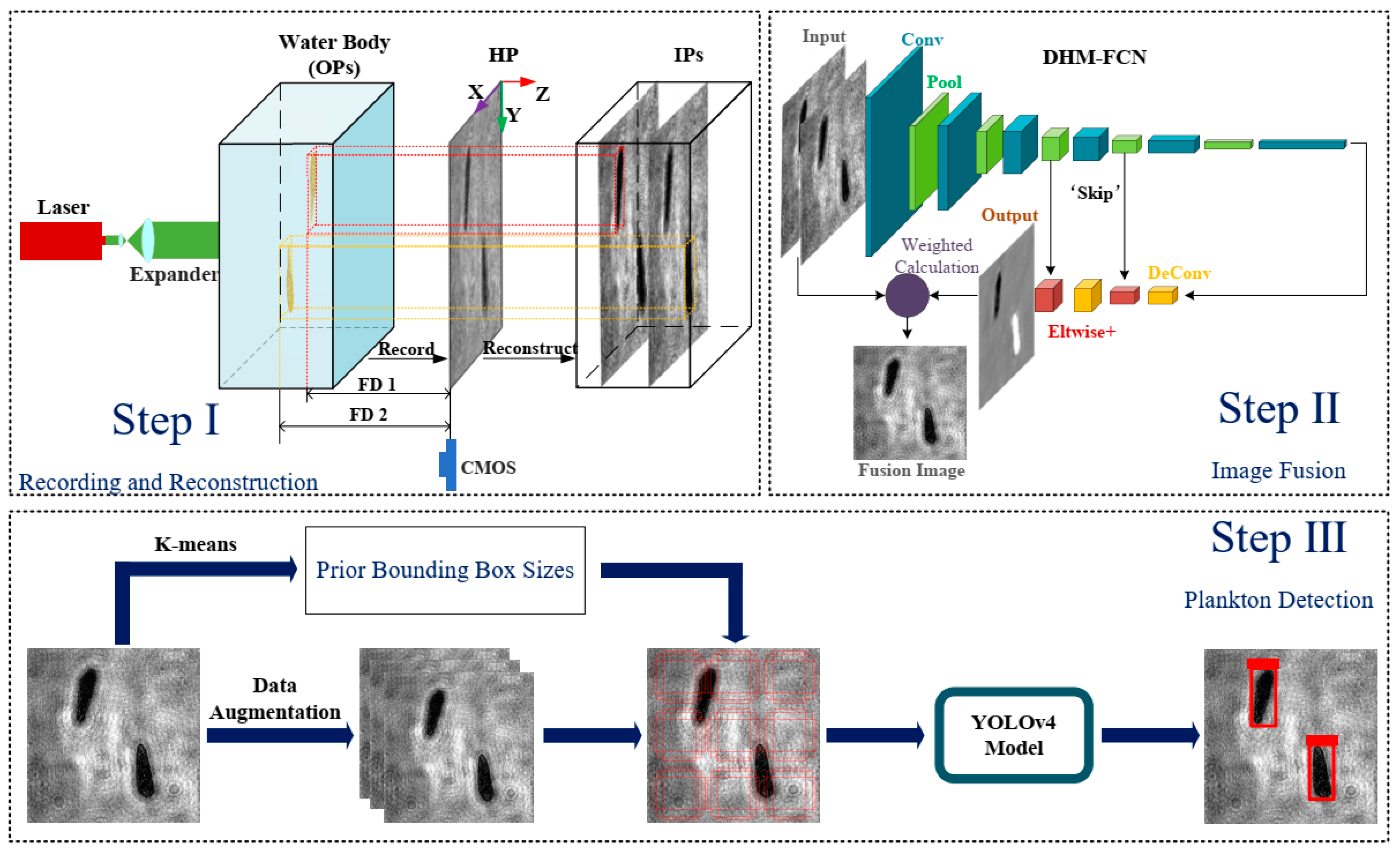
The structure of the paper is as follows. Section 2 describes the microplankton species and establishes the optical system and image processing. In Section 3, the proposed method for plankton detection is presented, including the image fusion method and the object detection method. The results of the proposed method and the comparison of different image fusion methods are presented in Section 4. Finally, the conclusions are given in Section 5. The procedures of plankton detection are shown in Figure 1.
2. Works Related to Data Acquisition
2.1. Microplankton Species
Five plankton species, Alexandrium tamarense (ATEC), Chattonella marina (CMSH), Mesodinium rubrum (JAMR), Scrippsiella trochoidea (STNJ), and Prorocentrum lima (PLGD), were selected as target species, which range in size from ~10 µm to 70 µm. JAMR were maintained in an f/2-Si medium at 17 °C, 30‰, and 54 µmol m−2s−1 of light intensity with a 14:10 light: dark cycle. The others were monoculture single cells isolated from the East China coast and were maintained in an f/2 medium at 20 °C, 30‰, and 100 µmol m−2s−1 of light intensity, with a 12:12 light: dark cycle. All species are common plankton in China. STNJ, ATEC, CMSH, and PLGD are harmful algae bloom species that are all toxic, except for STNJ.
2.2. The Optical System of DHM
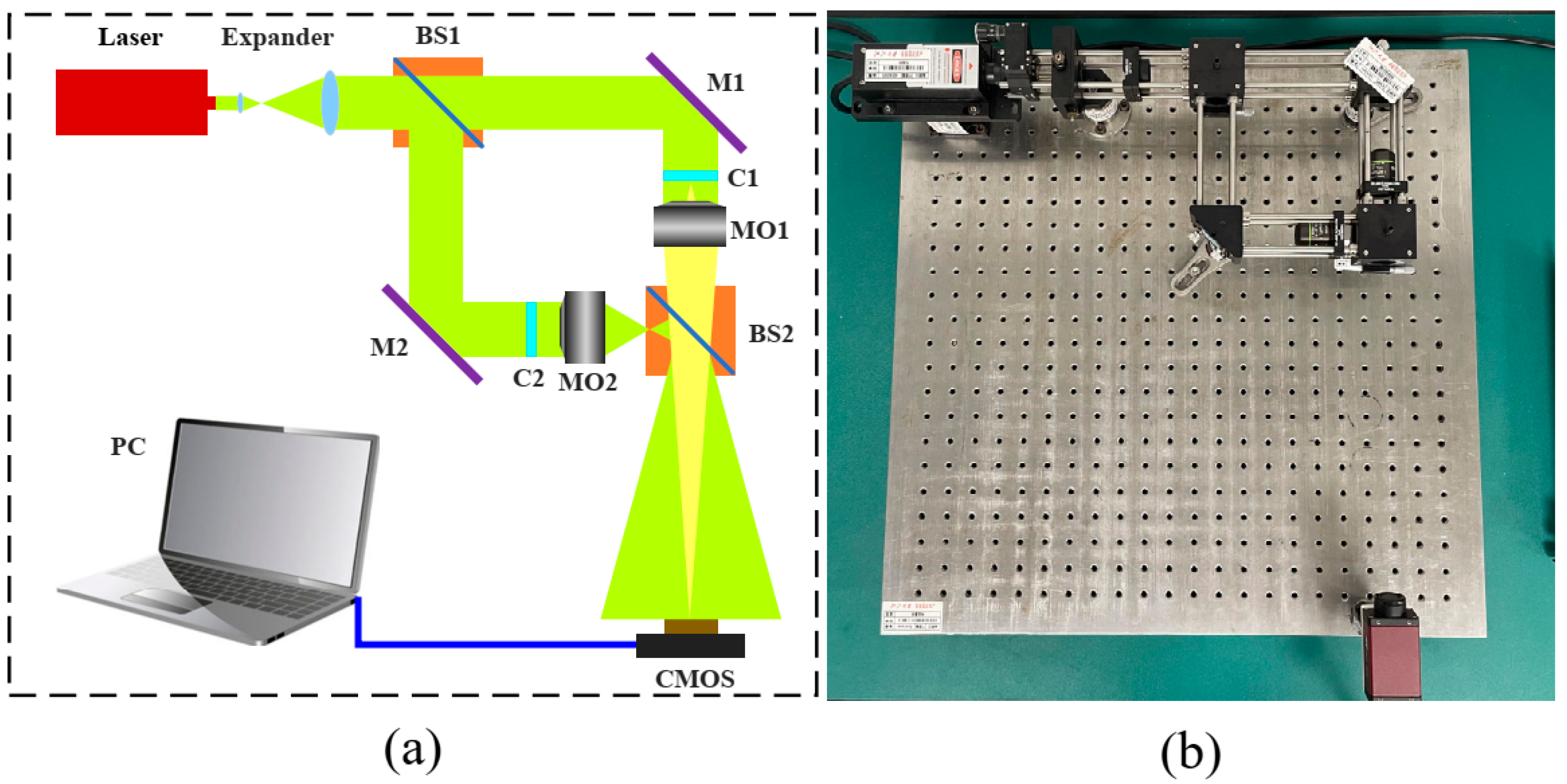
A coaxial optical path based on a Mach–Zendel interferometer structure was set up to obtain the best interference and highest interference contrast. The object and reference beams of the structure were strictly coaxial. Figure 2a shows a diagram of the DHM optical system and Figure 2b shows the setup of the experimental device. After passing through the expander, the laser (wavelength λ = 532 nm) is divided into an object beam and a reference beam using a beam splitter (BS). The cuvettes with the sample and reference liquids were set at the C1 and C2 positions, respectively. The beams passed through the cuvettes and microscope objectives (MO) and interfered after passing through the BS. To obtain a holographic image of the plankton, the interference pattern was recorded using a CMOS camera (AVT Manta G-419B PoE, 2048 × 2048, 5.5 µm × 5.5 µm pixels). The purpose of the cuvette with reference liquid is to minimize the impact of the liquid on imaging. The magnification of this optical system is 32.8 times. The optical path length of the cuvette is 2 mm.
2.3. Image Process
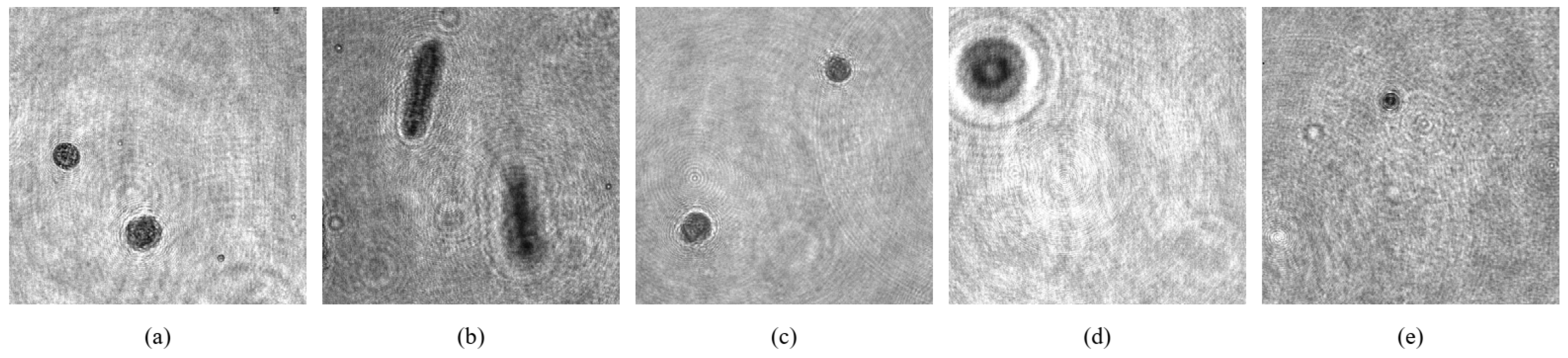
The procedures for plankton detection are divided into three key steps. Step I consists of the hologram acquisition and reconstruction, which is shown in Figure 1. The holograms are captured by a CMOS camera that records the amplitude and phase information of the object’s light field. A total of 1771 original holograms were acquired using the setup introduced in Section 2.2, including 335 for ATEC, 451 for CMSH, 415 for JAMR, 251 for PLGD, and 319 for STNJ. The image planes of the different focus distances were recovered from the original holograms using reconstruction algorithms. The holograms of the five plankton species are shown in Figure 3.
Reconstruction
A hologram recorded the complex wave-front of the water body on the CMOS camera and the intensity and phase of the cells in it could be recovered via the numerical reconstruction of the hologram. Each reconstructed hologram recovered one object plane according to the focus distance, which was the actual optical path length from the object plane to the CMOS plane. Various methods can be used to perform the reconstruction, such as the convolution method (CM), the Fresnel transformation method (FTM), and the angular spectrum method (ASM) [22,23]. The size of the reconstructed holograms obtained by CM is consistent with the original holograms. However, CM takes a long time to reconstruct and would cause spectrum under-sampling. FTM is a rapid method for reconstruction; however, the size of the reconstructed holograms varies with the reconstructed distance, which results in poor reconstructed hologram quality. ASM was applied in this study due to its strong ability to suppress the under-sampling problem, fast speed, and the consistent size of the images. ASM was employed to reconstruct the complex amplitude of the object, which is expressed as:
where and denote the Fourier transform and the inverse Fourier transform, respectively, is the frequency filter used to obtain the +1 order spectrum or the −1 order spectrum of the object, λ is the wavelength of the light source, z is the numerical propagation distance, and is the optical transfer function in the frequency domain corresponding to the propagation distance. The codes of ASM were established by our team according to Equation (1). As can be seen in Figure 1, reconstructed holograms with different focus distances were obtained from one hologram. It takes 0.2858 s to obtain a reconstructed image on a computer with a GeForce GTX 1660 graphics card, 8.00 GB of RAM, i5-9400F 2.90 GHz processor, and 64 nuclear CPU.
3. Proposed Method for Plankton Detection
In step II, a new imaged fusion method, ‘DHM-FCN’, is proposed to fuse two reconstructed holograms of different object planes at one time. The fusion image contains all the in-focus cells in the imaged water. In the last step, the images in the dataset are analyzed by K-means clustering, to obtain the sizes of the prior bounding boxes [24]. The detection model is trained with the bounding boxes and the dataset. The images are detected by the YOLOv4 and in this way, the graphical results about the categories, density, positions, shapes, and sizes of plankton in the imaged water are obtained. The two steps are shown in Figure 1.
3.1. Image Fusion
Image fusion combines information from multi-focus images of the same scene. The result of image fusion is a single image, which contains a more accurate description of the scene than any of the individual source images. This fused image is more useful and suitable for human vision, machine perception, or further image processing tasks [25]. For hologram processing, image fusion combines the reconstructed holograms of different object planes and brings all observed plankton cells into focus to be represented in a fusion image. Image fusion for reconstructed holograms was carried out by various algorithms, such as wavelet transform, which fuse the source images in the wavelet domain according to fusion rules [26]. In this paper, a new image fusion method, ‘DHM-FCN’, was proposed, and the DHM-FCN method was compared to the methods based on wavelet transformation with different rules and the pulse-coupled neural networks (PCNN) method [27].
The improved neural network is based on FCN that takes inputs of arbitrary size and produces corresponding-sized outputs with efficient inference and learning. In this study, the inputs of the network are two reconstructed holograms with different focus distances from one original hologram. The output of the neural network is the fusion weight matrix of the inputs. The weights of the focused plankton regions in the first reconstructed hologram were set to 0 and the weights of the in-focus plankton regions in the second reconstructed hologram were set to 1. The other regions were the background and their weight values were set to 0.5. The diffraction fringes in the background of different reconstructed images are different. In order to smooth the high-frequency diffraction fringes in the background, the weight values of the background are important. Taking the weight matrix as the pixel value matrix of the grayscale image, a visual representation of the weight matrix can be obtained, which is called a label graph, as shown in Figure 5.
In order to speed up the algorithm, a simple structure was adopted for the neural network. The trainable parameters of the traditional FCN model for weight matrix regression are compared with the DHM-FCN model in Table 1. The simplified structure of DHM-FCN greatly increased the speed of the algorithm and reduced the time required for training. Considering the limitations of the device and the speed of the algorithm, the input of this experiment was uniformly scaled to 512 × 512.
The structure diagram of the neural network is shown in Figure 1. Each layer of data is a three-dimensional array of size h × w × d, where h and w are spatial dimensions and d is the feature or channel dimension. The first layer is the input, with a pixel size of 512 × 512 and two channels. The convolution layers are used to extract the image features. The functions of the pooling layers are to select the features extracted from the convolution layer, reduce the feature dimension, and avoid overfitting. Deconvolution layers are used to restore the size of the feature map and achieve the regression of weight values. The skip architecture defined in DHM-FCN uses eltwise+ layers that combine different feature maps to better regress the weight matrix. In the network, up-sampling layers enable weight value regression and learning in nets with subsampled pooling. The last layer is output, which is the weight matrix of the input images used for the reconstructed holograms’ fusion.
The fused image is expressed as:
where denotes that all the elements in the matrix are 1. and are the first and second reconstructed holograms, respectively. is the weight matrix of and obtained from the DHM-FCN. The structure of the DHM-FCN is shown in Table 2.
Training of the DHM-FCN model: In this work, each set of data contained two reconstructed holograms and the corresponding manual weight matrix during training. The two reconstructed holograms in each group corresponded to different reconstruction distances of the same hologram. An optimizer that implements the Adam algorithm was used. The batch size was set to 1 with an initial learning rate of 0.001. The loss function was a mean square error:
where m and n denote the scales of the weight matrix. and are the predicted weight value and the real weight value. The DHM-FCN model with the loss function achieved the regression of the weight values in the weight matrix.
3.2. Object Detection
In the past several years, computer versions, especially object detection, boomed with the development of computers. There are two types of object detection algorithms based on deep learning: two-stage object detection algorithms and one-stage object detection algorithms [28,29]. The two-stage algorithms generate a candidate region that contains the object to be detected after the feature extraction in the first step, and the second step performs the classification and localization regression through the classifiers. Two-stage algorithms include regional convolutional neural networks (R-CNN) [30], SPP-Net [31], fast regional convolutional neural networks (Fast R-CNN) [32], faster regional convolutional neural networks (Faster R-CNN) [29], etc. Such algorithms are characterized by high accuracy but slow speed. The one-stage algorithms do not generate candidate regions but directly classify and locate them after feature extraction. These algorithms run faster than the two-stage algorithms. Many researchers have improved the one-stage algorithms, and now the one-stage algorithm performs well on object detection tasks in various fields. Examples of one-stage neural networks include SSD [28], YOLO [33] and YOLOv4 [21].
The original YOLO model that was used for object detection was developed by Joseph et al. in 2016 [33]. Many have subsequently improved on this model [34,35]. The model used in this paper was YOLOv4, which was an object detector in production systems with optimization for parallel computations and fast operating speed, developed by Alexey et al. in 2020 [21]. YOLOv4 can be trained and used with a conventional GPU with 8–16 GB-VRAM.
YOLOv4 is divided into three parts: the backbone, neck, and head. The backbone of the network is responsible for extracting features from the image, which largely determines the performance of the detector. Generally, the backbone is a convolutional neural network (CNN) that has been pre-trained on ImageNet [36] or COCO [37] datasets. The head is the network layers that are randomly initialized during training after the backbone to make up for the defects that CNN cannot locate. Between the backbone and the head, some network layers are added to collect feature maps in different stages, usually called the neck.
YOLOv4 uses CSPDarknet53 [38] as the backbone, which is pre-trained on ImageNet, SPP [31] additional module and PANet [39] path-aggregation as the neck, and YOLOv3 (anchor-based) head, which is used to predict the classes and bounding boxes of objects.
Acquisition of prior bounding box: A prior bounding box is a bounding box with different sizes and different aspect ratios, which is preset in the image in advance. The detectors predict whether the box contains plankton and its coordinates. Prior bounding boxes allow the model to learn more easily. Setting prior bounding boxes of different scales increases the probability of a box that has a good match for the target object appearing. It is crucial to select the number and size of bounding boxes. In this paper, K-means clustering is used instead of manually designing anchors [24]. By clustering the bounding box of the training dataset, a set of bounding boxes that are more suitable for the dataset are automatically generated, which makes the detection effect of the network better. The K-means algorithm divides the data into k categories, where k needs to be preset. The length and width of plankton in the training dataset were used as initial data to experiment with K-means.
Training of the YOLOv4 model: To improve the speed of the detection algorithm, the input of YOLOv4 was scaled to 608 × 608. The transfer learning method was applied to speed up and optimize the learning efficiency instead of training the model with randomly initialized weights from scratch, which was a technology that took the well-trained model parameters as the initial values of our own model parameters. The loss was divided into three parts: location, confidence, and category loss. In this study, the loss function adopted was proposed by Alexey et al. [21].
Evaluation criteria: Recall, average precision (AP), and the F1 score were used to evaluate the performance of the neural networks in this paper. Recall was expressed as:
where TP is the number of positive samples that were correctly predicted and FN is the number of samples belonging to positive samples that were predicted to be negative.
IOU refers to the ratio of the overlapping area to the combined area of the two bounding boxes. AP is an evaluation index that comprehensively considers recall and accuracy. They are expressed as:
where TB means truth boxes and PB means predicted boxes. Additionally, t indicates that when the IOU is larger than t, the prediction is assumed to have correctly detected this target. Furthermore, p(t) is the precision when the recall is r(t). The F1 score is an evaluation index combining precision and recall. The F1 score is defined as follows:
The location of the cell was evaluated by the focus distance and the coordinates of object detection bounding boxes. The size of the cells was evaluated by the size of the bounding box and the optical system parameters, which were expressed as:
where IR is the scale of the original hologram, PS is the size of the pixel, Mag is the magnification of the optical system, and Sc is the scale of the detector’s input.
4. Results and Discussion
4.1. Image Fusion Method
Data augmentation: The data for image fusion were reconstructed holograms. Neural networks’ performance highly depends on the training dataset’s size. Large datasets can increase the performance of the networks. To obtain as many images as possible, the data augmentation method was applied to enlarge the dataset. In this study, there are a total of 2464 reconstructed holograms in groups of 1232. Brightness adjustment, horizontal flip, vertical flip, and diagonal flip technologies were used for image augmentation. The dataset was divided into 80% for training the model, 10% for validation, and 10% for testing.
Comparison of Different Image Fusion Methods
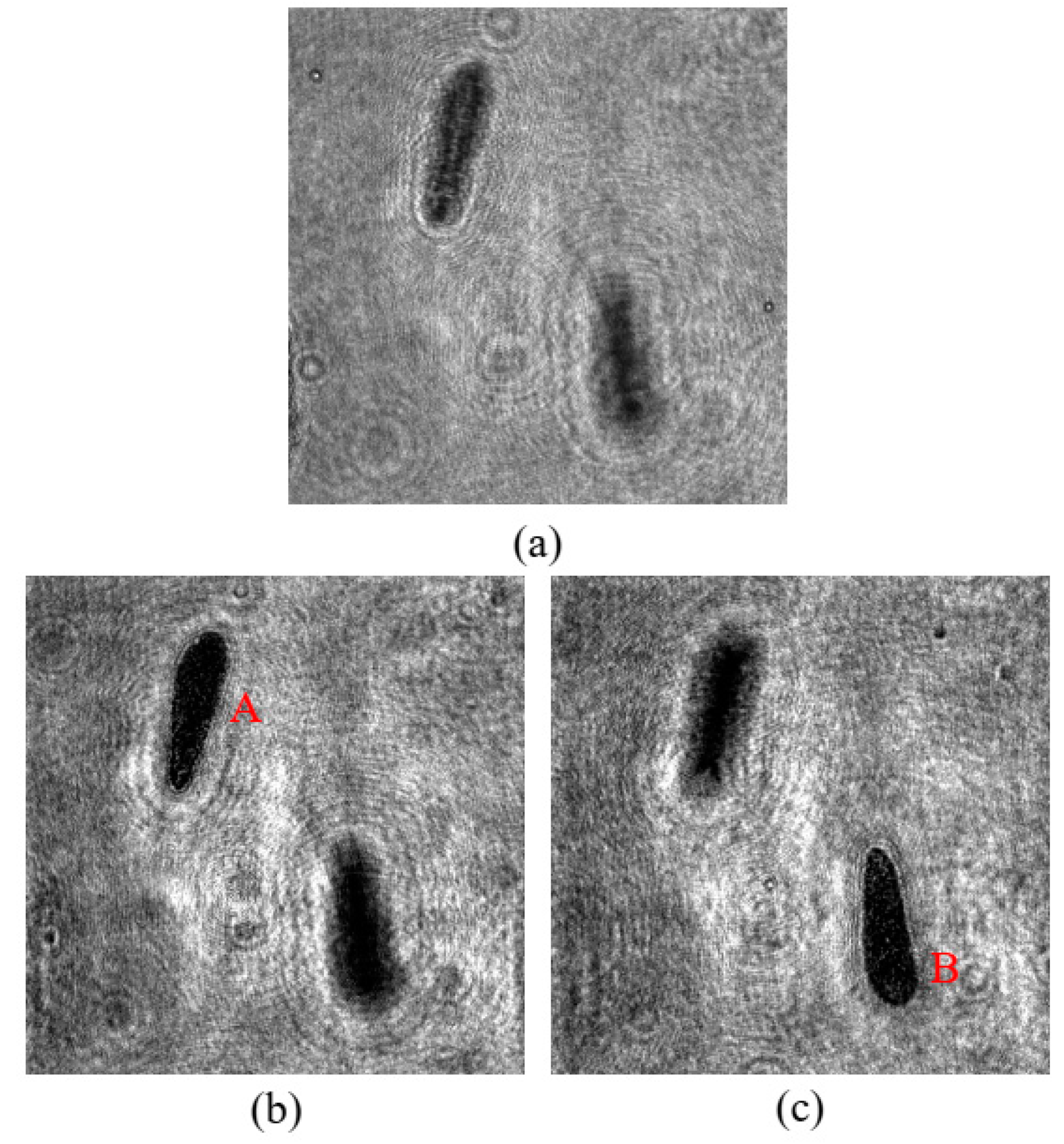
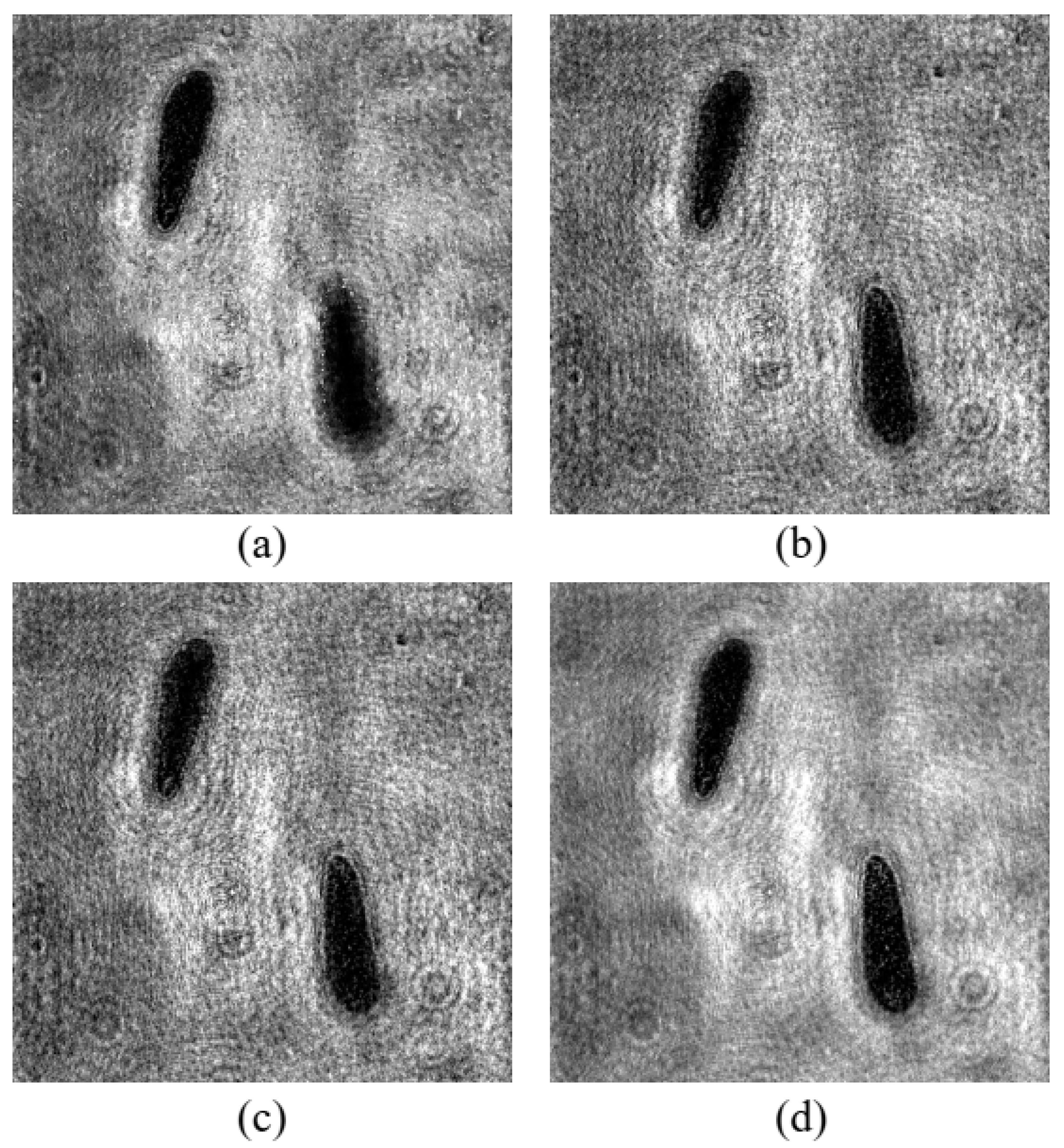
In this study, several image fusion methods were compared in terms of their processing speed and fusion effects. The inputs of all algorithms are shown in Figure 4b,c. The results of different methods are shown in Figure 6. Figure 6a,d are the results of PCNN, the regional wavelet transformation method (RW) [27], the pixel wavelet transformation method [19] and the method proposed in this paper (DHM-FCN), respectively. The weight matrix obtained by DHM-FCN is shown in Figure 5. PW considers the coefficients of each pixel individually. RW divides the sub-images of the original image into different regions and determines the overall coefficient of the entire region according to the regional characteristics.
The time required by the different algorithms to process image fusion on the same computer is listed in Table 3. The structural similarity (SSIM) and image correlation coefficient (Cor) between the result and the input images were used to evaluate the performance of the algorithms. The peak signal to noise ratio (PSNR) was also used.
All the image fusion methods mentioned above fuse two reconstructed holograms every time. The density of plankton is generally low in seawater, and it is rare for a hologram to contain more than two cells. However, during occurrences of harmful algae blooms, the density of plankton increases. In this case, two reconstructed holograms are fused and this fusion image is fused with the third reconstructed hologram until the fusion images obtained contain all the in-focus cells in the imaged water.
In the reconstructed holograms, the regions of blurred cells contained high-frequency diffraction fringes around plankton. Since the fusion of the high-frequency part by the WT method takes the maximum value, the pixels of the in-focus cells in the fused image are from the corresponding clearly reconstructed image and the pixels surrounding the cells are from the blurred reconstructed image. Speckle noise was caused by the fact that some pixels inside the clear plankton were taken from the blurred reconstructed image. This resulted in high-frequency diffraction fringes around the focused plankton and speckle noise in the fusion image, which degraded the quality of the result.
The weighted calculation of the reconstructed image with the weight matrix smoothed the background noise. DHM-FCN overcomes the problems of speckle noise and diffraction fringes in the wavelet transform method and discontinuous edge in PCNN. It is particularly important for microplankton detection, such as STNJ and ATEC, which are small and similar in morphology. If speckle noise is generated in the plankton, a lot of information can be lost, resulting in inaccurate identification.
DHM-FCN can quickly generate high-quality fusion images, which lays the foundation for the next step in object detection. Visually, DHM-FCN can effectively suppress background noise compared with other methods and the original images, and obtain more continuous cell boundaries. Statistically speaking, the large SSIM, Cor, and PSNR of DHM-FCN mean that this method recovers the plankton information from the input images efficaciously. DHM-FCN represents a significant improvement in the performance of fusion according to the evaluation metrics. DHM-FCN is 20 times faster than PW and RW and 5 times faster than PCNN. In this study, we adopted the DHM-FCN method to fuse the reconstructed images.
4.2. Object Detection
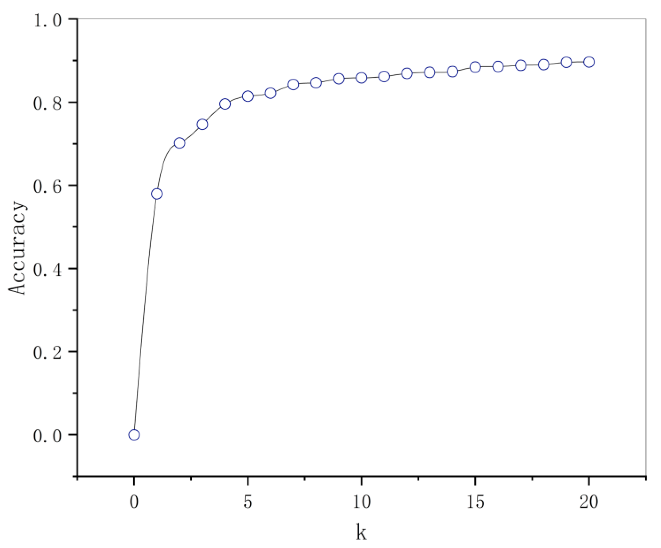
The experimental results of K-means are presented in Figure 7. By setting more bounding boxes, the performance of the model was improved to a certain extent, however, the complexity increased. To balance the accuracy and complexity of the model, k = 9 was finally selected, where the categories were 40 × 45, 42 × 39, 46 × 53, 51 × 43, 57 × 57, 65 × 65, 67 × 169, 83 × 87, and 116 × 142.
For data augmentation, the mosaic method of data augmentation used in this paper was a new technology proposed in YOLOv4. This method randomly uses four images for scaling, distribution, and stitching, which greatly enriched the detection dataset. In particular, random scaling added a lot of small targets, making the network more robust. The input data were the fusion images and the reconstructed holograms that only contained one cell. This differs from the dataset of DHM-FCN. The size of the original dataset was 1771. The dataset was divided into 80% for training the model, 10% for validation, and 10% for testing.
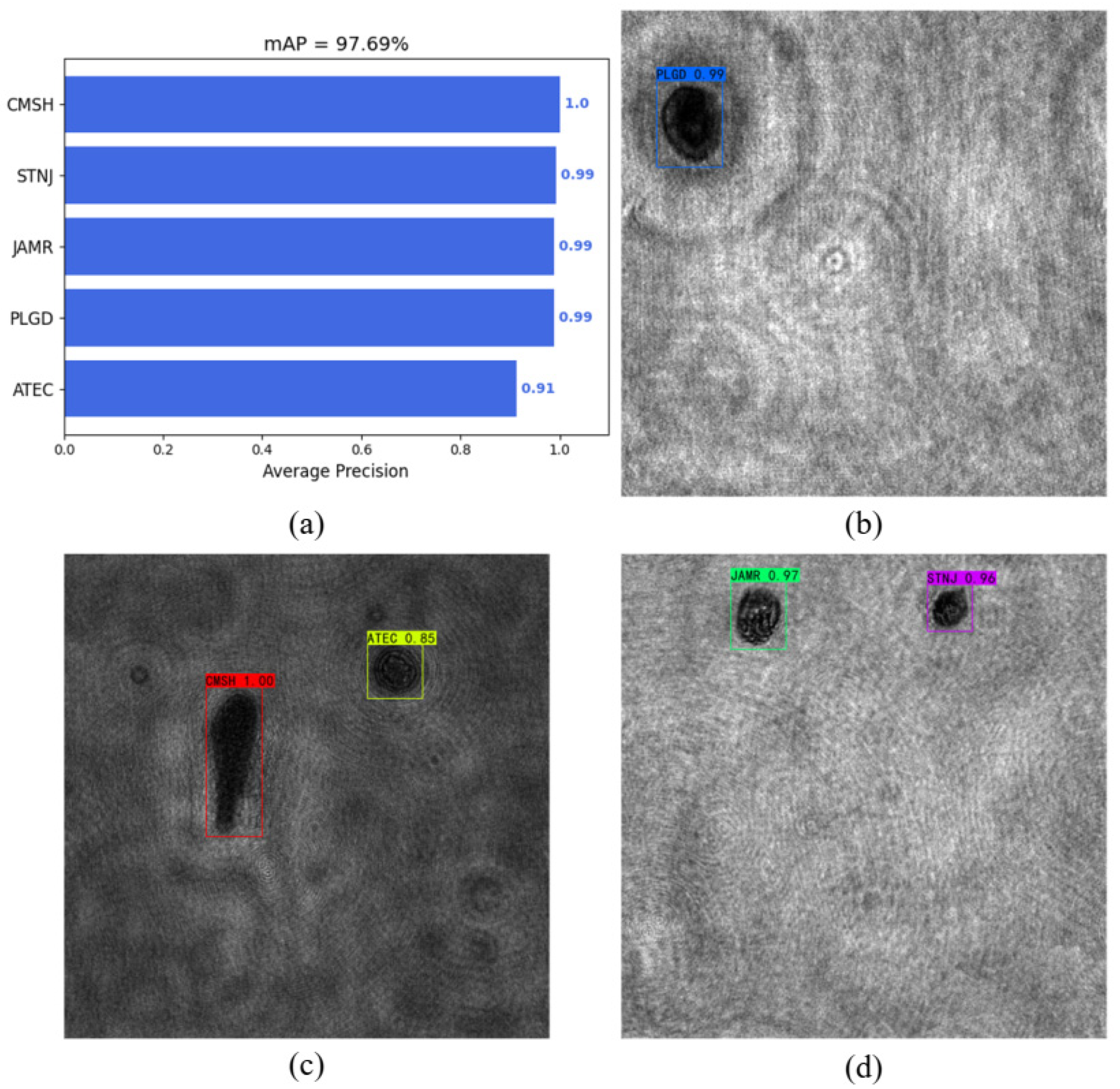
The results of the plankton detection are shown in Table 4. The mAP of the test dataset was 97.69%, and the results of plankton detection are shown in Figure 8.
During the hologram processing, the intensity of the reconstructed images varied with the reconstructed distance. In this study, YOLOv4 was robust and efficient for images with different contrasts and intensities.
5. Conclusions
The characteristics of a large depth of field imaging make it possible to detect a certain thickness of water at one time with DHM. However, the current detection methods discard the 3D information of holographic imaging, which can only identify the species and detect the concentration of plankton.
This paper presents a rapid plankton detection method that uses digital holographic imaging technology. During hologram processing, reconstructed hologram fusion is vital. A rapid image fusion method, ‘DHM-FCN’, was proposed to fuse the reconstructed images, which would suppress the background noise, the speckle noise inside the plankton, and the diffraction fringes around the plankton cell. DHM-FCN obtains the continuous edge of plankton cells. The fusion weight matrix could also be obtained from DHM-FCN. According to the weight value of every pixel, two reconstructed holograms would be fused to an image that contains all the focused plankton in the imaged water body. The fusion image is a two-dimensional representation of the three-dimensional imaged water body. The speed of DHM-FCN was 20 times faster than the WT fusion method, and the fusion performance was greatly improved. This makes it possible to quickly and accurately detect plankton in the field. DHM-FCN preserves detailed information about plankton and provides a good basis for the classification of plankton. YOLOv4 was applied to detect the five kinds of plankton with 97.69% mAP. The positions of plankton in the Z-axis and XY plane were obtained by focus distance and YOLOv4, respectively. The sizes of the cells were evaluated via the bounding box of the detector and the optical system parameters. The plankton detection method could locate and classify all plankton in the water body rapidly. Rather than obtaining information only on the categories and density of plankton, this method can be used to visualize the water more directly. Overall, the present study opens a new avenue for monitoring plankton in situ that involves the application of digital holographic microscopy.
Regarding future work, the use of YOLOv4 could be extended by using a greater number of species and samples. It is hoped that ocean experiments can be performed to improve the accuracy and feasibility of the algorithm.
Author Contributions
Conceptualization, K.L. and X.W.; methodology, K.L.; software, K.L. and H.C.; validation, K.L., H.C. and X.W.; formal analysis, K.L.; investigation, K.L.; resources, X.W.; data curation, K.L.; writing—original draft preparation, K.L.; writing—review and editing, K.L. and X.W.; visualization, K.L.; supervision, X.W.; project administration, X.W.; funding acquisition, X.W.; All authors have read and agreed to the published version of the manuscript.
Funding
National Natural Science Foundation of China (52171340); Key Science and Technology Project of Hainan Province, China (ZDYF2021SHFZ266).
Institutional Review Board Statement
Not applicable.
Informed Consent Statement
Not applicable.
Data Availability Statement
Not applicable.
Acknowledgments
We sincerely thank Meng-Meng Tong and her students for cultivating and providing all the plankton we used in this paper. We also thank Shihan Shan for providing relevant technical supports. Thank Lei Xu and Ke Chen for the optical system design.
Conflicts of Interest
The authors declare no conflict of interest.
References
- Bartley, T.; Mccann, K.S.; Bieg, C.; Cazelles, K.; Mcmeans, B.C. Food web rewiring in a changing world. Nat. Ecol. Evol. 2019, 3, 345–354. [Google Scholar] [CrossRef] [PubMed]
- Falkowski, P. Ocean Science: The power of plankton. Nature 2012, 483, 17–20. [Google Scholar] [CrossRef] [PubMed]
- Xu, F.L.; Tao, S.; Dawson, R.W.; Li, P.G.; Cao, J. Lake Ecosystem Health Assessment: Indicators and Methods. Water Res. 2001, 35, 3157–3167. [Google Scholar] [CrossRef]
- Hansen, P.J.; Moldrup, M.; Tarangkoon, W.; Garcia-Cuetos, L.; Moestrup, Ø. Direct evidence for symbiont sequestration in the marine red tide ciliate Mesodinium rubrum. Aquat. Microb. Ecol. 2012, 66, 63–75. [Google Scholar] [CrossRef] [Green Version]
- Onitsuka, G.; Yamaguchi, M.; Sakamoto, S.; Shikata, T.; Yamashita, H. Interannual variations in abundance and distribution of Chattonella cysts, and the relationship to population dynamics of vegetative cells in the Yatsushiro Sea, Japan. Harmful Algae 2020, 96, 101833. [Google Scholar] [CrossRef]
- Li, Y.; Zhao, Z.; Han, S.; Wang, X.; Liu, Z. Lagoon water quality monitoring based on digital image analysis and machine learning estimators. Water Res. 2020, 172, 115471. [Google Scholar] [CrossRef]
- Merz, E.; Kozakiewicz, T.; Reyes, M.; Ebi, C.; Isles, P.; Baity-Jesi, M.; Roberts, P.; Jaffe, J.S.; Dennis, S.; Hardeman, T. Underwater dual-magnification imaging for automated lake plankton monitoring. Water Res. 2021, 203, 117524. [Google Scholar] [CrossRef]
- Mes, A.; Ne, A.; Neg, B.; Mfa, C.; Ks, C.; Ba, D. Convolutional neural network—Support vector machine based approach for classification of cyanobacteria and chlorophyta microalgae groups. Algal Res. 2022, 61, 102568. [Google Scholar]
- Alvarez, E. Application of FlowCAM for phytoplankton enumeration, identification and estimation of chlorophyll content per cell. In Proceedings of the British Phycological Society 64th Annual Meeting, Bournemouth, UK, 23 June 2016. [Google Scholar]
- Kydd, J.; Rajakaruna, H.; Briski, E.; Bailey, S. Examination of a high resolution laser optical plankton counter and FlowCAM for measuring plankton concentration and size. J. Sea Res. 2017, 133, 2–10. [Google Scholar] [CrossRef] [Green Version]
- Otalora, P.; Guzman, J.L.; Acien, F.G.; Berenguel, M.; Reul, A. Microalgae classification based on machine learning techniques. Algal Res. 2021, 55, 102256. [Google Scholar] [CrossRef]
- Lefevre, F.; Chalifour, A.; Yu, L.; Chodavarapu, V.; Juneau, P.; Izquierdo, R. Algal fluorescence sensor integrated into a microfluidic chip for water pollutant detection. Lab Chip 2012, 12, 787–793. [Google Scholar] [CrossRef] [PubMed]
- Pinto, A.; Sperling, E.V.; Moreira, R.M. Chlorophyll—A Determination via continuous measurement of plankton fluorescence: Methodology Development. Water Res. 2001, 35, 3977–3981. [Google Scholar] [CrossRef]
- Pfitsch, D.W.; Malkiel, E.; Ronzhes, Y.; King, S.R.; Katz, J. Development of a free-drifting submersible digital holographic imaging system. In Proceedings of the Oceans, Washington, DC, USA, 17–23 September 2005. [Google Scholar]
- Monaldi, A.C.; Romero, G.G.; Alanís, E.; Cabrera, C.M. Digital holographic microscopy for microalgae biovolume assessment. Opt. Commun. 2015, 336, 255–261. [Google Scholar] [CrossRef]
- Talapatra, S.; Hong, J.; Mcfarland, M.; Nayak, A.R.; Zhang, C.; Katz, J.; Sullivan, J.; Twardowski, M.; Rines, J.; Donaghay, P. Characterization of biophysical interactions in the water column using in situ digital holography. Mar. Ecol. Prog. Ser. 2013, 473, 9–51. [Google Scholar] [CrossRef] [Green Version]
- Amolins, K.; Yun, Z.; Dare, P. Wavelet based image fusion techniques—An introduction, review and comparison. Isprs J. Photogramm. Remote Sens. 2007, 62, 249–263. [Google Scholar] [CrossRef]
- Pei, Y.; Zhou, H.; Jiang, Y.; Cai, G. The improved wavelet transform based image fusion algorithm and the quality assessment. In Proceedings of the 2010 3rd International Congress on Image and Signal Processing, Yantai, China, 16–18 October 2010. [Google Scholar]
- Pradnya, P.M.; Sachin, D.R. Wavelet based image fusion techniques. In Proceedings of the 2013 International Conference on Intelligent Systems & Signal Processing, Vallabh Vidyanagar, India, 1–2 March 2013; pp. 77–81. [Google Scholar]
- Long, J.; Shelhamer, E.; Darrell, T. Fully Convolutional Networks for Semantic Segmentation. IEEE Trans. Pattern Anal. Mach. Intell. 2015, 39, 640–651. [Google Scholar]
- Bochkovskiy, A.; Wang, C.Y.; Liao, H. YOLOv4: Optimal Speed and Accuracy of Object Detection. arXiv 2020, arXiv:2004.10934. [Google Scholar]
- Nicola, S.D.; Finizio, A.; Pierattini, G.; Ferraro, P.; Alfieri, D. Angular spectrum method with correction of anamorphism for numerical reconstruction of digital holograms on tilted planes. Opt. Express 2005, 13, 9935–9940. [Google Scholar] [CrossRef]
- Weng, J.; Zhong, J.; Hu, C. Digital reconstruction based on angular spectrum diffraction with the ridge of wavelet transform in holographic phase-contrast microscopy. Opt. Express 2008, 16, 21971–21981. [Google Scholar] [CrossRef]
- Likas, A.; Vlassis, N.; Verbeek, J.J. The Global K-Means Clustering Algorithm. Pattern Recognit. 2002, 36, 451–461. [Google Scholar] [CrossRef] [Green Version]
- Li, W.; Zhu, X.F. A new image fusion algorithm based on wavelet packet analysis and PCNN. In Proceedings of the International Conference on Machine Learning & Cybernetics, Guangzhou, China, 18–21 August 2005. [Google Scholar]
- Wu, J.P.; Yang, Z.X.; Su, Y.T.; Chen, Y.; Wang, Z.M. Wavelet transform and fuzzy reasoning based image fusion algorithm. In Proceedings of the International Conference on Wavelet Analysis & Pattern Recognition, Beijing, China, 2–4 November 2007. [Google Scholar]
- Qu, X.; Hu, C.; Yan, J. Image fusion algorithm based on orientation information motivated Pulse Coupled Neural Networks. In Proceedings of the World Congress on Intelligent Control & Automation, Chongqing, China, 25–27 June 2008. [Google Scholar]
- Liu, W.; Anguelov, D.; Erhan, D.; Szegedy, C.; Reed, S.; Fu, C.Y.; Berg, A.C. SSD: Single Shot MultiBox Detector. In European conference on computer vision; Springer: Berlin/Heidelberg, Germany, 2016; pp. 21–37. [Google Scholar]
- Ren, S.; He, K.; Girshick, R.; Sun, J. Faster R-CNN: Towards Real-Time Object Detection with Region Proposal Networks. IEEE Trans. Pattern Anal. Mach. Intell. 2017, 39, 1137–1149. [Google Scholar] [CrossRef] [PubMed] [Green Version]
- Girshick, R.; Donahue, J.; Darrell, T.; Malik, J. Rich Feature Hierarchies for Accurate Object Detection and Semantic Segmentation. In Proceedings of the IEEE Conference on Computer Vision and Pattern Recognition, Columbus, OH, USA, 23–28 June 2014; pp. 580–587. [Google Scholar]
- He, K.; Zhang, X.; Ren, S.; Sun, J. Spatial Pyramid Pooling in Deep Convolutional Networks for Visual Recognition. IEEE Trans. Pattern Anal. Mach. Intell. 2014, 37, 1904–1916. [Google Scholar] [CrossRef] [PubMed] [Green Version]
- Girshick, R. Fast R-CNN. In Proceedings of the IEEE International Conference on Computer Vision, Santiago, Chile, 7–13 December 2015; pp. 1440–1448. [Google Scholar]
- Redmon, J.; Divvala, S.; Girshick, R.; Farhadi, A. You Only Look Once: Unified, Real-Time Object Detection. In Proceedings of the IEEE Conference on Computer Vision and Pattern Recognition, Las Vegas, NV, USA, 27–30 June 2016. [Google Scholar]
- Redmon, J.; Farhadi, A. YOLO9000: Better, Faster, Stronger. In Proceedings of the IEEE Conference on Computer Vision and Pattern Recognition, Honolulu, HI, USA, 21–26 July 2017; pp. 6517–6525. [Google Scholar]
- Redmon, J.; Farhadi, A. YOLOv3: An Incremental Improvement. arXiv 2018, arXiv:1804.02767. [Google Scholar]
- Jia, D.; Wei, D.; Socher, R.; Li, L.J.; Kai, L.; Li, F.F. ImageNet: A large-scale hierarchical image database. In Proceedings of the 2009 IEEE Conference on Computer Vision and Pattern Recognition, Miami, FL, USA, 20–25 June 2009; pp. 248–255. [Google Scholar]
- Lin, T.Y.; Maire, M.; Belongie, S.; Hays, J.; Zitnick, C.L. Microsoft COCO: Common Objects in Context. In European Conference on Computer Vision; Springer: Berlin/Heidelberg, Germany, 2014; pp. 740–755. [Google Scholar]
- Wang, C.Y.; Liao, H.; Wu, Y.H.; Chen, P.Y.; Yeh, I.H. CSPNet: A New Backbone that can Enhance Learning Capability of CNN. In Proceedings of the 2020 IEEE/CVF Conference on Computer Vision and Pattern Recognition Workshops (CVPRW), Seattle, WA, USA, 13–19 June 2020. [Google Scholar]
- Liu, S.; Qi, L.; Qin, H.; Shi, J.; Jia, J. Path Aggregation Network for Instance Segmentation. In Proceedings of the IEEE Conference on Computer Vision and Pattern Recognition, Salt Lake City, UT, USA, 18–23 June 2018. [Google Scholar]
Figure 1.
The procedures of plankton detection. In Step I, OP represents object plane, HP represents hologram plane, IP represents image plane, and FD represents focus distance. In Step II, the inputs of the model are the two reconstructed holograms; the output of the model is the label graph.
Figure 1.
The procedures of plankton detection. In Step I, OP represents object plane, HP represents hologram plane, IP represents image plane, and FD represents focus distance. In Step II, the inputs of the model are the two reconstructed holograms; the output of the model is the label graph.

Figure 2.
(a) Diagram of the DHM optical system. (b) The setup of the experimental device.

Figure 3.
The holograms of the five plankton species. (a) The hologram of ATEC. (b) The hologram of CMSH. (c) The hologram of JAMR. (d) The hologram of PLGD. (e) The hologram of STNJ.
Figure 3.
The holograms of the five plankton species. (a) The hologram of ATEC. (b) The hologram of CMSH. (c) The hologram of JAMR. (d) The hologram of PLGD. (e) The hologram of STNJ.

Figure 4.
Reconstructed holograms (a), original hologram (b), and (c) reconstructed holograms with different focus distances.
Figure 4.
Reconstructed holograms (a), original hologram (b), and (c) reconstructed holograms with different focus distances.

Figure 5.
Visual representation of the weight matrix obtained from DHM-FCN.

Figure 6.
The results of different image fusion methods. (a) Result of PCNN, (b) result of RW, (c) result of PW, and (d) result of DHM-FCN.
Figure 6.
The results of different image fusion methods. (a) Result of PCNN, (b) result of RW, (c) result of PW, and (d) result of DHM-FCN.

Figure 7.
The relationship between the number of prior bounding boxes and accuracy.

Figure 8.
The results of YOLOv4, (a) mAP of YOLOv4, (b) the detection of PLGD, (c) the detection of CMSH and ATEC, and (d) the detection of JAMR and STNJ.
Figure 8.
The results of YOLOv4, (a) mAP of YOLOv4, (b) the detection of PLGD, (c) the detection of CMSH and ATEC, and (d) the detection of JAMR and STNJ.


Table 1.
Parameters of the traditional FCN model and the DHM-FCN model.
| Model | Size of the Parameter |
|---|---|
| FCN | 35,796,996 |
| DHM-FCN | 434,537 |
Table 2.
Structure of DHM-FCN model.
| Input | Layer | Stride | Output |
|---|---|---|---|
| 512 × 512 × 2 | Conv 3 × 3, 8 | 1 | C1, 512 × 512 × 8 |
| C1 | Maxpool 2 × 2 | 2 | P1, 256 × 256 × 8 |
| P1 | Conv 3 × 3, 16 | 1 | C2, 256 × 256 × 16 |
| C2 | Maxpool 2 × 2 | 2 | P2, 128 × 128 × 16 |
| P2 | Conv 3 × 3, 32 | 1 | C3, 128 × 128 × 32 |
| C3 | Maxpool 2 × 2 | 2 | P3, 64 × 64 × 32 |
| P3 | Conv 3 × 3, 64 | 1 | C4, 64 × 64 × 64 |
| C4 | Maxpool 2 × 2 | 2 | P4, 32 × 32 × 64 |
| P4 | Conv 3 × 3, 128 | 1 | C5, 32 × 32 × 128 |
| C5 | Maxpool 2 × 2 | 2 | P5, 16 × 16 × 128 |
| P5 | Conv 1 × 1, 256 | 1 | C6, 16 × 16 × 256 |
| C6 | DeConv 4 × 4, 64 | 2 | D1, 32 × 32 × 64 |
| D1 & P4 | Skip | - | K1, 32 × 32 × 64 |
| K1 | DeConv 4 × 4, 32 | 2 | D2, 64 × 64 × 32 |
| D2 & P3 | Skip | - | K2, 64 × 64 × 32 |
| K2 | DeConv 16 × 16, 1 | 8 | D3, 512 × 512 × 1 |
Table 3.
Evaluation of indicators for image fusion methods.
| Method | Operation Time (s) | SSIM | Cor | PSNR |
|---|---|---|---|---|
| PCNN | 0.1786 | 0.5726 | 0.7998 | 71.7134 |
| RW | 0.7877 | 0.6387 | 0.8151 | 71.7115 |
| PW | 0.7334 | 0.6391 | 0.8153 | 71.7112 |
| DHM-FCN | 0.03395 | 0.7067 | 0.8782 | 74.2479 |
Table 4.
Detection effect of plankton.
| Species | Abbreviation | AP | Recall | F1 Score |
|---|---|---|---|---|
| Alexandrium tamarense | ATEC | 91.41 | 81.25 | 78 |
| Chattonella marina | CMSH | 100 | 100 | 98 |
| Mesodinium rubrum | JAMR | 98.91 | 97.78 | 92 |
| Scrippsiella trochoidea | STNJ | 99.25 | 100 | 97 |
| Prorocentrum lima | PLGD | 98.89 | 95.83 | 94 |
Publisher’s Note: MDPI stays neutral with regard to jurisdictional claims in published maps and institutional affiliations. |
© 2022 by the authors. Licensee MDPI, Basel, Switzerland. This article is an open access article distributed under the terms and conditions of the Creative Commons Attribution (CC BY) license (https://creativecommons.org/licenses/by/4.0/).
Share and Cite
MDPI and ACS Style
Lang, K.; Cai, H.; Wang, X. A Plankton Detection Method Based on Neural Networks and Digital Holographic Imaging. Chemosensors 2022, 10, 217. https://0-doi-org.brum.beds.ac.uk/10.3390/chemosensors10060217
AMA Style
Lang K, Cai H, Wang X. A Plankton Detection Method Based on Neural Networks and Digital Holographic Imaging. Chemosensors. 2022; 10(6):217. https://0-doi-org.brum.beds.ac.uk/10.3390/chemosensors10060217
Chicago/Turabian StyleLang, Kaiqi, Hui Cai, and Xiaoping Wang. 2022. "A Plankton Detection Method Based on Neural Networks and Digital Holographic Imaging" Chemosensors 10, no. 6: 217. https://0-doi-org.brum.beds.ac.uk/10.3390/chemosensors10060217
Note that from the first issue of 2016, this journal uses article numbers instead of page numbers. See further details here.