Classification of Aviation Alloys Using Laser-Induced Breakdown Spectroscopy Based on a WT-PSO-LSSVM Model

Abstract

It is well-known that aviation alloys of different grades show large differences in mechanical properties. At present, alloys must be strictly distinguished in the manufacturing plant because their close appearance and density are easily confused In this work, the wavelet transform (WT) method combined with the least squares support vector machine (LSSVM) is applied to the classification and identification of aviation alloys by laser-induced breakdown spectroscopy (LIBS). This experiment employed six different grades of aviation alloy as the classification samples and obtained 100 sets of spectral data for each sample. This research included the steps of preprocessing the obtained spectral data, model training, and parameter optimization. Finally, the accuracy of the training set was 99.98%, and the accuracy of the test set was 99.56%. Therefore, it is concluded that the model has superior generalization capacity and portability. The result of this work illustrates that LIBS technology can be adopted for the rapid identification of aviation alloys, which is of great significance for on-site quality control and efficiency improvement of aerospace parts manufacturing.

1. Introduction

In aero-engines, an increasing number of special materials are used to make blades and critical components [1]. These materials are called aerospace alloys, and are applied in different parts of an aero-engine. Although the materials of the blades at all levels of the aero-engine are different, the appearances of aviation alloys of some grades are similar. In avoiding the mixing of raw materials when the same production line produces blades of different materials, the rapid classification of aviation alloys is important. In general, multielement analysis of alloys can be performed in analytical laboratories, and can include inductively coupled plasma-mass spectrometry (ICP-MS) [2], X-ray fluorescence (XRF) [3], and flame atomic absorption spectrometry (AAS) [4]. However, traditional classification techniques usually require complex sample pretreatment processes, and they are significantly affected by the on-site environment. Moreover, the above traditional methods are not conducive to rapid analysis in the industrial field. Therefore, this study proposes a classification method for aviation alloys based on laser-induced breakdown spectroscopy (LIBS).

The principle of LIBS technology is presented as follows. When the laser emits a light pulse, the high-power pulsed laser beam is focused on the sample to be tested using a lens. The object to be tested is excited by ablation, and a plasma plume is instantly generated on its surface. Qualitative and quantitative analysis of the chemical composition is achieved by collecting wavelength and intensity information of the atomic and ionic spectra in the plasma. Some scholars also call it an “active sensor” [5] (laser-plasma emits radiation, the radiation can reflect information about the sample composition, and an optical spectrometer collects information about optical spectra). As a result, LIBS is widely used to explore chemical composition in the industry [6,7,8], space [9,10], underwater [11,12], and geology [13,14] fields, among others. Our research group [15,16,17] also conducted related research on long–short double-pulse laser-induced breakdown spectroscopy technology, and performed a quantitative analysis of steel. LIBS has the advantages of a wide range of analyzable elements, low requirements for the preparation of the substances to be tested, rapid real-time online detection, and high accuracy of quantitative analysis. Therefore, LIBS technology has the potential to rapidly analyze aviation alloys. However, alloys and other raw materials of different grades have the same appearance characteristics and the same main elements. Only the trace element content is different. In addition, the direct use of LIBS to measure the content of trace elements has high requirements for the accuracy and repeatability of the measurement.

In recent years, some researchers have combined LIBS with machine learning for material classification to achieve remarkable classification results. Zhan et al. [18] proposed a fast classification method for aluminum alloys using LIBS and RF (random forest) algorithms. Further, they revealed the law that the accuracy varies with the number of trees in the RF and the size of the training sample set. Liang et al. [19] reported a steel multiclassification method based on a support vector machine. However, the robustness of using full-spectrum data is insufficient, and the amount of calculation required is extremely large. Campanella et al. [20] proposed a classification strategy for light alloys. They believe that the evaluation method for aluminum scrap sample classification by artificial neural network and LIBS technology is effective. Lin et al. [21] employed partial least squares discriminant analysis (PLS-DA) and support vector machine (SVM) to study 40 kinds of steel, with accuracy of 96.25% and 95%, respectively.

However, the above methods still have certain limitations, including the sensitivity of the optical spectrometer, laser power radiation, the collection of the optical signal, the low level of trace elements, LIBS setup, etc. Meanwhile, the metal materials with similar chemical compositions have fewer differences in spectral lines, which is not conducive to classification and identification. Therefore, it is necessary to increase the front-end signal preprocessing for LIBS analysis. To overcome this problem, this work aimed to develop a LIBS method for the classification of aviation alloys. Based on a LIBS experimental setup, the spectral data were acquired from six samples with different grades. The wavelet transform was first adopted to extract features from spectral data. Subsequently, four machine learning models were established to classify and predict samples. Finally, three evaluation criteria (accuracy, precision, and sensitivity) for model performance were proposed. In other words, this issue will not only be an obstacle to training a model with strong prediction capability, but will also lead to poor model generalization ability for the classification of mixed aviation alloys.

2. Materials and Methods

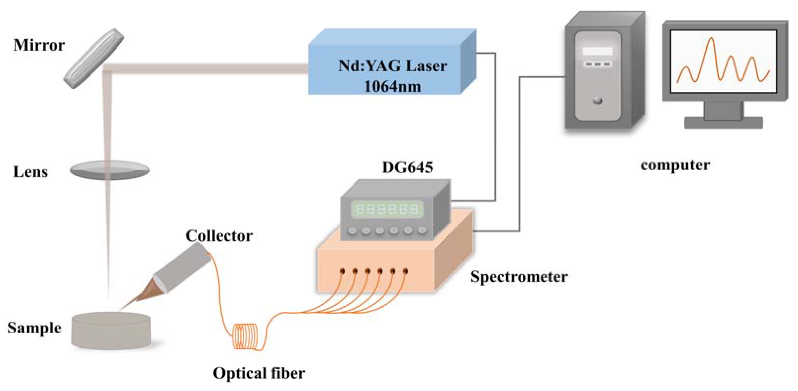
2.1. Experimental System

Figure 1 shows the schematic diagram of the LIBS system that was employed to measure the six aviation alloys in the current work. The pulsed laser beam is generated by an Nd: YAG solid-state laser (Dawa-300, Beamtech Optronics Co., Ltd., Beijing, China). In the Q-switched mode of the laser, the pulse width reaches 6 ns. In this experiment, the laser was operated at 1064 nm with a pulse energy of 50 mJ and a frequency of 10 Hz. The laser beam was reflected by a mirror and focused on the sample surface by a lens (f = 60 mm). The emission of the plasma plume was collected by a collimating lens (focal length 60 mm) at an angle of 45° to the incident laser, and transmitted through an optical fiber to a six-channel spectrometer (AvaSpec Multi-Channel, Avantes, Amsterdam, Holland). The range of the spectrometer is 220–880 nm, and the resolution is 0.08–0.11 nm. The trigger timing between the devices was controlled by a delay generator (DG645, Standford Research Systems, Stanford, CA, USA). The delay time between the laser pulse and the spectrometer signal acquisition was 300 ns.

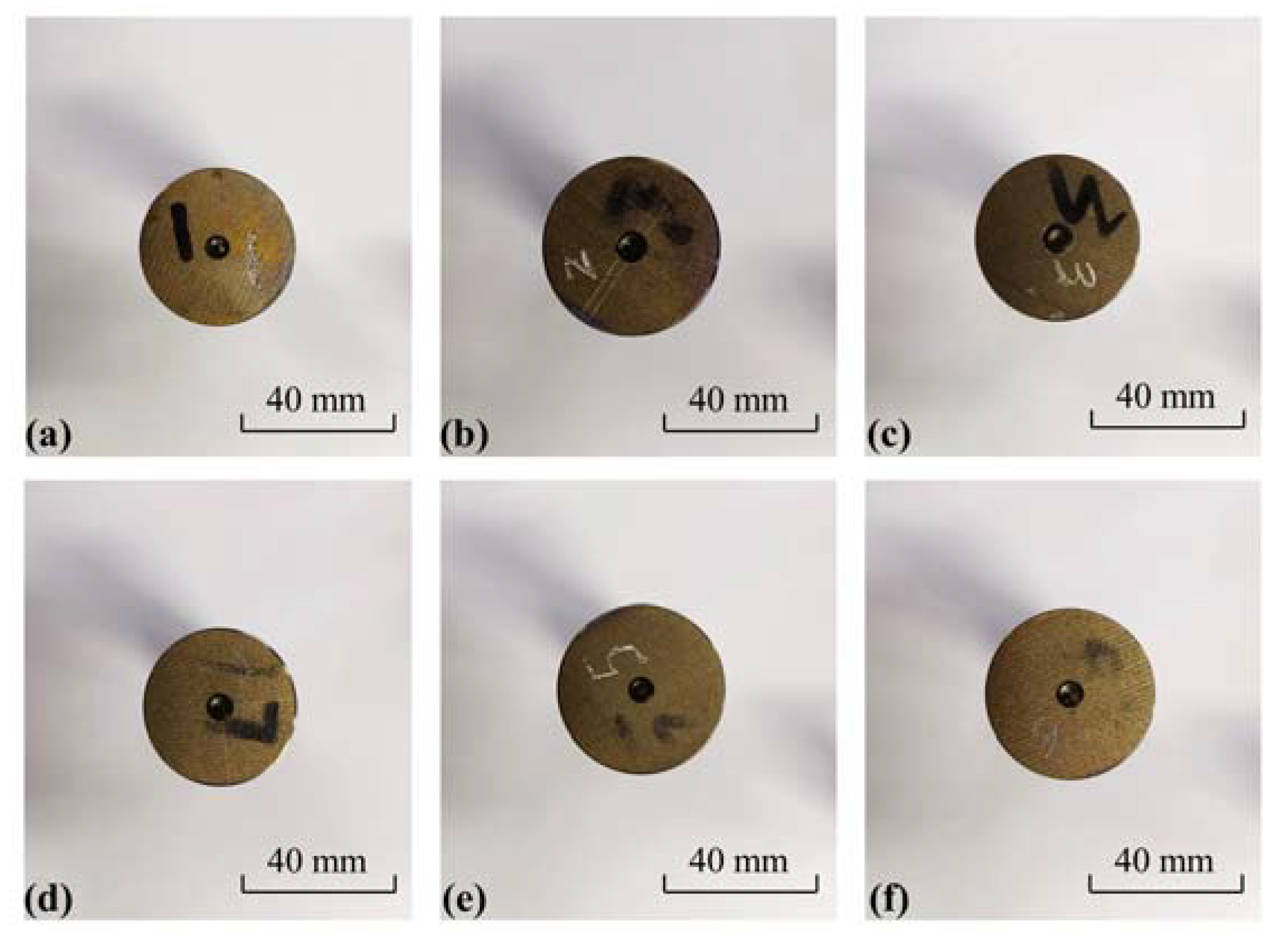
2.2. Sample and Spectral

Figure 2 presents the physical picture for six samples with different grades: 42CrMo, A100, GH4169, TC4, TC11, and TC17. The sample concentration in

Table 1. Concentration information of examined elements in six aviation alloy samples.

No.	Sample Name	Composition (wt%)
		Cr	Ni	Si	Mn	Mo	Al	Fe	other
1	GH4169	19.01	52.30	0.05	0.03	3.06	0.57	18.83	6.15
2	42CrMo	0.90	-	0.17	0.50	0.15	-	97.90	0.38
3	A100	2.90	11.00	0.10	0.10	1.10	0.015	60.76	24.03
		Zn	Al	Mo	Fe	Zr	Si	Ti	other
4	TC4	-	5.50	-	0.50	-	-	90.15	3.85
5	TC11	1.40	5.80	2.80	0.25	0.80	0.02	87.73	1.20
6	TC17	1.90	-	3.90	0.06	1.90	-	88.44	3.80

was measured by the spark-optical emission spectroscopy method. A standard spark emission spectrometer (ARL4460, Thermo Fisher Scientific Co. Ltd., Waltham, MA, USA) was employed to measure the elemental contents in each sample. The measurement parameters were selected as follows. Light source: low-pressure spark, voltage: 230 V, pre-ablation time: 12 s, and exposure time: 4 s. For instance, the content of Ni in GH4169 was high, and it was low in 42CrMo. The content of Mo in TC17 was high, and it was low in TC4. This means that the differences in the composition of the aviation alloys themselves make the classification possible. Because the first three samples and the last three samples are chemically similar, so we divided them into two groups to show their chemical composition distinctly.

To simulate a real industrial environment, this work did not perform any preprocessing work on the samples, nor did it actively control the movement of the samples. Currently, data preprocessing techniques cannot effectively eliminate spectral differences caused by compositional inhomogeneity. More measurement locations are required to obtain sufficient spectral information concerning compositional variability. Therefore, under the same experimental conditions, according to the average results of 10 laser pulses, 20 laser pulses, and 100 laser pulses, 100 sets of spectral data were measured for different positions at each sample. The first 20 excitations at each location were employed to clean the surface impurities. Finally, a total of 1800 sets of spectral data were obtained. Not only were they extremely similar in appearance and spectral information, but they also did not exhibit any features that could be adopted for classification and identification. Due to the complexity and similarity of these samples, a set of characteristic spectral lines needed to be extracted to maintain the reliability of the discrimination.

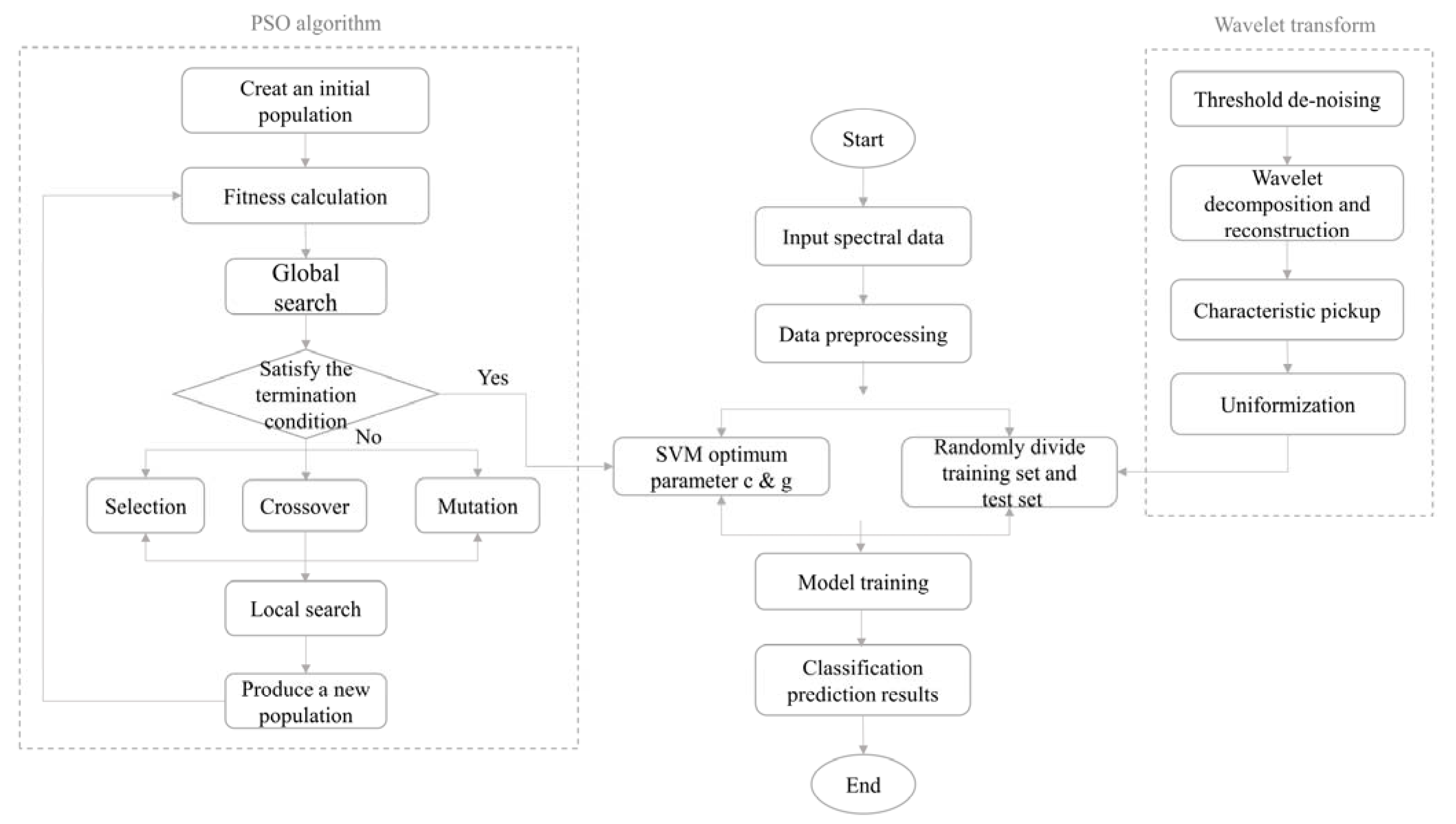
2.3. Algorithm Discrimination

In the current work, the research framework was mainly divided into three parts: spectral data preprocessing, model parameter optimization, model training, and classification prediction, as shown in Figure 3.

Initially, threshold noise reduction was used to remove complex and redundant data. Wavelet decomposition and reconstruction were employed to lower the dimension of high-dimensional data to select eigenvalues. As 42CrMo, A100, and GH4169 were steel and superalloy series, with TC4, TC11, and TC17 being a titanium alloy series, as shown in Table 1, they were divided into two groups for the classification test, and the “db4” result was input into the model as a feature set. In order to test the performance of the classification model, two groups of each sample were selected randomly.

Then, the normalized data were input into the model as a dataset for training. Secondly, model parameters were optimized using particle swarm optimization. After a series of operations, such as population initialization, fitness calculation, and global search, the result was judged on whether it satisfied the termination condition. If the conditions were satisfied, the optimal parameters were input into the model. If not, the selection, crossover, and mutation continued to generate a new iteration. Finally, the support vector machine learning method was adopted, entering the optimized parameters c (penalty coefficient) and g (kernel parameter).

2.3.1. Support Vector Machines (SVM)

Support vector machines were proposed by Vapnik & Corts [22] in the mid-1990s. They are a machine learning method based on statistical learning theory, or VC theory, which is defined as the maximum number of points that the classifier can disperse, and the principle of structural risk minimization. SVM exhibits many unique advantages in solving small-sample, nonlinear, and high-dimensional pattern recognition problems, and overcomes the “curse of dimensionality” to a large extent. It has been extensively applied in function estimation, time series forecasting, and pattern recognition, as well as other fields. The determinant function and the decision function of the hyper-plane are expressed as follows [23]:

$$f(z)=sign({\displaystyle \sum _{i=1}^n{\lambda }_i{y}_{i}K(x_i,z)+b})$$

(1)

$$y(x)=sign\left[{\displaystyle \sum _{k=1}^N{\alpha }_k{y}_k\psi (x,x_k)+b}\right]$$

(2)

Given a training set of data points ${\left\{{\mathrm{y}}_k,x_k\right\}}_{k=1}^N$, where $x_i$ represents the input spectrum containing $d$ variables, $y_i$ is the class label (kinds of aviation alloys) indicating the class to which the point $x_i$ belongs, ${\lambda }_i$ stands for the Lagrange multiplier, $K\left(x_i,z\right)$ is the kernel function, $z$ is the spectrum from the unknown sample, and $b$ denotes the mean value of the offset.

As a general learning machine, it essentially solves the convex quadratic programming problem. Since the principle of structural risk minimization is employed to control both the empirical risk and the complexity of the learning machine, the phenomenon of over-learning can be effectively avoided. In addition, better generalization ability can be obtained than the traditional learning method.

The kernel function can transform the original nonlinear problem into a linear problem in a high-dimensional space. Through the mapping function, the original feature space is mapped to a higher-dimensional space. Moreover, the data that are inseparable in the original space may become linearly separable in the high-dimensional space. Common kernel functions include the linear kernel, polynomial kernel, radial basis function, and sigmoid kernel. In the present study, prior knowledge was used to select the RBF kernel function [24].

However, the classic SVM model is more complex, and the solution speed is slower. The least squares support vector machine is an improvement to the classical support vector machine. It solves a set of linear equations instead of the complicated quadratic optimization problem in the classical SVM, which can efficiently reduce the computational complexity and speed up the computation.

2.3.2. Least Squares Support Vector Machine (LSSVM)

The least squares support vector machine proposed by Suykens [25] et al. in 1999 is an improved support vector machine based on statistical theory. It can transform the solution of a quadratic optimization problem into the solution of a linear equation system, which can simplify the solution of the problem.

LSSVM is used as the loss function. The solution process refers to the understanding of an equation system, and the solution speed is relatively fast. It is applied to pattern recognition and nonlinear function estimation and has generated good results. Its key parameters are the parameters in the kernel function, and the regularization parameters are collectively referred to as hyperparameters. In the meantime, the inequality constraint problem in the classical SVM algorithm is transformed into an equality constraint problem, which can significantly reduce the difficulty of solving the problem.

3. Results and Discussion

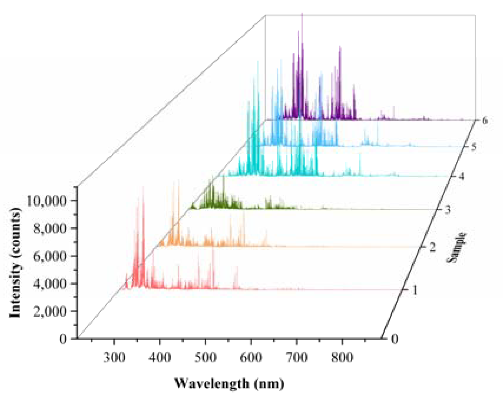
3.1. Data Acquisition

As shown in Figure 4, the range with more emission lines was between 200 nm~550 nm. The intensity was weak in the range above the wavelength of 550 nm. However, due to many spectral lines, the workload was greatly increased when all were selected. As a result, it was necessary to filter them to select the most representative spectral lines as the characteristic lines for performing the subsequent analysis. For each of the alloy samples, the performance of the classification model was evaluated using 210 sets of spectra as training sets and 90 sets of spectra as test sets. The specific label information of the samples is displayed in the first column of Table 1. The data we obtained had a total of 12,565 spectral points, and each data point contained information about the type of aviation alloy sample, but a large quantity of data can make calculations difficult. It was necessary to appropriately reduce the dimensionality of the data.

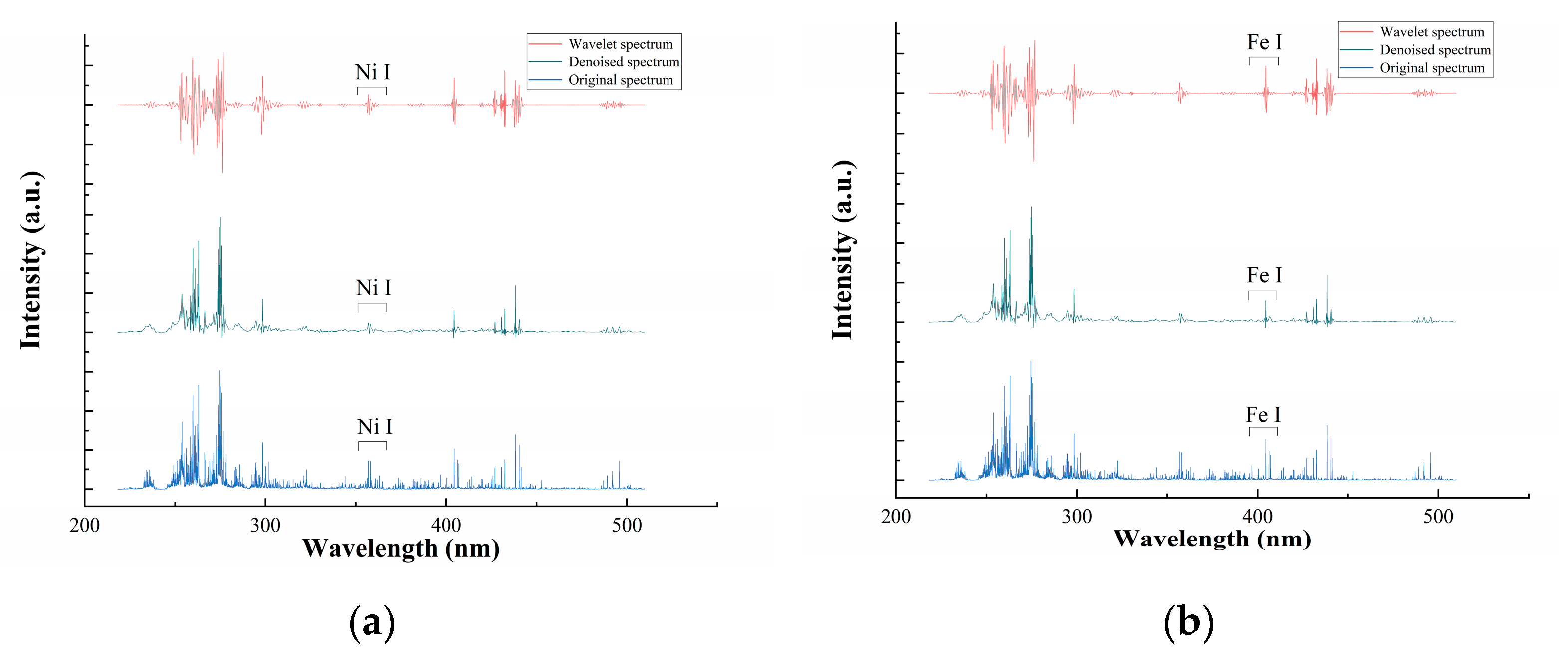
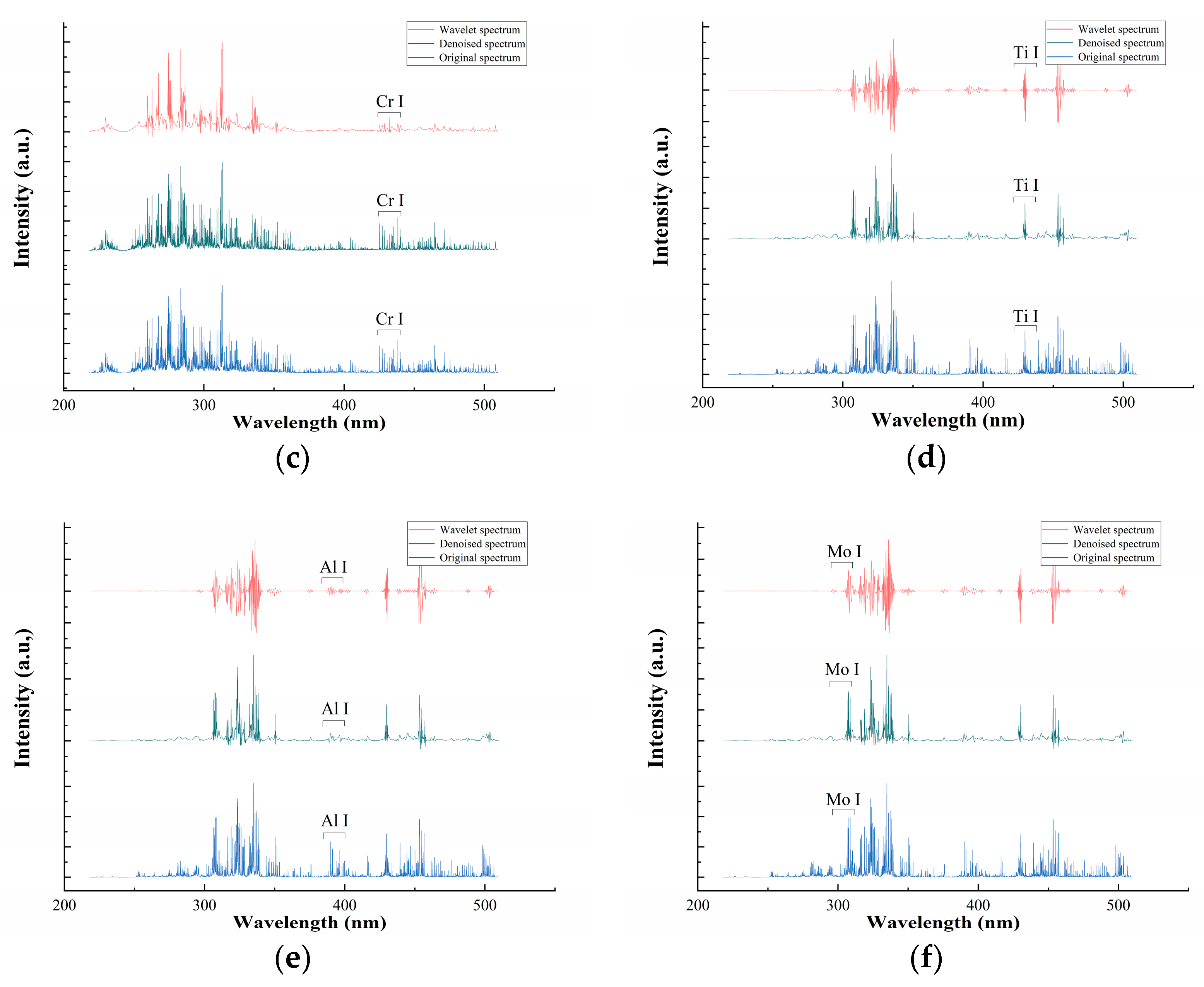
3.2. Spectral Data Pretreatment

The interference of random noise in the field environment, continuous background, and impurity elements on the sample surface can cause serious spectral background, low signal-to-noise ratio, and poor spectral stability. High-dimensional spectral data and relatively small sample sizes can make it challenging to map measured variables to dependent variables. In other words, the performance of multivariate models can be influenced by redundant variables (such as noise) and interfering variables (such as background and spectral feature overlap) throughout the spectrum [26]. The existence of these shortcomings leads to the low detection accuracy of LIBS, which could hinder its further development in engineering applications.

In addition, due to the high cost of improving experimental conditions and investment as well as the limited improvement effect, it is more convenient and efficient to adopt data processing methods. A common preprocessing process consists of spectral noise reduction [27], baseline correction [28], spectral overlapping peak resolution [29] and data compression [30]. Spectral data processing can improve the signal-to-noise ratio (SNR) of the signal, but it can also lower the fluctuation of the signal, thereby improving the detection sensitivity, stability, and reproducibility of LIBS. According to Zou’s [27] study, wavelet preprocessing can effectively improve the quality of the signals and the accuracy of the regression model. This method has already been used as a competitive preprocessing tool for LIBS and other spectral analyses. Wavelet transform is a mathematical function that is generally used to divide a given continuous-time signal into different components with multiscale and multiresolution conditions. From another point of view, the role of WT is equivalent to eliminating the matrix effect and improving the self-absorption effect of the LIBS spectrum.

In this work, to avoid the phenomenon of signal oscillation and pseudo-Gibbs, the experiment firstly performed threshold noise reduction on the signal after the original spectrum acquisition and noise analysis by the Birge–Massart strategy. The method has been confirmed as having superior adaptability and is extensively applied in signal and image processing [31,32]. The original LIBS data were subsequently compressed and decomposed by the method of wavelet transform (WT). This study used “db4” [33] (the “db” refers to a particular family of wavelets) to reconstruct the four-layer wavelet coefficients. The spectral line signals after feature extraction of the six samples are displayed in Figure 5. The bottom layer was the original spectral line, the middle layer was the spectral line after noise reduction, and the top layer was the spectral line after wavelet feature extraction. This reveals that WT pretreatment retains the detailed characteristic emission lines, smoothing the noise signal perfectly. At the same time, it indicates almost all the selected features are peaks and wavelengths around the peaks. The result is consistent with the expectation that the emission peak region in the LIBS data contains more valuable spectral information.

From the National Institute of Standards and Technology (NIST) database, the main lines of the alloying elements and impurity elements of the six aviation alloy materials were selected in

Table 2. Selection of characteristic spectral lines [34].

Significant Element	Main Wavelength (nm)
Ni I	352.454
Fe I	357.199 373.486 404.581 438.354
Cr I	425.435 427.480 428.972
Ti I	468.19 498.173
Al I	309.27 396.152
Mo I	313.259 550.649

such as Ni (Nickel), Fe (Iron), Cr (Chromium), Ti (Titanium), Al (Aluminum), and Mo (Molybdenum). As shown in Figure 5, the intensity of the Ni element excited in GH4169 is much larger than that of the Ni element excited in 42CrMo, the intensity of the Al element excited in TC 11 is much larger than that of the Al element excited in TC 17. By observing the waveforms after preprocessing, it was not difficult to find that the main chemical composition lines of each material are preserved. These results demonstrate that the method of extracting spectral information by the algorithm is reliable and more efficient.

3.3. Calibration Model

3.3.1. Model Establishment

Figure 6 shows the classification results of three samples, TC4, TC11, and TC17. The x-axis represents the sample spectrum number (210 for training, 90 for model testing) and the y-axis represents the sample type. “o” denotes the actual label of each set of spectral data, and “*” stands for the predictive label. Coinciding the two indicates that the prediction was accurate. Conversely, it suggests that the prediction was not correctly identified. Figure 6a shows the result of the SVM model, which had poor prediction accuracy. Figure 6b presents the PSO-optimized SVM. The accuracy of predictions was improved, but it was still not at the ideal level. Figure 6c displays the result of LSSVM. The classification effect was significantly improved. As illustrated in Figure 6d, the classification prediction accuracy of the LSSVM model after parameter optimization was close to 100%, which was in line with the expected effect of the model. In the discriminant analysis, machine learning methods were applied to extract potential information and rules in the data instead of manually comparing the differences between two types of spectra, thereby greatly improving the accuracy of the classification analysis.

Theoretically, overfitting may occur due to the high-dimensional spatial characteristics of spectral data. Apart from that, the similarity of the composition of several alloy materials can hinder the classification accuracy and reduce the sensitivity. It is significant that support vector machines are more suitable for binary classification problems, but are less effective for multiclassification. Upon comparison of the recognition results of SVM and LSSVM, the accuracy of LSSVM was generally higher than that of SVM. The LSSVM model solves the sample size constraints and nonlinear problems in quadratic programming. Then, the influence of the matrix effect on the experimental results was largely eliminated. As a result, the computational efficiency and stability of the LSSVM classification model were higher than those of the support vector machine classification model for aviation alloys.

3.3.2. Parameter Optimization

The choice of parameters had a greater impact on the prediction results of the mixed classification model. Nowadays, there is no better parameter selection rule, as it has a certain blindness, while traditional models often use trial and error or ergodic optimization.

Particle swarm optimization (PSO) [35] is an evolutionary computing technology developed by Kennedy & Eberhart in 1995. It is derived from a simulation of a simplified social model. PSO has the advantages of not easily falling into local minima, being easy to implement, and having fewer parameters to adjust. In addition, it is used to handle nonlinear, non-differentiable, and multimodal problems. However, there are two keys to the application of PSO in selecting hyperparameters. One is the matter of how to represent the hyperparameters with particles, and the other is that of how to define the fitness function. They are defined as follows:

$$fitness=\frac{1}{MRE}$$

(3)

$$MRE=\frac{1}{N}{\displaystyle \sum _{i=1}^N\left|\frac{y_i-\widehat{y_i}}{y_i}\right|}\times 100\%$$

(4)

where $N$ is the number of samples in the test set, and $y_i$${\mathrm{y}}_i$ and $\widehat{y_i}$ represent the predicted and actual values, respectively. After obtaining the optimal hyperparameters, a machine learning model can be built with training data and prediction data.

In this study, the initialized learning factor was 1.5, the initial weight was 1.0, the termination weight was 0.6, the number of iterations was 100, and the fitness of each particle was 0.0389.

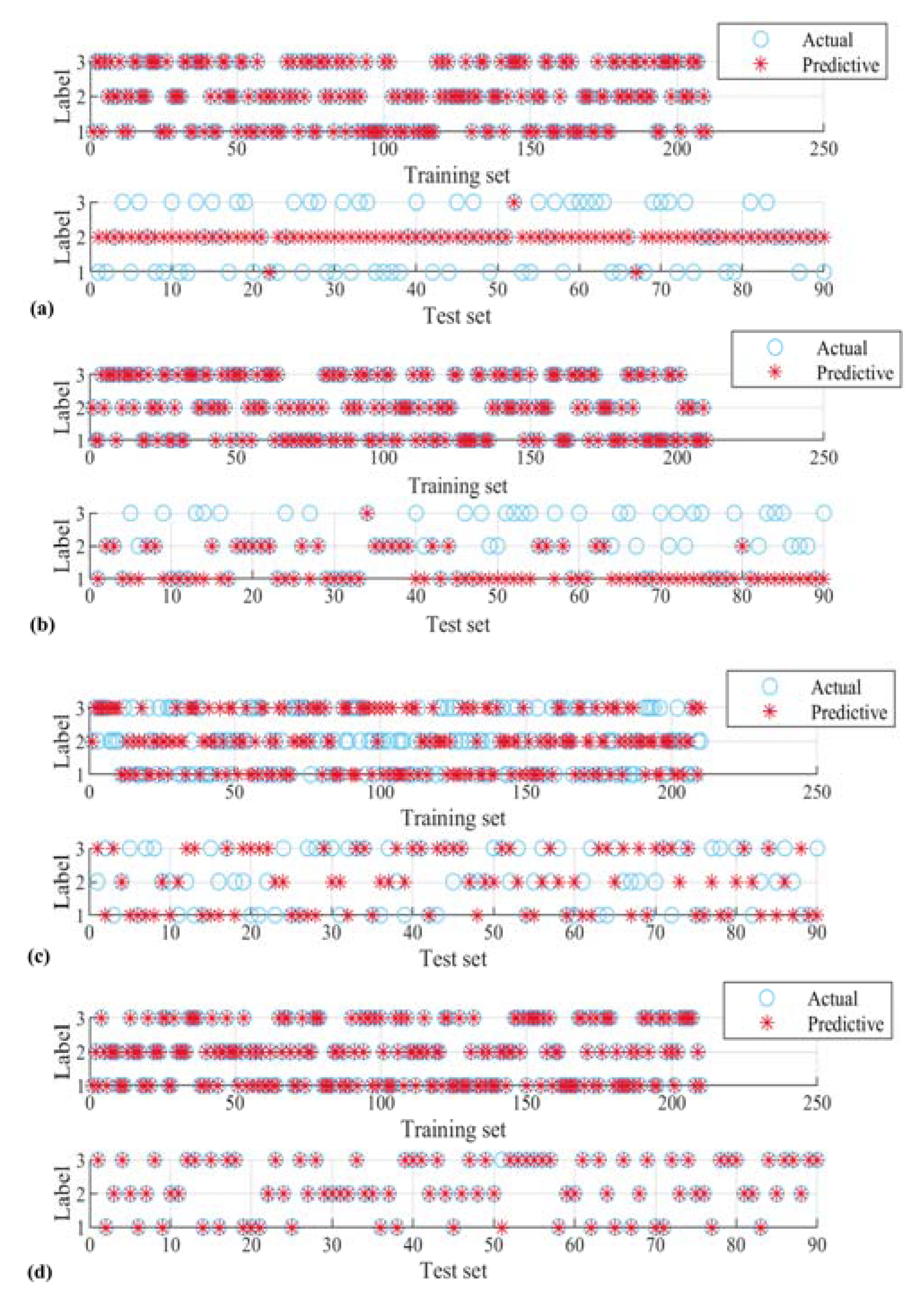
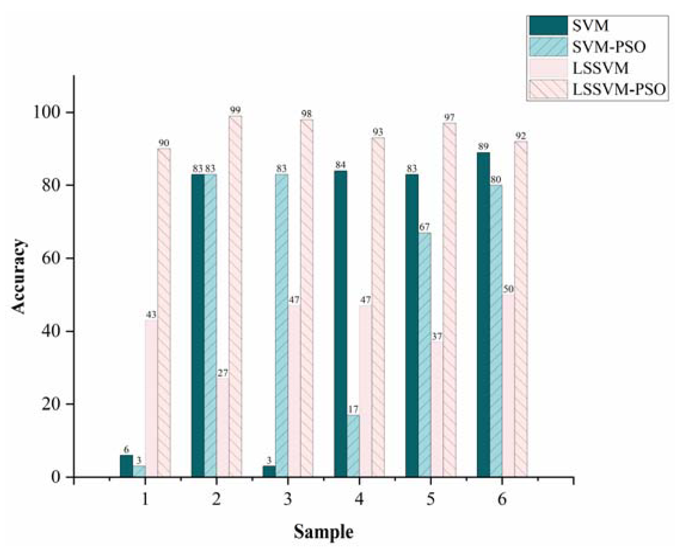
3.4. Model Evaluation

This work demonstrated the predictive performance of four classification models. Accuracy, precision, and sensitivity were the statistical parameters to evaluate these models. They were used as evaluation metrics for machine learning classification prediction, and they can be defined as follows:

$$Accuracy=\frac{TP+TN}{TP+TN+FP+FN}$$

(5)

$$Precision=\frac{TP}{TP+FP}$$

(6)

$$Sensitivity=\frac{TP}{TP+FN}$$

(7)

where $TP$, $FP$, $TN$, and $FN$ represent true positive, false positive, true negative, and false negative, respectively [35]. That is to say, accuracy describes the percentage of correct model classification, precision describes the degree of accuracy of the positive samples predicted by the model, and sensitivity describes the ability of the model to identify a positive sample from a true positive sample.

After the initial sample excitation, spectral data collection, and feature extraction, the performance of the machine learning model was evaluated from the three perspectives of accuracy, precision, and sensitivity. According to

Table 3. The predictive performance of four classification models.

Models	Accuracy (%)	Precision (%)	Sensitivity (%)
SVM	38.79	31.45	37.21
SVM–PSO	64.33	67.46	68.58
LSSVM	92.51	89.72	91.48
LSSVM–PSO	99.98	99.56	99.89

, the comparison of the classification results of the four models showed that the accuracy, precision, and sensitivity of the SVM model were lower than those of the other models. In addition, the classification performance and stability of the SVM–PSO model were also unsatisfactory due to the uneven surface of the sample, which was full of impurities with similarity to the titanium–aluminum alloy composition. Nonetheless, the better results also showed that our previous wavelet preprocessing algorithm had extracted effective dataset features.

As an improved SVM model, LSSVM can build linear and nonlinear modeling. This largely eliminated the influence of matrix effects on the experimental results, and it solved the classification problem of mixed samples satisfactorily. In addition, it was able to realize high-dimensional feature space learning in a small number of samples, and effectively avoided the problem of low classification accuracy caused by data overfitting. Thus, Figure 7 shows that along with the optimization and improvement of the model, the prediction accuracy of the test set was continuously improving. The results demonstrate that the WT–PSO–LSSVM model presented the best classification accuracy, precision, and sensitivity compared with the other methods. Compared with the original SVM classification model, this method not only takes the relationship between spectral intensity into better consideration, but also eliminates many redundant variables at the beginning for better construction of subsequent models. In contrast with traditional qualitative analysis methods that rely on element wavelength positions and corresponding spectral line intensities, the machine learning model exploits some comprehensive regularities for spectral analysis.

4. Conclusions

To conclude, although LIBS is an advanced detection technology, it was necessary to combine it with some algorithms to reach the goal of rapid and accurate classification. In the current work, LIBS, combined with the four machine learning models SMV, SVM–PSO, LSSVM, and LSSVM–PSO, was successfully applied to the classification of six aviation alloys. Afterward, considering that it is difficult to build a well-trained model directly based on high dimensional data, the preprocessing operation of front-end feature selection for spectral data by wavelet transform was proposed to mitigate the existing problem. The results demonstrate that the LSSVM–PSO model achieved the best performance, correctly identifying 100 groups of the spectra out of the total 300 groups. The accuracy, precision, and sensitivity used to evaluate the four models also exhibited the best performance in the LSSVM–PSO model. In addition, it was confirmed that the combination of LIBS technology and machine learning can be effectively used as a real-time, non-destructive, and multielement online analysis method for aviation alloy classification with broad application foreground.

References

1. Gialanella, S.; Malandruccolo, A. Aerospace Alloys, 1st ed.; Springer: Cham, Switzerland, 2020; pp. 14–15. [Google Scholar] [CrossRef]
2. Leach, A.M.; Hieftje, G.M. Identification of alloys using single shot laser ablation inductively coupled plasma time-of-flight mass spectrometry. J. Anal. Atom. Spectrom. 2002, 17, 852–857. [Google Scholar] [CrossRef]
3. Suresh, P. Portable, Real-Time Alloy Identification of Metallic Wear Debris from Machinery Lubrication Systems: Laser-Induced Breakdown Spectroscopy Versus X-ray Fluorescence. In Proceedings of the International Society for Optics and Photonics, Baltimore, MD, USA, 21 May 2014. [Google Scholar] [CrossRef]
4. Dadfarnia, S.; Shabani, A.M.H.; Tamaddon, F.; Maryam, R. Immobilized salen (N,N′-bis (salicylidene) ethylenediamine) as a complexing agent for on-line sorbent extraction/preconcentration and flow injection–flame atomic absorption spectrometry. Anal. Chim. Acta 2005, 539, 69–75. [Google Scholar] [CrossRef]
5. Zhao, K.; Wang, M.; Huang, S.; Peng, Z.; Chen, K. Active Optical Fiber Sensors Enabled by Femtosecond Laser Induced Nano-Scattering Centers. In Proceedings of the 2021 Conference on Lasers and Electro-Optics, San Jose, CA, USA, 29 October 2021. [Google Scholar] [CrossRef]
6. Bol’Shakov, A.A.; Yoo, J.H.; Liu, C.; Plumer, R.; Russo, R.E. Laser-induced breakdown spectroscopy in industrial and security applications. Appl. Opt. 2010, 49, C132–C142. [Google Scholar] [CrossRef]
7. Zhang, Y.; Dong, M.; Cai, J.; Chen, Y.; Chen, H.; Liu, C.; Yoo, J.; Lu, J. Study on the evaluation of the aging grade for industrial heat-resistant steel by laser-induced breakdown spectroscopy. J. Anal. Atom. Spectrom. 2022, 37, 139–147. [Google Scholar] [CrossRef]
8. Guo, H.; Feng, Z.; Cui, M.; Deguchi, Y.; Tan, L.; Zhang, D.C.; Yao, C.; Zhang, D.H. Rapid Analysis of Steel Powder for 3D Printing Using Laser-Induced Breakdown Spectroscopy. ISIJ Int. 2022, 62, 883–890. [Google Scholar] [CrossRef]
9. Sallé, B.; Cremers, D.A.; Maurice, S.; Roger, C.W. Laser-induced breakdown spectroscopy for space exploration applications: Influence of the ambient pressure on the calibration curves prepared from soil and clay samples. Spectrochim. Acta Part B 2005, 60, 479–490. [Google Scholar] [CrossRef]
10. Knight, A.K.; Scherbarth, N.L.; Cremers, D.A.; Ferris, M.J. Characterization of laser-induced breakdown spectroscopy (LIBS) for application to space exploration. Appl. Spectrosc. 2000, 54, 331–340. [Google Scholar] [CrossRef]
11. Fortes, F.J.; Guirado, S.; Metzinger, A.; Laserna, J.J. A study of underwater stand-off laser-induced breakdown spectroscopy for chemical analysis of objects in the deep ocean. J. Anal. Atom. Spectrom. 2015, 30, 1050–1056. [Google Scholar] [CrossRef]
12. Cui, M.; Deguchi, Y.; Yao, C.; Wang, Z.; Tanak, S.; Zhang, D. Carbon detection in solid and liquid steel samples using ultraviolet long-short double pulse laser-induced breakdown spectroscopy. Spectrochim. Acta Part B 2020, 167, 105839. [Google Scholar] [CrossRef]
13. Qiao, S.; Ding, Y.; Tian, D.; Yao, L. A review of laser-induced breakdown spectroscopy for analysis of geological materials. Appl. Spectrosc. Rev. 2015, 50, 26. [Google Scholar] [CrossRef]
14. Fabre, C. Advances in Laser-Induced Breakdown Spectroscopy analysis for geology: A critical review. Spectrochim. Acta Part B 2020, 166, 105799. [Google Scholar] [CrossRef]
15. Cui, M.; Deguchi, Y.; Li, G.; Wang, Z.; Guo, H.; Qin, Z.; Yao, C.; Zhang, D. Determination of manganese in submerged steel using Fraunhofer-type line generated by long-short double-pulse laser-induced breakdown spectroscopy. Spectrochim. Acta Part B 2021, 180, 106210. [Google Scholar] [CrossRef]
16. Cui, M.; Guo, H.; Chi, Y.; Tan, L.; Yao, C.; Zhang, D.; Deguchi, Y. Quantitative analysis of trace carbon in steel samples using collinear long-short double-pulse laser-induced breakdown spectroscopy. Spectrochim. Acta Part B 2022, 191, 106398. [Google Scholar] [CrossRef]
17. Cui, M.; Deguchi, Y.; Wang, Z.; Fujita, Y.; Liu, R.; Shiou, F.; Zhao, S. Enhancement and stabilization of plasma using collinear long-short double-pulse laser-induced breakdown spectroscopy. Spectrochim. Acta Part B 2018, 142, 14–22. [Google Scholar] [CrossRef]
18. Zhan, L.; Ma, X.; Fang, W.; Wang, R.; Liu, Z.; Song, Y.; Zhao, H. A rapid classification method of aluminum alloy based on laser-induced breakdown spectroscopy and random forest algorithm. Plasma Sci. Technol. 2019, 21, 034018. [Google Scholar] [CrossRef]
19. Liang, L.; Zhang, T.; Wang, K.; Tang, H.; Yang, X.; Zhu, X.; Duan, Y.; Li, H. Classification of steel materials by laser-induced breakdown spectroscopy coupled with support vector machines. Appl. Opt. 2014, 53, 544–552. [Google Scholar] [CrossRef]
20. Campanella, B.; Grifoni, E.; Legnaioli, S.; Lorenzettia, G.; Pagnottaa, S.; Sorrentinoc, F.; Palleschiab, V. Classification of wrought aluminum alloys by Artificial Neural Networks evaluation of Laser Induced Breakdown Spectroscopy spectra from aluminum scrap samples. Spectrochim. Acta Part B 2017, 134, 52–57. [Google Scholar] [CrossRef]
21. Lin, J.; Lin, X.; Guo, L.; Guo, Y.; Tang, Y.; Chu, Y.; Tang, S.; Che, C. Identification accuracy improvement for steel species using a least squares support vector machine and laser-induced breakdown spectroscopy. J. Anal. Atom. Spectrom. 2018, 33, 1545–1551. [Google Scholar] [CrossRef]
22. Cortes, C.; Vapnik, V. Support vector networks. Mach. Learn. 1995, 20, 273–295. [Google Scholar] [CrossRef]
23. Tan, P.N.; Steinback, M.; Karpatne, A.; Kumar, V. Introduction to Data Mining, 1st ed.; Pearson Education Inc.: Boston, MA, USA, 2006; pp. 138–142. [Google Scholar] [CrossRef]
24. Ding, Y.H.; Zhao, J.; Zhang, Y.; Long, C.; Xiong, L. Constrained Surface Recovery Using RBF and Its Efficiency Improvements. J. Multimed. 2010, 5, 55–62. [Google Scholar] [CrossRef] [Green Version]
25. Suykens, J.A.K.; Vandewalle, J. Least squares support vector machine classifiers. Neural Process. Lett. 1999, 9, 293–300. [Google Scholar] [CrossRef]
26. Lu, S.; Shen, S.; Huang, J.; Lu, J.; Li, W. Feature selection of laser-induced breakdown spectroscopy data for steel aging estimation. Spectrochim. Acta Part B 2018, 150, 49–58. [Google Scholar] [CrossRef]
27. Zou, X.; Guo, L.; Shen, M.; Li, X.; Hao, Z.; Zeng, D.; Lu, Y.; Wang, Z.; Zeng, X. Accuracy improvement of quantitative analysis in laser-induced breakdown spectroscopy using modified wavelet transform. Opt. Express 2014, 22, 10233–10238. [Google Scholar] [CrossRef] [PubMed]
28. Schlenke, J.; Hildebrand, L.; Moros, J.; Laserna, J.J. Adaptive approach for variable noise suppression on laser- induced breakdown spectroscopy responses using stationary wavelet transform. Anal. Chim. Acta 2012, 754, 8–19. [Google Scholar] [CrossRef] [PubMed]
29. Zhang, B.; Yu, H.; Sun, L.; Xin, Y.; Cong, Z. A method for resolving overlapped peaks in laser- induced breakdown spectroscopy (LIBS). Appl. Spectrosc. 2013, 67, 1087–1097. [Google Scholar] [CrossRef]
30. Owens, P.M.; Isenhour, T.L. Infrared spectra compression procedure for resolution independent search systems. Anal. Chem. 1983, 55, 1548–1553. [Google Scholar] [CrossRef]
31. Chen, S.; Lin, X.; Yuen, C.; Padmanabhan, S.; Beuerman, R.W.; Liu, Q. Recovery of Raman spectra with low signal-to-noise ratio using Wiener estimation. Opt. Express 2014, 22, 12102–12114. [Google Scholar] [CrossRef]
32. Sidhik, S. Comparative study of Birge–Massart strategy and unimodal thresholding for image compression using wavelet transform. Optik 2015, 126, 5952–5955. [Google Scholar] [CrossRef]
33. Farge, M. Wavelet transforms and their applications to turbulence. Annu. Rev. Fluid Mech. 1992, 24, 395–457. [Google Scholar] [CrossRef]
34. NIST Atomic Spectra Database (Version 5.8). Available online: https://www.nist.gov/pml/atomic-spectra-database (accessed on 1 March 2020).
35. Kohavi, R.; Provost, F. Special issue on applications of machine learning and the knowledge discovery process. Mach. Learn. 1998, 30, 127–132. [Google Scholar] [CrossRef]
Figure 1. The schematic diagram of LIBS experimental setup.
Chemosensors 10 00220 g001
Figure 2. Picture of six aviation alloy samples. (a) 42CrMo; (b) A100; (c) GH4169; (d) TC4; (e) TC11; (f) TC17.
Chemosensors 10 00220 g002
Figure 3. Flowchart of support vector calibration model.
Chemosensors 10 00220 g003
Figure 4. LIBS spectra of six aviation alloy samples.
Chemosensors 10 00220 g004
Figure 5. LIBS signals of six samples characteristic lines. (a) 42CrMo, (b) A100, (c) GH4169, (d) TC4, (e) TC11; (f) TC17.
Chemosensors 10 00220 g005aChemosensors 10 00220 g005b
Figure 6. Identification results of two models for three groups of aviation alloy samples. (a) SVM; (b) SM–PSO; (c)LSSVM; (d) LSSVM–PSO.
Chemosensors 10 00220 g006
Figure 7. Model classification results after parameter optimization for the six kinds of aviation alloy samples.
Chemosensors 10 00220 g007