Wicking in Paper Strips under Consideration of Liquid Absorption Capacity


1
Queensland Micro and Nanotechnology Centre (QMNC), Griffith University Nathan Campus, Nathan, Queensland 4111, Australia
2
School of Engineering and Built Environment, Griffith University Nathan Campus, Nathan, Queensland 4222, Australia
*
Author to whom correspondence should be addressed.
Chemosensors 2020, 8(3), 65; https://0-doi-org.brum.beds.ac.uk/10.3390/chemosensors8030065
Submission received: 18 July 2020
/
Revised: 3 August 2020
/
Accepted: 4 August 2020
/
Published: 6 August 2020
(This article belongs to the Section Analytical Methods, Instrumentation and Miniaturization)
Abstract
:Paper-based microfluidic devices have the potential of being a low-cost platform for diagnostic devices. Electrical circuit analogy (ECA) model has been used to model the wicking process in paper-based microfluidic devices. However, material characteristics such as absorption capacity cannot be included in the previous ECA models. This paper proposes a new model to describe the wicking process with liquid absorption in a paper strip. We observed that the fluid continues to flow in a paper strip, even after the fluid reservoir has been removed. This phenomenon is caused by the ability of the paper to store liquid in its matrix. The model presented in this paper is derived from the analogy to the current response of an electric circuit with a capacitance. All coefficients in the model are fitted with data of capillary rise experiments and compared with direct measurement of the absorption capacity. The theoretical data of the model agrees well with experimental data and the conventional Washburn model. Considering liquid absorption capacity as a capacitance helps to explain the relationship between material characteristics and the wicking mechanism.
1. Introduction
In the past decade, paper-based analytical devices have been attracting a great deal of attention from the microfluidics research community. Paper-based devices found applications in environmental monitoring, food manufacturing and medical diagnosis [1,2,3,4]. Sensitivity and specificity of detection are the common specifications of paper-based devices [5,6]. However, paper-based devices needs to overcome several biochemical and engineering challenges to secure commercial success [7]. Biochemical challenges arise from reagents, which are easily degraded by its nature and designed for specific targets such as biomarkers. Material selection and concentration of reagents need to be optimized carefully to enhance the performance of an assay. Additionally, because paper-based materials are made of compressed fibers, intrinsic properties such as pore size and pore distribution are difficult to be controlled, potentially leading to batch-to-batch variation and inconsistent flow characteristics. In addition to challenges posed by reagents and materials, image acquisition and processing are further challenges, because the image quality depends on the imaging devices and light settings [8]. One of image processing and optimization procedures in paper-based analytical devices is chemometrics, employing mathematical methods to optimize the design of experiments [9,10]. Chemometric approaches and applications were reported widely in the field of analytical chemistry [9,11,12,13].
Nevertheless, controlling flow of samples and reagents in paper is challenging due to the lack of a reasonably precise mathematical model for the flow characteristics [14]. For almost a century, Washburn’s relation has been used for explaining liquid wicking in paper-like materials. This simplified model neglected processes, which affect the wicking behavior in practical applications such as evaporative, gravitational, inertial and adsorptive effects. Evaporation leading to a reduction of wicking speed is one of the common problems found in paper-based device [15]. Protecting the paper with laminated polymer films is a simple approach to prevent evaporation resulting in change in flow behavior [16]. Mathematical models play an important role in predicting liquid wicking phenomena for better fluid control. These models provide the design framework for paper-like materials and paper-based devices. Liquid flow in paper-like materials can be modelled by different approaches: Lucas-Washburn models [15,17,18,19,20], Darcy’s model [21,22,23,24,25] and computational fluid dynamics (CFD) [26,27,28].
Electrical circuit analogy (ECA) is a simple approach for modelling the wicking behavior in paper. The ECA relies on the analogy between an electrical circuit and a fluidic network. ECA method was first reported by Fu et al. (2011) to describe flow in porous materials. Voltage difference, current and resistance are equivalent to pressure difference, flow rate and fluidic resistance respectively, shown in Figure 1. According to the Darcy’s law, the fluidic resistance depends on material properties such as fluid viscosity, cross-sectional area and permeability of the porous medium. In many studies, ECA models agreed well with experimental data [22,29,30]. However, these models cannot include characteristics of paper-based materials such as absorption capacity. We propose here a novel electrical circuit analogy model to include additional parameters such as absorption capacity using a capacitive component in the electrical circuit.
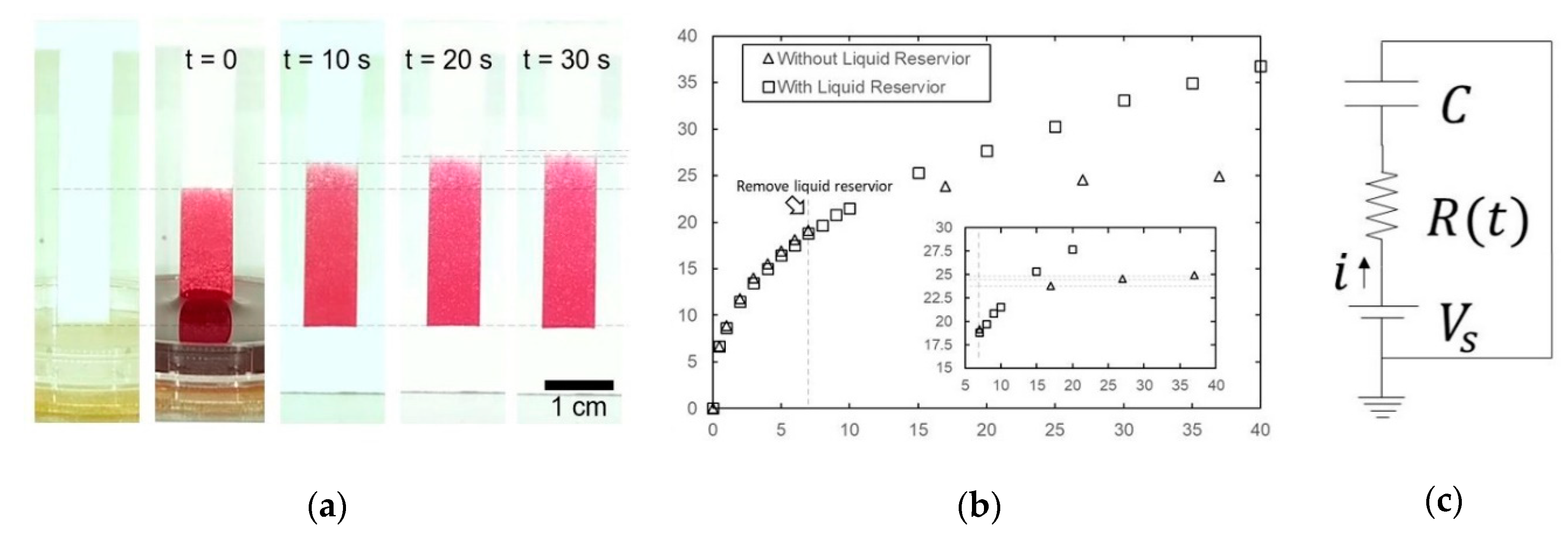
This paper reports an ECA model with a capacitance connected in series with a resistance. In the preliminary experiment, we observed that the paper has the ability to store a liquid in its matrix because the liquid continues to wick after removing the reservoir, Figure 2a,b. Thus, a capacitance for liquid storage should be included in the model similar to the way a capacitor storing charge in an electric circuit. We assume that the fluidic capacitance is a function of properties such as absorption capacity, porosity and surface property of fibrous material. Moreover, the velocity of liquid wicking decreases over time due to the increasing resistance with the advancing liquid front. The circuit of our model for a simple paper strip contains resistance and capacitance which are serially connected under the same applied capillary force, Figure 2c. The model includes the equations describing the current response, resistance and distance over time. Experiments were carried out with paper strips made of different materials and laminating conditions to validate this model.
2. Theoretical Model
In a wicking process, the liquid advances in the paper matrix and at the same time occupies the space in the porous matrix. Figure 2a indicates that the liquid front still advances, when the reservoir was removed. Without a reservoir as the source, the wet paper serves as a capacitor to continue discharging the liquid to the fluidic circuit. This phenomenon leads to the ECA model with a capacitance connected in series with a resistance, Figure 2c. The derivation of the model is performed first in the electric domain. First, Kirchhoff’s voltage law is applied to the analogy circuit. The summation of voltage difference across resistance and capacitance is equal to voltage source (Vs) due to its serial connection described as:
where Vs is the voltage source that is equivalent to the capillary pressure [31], VR is the voltage difference across the resistance R, VC is the voltage difference across the capacitance C. Rearranging Equation (1) into the function of charge Q is described as:
where R(t) is the resistance, Q is the total charge flowing in the circuit, C is the capacitance. Rearranging Equation (2) for integration, the charge equation can be solved:
From the equivalent circuit in Figure 1, the current is equivalent to the mass flow rate. Moreover, the current also has its own relationship with the electron drift speed described as:
where I is the current (A), e is the electron charge (1.6 × 10⁻¹⁹ Coulomb), v is velocity (m/s), Ac is cross-sectional area (m2), n is charge density (1/m3). Given (Coulomb/m3), which is charge with unit volume, this parameter is equivalent to the density of the fluid. Integrating current over time results in the total charge flow:
Therefore, the charge equation from Equation (5) can be formulated as a function of velocity. The distance can be determined as:
where L is the distance function of charge moving in the circuit, C is the capacitance, q is the charge density (C/m3), Ac is cross-sectional area and R(t) is the fluidic resistance function. Given , the unknown coefficients a and b can be determined experimentally with the fitting equation:
Given , the resistance function follows the power law, so the fitting function of the fluidic resistance has the form:
The coefficient a represents the capacitance, which can also be experimentally determined as:
The absorption capacity Cabs (µL) is the ability to store liquid per surface area AS (cm2) of paper strip
According to Figure 1 and the analogy table, the charge moving distance in an electrical circuit is equivalent to the position of liquid front in fluidic network. All electrical parameters were converted into fluidic parameters. Therefore, this model can be used to fit with the experimental data of liquid front distance over time. From Equations (7) and (8), we define coefficients a, b and d to reflect the material properties. These coefficients can be experimentally determined by fitting curve from experimental data. The coefficient a affects the steady value that reflect the saturation of the liquid in the paper. Thus, coefficient a can be linked to liquid absorption capacity of the materials which represents the saturation of paper matrix by Equations (9) and (10). Coefficient b and d related to how fast it can reach the steady value, so it can be interpreted to reflect material characteristics. In addition, the hydraulic capacitance or a compliance of a system in a microfluidic system is the change of effective stored liquid volume per change in pressure. The compliance can be applied under the condition of deformed microchannel. However, in this case, the ability to store the liquid in the paper matrix is different from those observed in a microfluidic system. In this model, the fluidic capacitance is described as a ratio of liquid mass retaining through the paper strip to pressure difference which is capillary pressure defined by the material properties. As a result, the fluidic capacitance is equivalent to capacitance in electrical circuit representing as a ratio of charge accumulation to voltage difference.
3. Materials and Method
3.1. Materials and Instrumentation
The porous materials used in the experiments were cellulose papers (CFSP223000, Merck, New York, NY, USA) and nitrocellulose papers (FF170HP PLUS, Whatman, UK). The laminated polymer film (86624014, Rexel Holdings Australia Pty Ltd., North Ryde, Australia) was two polymer types which are Polyethylene Terephthalate (PET) and Ethylene-vinyl Acetate (EVA). A stock of rose-pink food coloring (082063, Queen Fine Foods Pty Ltd., Alderley, Australia) containing 1.4% dyestuff was diluted in DI water (Milli-Q, Merck, New York, NY, USA) to obtain 0.1% dyestuff in dye solution used in the experiment. Digital weighing machine (ENTRIS124I-1S, Sartorius Lab Instrument, Göttingen, Germany) used to weigh paper in dry and wet conditions. For software, image converter (Free Studio v6.7.1.316, DVDVideoSoft Ltd., London, UK) was used to convert a video file into image sequences. Image processing including fitting the data was performed by numerical computing software (MATLAB R2018b, The MathWorks Inc., Natick, MA, USA).
3.2. Paper Strip Preparation
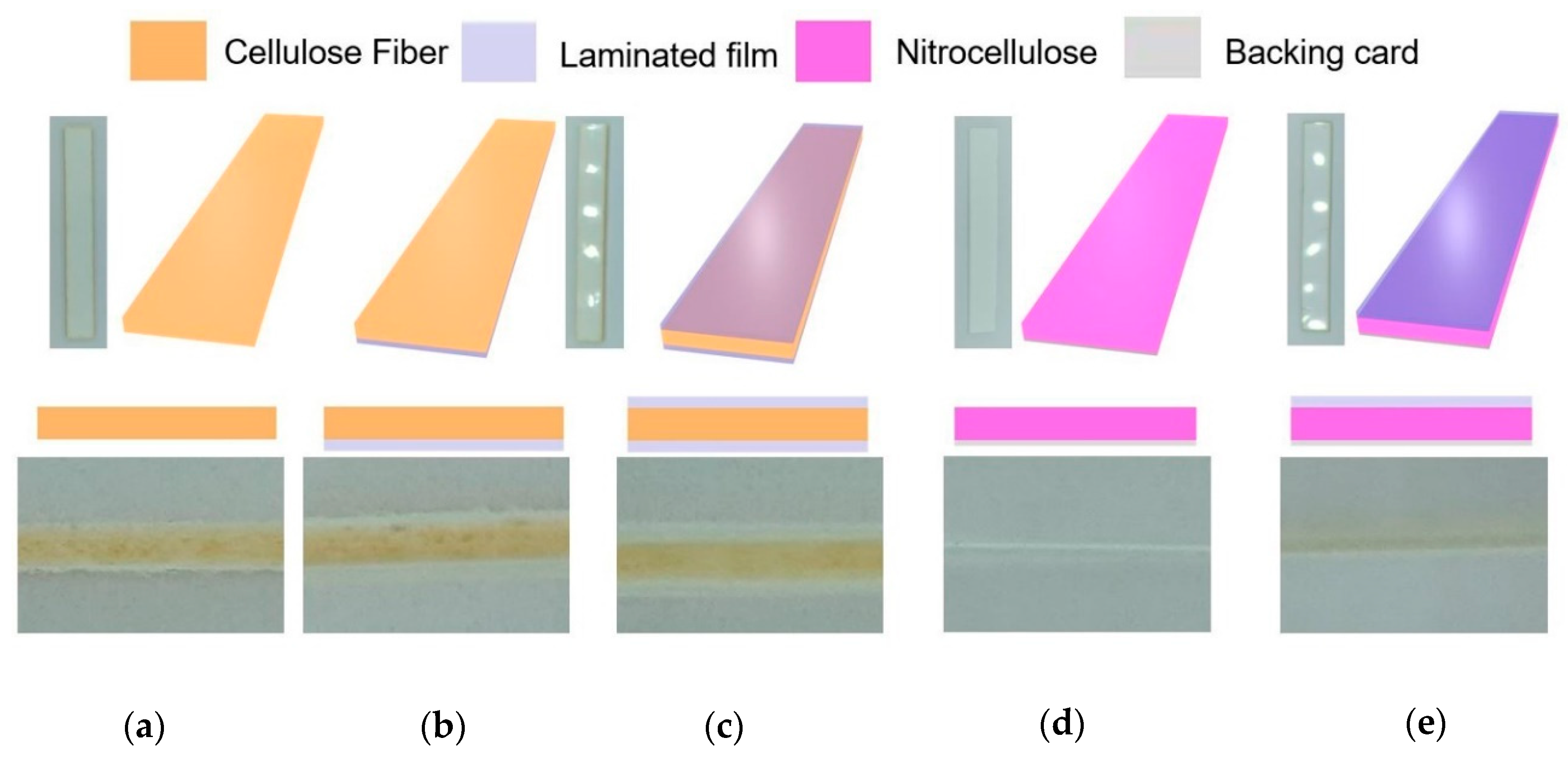
The paper strips were cut using a laser machine (R500 Laser cutter, Rayjet) into widths of 2 mm, 4 mm and 6 mm. A laminated polymer film was applied to the cellulose paper (CFSP) on one side or on both sides. The laminated film was attached to the CFSP using a laminator (JL330T, PFEC) at 130 °C with a feeding speed of 1 cm/s. The laminated CFSP was also cut using the same laser machine. Thus, the CFSP types in our experiments are non-laminated (Figure 3a), one-side laminated (Figure 3b) and both-side laminated (Figure 3c). In the case of nitrocellulose (NC) paper, we only laminated one side because the other side of the off-the-shelf NC (Figure 3d) was already laminated and referred to in this study as laminated NC (Figure 3e). The original off-the-shelf NC paper is referred to as non-laminated NC.
3.3. Experiment Setup and Data Acquisition
Figure 4 shows the schematic and the actual setup for the capillary rise experiment in a paper strip. The paper strip was vertically positioned with a customized acrylic stand. Experiments were carried out for each strip width with a sample number of n = 3. Dye solution served as the fluid wicking up to the paper strip. The camera recorded the image of the paper strip every second for the first ten seconds and every five seconds for the remaining time. Subsequently, the images were processed with MATLAB to measure the position of the liquid front. The images were first imported into MATLAB, and then cropped into the area of interest. Next, the images were adjusted with brightness and contrast to improve the sample-to-background contrast, and then converted into the grayscale format. The processed images were further converted into the binary format for the measurement of the length of the liquid column. The data were then exported to plot the liquid distance over time. The error bars applied to experimental data were two times of standard deviation.
3.4. Fitting Curve Settings
After collecting the data of the liquid column length over time, MATLAB performed curve fitting with the interactive toolbox cftool. We used non-linear least squares with trust-region algorithm to fit the data according to the model of Equation (6). This algorithm is a common mathematical optimization to restrict the fitting result within the range of applied lower and upper boundaries. Finite difference parameters were set for nonlinear equation at the default value at 1 × 10⁻⁸ and 0.1 for minimum and maximum changes, respectively. The maximum iteration and termination tolerance are set at 106 and 10−10 respectively, to make sure that fitting solution converges and fits with the smallest tolerance. Table 1 shows the starting point of iteration, the upper and the lower boundary used for fitting. After fitting with MATLAB, all coefficients in Equation (7) are experimentally determined. The exponential functions have several local solution points. Although curve fitting is performed with many initial boundaries, the result of fitting did not show any significant difference (S.D. is around 0.1% of average values). Therefore, all results were reported as average values. Table 2 lists the values used in the calculation. For Washburn model, the experimental data of the liquid front were fitted as a square root function of time:
where p is a fitting coefficient for Washburn model. Each experiment data set was fitted, and coefficient p will be identified.
3.5. Direct Measurement for Liquid Absorption Capacity
All paper strips were cut with the laser machine into of 1 × 1 cm, 1.5 × 1.5 cm and 2 × 2 cm pieces. Consequently, the paper pieces were weighed in dry and wet conditions. For the wet conditions, the paper pieces were immersed in dye solution for 2–3 min to make sure that paper pieces were saturated, Figure 5. The liquid absorption capacity was determined by the equation described as:
where and are the paper piece mass in wet and dry conditions respectively. The mass difference between both conditions determines the amount of fluid retained in the paper strip.
4. Result and Discussion
4.1. Fitting for Cellulose Fiber Paper
According to the power law, coefficient d determines the slope of exponential curve to reach a steady value. Therefore, coefficient d represents the wicking speed which depends on the material properties. We began fitting the model with experimental data of non-laminated CFSPs. The fitting approach is performed with data from all strip sizes to obtain coefficients a, b and d from the experiment data. Table 3 and Table 4 shows the average fitting coefficients for non-laminated CFSP. From these results, the coefficient d for the cellulose paper was selected as 0.4. All CFSP cases will use this value for further analysis. The average coefficient a and b are 1.14 × 10⁸ and 7.53 × 10⁻⁸, respectively. The fitting procedure was performed for the case of non-laminated cellulose paper. One-side laminated CFSP was subsequently investigated. The average coefficient a and b for one-side laminated CFSP are 1.12 × 10⁸ and 6.31 × 10⁻⁸, respectively. Finally, two-side laminated CFSP was investigated. The two-side lamination helps to improve the strength of the test strip and prevents evaporation. The average coefficients a and b for two-side laminated CFSP are 1.12 × 10⁸ and 6.51 × 10⁻⁸, respectively. Thus, our model agrees well with experimental data of all conditions: non-laminated, one-side and two-side laminated CFSP, Figure 6. The characteristic of wicking speed and material is represented by the coefficient d in the model, which is 0.4. It is dictated by the power law resulting in the steep curve in the early period. As a result, this model fits experimental data better than the Washburn model.
4.2. Fitting for Nitrocellulose Paper
The fitting procedure was performed to determine all coefficients for non-laminated NC paper, Table 5 and Table 6. The coefficient d was selected as 0.5 for NC paper and represents its material characteristics. Using coefficient d as 0.5, the average coefficients a and b were determined as 1.06 × 10⁸ and 2.95 × 10⁻⁸, respectively. For laminated NC, the average coefficient a and b are 1.05 × 10⁸ and 2.68 × 10⁻⁸, respectively. As a result, the model in both conditions is in good agreement with both experimental conditions: non-laminated NC and laminated NC as shown in Figure 7. As the coefficient d is 0.5, this model provides a similar relationship between liquid front distance and the square root of time as Washburn model. As a result, both CFSP and NC materials agree well with conventional Washburn model.
4.3. Absorption Capacity
The absorption capacity from direct measurement is shown in Figure 8. For CFSP cases (Figure 8a), the absorption capacity of two-side laminated CFSP is 65.2 µL/cm2 which is lower than other cases, which are one-side laminated (76.7 µL/cm2) and non-laminated (79.3 µL/cm2). For NC cases (Figure 8b), laminated NC (6.42 µL/cm2) also provide lower absorption capacity than non-laminated NC (10.1 µL/cm2). As a result, laminated film was melted and permeated into paper matrix resulting in reduced space in the paper matrix. Furthermore, our model with fitting coefficients can also predict the absorption capacity. We obtained the absorption capacity from the model through coefficient a and Equations (9) and (10). The absorption capacity estimated with the model has the same order of magnitude as those from direct weighting and from the literature, Table 7. The Cabs of non-laminated CFSP and NC papers provides 5.77% and 18.9% error respectively compared to the absorption capacity from direct weighting experiment. However, the absorption capacity of both CFSP and NC cases from direct weighting experiment are not statistically different from the model under p value of <0.01. The discrepancy may come from the environment factors such as temperature or humidity, which affect the ability of the paper to store liquid. Thus, we conclude that our model can predict the absorption capacity and can be further used for predicting capillary pressure in each material as discussed later in Section 4.5.
4.4. Fluidic Resistance Function
The fluidic resistance can be estimated with Equation (8) and depicted in Figure 9 and Figure 10 for CFSP and NC cases, respectively. The resistance is a function of time which increases according to the power law and the exponential terms. The fluidic resistance is mainly defined by the fitting coefficient b which dictates the slope and is similar for the same material. The larger the cross-sectional area, the smaller is the fluidic resistance. The fluidic resistance of the laminated cases has a larger value than non-laminated cases, because the capacitance decreases according to Equation (8). The data in Figure 8 showed that the absorption capacity measured from direct weighting decreases in the case of laminated conditions as the laminated film was melted and permeated into the paper matrix. Moreover, the hydrophobicity may also affect the fluidic resistance. Some studies reported that capillary force exerting on fluid in wax-boundary paper is in the opposite direction of fluid flow [17]. As a result, wicking speed depends on strip width due to the hydrophobic boundary [17,32]. Nevertheless, our experiments showed that even though the fluidic resistance increases with decreasing strip width, the wicking speed of all widths is almost the same, Figure 6 and Figure 7 [22,30]. The laminated film has hydrophilic surface properties (contact angle of 43°), so the capillary force at the laminated surface will not act against the wicking speed direction. Thus, the hydrophilicity of the laminated film maintained wicking speed in paper strips with different widths.
4.5. Capillary Pressure
One of the important parameters of the ECA model is the capillary pressure represented by a constant voltage source. Defining an accurate capillary pressure in the paper strip is still challenging, because it requires complex and specific setup [14]. According to Equations (9) and (10), the capillary pressure can be experimentally determined by our model, Table 8. The evaluated capillary pressure has the same order of magnitude as those reported in the literature [30]. For example, the capillary pressure of non-laminated CFSP and nitrocellulose membrane are 2586 Pa and 2345 Pa, which are 13.8% and 22.8% difference from the literature and approximation (Appendix A) respectively. According to Equations (9) and (10), the capillary pressure depends on coefficient a, fluid density, paper strip length, liquid absorption capacity and paper strip thickness. These parameters can be affected by the lamination procedures. For the laminated cases, the relative difference of capillary pressure between the model and the literature probably caused by the slightly different cross-sectional areas due to the lamination and hydrophilicity of the lamination. Therefore, the capillary pressure can be estimated by fitting experimental data with this model.
5. Conclusions
The ECA model can be used to describe flow in paper strips and has been reported previously. However, previous models did not include the properties and the porous nature of paper-based materials. In this paper, we proposed a model that accounts for the absorption capacity through the capacitance of the fluidic circuit. All data were obtained from the capillary rise experiment of a straight vertical paper strips. The data were processed and fitted with the model to determine all coefficients. The ECA model agrees well with experimental data. Furthermore, each coefficient is interpreted and compared with values reported elsewhere by converting the electric parameters to fluidic parameters. Our model can explain the dependence of fluidic resistance on the material characteristics. The smaller is the paper strip width, the larger is the fluidic resistance. The laminated cases also provided a larger resistance because lamination may reduce the thickness of the paper strip. It is worth noting that the ECA model reported here also agrees well with the traditional Washburn model which is well-known for describing fluid flow in porous media. However, our ECA model further allows for the determination of material properties. In addition to the fluidic resistance, the model can be used to predict the capillary pressure using the fitting coefficients and the absorption capacity determined by the model. The estimated capillary pressure agrees well with values reported in the literature.
Author Contributions
Conceptualization, methodology, validation, data curation, writing-original draft preparation, S.K., M.J.A.S., N.-T.N.; writing-review and editing, supervision, M.J.A.S., N.-T.N. All authors have read and agreed to the published version of the manuscript.
Funding
This research was funded by Australian Research Council, grant number DP180100055. S.K. was funded by higher degree research scholarships GUIPRS and GUPRS Scholarships of the Griffith University.
Conflicts of Interest
The authors declare no conflict of interest.
Appendix A
The label of the paper product indicates the time in second of the liquid flow in a 4-cm paper strip. For instance, FF080HP means liquid flows in 4-cm long nitrocellulose membrane in 80 s, or FF170HP takes 170 s for liquid to flow in 4-cm long nitrocellulose membrane. The membrane characteristics such as pore size or porosity determine the flow in membrane. Capillary pressure is also affected because it is defined by the membrane properties. From the literature, capillary pressure of FF080HP is equal to 13,000 Pa as shown in Table 1. However, in this experiment, FF170HP is used. Moreover, as the time used for liquid to flow between these two membranes is different. The capillary pressure of FF170HP is approximately estimated with the dynamic pressure
where P is the dynamic pressure, ρ is fluid density and υ is velocity. The pressure is proportional to the square of the velocity. As known from the product label, the average speed can be approximated by total distance fluid flow which is 4 cm divided by flowing time taken by each membrane. The pressure of FF170HP is 2879 Pa, which is reasonable because FF170HP allows liquid to wick slower than FF080HP originated from smaller capillary pressure. This value is used for this experiment to determine all coefficients in the proposed model.
References
- Eaidkong, T.; Mungkarndee, R.; Phollookin, C.; Tumcharern, G.; Sukwattanasinitt, M.; Wacharasindhu, S. Polydiacetylene paper-based colorimetric sensor array for vapor phase detection and identification of volatile organic compounds. J. Mater. Chem. 2012, 22, 5970–5977. [Google Scholar] [CrossRef]
- Hossain, S.M.Z.; Brennan, J.D. β-Galactosidase-Based Colorimetric Paper Sensor for Determination of Heavy Metals. Anal. Chem. 2011, 83, 8772–8778. [Google Scholar] [CrossRef]
- Jokerst, J.C.; Adkins, J.A.; Bisha, B.; Mentele, M.M.; Goodridge, L.D.; Henry, C.S. Development of a Paper-Based Analytical Device for Colorimetric Detection of Select Foodborne Pathogens. Anal. Chem. 2012, 84, 2900–2907. [Google Scholar] [CrossRef]
- Vella, S.J.; Beattie, P.; Cademartiri, R.; Laromaine, A.; Martinez, A.W.; Phillips, S.T.; Mirica, K.A.; Whitesides, G.M. Measuring Markers of Liver Function Using a Micropatterned Paper Device Designed for Blood from a Fingerstick. Anal. Chem. 2012, 84, 2883–2891. [Google Scholar] [CrossRef] [Green Version]
- Sajid, M.; Kawde, A.-N.; Daud, M. Designs, formats and applications of lateral flow assay: A literature review. J. Saudi Chem. Soc. 2015, 19, 689–705. [Google Scholar] [CrossRef] [Green Version]
- Wong, R.; Tse, H. Lateral Flow Immunoassay, 1st ed.; Humana Press: Totowa, NJ, USA, 2009. [Google Scholar] [CrossRef]
- Kasetsirikul, S.; Shiddiky, M.J.A.; Nguyen, N.-T. Challenges and perspectives in the development of paper-based lateral flow assays. Microfluid Nanofluidics 2020, 24, 17. [Google Scholar] [CrossRef]
- Dungchai, W.; Chailapakul, O.; Henry, C.S. Use of multiple colorimetric indicators for paper-based microfluidic devices. Anal. Chim. Acta 2010, 674, 227–233. [Google Scholar] [CrossRef]
- Avoundjian, A.; Jalali-Heravi, M.; Gomez, F.A. Use of chemometrics to optimize a glucose assay on a paper microfluidic platform. Anal. Bioanal. Chem. 2017, 409, 2697–2703. [Google Scholar] [CrossRef]
- Hamedpour, V.; Oliveri, P.; Leardi, R.; Citterio, D. Chemometric challenges in development of paper-based analytical devices: Optimization and image processing. Anal. Chim. Acta 2020, 1101, 1–8. [Google Scholar] [CrossRef]
- Jalali-Heravi, M.; Arrastia, M.; Gomez, F.A. How Can Chemometrics Improve Microfluidic Research? Anal. Chem. 2015, 87, 3544–3555. [Google Scholar] [CrossRef]
- Scampicchio, M.; Mannino, S.; Zima, J.; Wang, J. Chemometrics on Microchips: Towards the Classification of Wines. Electroanalysis 2005, 17, 1215–1221. [Google Scholar] [CrossRef]
- Shariati-Rad, M.; Irandoust, M.; Mohammadi, S. Multivariate analysis of digital images of a paper sensor by partial least squares for determination of nitrite. Chemom. Intell. Lab. Syst. 2016, 158, 48–53. [Google Scholar] [CrossRef]
- Liu, Z.; He, X.; Han, J.; Zhang, X.; Li, F.; Li, A.; Qu, Z.; Xu, F. Liquid wicking behavior in paper-like materials: Mathematical models and their emerging biomedical applications. Microfluid Nanofluidics 2018, 22, 132. [Google Scholar] [CrossRef]
- Liu, Z.; Hu, J.; Zhao, Y.; Qu, Z.; Xu, F. Experimental and numerical studies on liquid wicking into filter papers for paper-based diagnostics. Appl. Therm. Eng. 2015, 88, 280–287. [Google Scholar] [CrossRef]
- Jahanshahi-Anbuhi, S.; Chavan, P.; Sicard, C.; Leung, V.; Hossain, S.M.Z.; Pelton, R.; Brennan, J.D.; Filipe, C.D.M. Creating fast flow channels in paper fluidic devices to control timing of sequential reactions. Lab. A Chip 2012, 12, 5079–5085. [Google Scholar] [CrossRef]
- Hong, S.; Kim, W. Dynamics of water imbibition through paper channels with wax boundaries. Microfluid Nanofluidics 2015, 19, 845–853. [Google Scholar] [CrossRef]
- Lioumbas, J.S.; Zamanis, A.; Karapantsios, T.D. Towards a wicking rapid test for rejection assessment of reused fried oils: Results and analysis for extra virgin olive oil. J. Food Eng. 2013, 119, 260–270. [Google Scholar] [CrossRef]
- Ponomarenko, A.; QuÉRÉ, D.; Clanet, C. A universal law for capillary rise in corners. J. Fluid Mech. 2011, 666, 146–154. [Google Scholar] [CrossRef] [Green Version]
- Washburn, E.W. The Dynamics of Capillary Flow. Phys. Rev. 1921, 17, 273–283. [Google Scholar] [CrossRef]
- Elizalde, E.; Urteaga, R.; Berli, C.L.A. Rational design of capillary-driven flows for paper-based microfluidics. Lab. A Chip 2015, 15, 2173–2180. [Google Scholar] [CrossRef]
- Fu, E.; Ramsey, S.A.; Kauffman, P.; Lutz, B.; Yager, P. Transport in two-dimensional paper networks. Microfluid Nanofluidics 2011, 10, 29–35. [Google Scholar] [CrossRef] [Green Version]
- Parolo, C.; Medina-Sánchez, M.; de la Escosura-Muñiz, A.; Merkoçi, A. Simple paper architecture modifications lead to enhanced sensitivity in nanoparticle based lateral flow immunoassays. Lab. A Chip 2013, 13, 386–390. [Google Scholar] [CrossRef] [Green Version]
- Richards, L.A. CAPILLARY CONDUCTION OF LIQUIDS THROUGH POROUS MEDIUMS. Physics 1931, 1, 318–333. [Google Scholar] [CrossRef]
- Whitaker, S. Flow in porous media I: A theoretical derivation of Darcy’s law. Transp. Porous Media 1986, 1, 3–25. [Google Scholar] [CrossRef]
- Ge, W.-K.; Lu, G.; Xu, X.; Wang, X.-D. Droplet spreading and permeating on the hybrid-wettability porous substrates: A lattice Boltzmann method study. Open Phys. 2016, 14, 483. [Google Scholar]
- Hyväluoma, J.; Raiskinmäki, P.; Jäsberg, A.; Koponen, A.; Kataja, M.; Timonen, J. Simulation of liquid penetration in paper. Phys. Rev. E 2006, 73, 036705. [Google Scholar] [CrossRef]
- Sadeghi, M.A.; Aghighi, M.; Barralet, J.; Gostick, J.T. Pore network modeling of reaction-diffusion in hierarchical porous particles: The effects of microstructure. Chem. Eng. J. 2017, 330, 1002–1011. [Google Scholar] [CrossRef] [Green Version]
- Tang, R.; Yang, H.; Gong, Y.; Liu, Z.; Li, X.; Wen, T.; Qu, Z.; Zhang, S.; Mei, Q.; Xu, F. Improved Analytical Sensitivity of Lateral Flow Assay using Sponge for HBV Nucleic Acid Detection. Sci. Rep. 2017, 7, 1360. [Google Scholar] [CrossRef] [Green Version]
- Toley, B.J.; McKenzie, B.; Liang, T.; Buser, J.R.; Yager, P.; Fu, E. Tunable-delay shunts for paper microfluidic devices. Anal. Chem. 2013, 85, 11545–11552. [Google Scholar] [CrossRef] [Green Version]
- Fries, N. Capillary Transport Processes in Porous Materials–Experiment and Model. Ph.D. Thesis, Universität Bremen, Göttingen, Germany, 2010. [Google Scholar]
- Li, X.; Zwanenburg, P.; Liu, X. Magnetic timing valves for fluid control in paper-based microfluidics. Lab. A Chip 2013, 13, 2609–2614. [Google Scholar] [CrossRef]
Figure 1.
The equivalent circuit comparison between electrical circuit and fluidic circuit and parameter equivalence table including unit analysis.
Figure 1.
The equivalent circuit comparison between electrical circuit and fluidic circuit and parameter equivalence table including unit analysis.

Figure 2.
The ability to store liquid in paper matrix was observed (a) the sequential observed photos depicted the progress of liquid front after removing the liquid reservoir (b) the comparison of experimental data between with liquid reservoir and without liquid reservoir. (c) schematic diagram of an equivalent circuit for wicking in a paper strip with liquid reservoir.

Figure 3.
Paper types used in the experiment: (a) non-laminated CFSP, (b) one-side laminated CFSP, (c) both-side laminated CFSP, (d) nitrocellulose (NC) membrane, (e) laminated nitrocellulose membrane.
Figure 3.
Paper types used in the experiment: (a) non-laminated CFSP, (b) one-side laminated CFSP, (c) both-side laminated CFSP, (d) nitrocellulose (NC) membrane, (e) laminated nitrocellulose membrane.

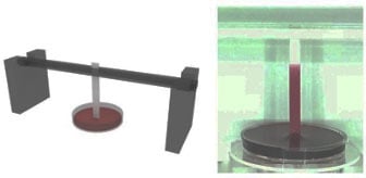
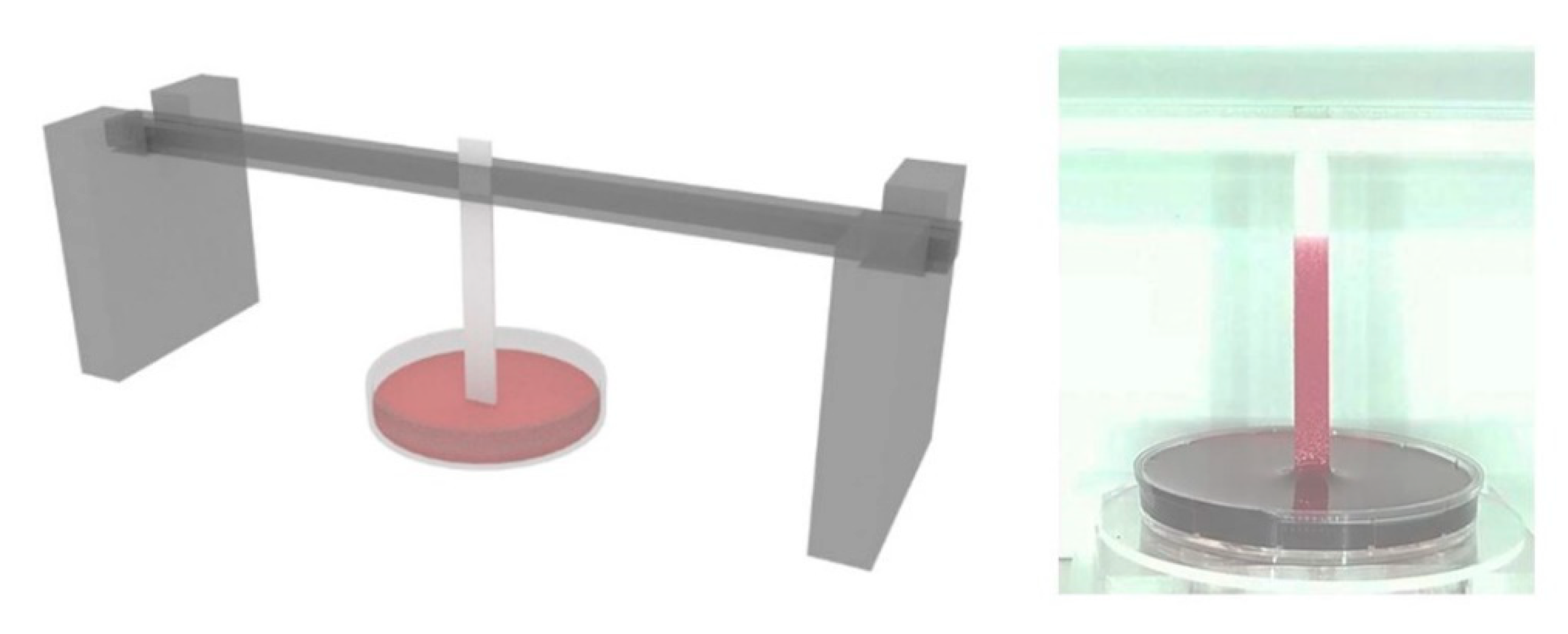
Figure 4.
Schematic diagram of experiment setup.

Figure 5.
The experiment diagram of direct measurement of absorption capacity.

Figure 6.
Comparison between our model and experiment data (a) non-laminated CFSP, (b) one-side laminated CFSP and (c) two-side laminated CFSP.
Figure 6.
Comparison between our model and experiment data (a) non-laminated CFSP, (b) one-side laminated CFSP and (c) two-side laminated CFSP.

Figure 7.
Comparison between our model and experiment data for (a) non-laminated NC paper and (b) laminated NC paper.
Figure 7.
Comparison between our model and experiment data for (a) non-laminated NC paper and (b) laminated NC paper.

Figure 8.
Comparison between our model and experiment data for (a) non-laminated NC paper and (b) laminated NC paper. Sample n = 3 for independent experiments.
Figure 8.
Comparison between our model and experiment data for (a) non-laminated NC paper and (b) laminated NC paper. Sample n = 3 for independent experiments.

Figure 9.
The fluidic resistance over time: (a) Non-laminated CFSP with various widths of paper strips (b) for one-side laminated CFSP; (c) Two-side laminated CFSP; (d) Various laminated conditions under the same width 4 mm of paper strips.
Figure 9.
The fluidic resistance over time: (a) Non-laminated CFSP with various widths of paper strips (b) for one-side laminated CFSP; (c) Two-side laminated CFSP; (d) Various laminated conditions under the same width 4 mm of paper strips.

Figure 10.
The fluidic resistance over time: (a) Non-laminated NC with various widths of paper strips (b) Laminated NC (c) Various laminated conditions under the same width of paper strips.
Figure 10.
The fluidic resistance over time: (a) Non-laminated NC with various widths of paper strips (b) Laminated NC (c) Various laminated conditions under the same width of paper strips.


Table 1.
List of initial points, upper and lower boundary.
| Coefficient | Starting Points | Lower Boundary | Upper Boundary |
|---|---|---|---|
| a | 1 × 10⁸–1 × 10⁹ | 1 × 10⁸ | 1 × 10⁹ |
| b | 0.001–0.999 | 0 | 1 |
| d | 0.001–0.999 | 0 | 1 |
Table 2.
List of constant values used in the calculation.
| Parameter | Value |
|---|---|
| Vs-Pressure-Capillary pressure in CFSP | 3000 Pa [30] |
| Vs-Pressure-Capillary pressure in Nitrocellulose (FF80HP) | 13,000 Pa [30] |
| Vs-Pressure-Capillary pressure in Nitrocellulose (FF170HP) | 2879 Pa * |
| Adsorption capacity in CFSP | 79.29 µL/cm2 [30] |
| Adsorption capacity in Nitrocellulose (FF170HP) | 10.06 µL/cm2 [30] |
| Viscosity | 8.94 × 10⁻⁴ Pa.s |
| Density | 1000 kg/m3 |
* Capillary pressure of FF170HP is determined as shown in Appendix A.
Table 3.
Fitting coefficients of non-laminated CFSP paper by our model.
| Non-Laminated CFSP Size | a | b | d |
|---|---|---|---|
| 2 mm | 1.02 × 10⁸ | 8.14 × 10⁻⁸ | 0.40 |
| 4 mm | 1.03 × 10⁸ | 8.63 × 10⁻⁸ | 0.39 |
| 6 mm | 1.02 × 10⁸ | 8.69 × 10⁻⁸ | 0.39 |
Table 4.
Fitting coefficient p of Washburn relation of CFSP paper.
| Materials | Coefficient p for Washburn Relation | |||
|---|---|---|---|---|
| Width 2 mm | Width 4 mm | Width 6 mm | Average | |
| Non-laminated CFSP | 6.05 | 6.14 | 6.25 | 6.15 |
| One-side laminated CFSP | 4.47 | 4.86 | 4.96 | 4.76 |
| Two-side laminated CFSP | 5.08 | 4.93 | 5.08 | 5.03 |
Table 5.
Fitting coefficients of non-laminated NC paper by our model.
| Non-Laminated NC Size | a | b | d |
|---|---|---|---|
| 2 mm | 1.02 × 10⁸ | 3.03 × 10⁻⁸ | 0.50 |
| 4 mm | 1.02 × 10⁸ | 3.41 × 10⁻⁸ | 0.48 |
| 6 mm | 1.01 × 10⁸ | 3.00 × 10⁻⁸ | 0.52 |
Table 6.
Fitting coefficient p of Washburn relation of NC paper.
| Materials | Coefficient p for Washburn Relation | |||
|---|---|---|---|---|
| Width 2 mm | Width 4 mm | Width 6 mm | Average | |
| Nitrocellulose membrane | 3.08 | 3.18 | 3.12 | 3.12 |
| Laminated nitrocellulose membrane | 2.75 | 2.94 | 2.80 | 2.83 |
Table 7.
Absorption capacity result from the model and direct weighting experiment comparing to literature.
Table 7.
Absorption capacity result from the model and direct weighting experiment comparing to literature.
| Non-Laminated CFSP (µL/cm2) | Nitrocellulose Membrane (µL/cm2) | |
|---|---|---|
| Absorption capacity from the model | 75.0 | 8.14 |
| Absorption capacity from the direct weighting experiment | 79.3 | 10.07 |
| Absorption capacity from literature | 83 [30] | 10 [30] |
Table 8.
The capillary pressure estimated by our model.
| Materials | Absorption Capacity (µL/cm2) | Coefficient a | Capillary Pressure (Pa) |
|---|---|---|---|
| Non-laminated CFSP | 79.3 ± 1.60 | 1.14 × 10⁸ | 2586 |
| One-side laminated CFSP | 76.7 ± 3.49 | 1.12 × 10⁸ | 2881 |
| Two-side laminated CFSP | 65.2 ± 2.93 | 1.12 × 10⁸ | 3522 |
| Nitrocellulose membrane | 10.1 ± 1.85 | 1.06 × 10⁸ | 2345 |
| Laminated nitrocellulose membrane | 6.42 ± 0.25 | 1.06 × 10⁸ | 3636 |
© 2020 by the authors. Licensee MDPI, Basel, Switzerland. This article is an open access article distributed under the terms and conditions of the Creative Commons Attribution (CC BY) license (http://creativecommons.org/licenses/by/4.0/).
Share and Cite
MDPI and ACS Style
Kasetsirikul, S.; Shiddiky, M.J.A.; Nguyen, N.-T. Wicking in Paper Strips under Consideration of Liquid Absorption Capacity. Chemosensors 2020, 8, 65. https://0-doi-org.brum.beds.ac.uk/10.3390/chemosensors8030065
AMA Style
Kasetsirikul S, Shiddiky MJA, Nguyen N-T. Wicking in Paper Strips under Consideration of Liquid Absorption Capacity. Chemosensors. 2020; 8(3):65. https://0-doi-org.brum.beds.ac.uk/10.3390/chemosensors8030065
Chicago/Turabian StyleKasetsirikul, Surasak, Muhammad J. A. Shiddiky, and Nam-Trung Nguyen. 2020. "Wicking in Paper Strips under Consideration of Liquid Absorption Capacity" Chemosensors 8, no. 3: 65. https://0-doi-org.brum.beds.ac.uk/10.3390/chemosensors8030065
Note that from the first issue of 2016, this journal uses article numbers instead of page numbers. See further details here.