
Drift Compensation on Massive Online Electronic-Nose Responses
by
 ,
,
Jianhua Cao
1,2, 
Tao Liu
1,2,*,
Jianjun Chen
1,2,*,
Tao Yang
1,2,
Xiuxiu Zhu
1,2 and
Hongjin Wang
1,2 1
School of Microelectronics and Communication Engineering, Chongqing University, Chongqing 400044, China
2
Chongqing Key Laboratory of Bio-Perception & Intelligent Information Processing, Chongqing University, Chongqing 400044, China
*
Authors to whom correspondence should be addressed.
Chemosensors 2021, 9(4), 78; https://0-doi-org.brum.beds.ac.uk/10.3390/chemosensors9040078
Submission received: 3 March 2021
/
Revised: 7 April 2021
/
Accepted: 8 April 2021
/
Published: 11 April 2021
(This article belongs to the Collection State-of-the-Art in Chemical Sensors Modelling and Theoretical Statements)
Abstract
:Gas sensor drift is an important issue of electronic nose (E-nose) systems. This study follows this concern under the condition that requires an instant drift compensation with massive online E-nose responses. Recently, an active learning paradigm has been introduced to such condition. However, it does not consider the “noisy label” problem caused by the unreliability of its labeling process in real applications. Thus, we have proposed a class-label appraisal methodology and associated active learning framework to assess and correct the noisy labels. To evaluate the performance of the proposed methodologies, we used the datasets from two E-nose systems. The experimental results show that the proposed methodology helps the E-noses achieve higher accuracy with lower computation than the reference methods do. Finally, we can conclude that the proposed class-label appraisal mechanism is an effective means of enhancing the robustness of active learning-based E-nose drift compensation.
1. Introduction
An electronic nose (E-nose) is a kind of odor-sensing device containing a gas sensor array and proper recognition algorithms [1,2]. The gas sensor is a fundamental part of an E-nose, and the issue of gas sensor drift heavily impedes the performance stability of E-noses. To address this problem, users are often demanded to perform a series of drift calibration experiments to retrain the recognition algorithms, which leads to compulsory pauses during routine works. It is apparently unsuitable for online tasks requiring continuous gas sensing, such as toxic gas alarm [3,4], air pollution monitoring [5,6], gas source tracking [7,8], and intensity measurement of gas mixtures [9,10,11].
Regarding studies on E-noses, drift compensation is still appealing to researchers focusing on two points: signal preprocessing approach [12,13,14,15,16,17,18] and machine learning model [19,20,21,22,23,24,25]. For signal preprocessing, classical signal decomposition approaches (e.g., principal component analysis (PCA), orthogonal signal correction, independent component analysis, and wavelet analysis) have been used to filter out driftlike signals. On the other hand, machine learning methods have tried to obtain proper data space projection for drift data via a multiobjective model and associated solution process. Generally, both types more or less require a number of drift calibration samples with class labels provided from extra drift calibration experiments or algorithmic inferences. However, it seems to be unrealistic in online odor monitoring for extensive and successive E-nose responses, and weak in robustness due to uncertain class labels.
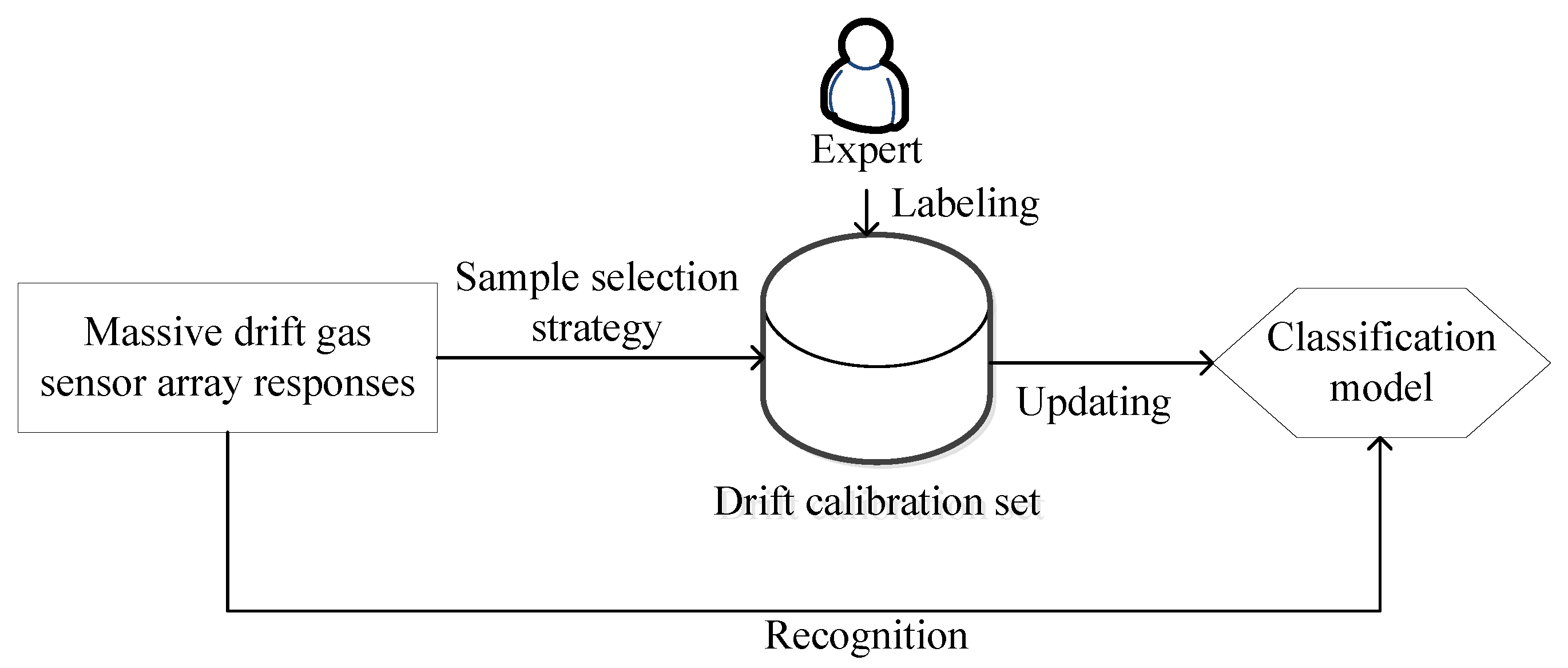
To gain valuable drift calibration samples and associated class labels without any time-consuming experiments, an active learning (AL) paradigm has been introduced in the latest academic publication [26]. As Figure 1 shows, AL allows drift compensation (classification model updating) without any time pauses during odor recognition. It selects the most informative drift calibration samples in a small number from incoming massive drift gas sensor array responses. Meanwhile, selected samples are labeled by a human expert (odor discriminator) immediately. Then, both selected samples and provided labels are added into a drift calibration set to update classification models of E-noses. However, the AL paradigm highly trusts the expert’s annotation, which may deteriorate the recognition performance when the expert is affected by a series of considerable factors (e.g., inattentive errors, lack of experience, and environmental disturbance). Here, we name this matter as “noisy label” problem.
In this study, we aim to detect the suspect class labels of drift calibration samples and ask the expert to relabel. The proposed methodology, named mislabel probability estimation method based on a Gaussian mixture model (MPEGMM), performs class-label appraisal by indicating the potential mislabel probability of each drift calibration sample. In the proposed methodology, under the assumption that drift responses vary slowly with time, the mislabel probability is calculated according to the label disagreement degree between a Gaussian model and the human expert. Then, the labeled samples with high mislabel probability should be relabeled and achieve correct class labels from the human expert. Finally, the renewed drift calibration set can be used for classification model updating. Two E-nose drift datasets, one a public benchmark and the other collected from an E-nose we designed, were generated and collected for the compensation performance assessment. The experimental results show that the proposed method can satisfactorily identify the mislabeled drift calibration samples on presented data. In the meantime, the recognition results after the relabeling of the proposed methodology reach higher accuracy than those of the reference methods. Finally, the novelty behind MPEGMM is reflected threefold: (1) supporting online drift calibration under suspect class labels, (2) adopting a Gaussian mixture model to endure slow data distortion caused by gas sensor drift, and (3) relabeling budget to be adaptively determined to avoid unnecessary computation.
The rest of the paper is organized as follows: Section 2 describes the related works on noisy-label detection of AL. In Section 3, we illustrate the proposed method and associated steps. Then, the experimental results and discussions are presented in Section 4. Finally, Section 5 concludes this paper.
2. Related Works
The class label queried from an expert is conventionally assumed as an oracle in AL methods. That is to say, common AL methods do not contain an appraisal mechanism for obtained class labels. Thus, typical active learning methods are incapable of resisting the negative effect caused by incorrect class labels. These incorrect class labels are seen as noisy labels in the drift calibration set for E-nose drift compensation.
As far as we know, the “noisy label” problem of AL can be treated by class-label appraisal methods in two manners. The first manner is to generate a reliable label from multiple experts [27,28,29]. Although this manner can quickly provide the denoising label, the cost of using multiple experts may become a serious concern in practical usage. Thus, the second strategy depends on a single expert instead of multiple experts to save labor costs: a mislabeled instance would be decided based on the label information of tested instances [30]. Considering that a k-NN classifier is sensitive to label noise, Wilson et al. adopted 3-NN to remove the instance whose label was different from the classifier output [31]. Further, Bouguelia et al. measured the disagreement level of classifier outputs from one expert, judging the incorrect labels on the likelihood [32,33]. Additionally, a novel bidirectional AL method picked up the mislabeled sample with minimum expected entropy under different label assumptions [34]. However, the above solutions were designed for data in a unique distribution, which was unsuitable for drifted data with gradual distribution movement. Thus, it is necessary to propose a one-expert methodology for a noisy-label problem on slow-varying data. As shown in Table 1, we compare our proposed MPEGMM with the other methods mentioned in three aspects (accuracy, adaptation, cost). It can be seen that our method not only obtains higher accuracy and adaptation but also consumes less cost.
3. Methodology
3.1. Improved Active Learning Framework for E-Nose Drift Compensation
AL attempts to select a limited number drift calibration samples from historical instances for classifier updating. The common steps of AL-based drift calibration are summarized in Algorithm 1.
| Algorithm 1. Traditional AL-based drift calibration method. |
| Input: Drift calibration set L, unlabeled historical sample set U. |
| N: number of selected samples (budget). |
| F(x): an instance selection strategy. |
| Output: updated classifier h. |
| 1: Initialize: copy set L’ = L, current selected-sample set S = ∅. |
| 2: for n = 1, 2, …, N do |
| 3: Select the most valuable instance x* by F(x). |
| 4: Label x* as y by a single expert. |
| 5: Update L’: S ← S ∪ {x*,y}, L’ ← L ∪ S, U ← U/{x*}. |
| 6: Update current classifier h by L’. |
| 7: end for |
| 8: Return classifier h. |
Especially, we adopted “uncertainty sampling (US)” as the sample selection strategy F(x) in following sections due to its popularity. Among various measuring metrics of US, we chose “posterior probability margin” (marginu) [35] to represent the uncertainty of an instance xu as follows:
where represents the posterior probability computed by a single classifier h, and and represent the categories predicted by the maximum and second maximum posterior probability, respectively. Therefore, smaller marginu means greater uncertainty. As Formula (2) describes, the selected sample x* should be the one with the minimum marginu in the unlabeled historical sample set U.
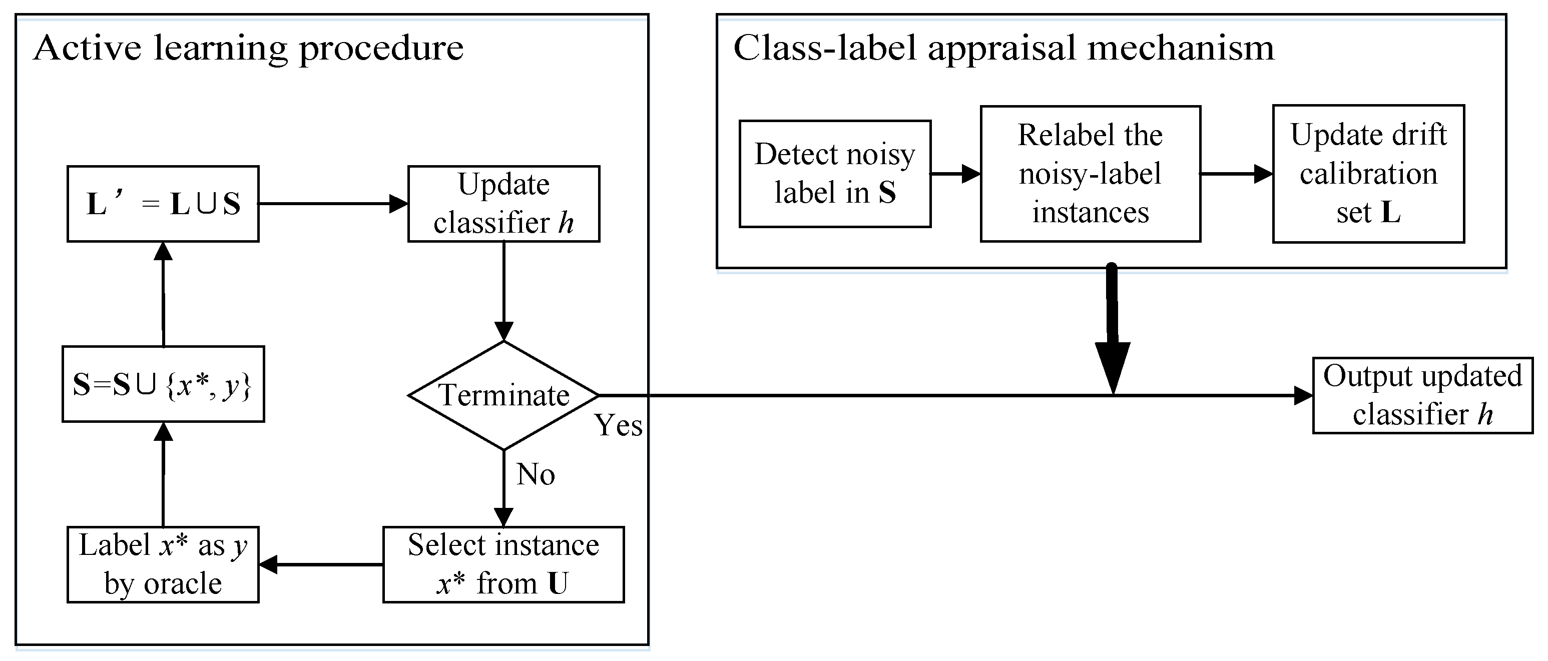
Considering that the expert might provide noisy (error) labels, it is necessary to detect the mislabeled instances and deliver them to the expert for relabeling. Hence, we modified the traditional framework by injecting a “class-label appraisal” mechanism (as shown in Figure 2). After the classifier is updated by first-round labeling, the added part detects mislabeled instances, queries the class labels of mislabeled instances from the expert again, and reupdates the drift calibration set with refreshed labels. As a result, a corrected drift calibration set can be formed for classifier updating without any interruption to online recognition.
3.2. Class-Label Appraisal
The goal of class-label appraisal is to evaluate the correctness of the expert-given class labels depending on historical drift calibration samples. Considering that drift data are slow-varying samples, we suppose that most of the drift calibration samples are approximately accorded with the same data distribution. Accordingly, we adopted the Gaussian distribution as the assumed distribution for each class of drift calibration samples, because it can be suited for newly drifted data distribution, even with an existing small number of previous data. Thus, we named our proposed class-label appraisal methodology mislabel probability estimation based on a Gaussian mixture model (MPEGMM). In addition, the MPEGMM can automatically determine the optimal relabeling budget (number of drift calibration samples to be relabeled) to avoid over-relabeling.
Considering that a sample of E-noses is always a multidimensional vector, we compute the category possibility of a sample x according to multivariable Gaussian distribution as follows:
where and denote the mean vector and covariance matrix, respectively, of the drift calibration samples belonging to category ci, and D represents the dimension of the sample x. As a result, the whole drift calibration set L can be summarized by a Gaussian mixture model (GMM) with K components.
where K represents the total number of categories, and is the mixture coefficient of ci. To measure the reliabilities of the expert’s labeling, we calculate the posterior probability of each given label y by the Bayes theorem:
where is the posterior probability that sample x is on the i-th distribution component of a GMM. For sample x, we define the maximum posterior probability as label reliability (LR):
Higher LR implies that the current label is more reliable. In other words, is more likely the true category of x than other categories. Thus, we estimate the mislabel probability of each instance as follows:
where and denote the labels obtained from Formula (6) and the expert, respectively. is a decreasing function measuring the mislabel probability. In this study, we select a typical nonlinear decreasing function as follows:
If , depends on the difference between and . It is reasonable that the expert may annotate a label correctly when the possibility of an annotated label is similar to the maximum output of a GMM. Then, a small is gained and vice versa. If , makes inverse to . Larger LR means lower probability of sample x being labeled incorrectly. We calculate the expected entropy increment over sample set G:
where and represent the expected entropy of unlabeled historical sample set U excepting and containing x, respectively. Larger means sample x is more significant for reducing the uncertainty of the drift calibration set L. Further, we have
Greater denotes that sample x is the one with both higher error labeling probability and greater uncertainty. Accordingly, the sample with the greatest is the one needing relabeling the most.
In order to control the relabeling budget, we estimate the number of right-labeled samples as follows:
where N represents the capacity of the current selected sample set S. After that, we can determine the relabeling budget as follows:
where [.] is a rounding function.
Details of the MPEGMM methodology are summarized in Algorithm 2.
| Algorithm 2. Mislabel probability estimation method based on a Gaussian mixture model. |
| Input: drift calibration set L, unlabeled sample set U, selected sample set S. |
| Output: updated drift calibration set L. |
| 1: Initialize L’ = L ∪ S, . |
| 2: for each instance x in S do |
| 3: Calculate and for each class instances in L’, generate GMM as Formulas (3) and (4). |
| 4: Calculate the mislabel probability as Formula (7). |
| 5: Calculate the expected entropy increment of x as Formulas (9) and (10). |
| 6: Calculate the indicator as Formula (11). |
| 7: end for |
| 8: Estimate the budget of relabeling as Formulas (12) and (13). |
| 9: Sort all selected instances in descending order of . |
| 10: Relabel instances with higher , denote the corrected S as S’. |
| 11: Update the calibration set L: L← L ∪ S’. |
| 12: Return updated drift calibration set L. |
4. Experiments and Results
4.1. Datasets
We use two datasets to evaluate the performance of the proposed method. One (dataset A) is a public benchmark from the UC Irvine Machine Learning Repository [22], while the other (dataset B) is collected from an E-nose system designed by us.
4.1.1. Dataset A
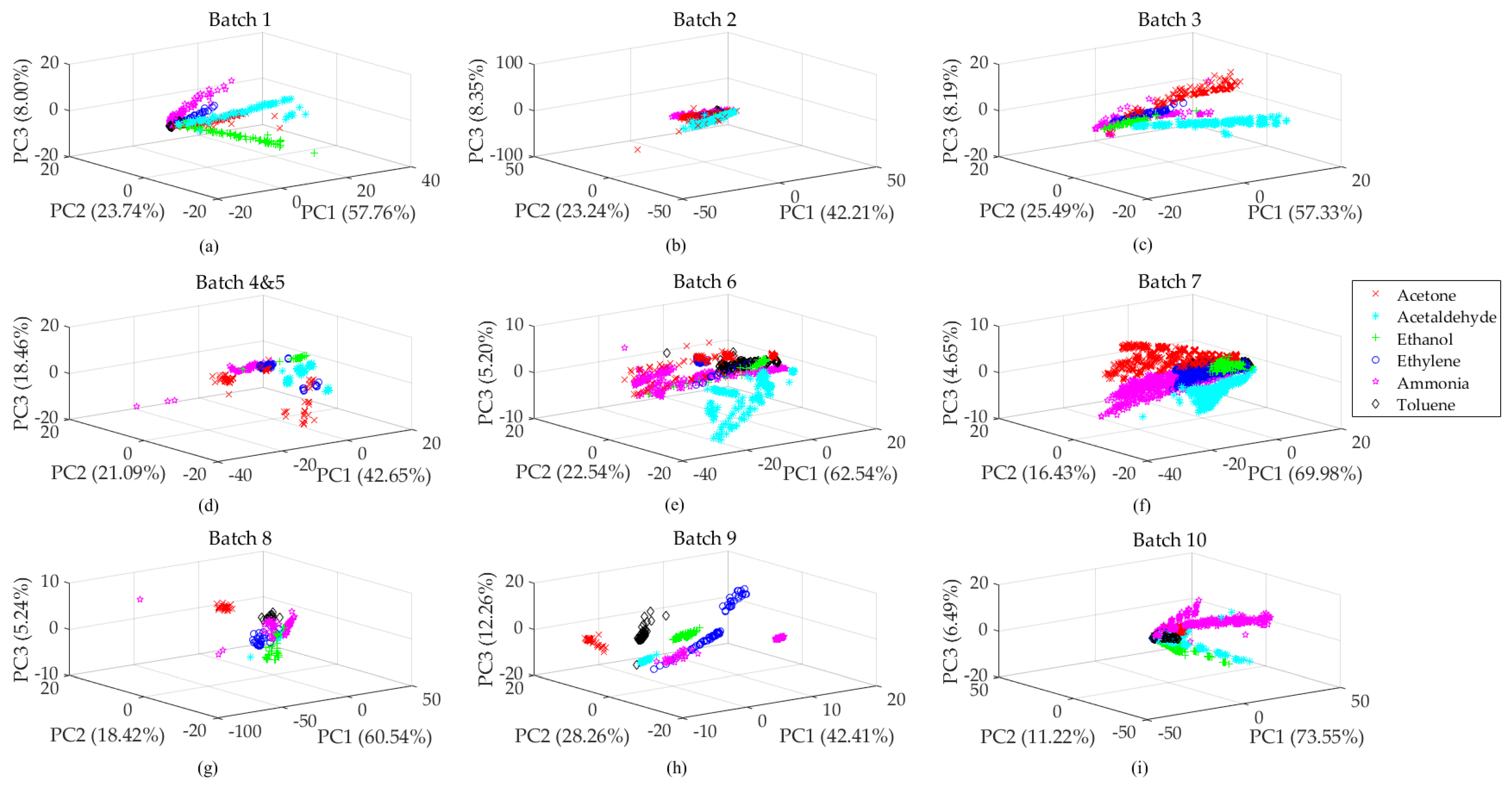
Dataset A was collected by an E-nose with 16 gas sensor arrays (four commercial series: TGS2600, TGS2602, TGS2610, and TGS2620) over 36 months. Considering that eight features were abstracted from each gas sensor response, one experiment can be denoted as a vector with 128 (16 × 8) dimensions. The acquisition time of an intact experiment took at least 300 s to complete, divided into 100 s for the gas injection phase and at least 200 s for the cleaning phase. Meanwhile, the experimental environment is controlled at a stable level (10% R.H., 25 ± 1 °C). Finally, a total of 13,910 samples were collected through the detection of six kinds of pure gaseous substances in the concentration range of 10–1000 ppmv (acetone, ammonia, acetaldehyde, ethylene, ethanol, and toluene). Especially, dataset A was divided into 10 batches by the authors according to the acquisition time-series. To accommodate E-nose drift compensation scenarios based on active learning, we integrated the small-size batches (batches 4 and 5) into a bigger-size one: batch 4&5. Figure 3 provides the sample distribution of the integrated nine batches. We can observe an obvious difference between two adjacent batches caused by gas sensor drift effects.
4.1.2. Dataset B
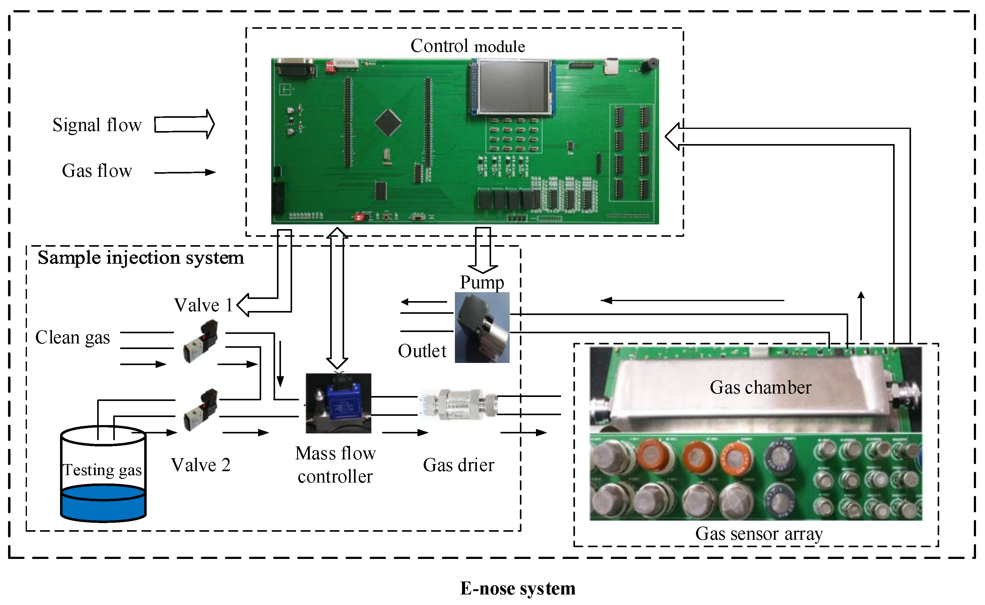
Dataset B was generated from our E-nose system over 4 months. As Figure 4 shows, the designed E-nose system consists of three parts: a gas sensor array, sample injection system, and control module. In an intact experiment, both the baseline and test stages lasted 3 min., maintaining the flow rate at 100 mL/min. Additionally, the cleaning stage lasted 6 min., maintaining the flow rate at 200 mL/min. For feature extraction, we used H0 and H to represent the steady-state voltage values of baseline and test stages, respectively. Thus, the abstracted feature of each gas sensor response can be expressed as follows:
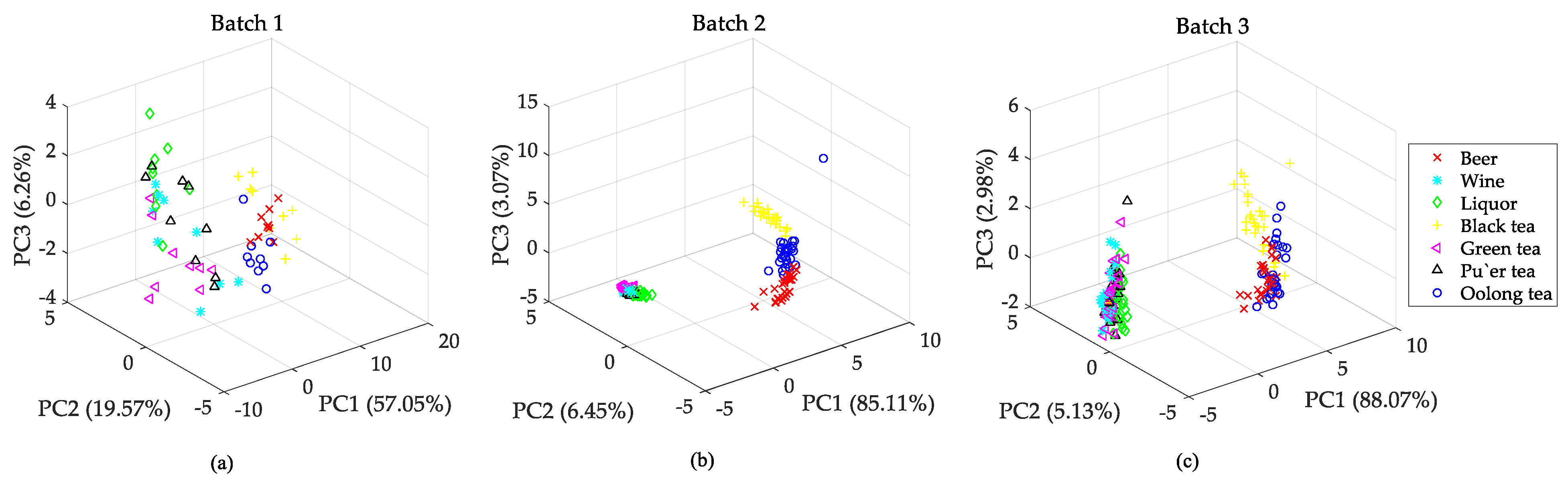
Considering the 32 gas sensors (listed in Table 2) in our E-nose system, each experiment can be represented as a 32-dimensional sample vector. We performed 441 experiments (30% R.H., 20 ± 1 °C) in 4 months on seven objects, including beer, wine, liquor, black tea, green tea, pu’er tea, and oolong tea. First, we mixed the original solution and distilled water at a volume ratio of 1:4. Especially, the original solution of tea samples was obtained by steeping 2 g of solid tea leaves and 200 mL of distilled water for 5 min. Then the mixed liquid was injected into a closed container and sealed for 10 min. Finally, the upper gases were used as experimental samples. Then, we collected these 441 samples as dataset B and divided them into three batches (63, 189, and 189 samples) in time order. Regarding dataset A, we plotted the PCA scatter points in Figure 5 to show the sample distribution of dataset B. We noticed that the distributions of batches 2 and 3 were similar owing to close acquisition time, while batch 1 showed significant variation on data distribution. Therefore, we can infer that drift calibration is needed for recognizing samples on varied distributions.
4.2. Experimental Setup
In order to simulate online drift scenarios of an E-nose, two experimental settings described in [22] were used as follows:
Setting 1 (long-term drift): Batch 1 was regarded as a training set, while the other batches were assumed to be drift data for successive testing.
Setting 2 (short-term drift): Batch K was regarded as a training set, while batch (K + 1) was assumed to be drift data for successive testing.
To validate the effectiveness of resisting the noisy-label problem, we compared the MPEGMM with other methods, including k-NN (k = 3, 3-NN) [31], classifiers vote (Vote) [32], disagreement measure (Disagree) [33], and bidirectional AL (BDAL) [34]. We assumed that the class labels from the expert were not completely correct during the AL process. Thus, we defined label-noise ratio (LNR) as follows:
where Nerr and N denote the numbers of mislabeled instances and drift calibration samples, respectively. We set three different LNRs (10%, 20%, and 30%) for both datasets A and B. Additionally, we selected about 5% samples from each testing batch (seen as unlabeled sample set) for labeling, while the remaining 95% samples were used for odor recognition.
In terms of classifier, we adopted a support vector machine (SVM), a popular and excellent classifier, for E-nose drift data classification. We chose the linear function as the kernel function of SVM due to the trade-off between higher performance and lower computational load. The penalty factor C was adjusted in the range of 10−3–103 with a two-phase grid optimization. In the first phase, we tested the C value at the points 10−3, 10−2, 10−1, 1, 10, 102, and 103 and chose two candidate intervals around the best point. Then, the decimus length of the chosen interval was used as the step length to explore the optimized C. After this two-phase optimization, we set C = 0.6 and 2 for datasets A and B, respectively. In addition, the parameter w of was determined through the Monte Carlo method, and the optimized values of w are presented in Table 3.
4.3. Recognition Comparison
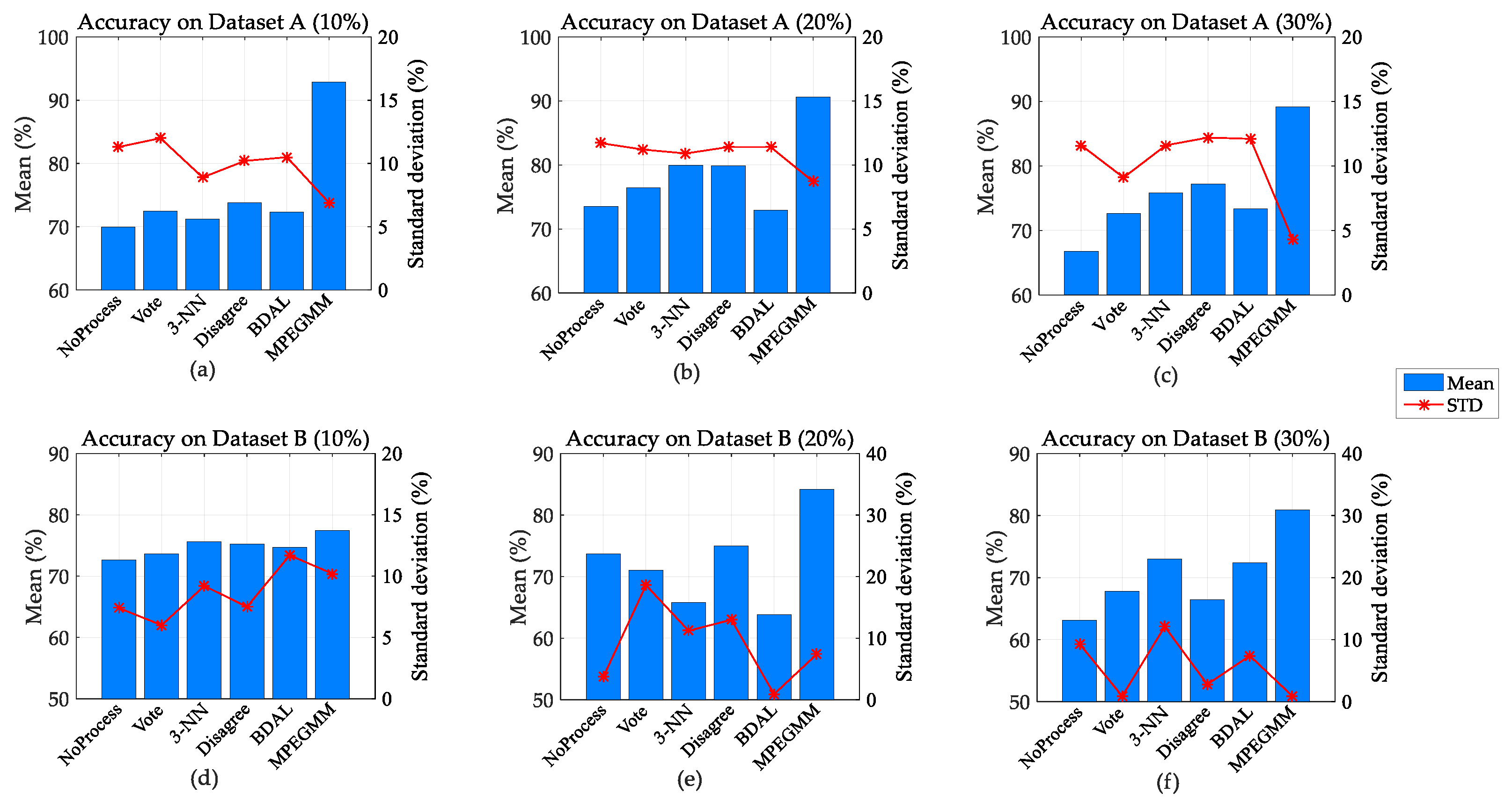
In this subsection, we aim to (1) demonstrate the superiority of the improved AL framework and (2) illustrate the effectiveness on mislabeled-instance selection of the proposed MPEGMM. Since the error-annotated labels were randomly set, we used the average value and standard deviation (Mean ± STD) by 10 repetitions to show the recognition performance of a certain method.
Figure 6 presents the accuracies of different methods under setting 1. We adopted the blue bars and red line with an asterisk to represent the mean and standard deviation, respectively. It is clear that no matter which LNR and dataset were adopted, the proposed MPEGMM would achieve the highest accuracy among all the tested methodologies. In Figure 6a–c, the accuracies of the MPEGMM are obviously higher than those of other reference methods on dataset A. The accuracy of the MPEGMM is always around 90% in all cases, while the accuracies of other paradigms are mostly less than 80%. In Figure 6d–f, we drew the accuracies on dataset B. The proposed MPEGMM was still the one with the highest accuracy among all the adopted methods. Furthermore, compared with the “NoProcess” strategy, the other methods demonstrated their effectiveness on recognition performance in most cases. Thus, we can discover that dealing with noisy labels in an AL procedure has a great impact on drift compensation.
As Table 4 and Table 5 show, we reported all recognition accuracies on datasets A and B under setting 2. The best one in each case is marked in bold. Obviously, the proposed MPEGMM is more efficient and robust than the other methodologies on both datasets A and B. In Table 4, the MPEGMM achieves the highest recognition accuracy of 97.90% in batch 6→7 with LNR = 10%. In Table 5, the MPEGMM still reaches the highest accuracy of 86.84% in batch 2→3 with LNR = 20%, which is 8.55% higher than the second-best one, 3-NN. As a result, we believe that the MPEGMM is an effective strategy for E-nose drift compensation in the AL-based calibration framework.
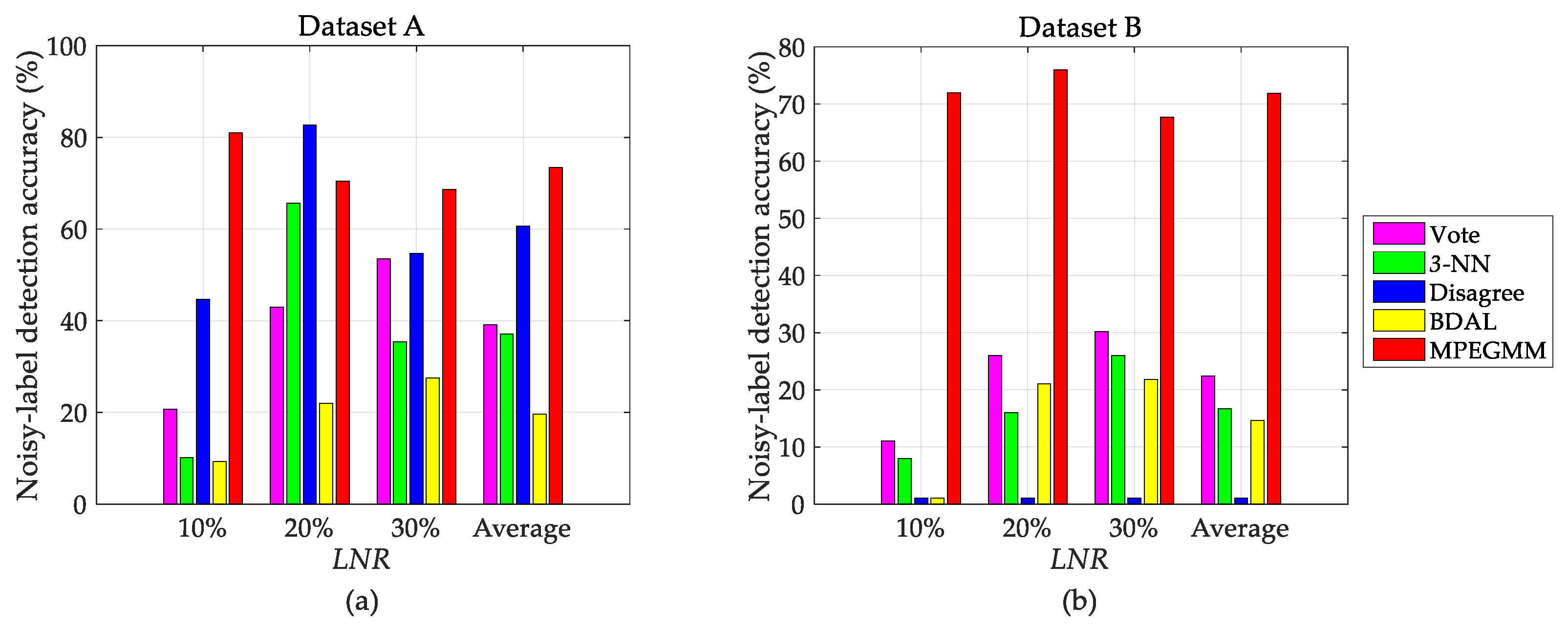
From the above results, the accuracy difference between the MPEGMM and other reference methods under setting 1 is significantly greater than the one under setting 2. This is because the number of mislabeled instances is gradually increased in the long-term scenario, which results in a slower decreasing of the classifier’s performance. In order to explain the reason why the MPEGMM achieves excellent recognition rates, we listed the noisy-label detection accuracies under setting 1. We drew the average accuracy calculated from batches 2–10 of dataset A in Figure 7a. The accuracies of the MPEGMM are apparently higher than those of other reference methods, except the point LNR = 20%. Although the Disagree strategy achieves the highest detection accuracy of around 83% at this point, the MPEGMM performs more stably under various LNRs. Meanwhile, in Figure 7b, we present the average detection accuracy of batches 2–3 from dataset B. The bars of the MPEGMM are on top compared with all other methods. Thus, we conclude that the proposed MPEGMM method can successfully identify more mislabeled instances. It is the key reason for making the updated classifier well performed under long-term drift.
4.4. Parameter Sensitivity
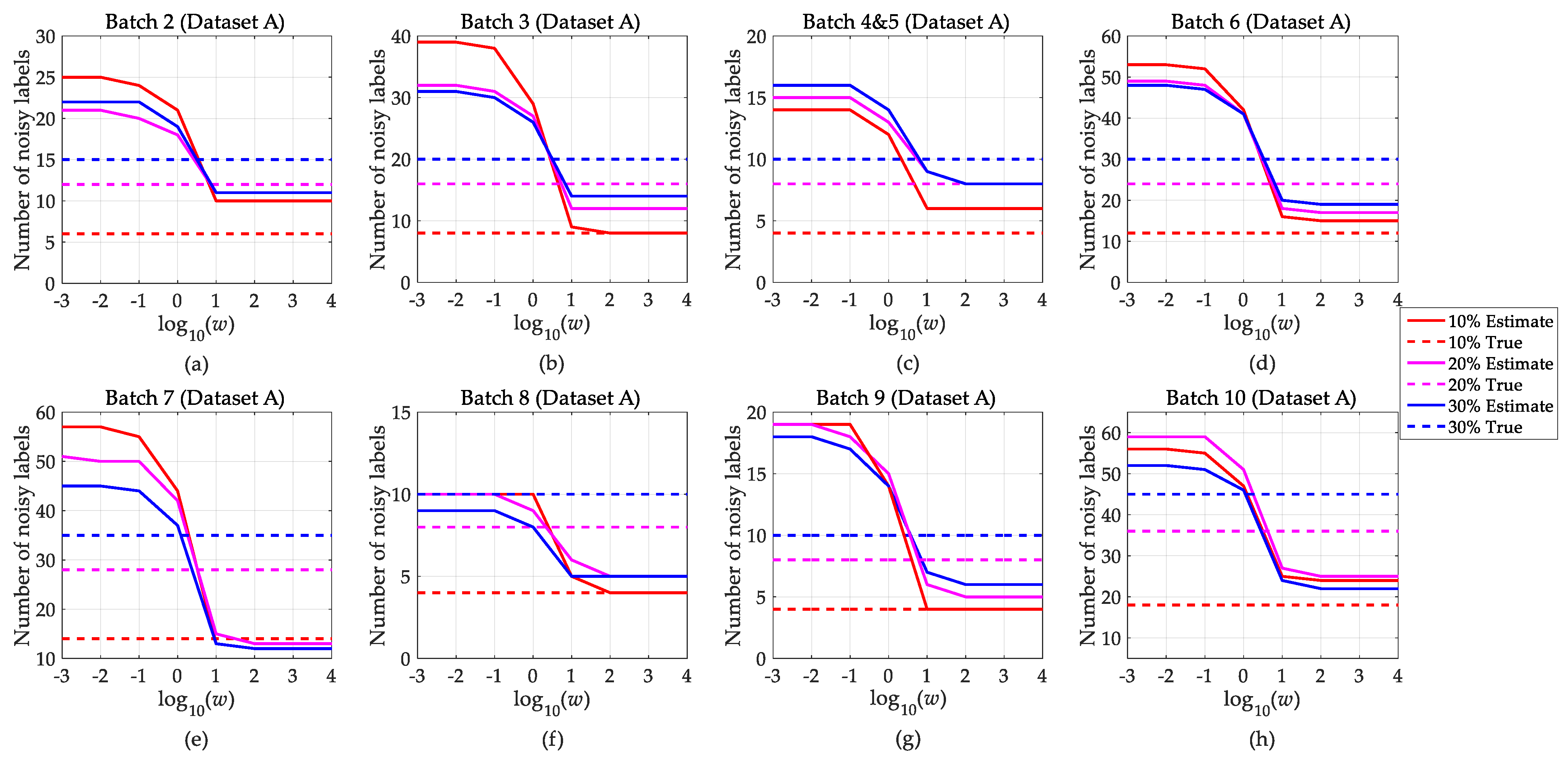
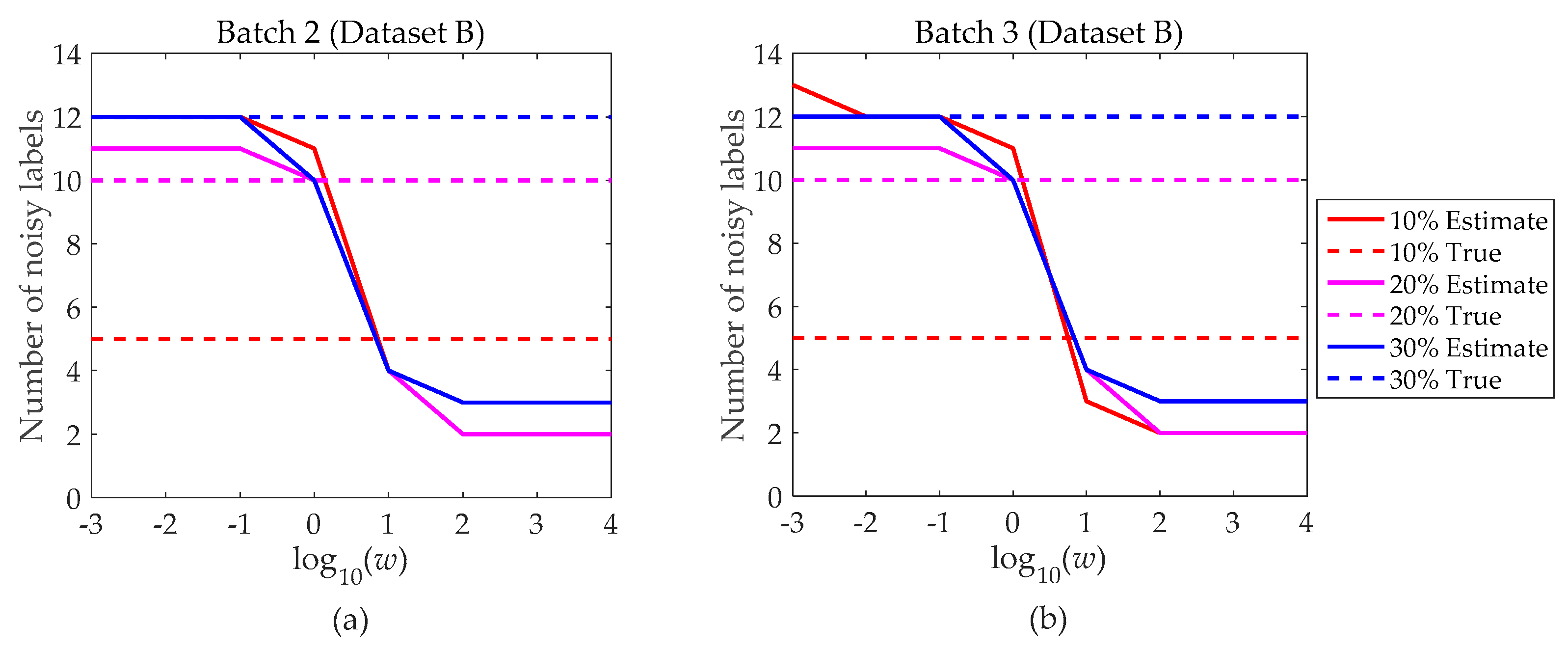
The purpose of the MPEGMM is to detect the mislabeled instances and deliver them to the expert for relabeling. Compared with other reference methods, the MPEGMM not only measures the mislabel probability of each selected instance but also estimates the total number of noisy labels in a drift calibration set. Especially, the estimated result is used in all tested methodologies to control the number of relabeled instances. If the estimated result is greater than the actual one, additional labeling costs will be considered. On the contrary, if the estimated number is smaller, some error labels will stay in the drift calibration set. It is necessary to observe the variation of parameter w controlling the estimated . Thus, we adjust w according to the set .
Figure 8 and Figure 9 show the parameter adjustment results of datasets A and B under setting 2. We use red, magenta, and blue to indicate LNRs of 10%, 20%, and 30%, respectively. For each color, a solid line and a dashed line represent the numbers of estimated and actual noisy labels, respectively. Then, the intersection of the solid line and dashed line corresponds to the range of optimal values. In Figure 8a–h, we can observe that the intersection points are mostly located in the range of 1–10 when LNR equals 20% and 30%. While LNR = 10%, the estimated quantity is slightly larger than the actual number, so we choose the closest interval (102, 104) as an optimized range. Accordingly, in Figure 9a,b, we can observe that 1–10 is the optimal parameter range when LNR equals 10% and 20%. For LNR = 30%. Basically, it is clear that the proposed MPEGMM can accurately estimate the total number of noisy labels at a proper interval of parameter w.
4.5. Computational Complexity
As Table 6 shows, we reported the average execution time of all tested methodologies by 10 repetitions on dataset A under setting 2. We can observe that Vote and Disagree have a similar execution time to identify one possible mislabeled instance, because they all need to train an SVM classifier on the same dataset. 3-NN takes a longer time since the size of the drift calibration set is larger and it needs to calculate the distance between the test instance and each drift calibration instance. For BDAL, we find that it consumes the longest time. It is reasonable that each time the label of a selected instance is changed, the training and testing process of the classifier must be redone by BDAL. On the contrary, the MPEGMM takes the least time among all the tested methodologies because the MPEGMM only calculates the increment of the expected entropy by the probability model instead of a complicated classifier training. In summary, we conclude that the computational complexity of the MPEGMM is superior to those of other reference methods.
5. Conclusions
In this paper, we proposed a class-label appraisal methodology, MPEGMM, for improving the active learning-based drift compensation framework under massive online data. The main idea of the MPEGMM is to measure the mislabel probability of each selected instance by a Gaussian mixture model. Furthermore, the MPEGMM estimates the labeling budget of noisy labels in a dataset and delivers the most valuable instances to the expert for relabeling. In the experiments, we simulated two representative scenarios, including long-term and short-term drift with two datasets. The MPEGMM achieves the highest recognition accuracy in most cases. The percentages 97.90% and 86.84% are, respectively, two best recognition scores on datasets A and B, which are 0.42% and 8.55% ahead of the best reference method. The key reason is that the MPEGMM can detect most of mislabeled instances correctly, thereby improving the recognition performance of the classifier. Moreover, the accuracy of the relabeling budget estimation is mainly affected by the parameter w, and the results show that 1–10 is a favorable range for relabeling times in common. Considering that the MPEGMM uses a probability model instead of a complicated classifier to estimate expected entropy increment, the computational time of the MPEGMM has been dramatically reduced compared with those of the other reference methods. Accordingly, the shortest average execution time of 0.299 s (on dataset A) is obtained by the MPEGMM for one-instance identification. Generally, it is a suitable choice to handle a noisy-label problem occurring in an online drift compensation of E-noses.
Reliable class label is an important issue in gas sensor drift compensation under massive online data. Besides our concern, multigas mixture, unknown interference, temperature, and humidity effects are some other challenging points in E-nose studies. A comprehensive method framework should be established to deal with these problems in the future.
Author Contributions
Conceptualization, J.C. (Jianhua Cao) and T.L.; methodology, J.C. (Jianhua Cao); software, J.C. (Jianhua Cao); validation, J.C. (Jianhua Cao) and T.L.; formal analysis, J.C. (Jianhua Cao) and T.L.; investigation, T.Y., X.Z. and H.W.; resources, T.L.; data curation, J.C. (Jianhua Cao); writing—original draft preparation, J.C. (Jianhua Cao); writing—review and editing, T.L.; visualization, J.C. (Jianhua Cao); supervision, T.L.; project administration, J.C. (Jianjun Chen); funding acquisition, T.L. All authors have read and agreed to the published version of the manuscript.
Funding
This work was supported by the Open Fund of Chongqing Key Laboratory of Bio-perception and Intelligent Information Processing under Grant No. 2019002.
Institutional Review Board Statement
Not applicable.
Informed Consent Statement
Not applicable.
Data Availability Statement
Not applicable.
Conflicts of Interest
The authors declare no conflict of interest.
References
- Gardner, J.W.; Bartlett, P.N.; Ye, M. A brief history of electronic noses. Sens. Actuators B Chem. 1994, 18, 211–220. [Google Scholar] [CrossRef]
- Wojnowski, W.; Majchrzak, T.; Dymerski, T.; Gbicki, J.; Namienik, J. Electronic noses: Powerful tools in meat quality assessment. Meat Sci. 2017, 131, 119–131. [Google Scholar] [CrossRef] [PubMed]
- Mumyakmaz, B.; Karabacak, K. An e-nose-based indoor air quality monitoring system: Prediction of combustible and toxic gas concentrations. Turk. J. Electr. Eng. Comput. Sci. 2015, 23, 729–740. [Google Scholar] [CrossRef]
- Na, J.; Jeon, K.; Lee, W.B. Toxic gas release modeling for real-time analysis using variational autoencoder with convolutional neural networks. Chem. Eng. Sci. 2018, 181, 68–78. [Google Scholar] [CrossRef]
- Aliaño-González, M.J.; Ferreiro-González, M.; Barbero, G.F.; Ayuso, J.; Álvarez, J.A.; Palma, M.; Barroso, C.G. An Electronic Nose Based Method for the Discrimination of Weathered Petroleum-Derived Products. Sensors 2018, 18, 2180. [Google Scholar] [CrossRef] [PubMed] [Green Version]
- Osowski, S.; Siwek, K. Mining Data of Noisy Signal Patterns in Recognition of Gasoline Bio-Based Additives using Electronic Nose. Metrol. Meas. Syst. 2017, 24. [Google Scholar] [CrossRef]
- Pashami, S.; Lilienthal, A.; Trincavelli, M. Detecting changes of a distant gas source with an array of mox gas sensors. Sensors 2012, 12, 16404–16419. [Google Scholar] [CrossRef] [PubMed] [Green Version]
- Maho, P.; Herrier, C.; Livache, T.; Comon, P.; Barthelmé, S. Real-time gas recognition and gas unmixing in robot applications. Sens. Actuators B Chem. 2020, 330, 129111. [Google Scholar] [CrossRef]
- Bartosz, S.; Jacek, N.; Jacek, G. Determination of Odour Interactions of Three-Component Gas Mixtures Using an Electronic Nose. Sensors 2017, 17, 2380. [Google Scholar] [CrossRef] [Green Version]
- Hudon, G.; Guy, C.; Hermia, J. Measurement of odor intensity by an electronic nose. J. Air Waste Manag. Assoc. 2000, 50, 1750–1758. [Google Scholar] [CrossRef]
- Yan, L.; Liu, J.; Shen, J.; Wu, C.; Gao, K. The Regular Interaction Pattern among Odorants of the Same Type and Its Application in Odor Intensity Assessment. Sensors 2017, 17, 1624. [Google Scholar] [CrossRef] [Green Version]
- Artursson, T.; Eklöv, T.; Lundström, I.; Mårtensson, P.; Sjöström, M.; Holmberg, M. Drift correction for gas sensors using multivariate methods. J. Chemom. 2000, 14, 711–723. [Google Scholar] [CrossRef]
- Ziyatdinov, A.; Marco, S.; Chaudry, A.; Persaud, K.; Caminal, P.; Perera, A. Drift compensation of gas sensor array data by common principal component analysis. Sens. Actuators B Chem. 2010, 146, 460–465. [Google Scholar] [CrossRef] [Green Version]
- Perera, A.; Papamichail, N.; Barsan, N.; Weimar, U.; Marco, S. On-line novelty detection by recursive dynamic principal component analysis and gas sensor arrays under drift conditions. IEEE Sens. J. 2006, 6, 770–783. [Google Scholar] [CrossRef]
- Padilla, M.; Perera, A.; Montoliu, I.; Chaudry, A.; Persaud, K.; Marco, S. Drift compensation of gas sensor array data by orthogonal signal correction. Chemom. Intell. Lab. Syst. 2010, 100, 28–35. [Google Scholar] [CrossRef]
- Laref, R.; Ahmadou, D.; Losson, E.; Siadat, M. Orthogonal signal correction to improve stability regression model in gas sensor systems. J. Sens. 2017, 2017, 1–8. [Google Scholar] [CrossRef] [Green Version]
- Kermit, M.; Tomic, O. Independent component analysis applied on gas sensor array measurement data. IEEE Sens. J. 2003, 3, 218–228. [Google Scholar] [CrossRef]
- Wang, H.; Zhao, Z.; Wang, Z.; Xu, G.; Wang, L. Independent component analysis based baseline drift interference suppression of portable spectrometer for optical electronic nose of internet of things. IEEE Trans. Industr. Inform. 2019, 99, 2698–2706. [Google Scholar] [CrossRef]
- Zhang, L.; Zhang, D. Domain adaptation extreme learning machines for drift compensation in E-nose systems. IEEE Trans. Instrum. Meas. 2015, 64, 1790–1801. [Google Scholar] [CrossRef] [Green Version]
- Liang, Z.; Tian, F.; Zhang, C.; Sun, H.; Song, A.; Liu, T. Improving the robustness of prediction model by transfer learning for interference suppression of electronic nose. IEEE Sens. J. 2017, 18, 1111–1121. [Google Scholar] [CrossRef]
- Ma, Z.; Luo, G.; Ke, Q.; Nan, W.; Niu, W. Weighted domain transfer extreme learning machine and its online version for gas sensor drift compensation in E-nose systems. Wirel. Commun. Mob. Comput. 2018, 2018, 1–17. [Google Scholar] [CrossRef] [Green Version]
- Vergara, A.; Vembu, S.; Ayhan, T.; Ryan, M.A.; Homer, M.L.; Huerta, R. Chemical gas sensor drift compensation using classifier ensembles. Sens. Actuators B Chem. 2012, 166, 320–329. [Google Scholar] [CrossRef]
- Liu, H.; Tang, Z. Metal oxide gas sensor drift compensation using a dynamic classifier ensemble based on fitting. Sensors 2013, 13, 9160–9173. [Google Scholar] [CrossRef] [Green Version]
- Verma, M.; Asmita, S.; Shukla, K.K. A regularized ensemble of classifiers for sensor drift compensation. IEEE Sens. J. 2016, 16, 1310–1318. [Google Scholar] [CrossRef]
- Yan, K.; Kou, L.; Zhang, D. Learning domain-invariant subspace using domain features and independence maximization. IEEE Trans. Cybern. 2018, 8, 288–299. [Google Scholar] [CrossRef] [PubMed]
- Liu, T.; Li, D.; Chen, J.; Chen, Y.; Yang, T.; Cao, J. Gas-sensor drift counteraction with adaptive active learning for an electronic nose. Sensors 2018, 18, 4028. [Google Scholar] [CrossRef] [PubMed] [Green Version]
- Wu, W.; Liu, Y.; Guo, M.; Wang, C.; Liu, X. A probabilistic model of active learning with multiple noisy oracles. Neurocomputing 2013, 118, 253–262. [Google Scholar] [CrossRef]
- Fang, M.; Zhu, X.; Li, B.; Ding, W.; Wu, X. Self-taught active learning from crowds. In Proceedings of the IEEE 12th International Conference on Data Mining, Brussels, Belgium, 10–13 December 2012; pp. 858–863. [Google Scholar] [CrossRef]
- Zhang, J.; Wu, X.; Shengs, V.S. Active learning with imbalanced multiple noisy labeling. IEEE Trans. Cybern. 2015, 45, 1095–1107. [Google Scholar] [CrossRef] [PubMed]
- Fang, M.; Zhu, X. Active learning with uncertain labeling knowledge. Pattern Recogn. Lett. 2014, 43, 98–108. [Google Scholar] [CrossRef]
- Wilson, D.L. Asymptotic properties of nearest neighbor rules using edited data. IEEE Trans. Syst. Man Cybern. 1972, SMC-2, 408–421. [Google Scholar] [CrossRef] [Green Version]
- Bouguelia, M.; Belaïd, Y.; Belaïd, A. Identifying and mitigating labelling errors in active learning. In Proceedings of the International Conference on Pattern Recognition Applications and Methods, Lisbon, Portugal, 10–12 January 2015; pp. 35–51. [Google Scholar] [CrossRef]
- Bouguelia, M.; Nowaczyk, S.; Santosh, K.C. Agreeing to disagree: Active learning with noisy labels without crowdsourcing. Int. J. Mach. Learn. Cybern. 2017, 9, 1307–1319. [Google Scholar] [CrossRef] [Green Version]
- Zhang, X.; Wang, S.; Yun, X. Bidirectional active learning: A two-way exploration into unlabeled and labeled data set. IEEE Trans. Neural Netw. Learn. Syst. 2015, 26, 3034–3044. [Google Scholar] [CrossRef] [PubMed]
- Shan, J.C.; Zhang, H.; Liu, W.K.; Liu, Q.B. Online active learning ensemble framework for drifted data streams. IEEE Trans. Neural Netw. Learn. Syst. 2018, 30, 486–498. [Google Scholar] [CrossRef] [PubMed]
Figure 1.
Active learning-based drift compensation.

Figure 2.
Improved AL-based drift calibration framework.

Figure 3.
Data distribution of dataset A. (a) Distribution of batch 1, (b) distribution of batch 2, (c) distribution of batch 3, (d) distribution of batch 4&5, (e) distribution of batch 6, (f) distribution of batch 7, (g) distribution of batch 8, (h) distribution of batch 9, (i) distribution of batch 10.

Figure 4.
Structure of our E-nose system.

Figure 5.
Data distribution of dataset B. (a) Distribution of batch 1, (b) distribution of batch 2, (c) distribution of batch 3.
Figure 5.
Data distribution of dataset B. (a) Distribution of batch 1, (b) distribution of batch 2, (c) distribution of batch 3.

Figure 6.
Accuracy under setting 1. (a) Accuracy on dataset A with LNR = 10%; (b) accuracy on dataset A with label-noise ratio (LNR) = 20%; (c) accuracy on dataset A with LNR = 30%; (d) accuracy on dataset B with LNR = 10%; (e) accuracy on dataset B with LNR = 20%; (f) accuracy on dataset B with LNR = 30%.

Figure 7.
Noisy-label detection accuracy with LNR under setting 1. (a) Detection accuracy on dataset A; (b) detection accuracy on dataset B.
Figure 7.
Noisy-label detection accuracy with LNR under setting 1. (a) Detection accuracy on dataset A; (b) detection accuracy on dataset B.

Figure 8.
Estimated number of noisy labels with w (dataset A). (a) Noisy number of batch 2, (b) noisy number of batch 3, (c) noisy number of batch 4&5, (d) noisy number of batch 6, (e) noisy number of batch 7, (f) noisy number of batch 8, (g) noisy number of batch 9; (h) noisy number of batch 10.
Figure 8.
Estimated number of noisy labels with w (dataset A). (a) Noisy number of batch 2, (b) noisy number of batch 3, (c) noisy number of batch 4&5, (d) noisy number of batch 6, (e) noisy number of batch 7, (f) noisy number of batch 8, (g) noisy number of batch 9; (h) noisy number of batch 10.

Figure 9.
Estimated number of noisy labels with w (dataset B). (a) Noisy number of batch 2; (b) noisy number of batch 3.
Figure 9.
Estimated number of noisy labels with w (dataset B). (a) Noisy number of batch 2; (b) noisy number of batch 3.


Table 1.
Comparison between mislabel probability estimation method based on a Gaussian mixture model (MPEGMM) and other methods.
Table 1.
Comparison between mislabel probability estimation method based on a Gaussian mixture model (MPEGMM) and other methods.
| Method | Accuracy | Adaptation | Cost |
|---|---|---|---|
| Multiple experts [27,28,29] | High | High | High |
| k-NN [31] | Mid | Mid | Mid |
| Disagreement measure [32,33] | Mid | Low | Low |
| Bidirectional AL [34] | Mid | Mid | Mid |
| MPEGMM | High | High | Low |
Table 2.
Gas sensor details of our E-nose system.
| Model | Type | Test Objects | Model | Type | Test Objects |
|---|---|---|---|---|---|
| TGS800 | Metal oxide | Smog | MQ-7B | Metal oxide | Carbon monoxide |
| TGS813 | Methane, ethane, propane | MQ131 | Ozone | ||
| TGS816 | Inflammable gas | MQ135 | Ammonia, sulfide, benzene | ||
| TGS822 | Ethanol | MQ136 | Sulfuretted hydrogen | ||
| TGS2600 | Hydrogen, methane | MP-3B | Ethanol | ||
| TGS2602 | Methylbenzene, ammonia | MP-4 | Methane | ||
| TGS2610 | Inflammable gas | MP-5 | Propane | ||
| TGS2612 | Methane | MP-135 | Air pollutant | ||
| TGS2620 | Ethanol | MP-901 | Cigarettes, ethanol | ||
| TGS2201A | Gasoline exhaust | WSP2110 | Formaldehyde, benzene | ||
| TGS2201B | Carbon monoxide | WSP5110 | Freon | ||
| GSBT11 | Formaldehyde, benzene | SP3-AQ2-01 | Organic compounds | ||
| MQ-2 | Ammonia, sulfide | ME2-CO | Electrochemical | Carbon monoxide | |
| MQ-3B | Ethanol | ME2-CH2O | Formaldehyde | ||
| MQ-4 | Methane | ME2-O2 | Oxygen | ||
| MQ-6 | Liquefied petroleum gas | TGS4161 | Solid electrolyte | Carbon monoxide |
Table 3.
Parameter values of the MPEGMM.
| Parameter | Dataset A | Dataset B | ||||
|---|---|---|---|---|---|---|
| label-noise ratio (LNR) | 10% | 20% | 30% | 10% | 20% | 30% |
| w | 100 | 5 | 5 | 5 | 1 | 0.1 |
Table 4.
Accuracy on dataset A under setting 2 (%).
| LNR | Method | 1→2 | 2→3 | 3→4&5 | 4&5→6 | 6→7 | 7→8 | 8→9 | 9→10 |
|---|---|---|---|---|---|---|---|---|---|
| 10% | NoProcess | 87.98 ± 9.40 | 92.14 ± 9.32 | 85.44 ± 6.70 | 93.49 ± 2.37 | 94.17 ± 3.33 | 86.57 ± 5.59 | 90.16 ± 4.66 | 89.48 ± 4.35 |
| Vote | 93.01 ± 7.89 | 90.98 ± 8.28 | 85.82 ± 7.01 | 92.90 ± 3.02 | 97.48 ± 1.32 | 86.57 ± 5.59 | 90.25 ± 4.76 | 89.09 ± 4.57 | |
| 3-NN | 87.98 ± 9.40 | 91.47 ± 8.35 | 85.44 ± 6.70 | 93.61 ± 2.13 | 96.13 ± 2.57 | 87.04 ± 6.04 | 90.16 ± 4.62 | 88.63 ± 4.83 | |
| Disagree | 89.45 ± 9.66 | 95.54 ± 1.76 | 85.47 ± 6.73 | 93.39 ± 3.00 | 93.83 ± 3.11 | 91.24 ± 1.75 | 90.75 ± 4.82 | 89.89 ± 5.25 | |
| BDAL | 88.22 ± 9.80 | 92.72 ± 8.55 | 85.88 ± 6.77 | 93.03 ± 2.27 | 96.13 ± 2.39 | 86.57 ± 5.59 | 90.16 ± 4.66 | 89.48 ± 3.80 | |
| MPEGMM | 94.25 ± 4.53 | 97.40 ± 1.77 | 90.19 ± 5.24 | 95.28 ± 1.95 | 97.90 ± 2.23 | 90.62 ± 3.05 | 90.34 ± 5.05 | 90.20 ± 4.43 | |
| 20% | NoProcess | 85.21 ± 10.85 | 82.46 ± 7.56 | 92.70 ± 6.96 | 76.54 ± 2.47 | 91.91 ± 6.43 | 84.54 ± 2.29 | 89.16 ± 12.45 | 56.21 ± 6.61 |
| Vote | 90.82 ± 12.74 | 94.43 ± 5.36 | 91.89 ± 6.08 | 94.72 ± 3.98 | 95.24 ± 1.29 | 86.95 ± 4.75 | 91.84 ± 11.90 | 79.93 ± 6.87 | |
| 3-NN | 89.86 ± 14.27 | 94.55 ± 6.77 | 91.82 ± 6.67 | 96.51 ± 1.02 | 95.82 ± 2.59 | 85.69 ± 3.80 | 91.53 ± 12.00 | 80.38 ± 6.67 | |
| Disagree | 91.44 ± 6.51 | 97.37 ± 3.75 | 95.22 ± 2.68 | 94.18 ± 1.83 | 95.32 ± 1.92 | 84.54 ± 4.53 | 91.16 ± 11.91 | 79.01 ± 7.42 | |
| BDAL | 91.64 ± 7.50 | 85.66 ± 6.74 | 90.75 ± 6.82 | 94.87 ± 3.39 | 96.31 ± 1.49 | 85.84 ± 5.00 | 91.74 ± 11.90 | 79.84 ± 7.81 | |
| MPEGMM | 91.38 ± 13.25 | 97.62 ± 2.45 | 93.58 ± 4.39 | 96.27 ± 1.28 | 97.89 ± 0.41 | 88.48 ± 3.93 | 91.56 ± 12.12 | 82.18 ± 4.65 | |
| 30% | NoProcess | 67.55 ± 13.99 | 77.11 ± 3.01 | 85.60 ± 6.36 | 91.85 ± 2.97 | 91.73 ± 5.53 | 75.66 ± 4.94 | 85.29 ± 12.87 | 80.84 ± 7.87 |
| Vote | 87.27 ± 13.23 | 92.22 ± 7.67 | 93.08 ± 3.36 | 95.06 ± 2.04 | 92.33 ± 4.52 | 84.34 ± 7.03 | 91.40 ± 4.87 | 80.75 ± 7.96 | |
| 3-NN | 89.60 ± 11.27 | 95.07 ± 4.11 | 92.42 ± 3.91 | 95.84 ± 1.86 | 94.54 ± 4.96 | 84.34 ± 6.66 | 91.95 ± 7.68 | 83.48 ± 6.48 | |
| Disagree | 85.82 ± 6.19 | 90.82 ± 8.16 | 84.94 ± 7.61 | 91.64 ± 3.51 | 93.22 ± 4.37 | 75.95 ± 4.73 | 85.29 ± 12.87 | 83.12 ± 7.11 | |
| BDAL | 91.74 ± 4.35 | 91.27 ± 7.17 | 87.01 ± 7.30 | 92.69 ± 2.42 | 91.38 ± 5.28 | 80.58 ± 6.91 | 92.51 ± 4.87 | 80.88 ± 8.30 | |
| MPEGMM | 91.89 ± 4.93 | 94.77 ± 4.12 | 89.78 ± 7.85 | 96.59 ± 2.31 | 94.32 ± 3.36 | 85.88 ± 3.60 | 93.03 ± 7.73 | 83.59 ± 8.68 |
Table 5.
Accuracy on dataset B under setting 2 (%).
| LNR | 10% | 20% | 30% | |||
|---|---|---|---|---|---|---|
| Batch ID | 1→2 | 2→3 | 1→2 | 2→3 | 1→2 | 2→3 |
| NoProcess | 70.19 ± 4.80 | 74.34 ± 10.23 | 69.55 ± 8.63 | 77.63 ± 13.03 | 63.57 ± 9.33 | 64.74 ± 4.84 |
| Vote | 70.19 ± 4.80 | 79.61 ± 2.79 | 70.06 ± 7.90 | 77.63 ± 16.75 | 69.74 ± 7.30 | 71.71 ± 5.34 |
| 3-NN | 73.57 ± 3.23 | 74.34 ± 10.23 | 71.36 ± 6.50 | 78.29 ± 15.82 | 71.43 ± 7.98 | 70.66 ± 6.30 |
| Disagree | 71.56 ± 3.65 | 74.34 ± 10.23 | 72.14 ± 6.42 | 77.63 ± 13.03 | 68.31 ± 9.03 | 64.74 ± 4.84 |
| BDAL | 70.19 ± 4.80 | 74.34 ± 10.23 | 69.94 ± 8.62 | 76.97 ± 13.96 | 66.10 ± 10.16 | 67.50 ± 6.60 |
| MPEGMM | 74.16 ± 4.78 | 82.24 ± 4.65 | 73.18 ± 8.21 | 86.84 ± 11.16 | 72.92 ± 5.79 | 75.79 ± 5.96 |
Table 6.
Average time of identifying one instance (second).
| Method | 1→2 | 2→3 | 3→4&5 | 4&5→6 | 6→7 | 7→8 | 8→9 | 9→10 | Average |
|---|---|---|---|---|---|---|---|---|---|
| Vote | 0.313 | 0.862 | 0.661 | 0.159 | 0.510 | 3.783 | 0.161 | 0.251 | 0.838 |
| 3-NN | 1.205 | 1.111 | 1.161 | 1.178 | 2.644 | 1.726 | 0.927 | 0.952 | 1.363 |
| Disagree | 0.381 | 0.934 | 0.912 | 0.249 | 2.182 | 3.872 | 0.179 | 0.467 | 1.147 |
| BDAL | 1.377 | 3.069 | 2.647 | 1.088 | 8.305 | 10.814 | 0.510 | 1.725 | 3.692 |
| MPEGMM | 0.296 | 0.319 | 0.307 | 0.286 | 0.396 | 0.197 | 0.153 | 0.437 | 0.299 |
Publisher’s Note: MDPI stays neutral with regard to jurisdictional claims in published maps and institutional affiliations. |
© 2021 by the authors. Licensee MDPI, Basel, Switzerland. This article is an open access article distributed under the terms and conditions of the Creative Commons Attribution (CC BY) license (https://creativecommons.org/licenses/by/4.0/).
Share and Cite
MDPI and ACS Style
Cao, J.; Liu, T.; Chen, J.; Yang, T.; Zhu, X.; Wang, H. Drift Compensation on Massive Online Electronic-Nose Responses. Chemosensors 2021, 9, 78. https://0-doi-org.brum.beds.ac.uk/10.3390/chemosensors9040078
AMA Style
Cao J, Liu T, Chen J, Yang T, Zhu X, Wang H. Drift Compensation on Massive Online Electronic-Nose Responses. Chemosensors. 2021; 9(4):78. https://0-doi-org.brum.beds.ac.uk/10.3390/chemosensors9040078
Chicago/Turabian StyleCao, Jianhua, Tao Liu, Jianjun Chen, Tao Yang, Xiuxiu Zhu, and Hongjin Wang. 2021. "Drift Compensation on Massive Online Electronic-Nose Responses" Chemosensors 9, no. 4: 78. https://0-doi-org.brum.beds.ac.uk/10.3390/chemosensors9040078
Note that from the first issue of 2016, this journal uses article numbers instead of page numbers. See further details here.