
Photoluminescent Metal Complexes and Materials as Temperature Sensors—An Introductory Review

Chemical Physics Laboratory, Concordia University, 1530 Concordia West, Irvine, CA 92612, USA
*
Author to whom correspondence should be addressed.
Chemosensors 2021, 9(5), 109; https://0-doi-org.brum.beds.ac.uk/10.3390/chemosensors9050109
Submission received: 31 March 2021
/
Revised: 30 April 2021
/
Accepted: 7 May 2021
/
Published: 14 May 2021
(This article belongs to the Special Issue Luminescent Metal Complexes as Sensors)
Abstract
:Temperature is a fundamental physical quantity whose accurate measurement is of critical importance in virtually every area of science, engineering, and biomedicine. Temperature can be measured in many ways. In this pedagogically focused review, we briefly discuss various standard contact thermometry measurement techniques. We introduce and touch upon the necessity of non-contact thermometry, particularly for systems in extreme environments and/or in rapid motion, and how luminescence thermometry can be a solution to this need. We review the various aspects of luminescence thermometry, including different types of luminescence measurements and the numerous materials used as luminescence sensors. We end the article by highlighting other physical quantities that can be measured by luminescence (e.g., pressure, electric field strength, magnetic field strength), and provide a brief overview of applications of luminescence thermometry in biomedicine.
Keywords:
non-contact; sensor; thermometer; luminescence; phosphorescence; fluorescence; pressure; oxygen; magnetic-field; electric-field1. Introduction
The need to measure temperature is ubiquitous in science, engineering, and biomedicine. The methods by which temperature may now be measured in the 21st century span an incredibly diverse spectrum of technologies, techniques, and phenomena [1]. Moreover, many of the techniques used to measure temperature can also be used, often with simple and straightforward modifications, to measure pressure and other properties such as electric field, magnetic field, and dissolved oxygen concentration in water or blood. Temperatures to be measured extend from the ultra-cold μK range (cryostat cooled copper) to the ~4-Kelvin range (liquid helium) to the ~55,000-Kelvin range (hottest stars) [2]. The 0 °C to 100 °C range (273.15 K to 373.15 K, water freezing point to boiling point) is of special interest in that, with rare exceptions, all life processes on planet Earth operate within this range. Temperature measurement techniques must be scaled to the physical size and the mass of object. For small objects in particular, such has single biological cells, great care must be taken to insure that the temperature measurement technique is not significantly perturbing the temperature of what is being measured. In some applications, multiple temperature measurements must be made in a fraction of a second. In other applications, it becomes necessary to allow a long period of time for the thermometer to become thermally equilibrated with the sample whose temperature is to be measured. A brief review of some common and not-so-common temperature measurement devices and techniques follows to set the stage for a detailed discussion of luminescence-based thermometry.
2. Background and Operating Principles of Some Common Thermometer Types
2.1. Liquid-in-Glass Thermometer
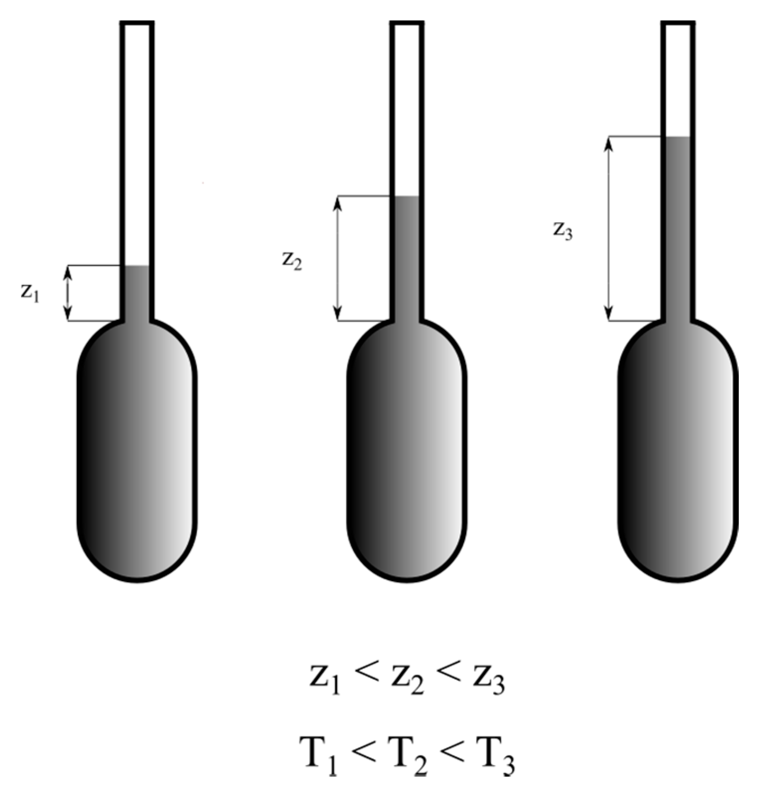
The classic temperature measurement device is the liquid filled bulb and capillary thermometer (Figure 1) [1]. The total volume of the liquid in the bulb and capillary—typically mercury or alcohol to which a dye has been added to increase visibility—increases with increasing temperature, forcing the liquid up the capillary to which a linear scale marked off in degrees °C is attached or inscribed.
The thermometer bulb and capillary are constructed out of a borosilicate glass with a low thermal expansion coefficient (e.g., Pyrex) to ensure that the bulb volume and the capillary internal diameter do not change appreciably with a change in temperature. As the liquid in the bulb and capillary heats up, the liquid rises up in the capillary to a distance, z, measured with respect to a reference distance, z0. The total volume and thus the temperature may then be expressed as a linear function of z:
where a and b are constants. Note that Vtot = Vbulb + Vcapillary = Vbulb + πr2z where z is the liquid height in the capillary and r is the inside radius of the capillary.
T = f(z) = az + b
2.2. Gas Thermometer
In a gas thermometer (Figure 2), a known amount of an inert gas (e.g., nitrogen or helium) is placed in a sealed bulb to which a pressure gauge is attached via a small-diameter capillary tube where [1].
V = Vbulb >> Vcapillary
Solving the ideal gas law for temperature yields
where n is the number of moles of gas, p is the gas pressure, V is the total internal volume of the system, and R is the gas constant (8.3144 J/mol K). Assuming the ideal gas law holds, Equation (3) shows that the temperature T is a linear function of the pressure p. As in the case of the liquid capillary-bulb thermometer, the internal volume of the gas capillary-bulb unit is assumed be temperature independent.
T = pV/nR = (V/nR)p
2.3. Thermocouple Thermometer
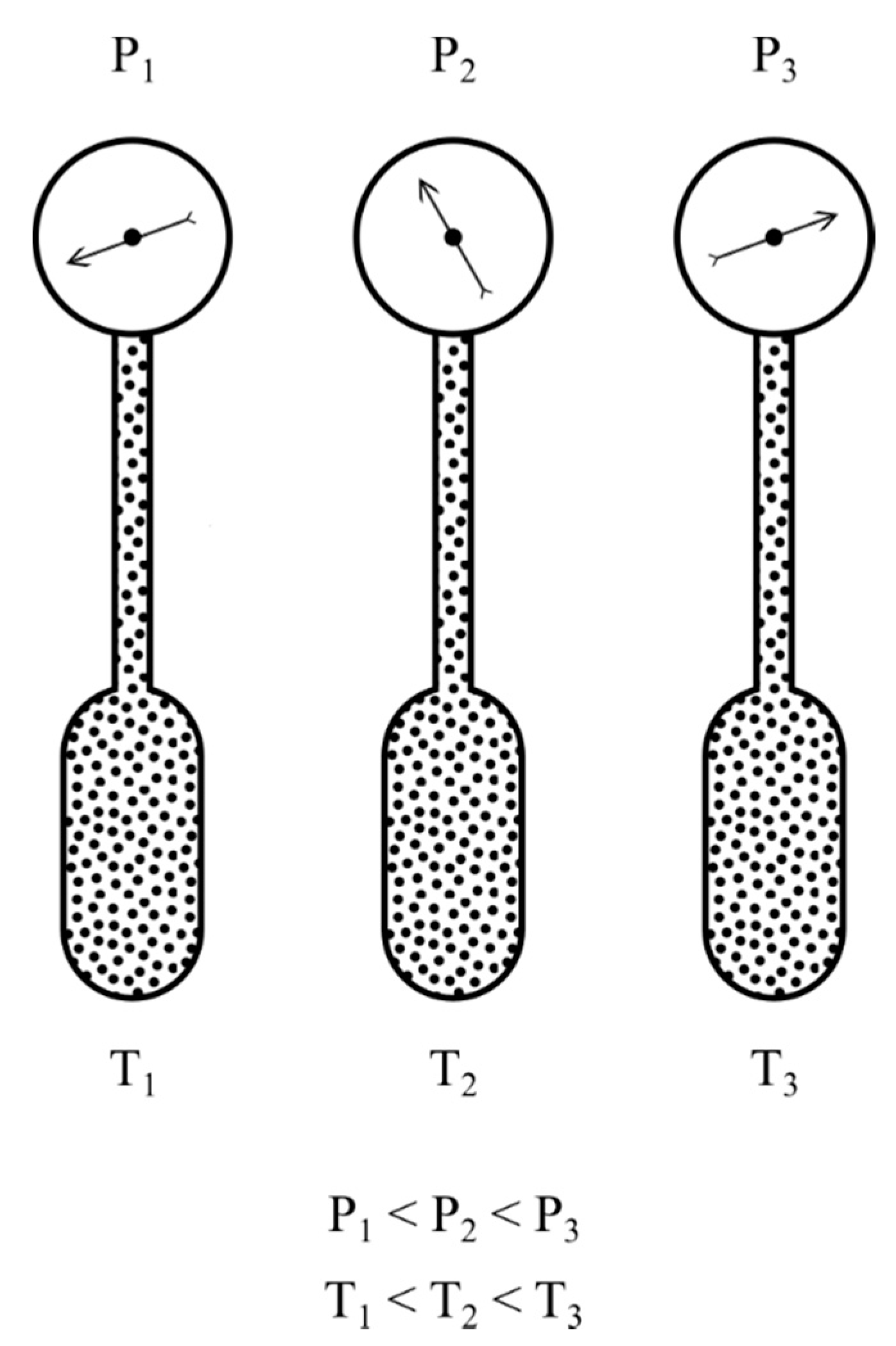
Thermocouple thermometers (Figure 3) represent an entirely different approach to temperature measurement [1]. Two wires comprised of dissimilar metals (e.g., copper and a copper-nickel alloy called Constantan) are joined together at one end to form a thermocouple junction.
At the other end, these wires are connected to the terminals of an accurate high-impedance digital multimeter set to read volts. As expressed by the function f, the voltage ΔV changes in a well-defined way as temperature changes [1].
T = f(V)
In actual practice, it proves to be useful to set up two junctions, a sample junction and a reference junction, in opposition to one another to yield a differential voltage ΔV = Vsample − VReference,
which is a well-defined function of temperature as described by the function f. A commonly used constant temperature bath for the reference junction is the 0.00 °C (273.15 K) distilled water-ice mixture [1].
T = f(ΔV)
2.4. Resistance Temperature Devices
Resistance temperature devices (RTDs) are based upon the known temperature-dependence of the electrical resistance R of a resistor
T = f(R)
2.5. Thermometer Overview
Each of the thermometers described above operates on the same general principle; a function f is established, which connects the input to the function—a height z, a pressure p, a voltage difference ΔV, an electrical resistance R, or spectroscopic parameters such as wavelength λ, wavenumber , spectral bandwidth , intensity I, or lifetime τ, rise time tr —to the temperature T [1]. The function f must be responsive to temperature. It is nice but not necessary for f to be linear as in the cases of the bulb and capillary thermometer and the “ideal” gas thermometer. The function f should, however, be smoothly increasing or smoothly decreasing over the entire operating range of the thermometer. The explicit form of f for a given thermometer is obtained by collecting a T vs. x data set where x (e.g., capillary liquid column height z or pressure p) is the value of the property at a known calibration temperature T. This data set may then be fitted to a least squares polynomial to yield a numerical power series expression for the function f:
as described by the temperature-dependent property x and the coefficients a, b, c, d, … However, a disadvantage of this approach is the loss of insight into the mechanistic details of the thermometer.
T = a + bx + cx2 + dx3 +...
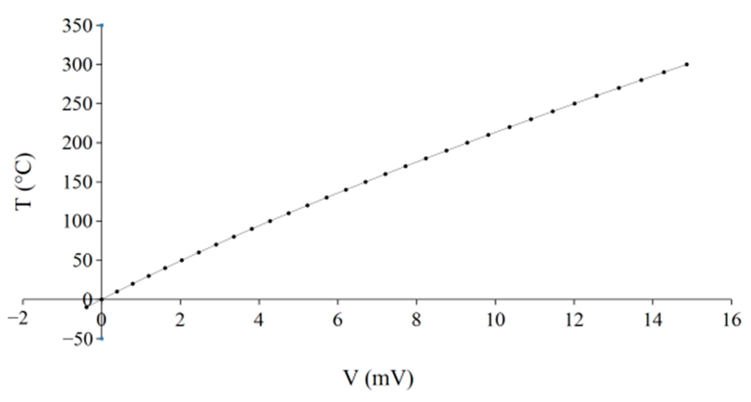
Consider, for example, a thermometer based upon a copper-Constantan Type T thermocouple equipped with a sample junction, a water-ice reference junction, and a high-impedance digital multimeter set to measure voltage (see Figure 3). The desired operating range of this thermometer is chosen to be 300–320 K. Data from a Type T thermocouple standard data table [3] over the range 280–340 K, which extends above and below the desired operating range, is fit to the polynomial in Equation (7) as shown in Figure 5.
3. Luminescence Non-Contact Thermometry
3.1. Luminescence-Based Thermometers
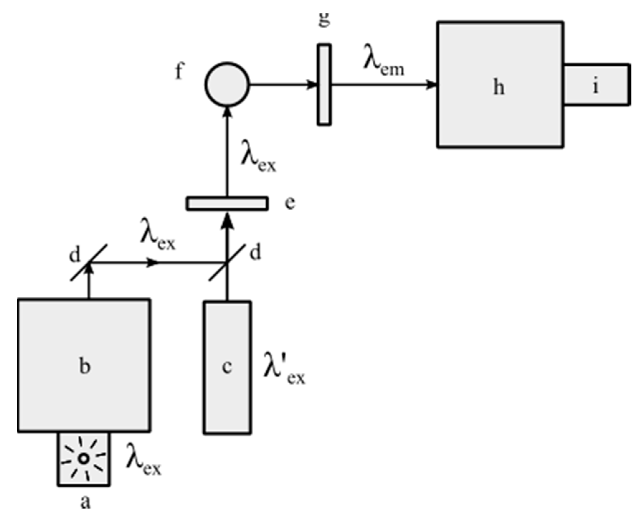
The diverse phenomena associated with luminescence or light emission—in particular, photoluminescence, the luminescence from a sample induced by higher energy excitation photons—lend themselves to a wide variety of thermometric techniques and applications [4]. The advent of laser excitation sources and sensitive, accurate, energy-resolved, and time-resolved photon detection systems, has ushered in a new era of luminescence-based thermometry [4]. Moreover, many of these luminescence-based temperature measuring techniques can be implemented on standard, commercially available fluorimeters (i.e., luminescence spectrophotometers) [4] of modest spectral resolution (Figure 6) that are outfitted with suitable optical systems for injecting light into the spectrophotometer for measurement and analysis and that make use of straightforward combinations of lenses, mirrors, and fiber optic cables.
3.2. Practical Considerations: Surmounting Challenges in Temperature Measurement
Assuming a thermometer is robust in design and accurately covers the temperature range of interest, it still may not be a suitable thermometer for its intended use. The wires of a thermocouple can be destroyed in a high temperature environment or an acidic environment. In a high magnetic field and/or electric field environment, a thermocouple or other electrically-based thermometer type may give a spurious output [1]. The large size of a liquid or gas thermometer bulb or junction may preclude measuring the temperatures of small samples. To make accurate temperature maps of small objects such as a computer chip or a single biological cell, the temperature probe itself (e.g., a laser beam diameter) must be small enough to give the desired thermal resolution [4]. Many thermometer measurement techniques are based upon physical contact between the thermometer sensor and the sample. This becomes virtually impossible if the sample is in rapid motion.
3.3. Luminescence-Based Temperature Measurements
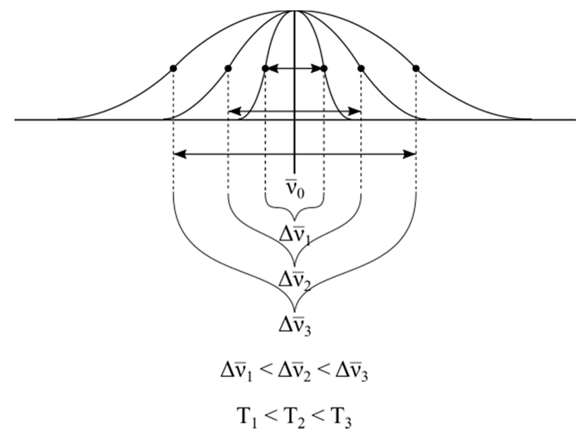
Numerous exciting new developments in thermometry involve the use of temperature-dependent photoluminescence phenomena as indicators of temperature [4]. In some cases, classic temperature measurement techniques based upon an analysis luminescence induced by a broad-band excitation source, are transformed by switching to monochromatic laser excitation. A notable example involves the extraction of sample temperature from laser-induced thermally broadened Doppler luminescence spectral profiles, as shown in Figure 7 [5]. The temperature T of the luminescing sample is determined by inserting the measured spectral bandwidth of the emission at together with the measured band maximum and solving for T in Equation (8)
In Equation (8), is the full width at half maximum of the luminescence band in wavenumbers (cm−1), k is the Boltzmann constant, m is the mass of a single emitting atom or molecule in the sample, c is the speed of light, and is the experimentally determined emission band maximum expressed in wavenumbers, and T is the absolute temperature of the sample.
3.4. High Resolution, Non-Contact Luminescence-Based Thermometry
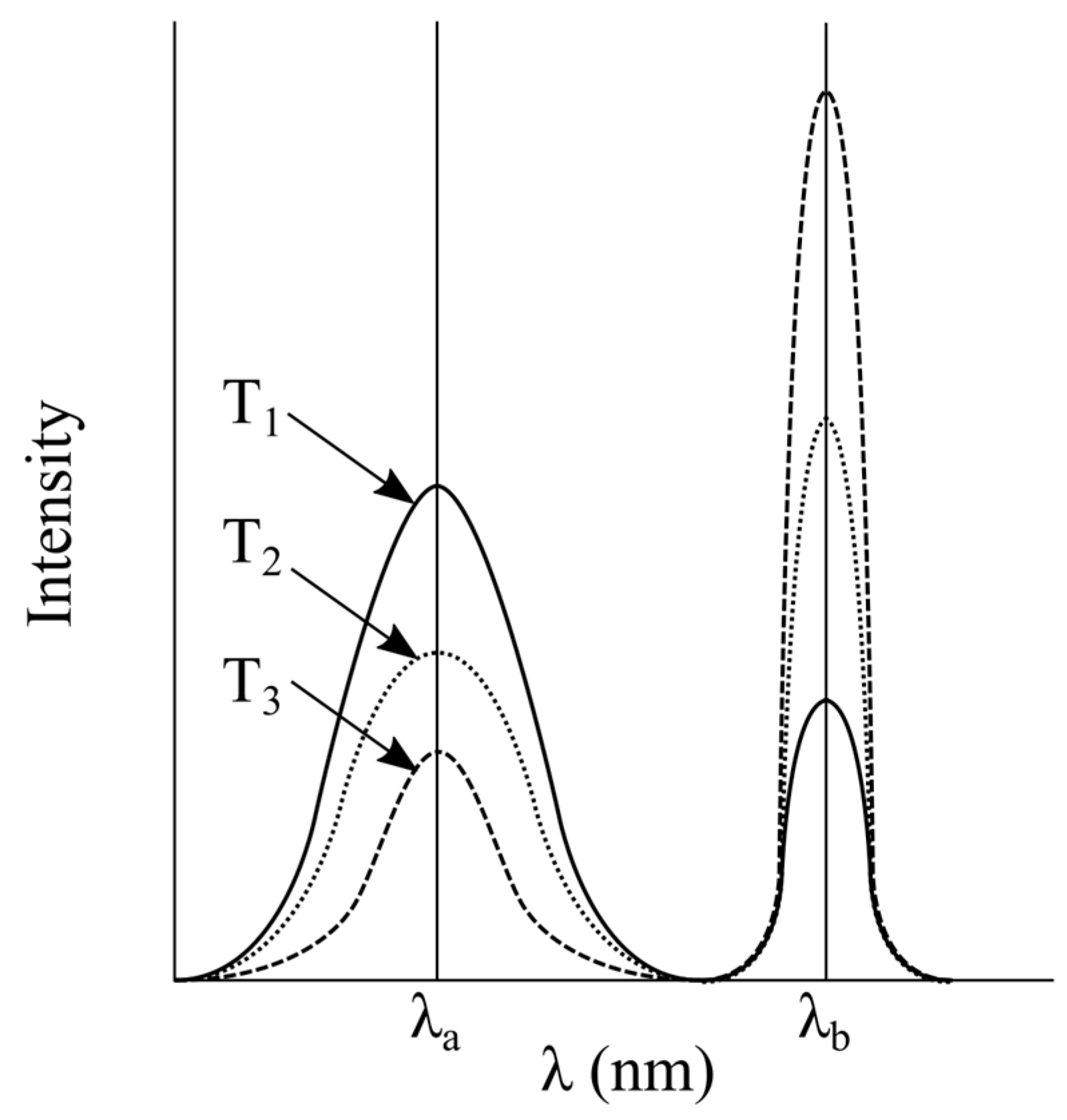
In photoluminescence thermometry, only excitation photons impinge on the sample. No physical or mechanical contact needs to be made between the thermometer and the emitting surface of the sample whose temperature is being measured. Moreover, temperature mapping of a small sample (biological, chemical, electrical, mechanical) is limited in spatial resolution only by the diameter of the excitation laser beam. High thermal resolutions are readily achievable. Intensity-based ratiometric luminescence thermometry becomes possible when a sample emits light from bands centered at two different wavelengths, λa and λb, where the intensity ratio of the two bands Ia/Ib varies smoothly and monotonically with variations in the sample temperature [6,7,8]. The intensity ratio thermometer is calibrated by measuring Ia/Ib of a standard at a series of known temperatures. A plot of the experimentally determined R = Ia/Ib luminescence intensity ratio of the sample vs. temperature, expressed as a power series to give the fitting coefficients a, b, c, d …, yields the desired temperature
T = a + bR + cR2 + dR3 +...
A typical temperature vs. luminescence intensity ratio plot is shown in Figure 8.
It is quite straightforward to implement the ratiometric luminescence intensity temperature measurement technique using modestly priced commercial luminescence spectrophotometers to acquire the T vs. R data sets (see Figure 5). Alternatively, the luminescence lifetime τ, the luminescence rise time tr, or the luminescence quantum yield Φ of a sample can be employed to measure sample temperature (Equation (10a–c)) [9,10,11] (see Figure 9):
T = a + bτ + cτ2 + dτ3 + …
T = a + btr + ctr2 + dtr3 +…
T = a + b Φ + c Φ2 + d Φ3 +…
The coefficients in the power series in Equations (9) and (10a–c) are determined by least squares fits of the T vs. R, T vs. tr, or T vs. Φ data sets measured at known temperatures.
It should be noted that lifetime thermometry can be quite challenging as it depends on several parameters such as duration and intensity of the signal and rise time of the equipment. The interested reader is referred to the luminescence lifetime investigations by Demas [12,13,14].
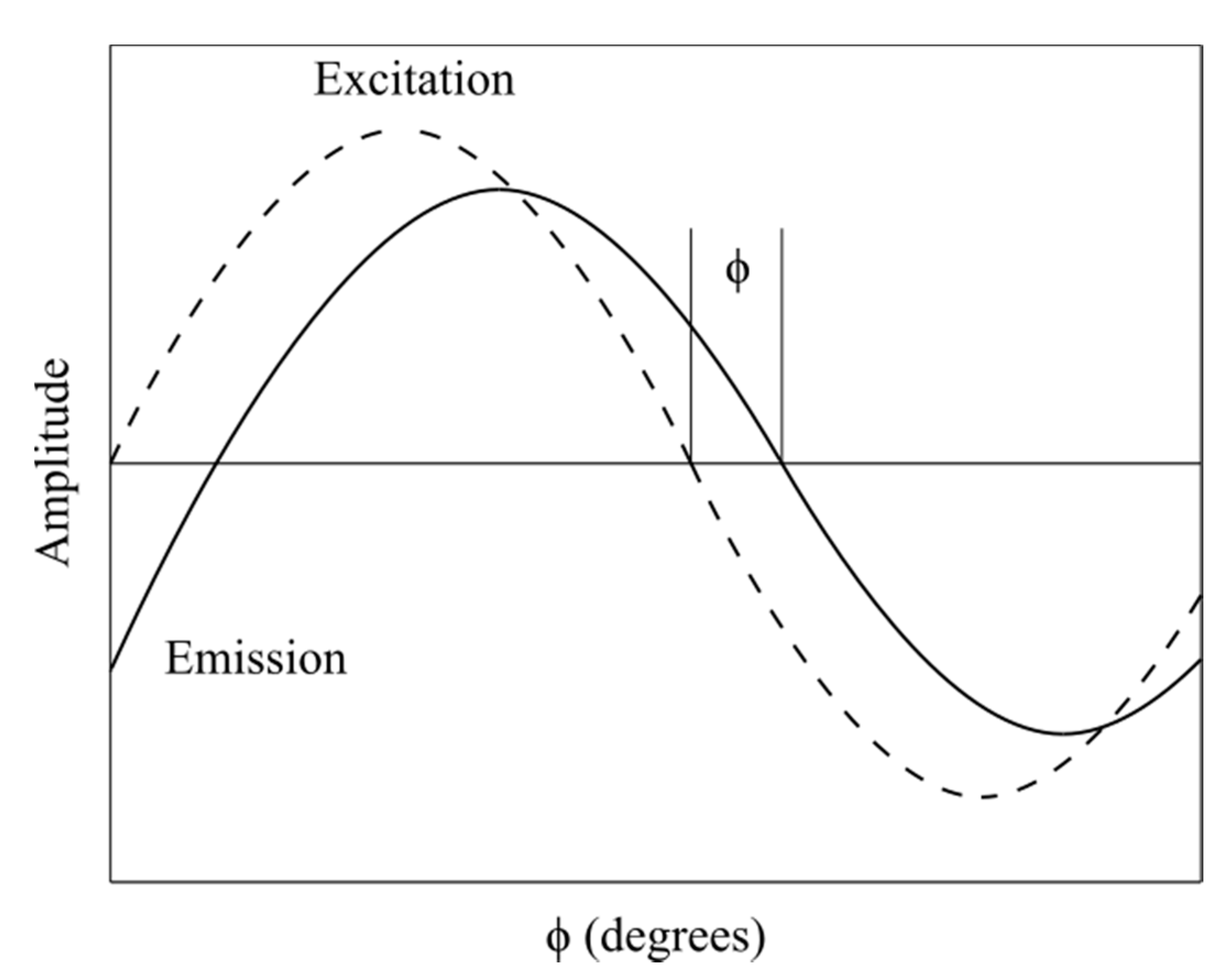
Luminescence lifetimes as a function of temperature can also be determined from the phase shift induced in the emitted light with respect to a sinusoidally modulated excitation source (Figure 10).
The experimentally determined lifetime τ is calculated from the expression (Equation (11)) relating the phase shift to the measured modulation frequency [15].
3.5. Temperature Scales for Thermometry
In 1989, the International Temperature Scale (ITS-90) [16] was adopted by the International Committee for Weights and Measures (CPIM). This temperature scale, based upon 16 fixed or defining points, spans the range from 0.65 K to the highest temperatures that can be measured by the Planck radiation law using monochromatic light. Almost all luminescence thermometry measurements and systems use ITS-90 directly or indirectly for calibration. For temperatures in the 0.9 mK to 1 K range, the Provisional Low Temperature Scale (PLTS-2000) is used [17]. A new temperature scale based upon 3He vapor pressure was adopted in 2006 (PTB-2006) [18]. This temperature scale transitions into PLTS-2000 below 1 K and into ITS-90 above 2 K. These temperature scales approximate the thermodynamic temperature scale and serve to define the international Kelvin and Celsius temperatures. The ITS-90 delivers temperatures determined by primary standard thermometry to 16 highly reproducible states of matter (e.g., triple point of water, melting point of gallium, and freezing point of copper). The PLTS-2000 scale employs the melting pressure of 3He for measuring temperature. These scales are used either directly or indirectly for all calibrations associated with luminescence thermometry.
4. Luminescence Temperature Measurement: Emissive Materials and Systems
4.1. Oxides of Lanthanide Metals
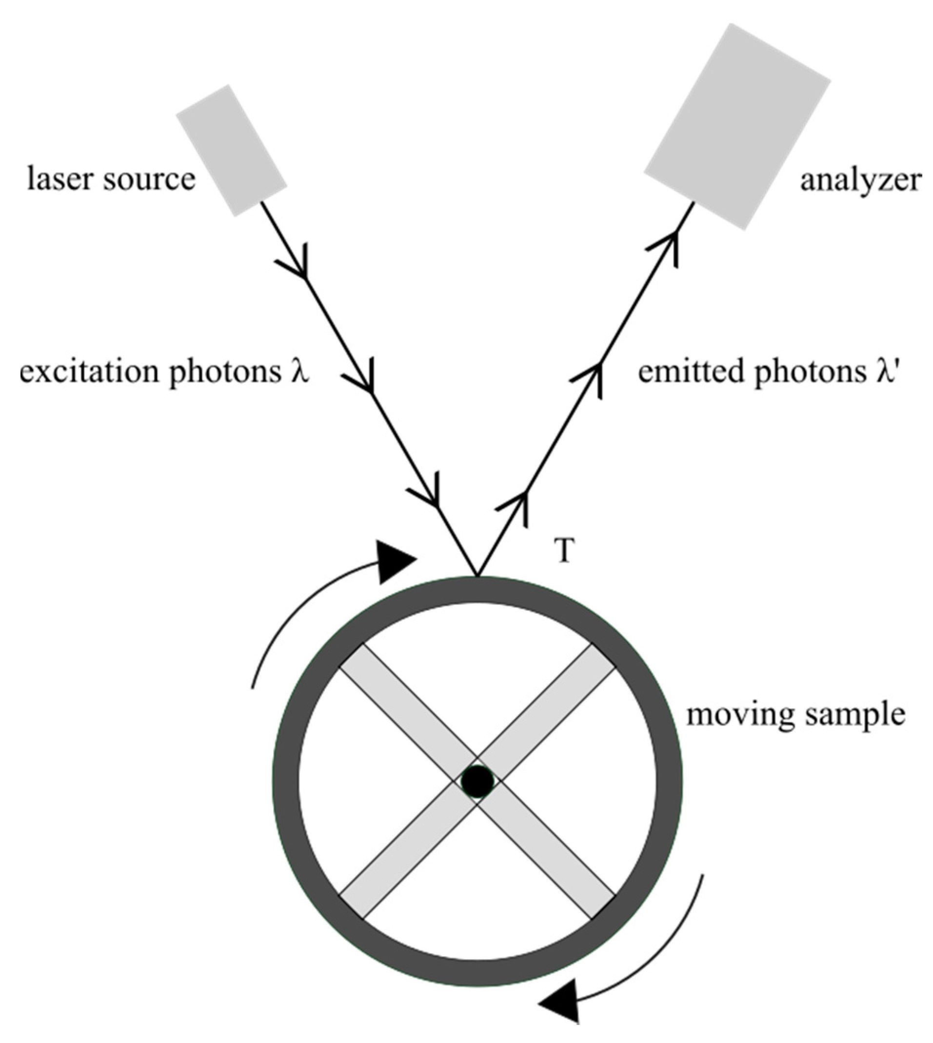
Aggressive environments such as corrosives, strong acids and bases, radioactive nuclides, flames, and rapidly moving high temperature devices and components (e.g., turbine blades in jet aircraft engines, moving parts in piston-driven internal combustion engines, and rocket engine nozzles) pose special thermometric challenges. Sensor-sample mechanical contact thermometry simply does not work for measuring the temperatures of hot jet engine turbine blades spinning at ~10,000 rpm at ~1000 K. An alternative non-contact temperature measurement approach is to exploit the temperature dependence of luminescent lanthanide metal oxide systems to measure temperature in these extreme environments [19]. Since lanthanide metal oxide coatings are used to protect the hot turbine blades, they are already physically present and available as chromophores for laser-induced temperature-dependent photoluminescence measurements (Figure 11).
This complements the increasing use of lanthanide-oxide films as barrier coatings in jet engines and other rapidly moving high temperature systems. Non-contact thermometry under these extreme conditions is straightforwardly implemented by laser excitation of the moving parts followed by measurement of the luminescence spectral profile for ratiometric studies and/or luminescence lifetime τ or rise time tr of the lanthanide-oxide chromophore [19].
4.2. Temperature Sensing Luminescence Chromophores I: Organic and Metal Organic Materials
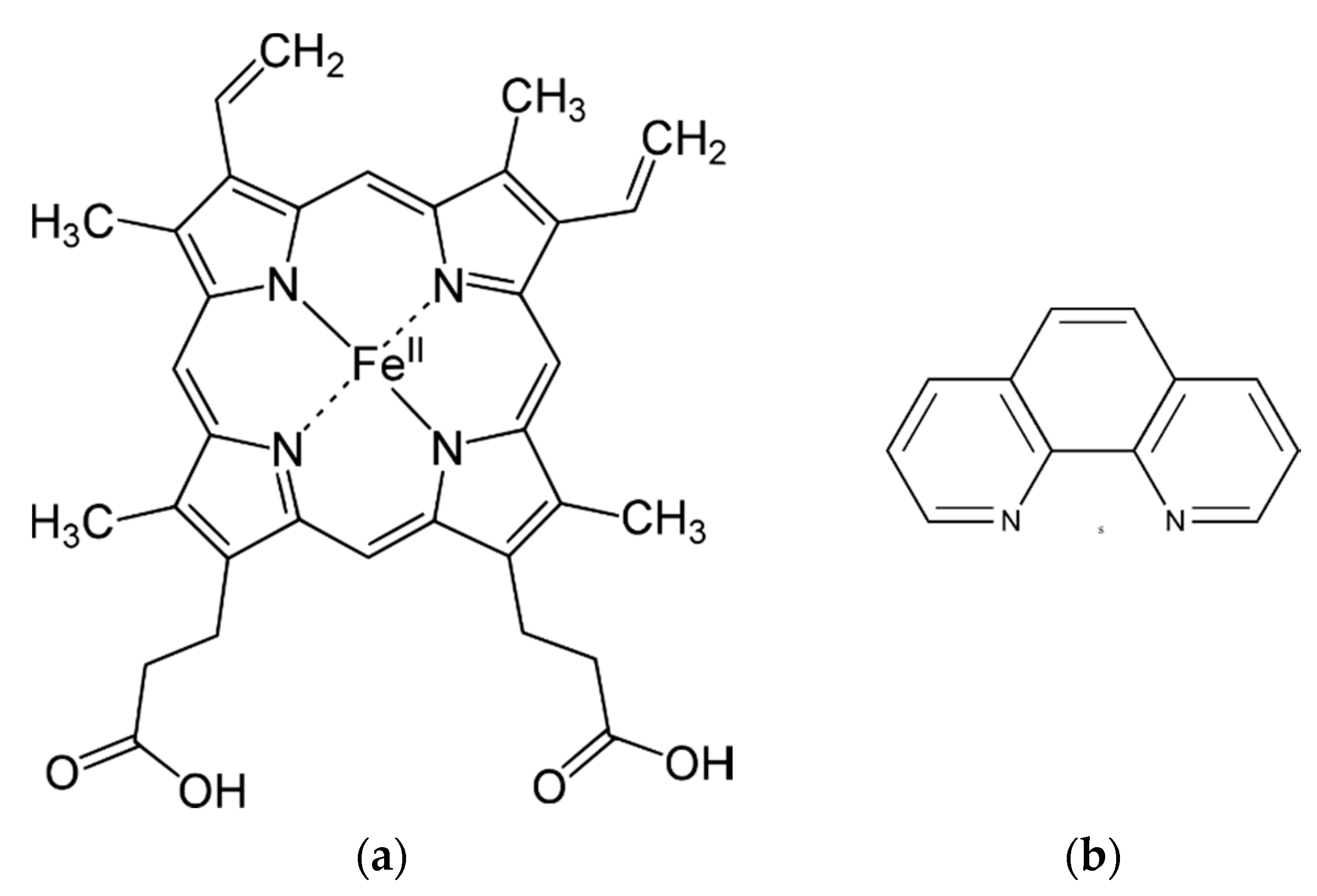
The luminescence lifetimes and luminescence intensities of many organic and metal organic molecules—particularly organic molecules with extended conjugated π orbital systems (see Figure 12)—are sensitive functions of temperature [20,21,22,23].
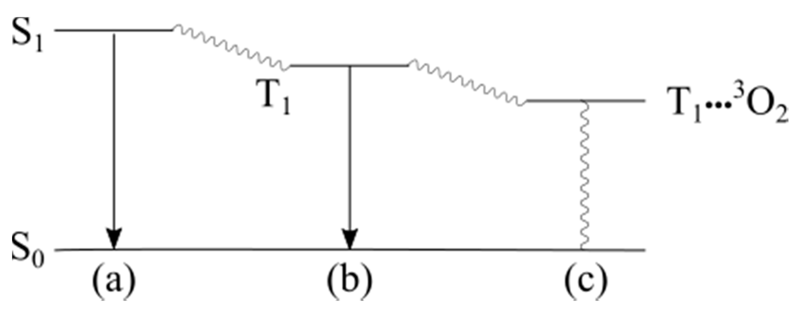
A typical organic chromophore has a singlet electronic ground state S0 with all electron spins paired, singlet lowest energy excited state S1 also with all electron spins paired, and a lowest energy triplet excited state T1 with two unpaired electron spins [20]. If these organic molecules are soluble in water and/or other solvents, they are called dyes. If the molecules are not water or solvent soluble, they are called pigments. Dye/pigment molecules absorb and are excited by selected wavelengths of near-UV, visible, and near-IR light giving their characteristic brilliant colors. Many but by no means all of these dye–pigment molecules also emit light in the visible and near-IR. Luminescent dyes and pigments tend to have more rigid structures that inhibit the non-radiative dissipation of energy of the excited molecule via molecular vibrations. Excited state energy deposited in the molecule by the excitation light is dissipated radiatively via a visible or near-IR photon. In contrast, non-emitting molecules tend to be more fluxional allowing non-radiative dissipation of the excited state energy to occur via molecular vibrations in the mid-to-far infrared. Increasing temperature favors non-radiative energy dissipation pathways. Luminescence intensity is diminished, and luminescence lifetime and quantum yield are also diminished. In this case, luminescence is said to be partially quenched. A totally quenched dye/pigment is non-luminescent. Luminescence from a typical dye/pigment is induced by excitation light and partially or completely quenched by triplet oxygen as shown in the Jablonski diagram in Figure 13 [24].
4.3. Temperature Sensing Luminescence Chromophores II: Transition Metal Complexes
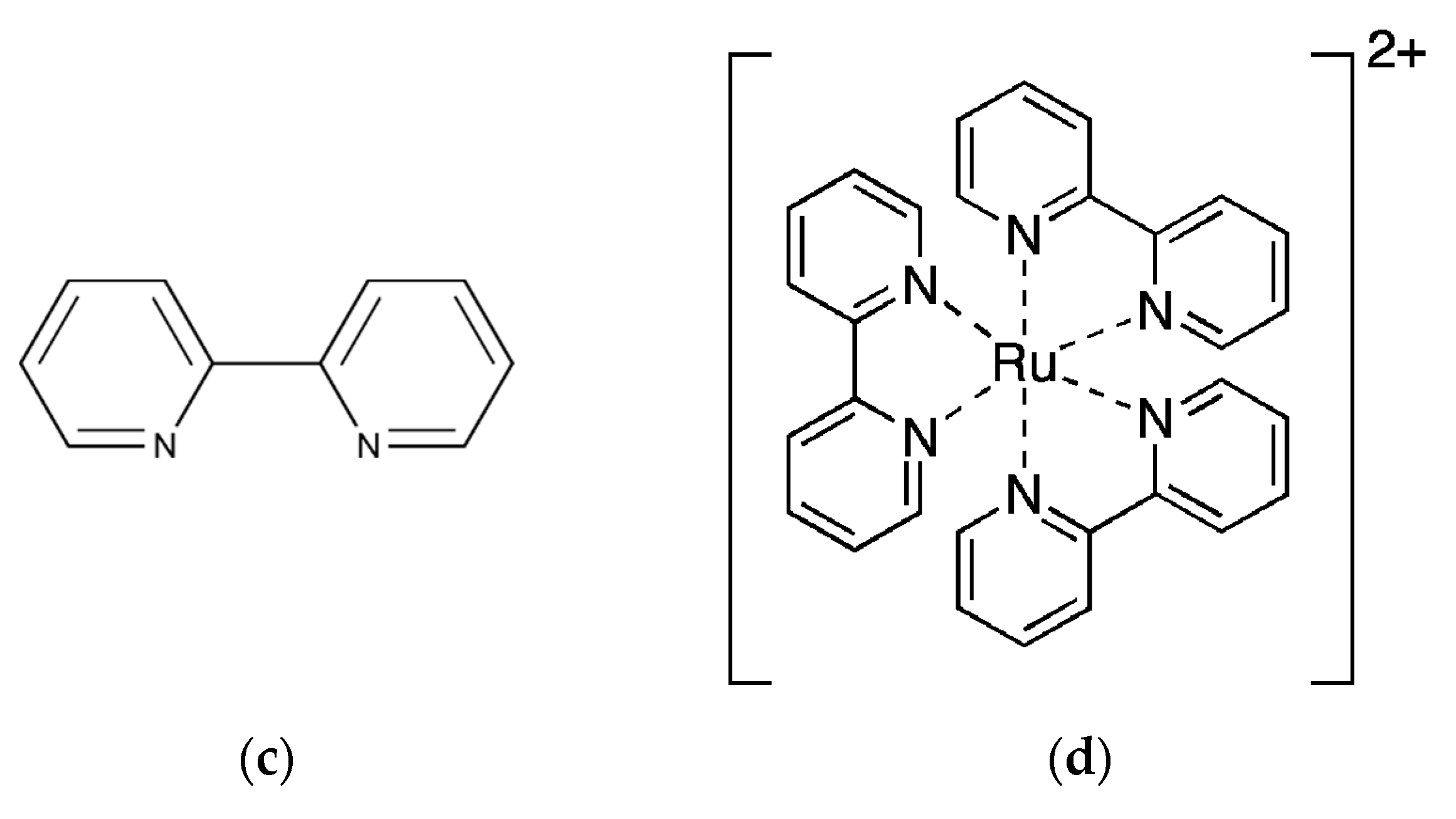
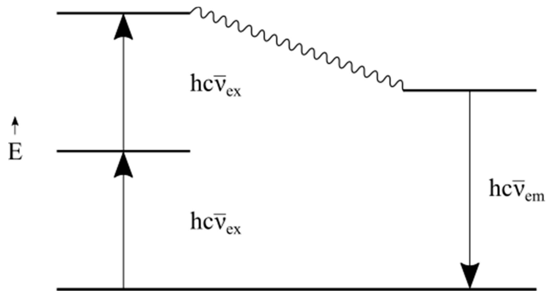
Transition metal complexes, especially those whose ligands are comprised of polycyclic aromatic π conjugated systems, exhibit significant temperature-dependent luminescence intensity and luminescence lifetime behavior over a wide range of temperatures [20,21]. For example, the chromophore [Ru(bpy)3]2+ where the ligand 2,2′-bipyridine, abbreviated bpy, can support luminescence-based thermometry via temperature-dependent luminescence lifetimes and intensities in the 50–290 K range, as shown in Figure 14.
The bpy ligand is bidentate. It is comprised of two pyridine rings, each with a nitrogen ligating atom joined by a single bond, around which rotational distortions can take place. The related chromophore [Ru(phen)3]2+ can support luminescence-based thermometry at higher temperatures, 273–393 K, via temperature-dependent luminescence lifetimes and intensities. The bidentate ligand phen = 1,10-phenanthroline is much more rigid structurally than bpy. This allows for effective luminescence-based thermometry in phen transition metal complexes at significantly higher temperatures than what is achievable with bpy complexes. Many complexes of ruthenium, platinum, iridium, and other metals with multidentate aromatic ligands can serve as temperature sensors via fluorescence and phosphorescence emissions. Luminescence behavior in transition metal complexes that can, in principle, serve as temperature sensors may be metal centered (MC), ligand centered (LC), ligand-to-ligand charge transfer (LLCT), ligand-to-metal-charge-transfer (LMCT), or metal to-ligand-charge-transfer (MLCT) [25,26].
4.4. Temperature Sensing Luminescence Chromophores III: Transition Metal and Lanthanide Oxides
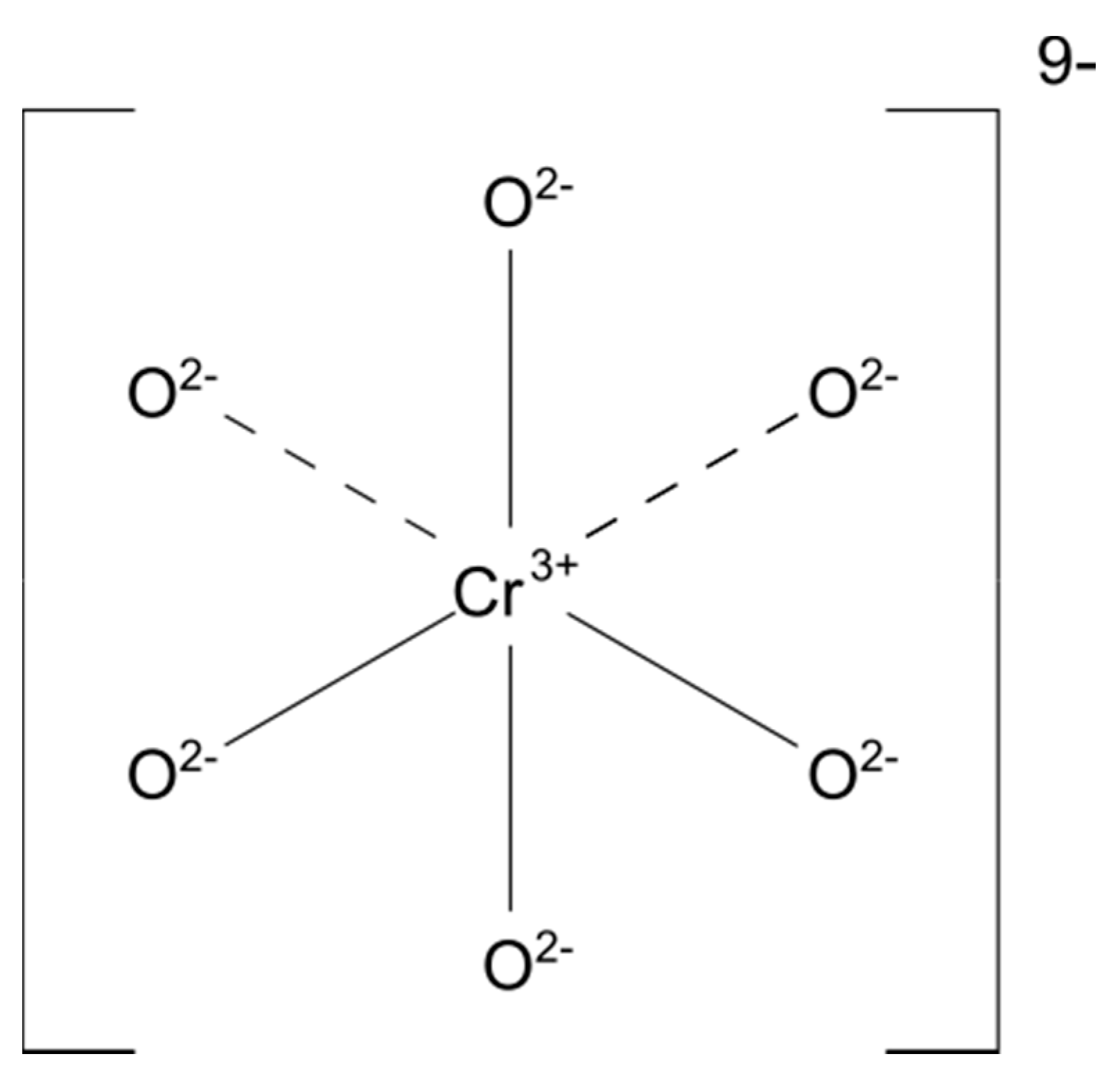
Luminescent metal ions doped in small concentrations into insulating and wide band-gap inorganic materials are extensively used as temperature and pressure sensors. The prototypical example of this type of system is ruby: aluminum oxide, Al2O3, into which a small percentage of lattice Al3+ cations is replaced by dopant Cr3+ cations [27]. The site geometry of the Cr3+ cations in aluminum oxide is distorted octahedral; each Cr3+ cation is surrounded by six nearest neighbor O2− anionic “ligands” [27]. Some exchange-coupled Cr3+–O2−–Cr3+ double metal sites in which two Cr3+ cations are adjacent, and are thus able to interact or couple electronically, may also occur in ruby. When doped into an insulator or wide band-gap inorganic material, the transition metal appears in the host as a cation with charge
+z = +1, +2, +3, +4, +5, or +6
First row transition metal cations with 3d valence orbitals exhibit many valence electron configurations of the type
where n = 1 to 10 is the number of valence electrons in the 3d orbitals of the transition metal cation symmetry. Partially filled 3d orbitals in transition metal cations give rise to a plethora of electronic energy states from which luminesce capable of supporting luminescence-based thermometry can occur. Tanabe–Sugano diagrams (Figure 15) provide excellent pictures of the disposition of the electronic states arising from [core](3d)n electron configurations [28,29].
[core](3d)n
The familiar 2Eg → 4A2g phosphorescence in ruby is a notable case in point. Third row transition metal cations in octahedral environments with the same number of 3d electrons tend to exhibit similar luminescence behaviors as exemplified by a comparison of the luminescence spectra of the [core] (3d)3 cations Mn4+ and Cr3+. The lanthanide metal cations have proven to be an excellent class of luminescence thermometers [22,30]. The most common oxidation states of these elements are +2 or +3, with the +3 oxidation state being more extensively utilized for luminescence thermometry. Like the 3d transition metal cations, cations of the 4f lanthanide elements yield multiple electron configurations and states that support temperature-dependent luminescence behavior as presented in a Dieke diagram [31,32,33]. Electronic states and transitions associated with the +3 lanthanide cations of a given element are quite different those corresponding states and transitions associated with the +2 cations of that same element. In the +3 lanthanide cations, all valence d and s electrons are removed. The valence electron configuration of a lanthanide cation Ln3+ is [core](4f)n where the number of valence 4f electrons is n = 1 to 13. Electronic transitions between the f-f states of Ln3+ cations are orbitally forbidden (Laporte rule) formally but become allowed with a reduction in symmetry of the local environment. The f-f luminescence transitions of different Ln3+ cation guest/matrix host systems therefore reflect the individual Ln3+ guest/matrix host interactions. These interactions are temperature dependent and can be used for luminescence temperature sensors (see Figure 16).
Emissive fluoride-containing matrices into which lanthanides are dispersed represent an important class of luminescent materials potentially useful in luminescence thermometry. The luminescent material Er:Yb:NaY2F5O, for example, has been proven to function effectively for temperature measurements of biological tissues based upon luminescence upconversion [37]. However, care must be taken regarding their use. For example, in emissions from NaYF4:Eu3+ (5D1 and 5D0), where Eu3+ ions are present only in low concentrations, Boltzmann thermal equilibrium is not achieved in the 300–900 K range [38]. In the absence of Boltzmann thermal equilibration, the determination of temperature by luminescence intensity ratios becomes problematical. However, increasing the Eu3+ concentration increases the number of closely spaced Eu3+ ion pairs and thus facilitates 5D1–5D0 cross relaxation leading to the achievement of thermal equilibrium and extension of the viable temperature measurement range to the full 500 K−900+ K temperature window.
4.5. Temperature Sensing Luminescence Chromophores IV: Semiconductor Quantum Dots
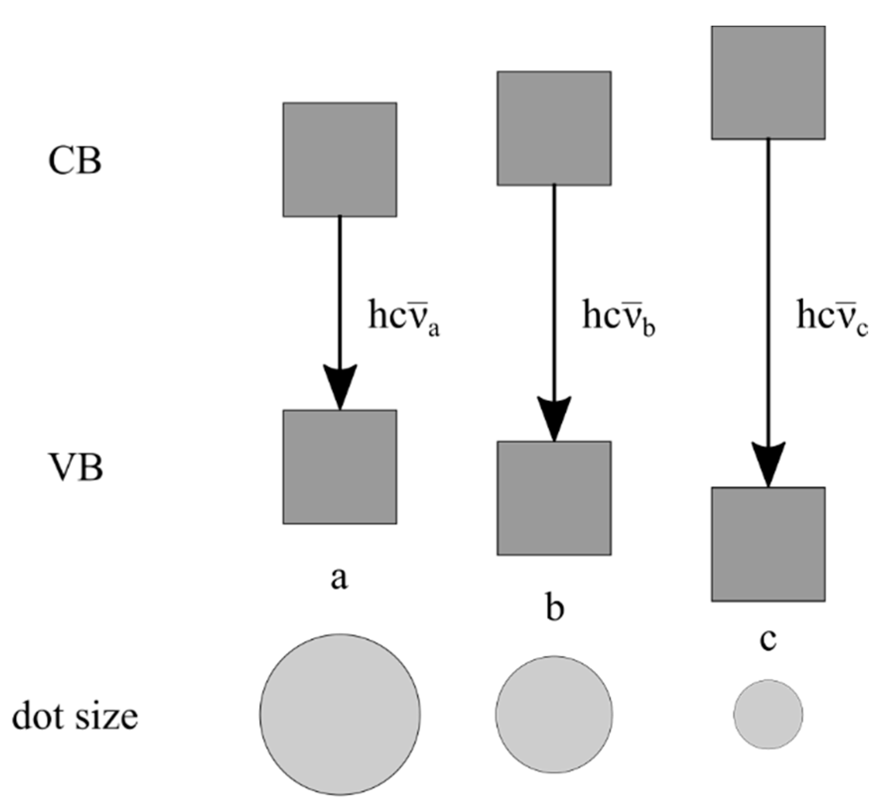
Quantum dots (QDs) are semiconductor systems intermediate in size between individual atoms and bulk solid state materials [39,40]. A typical QD is comprised of a few hundred to a few thousand atoms [41,42]. In contrast, consider a ~0.1 mg bulk sample of silicon, the smallest bulk amount that can be weighed on a standard laboratory analytical balance. This 0.1 mg sample is comprised of ~2 × 10¹⁸ silicon atoms! The small size of QDs leads to quantum confinement effects similar in many aspects to the familiar particle-in-a-box quantum systems (Figure 17). These quantum effects are quite different from the quantum effects observed in single atoms and bulk materials. In QD systems, it is common to see properties that are a combination of atomic and bulk material properties. QDs exhibit large size-dependent changes in optical properties including high luminescence intensity and high thermal sensitivity of luminescence, making them excellent candidates for luminescence-based thermometry [43].
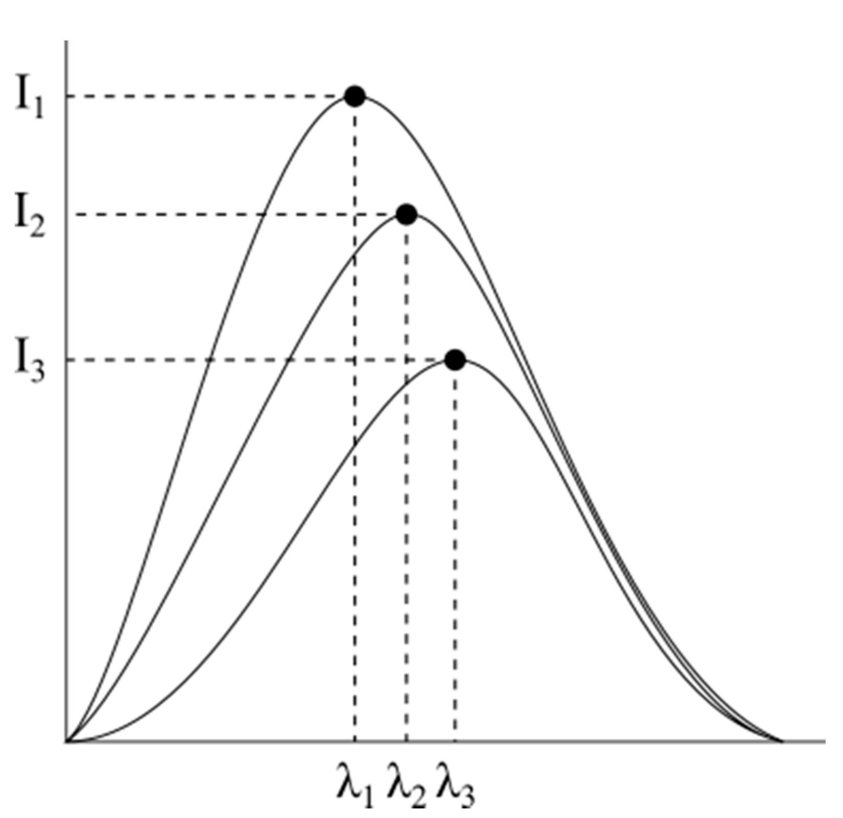
QD luminescence is also pressure dependent; dual mode temperature-pressure measurements are a possible application of QD systems [44]. The small size of QDs (nanometers) makes them excellent temperature nanosensors. Overall, temperature sensitivity of QDs (e.g., lead sulfide, PbS) increases with QD size and approaches the bulk values (~500 μeVK−1) in the large QD size limit (~15.5 nm). QD luminescence can be used for intracellular temperature mapping in biology and microelectronic circuit temperature mapping in semiconductor electronics industries. QDs provide excellent, reproducible temperature-dependent changes in luminescence wavelength maxima, spectral bandwidths, intensities (see Figure 18), and lifetimes that can be exploited for temperature measurement. Luminescence band profiles of QD systems are Gaussian [45,46].
Peak energies of these QD luminescence bands depend upon their composition, size, and the local microscopic environment into which they are imbedded. Temperature sensitivity of the band gap dEg/dT, and hence the energy and wavelength of the emitted photon, depend upon QD size. Luminescent QDs deposited on a moving part or component of a system (Figure 11) can provide a robust, sensitive, non-contact way to remotely monitor the system’s temperature and to map out temperatures differences in different parts of the system with nanometer resolution.
However, one important consideration with quantum dots is their easily changeable optical properties due to their dimensions in the nanometer range. For example, Cd/Te QDs, one of the most frequently used variants, has been noted to experience significant thermal expansion and increase in diameter once it reaches a critical temperature [47]. The expansion creates an additional red-shift in luminescence, interfering with the spectral shift used for luminescence thermometry by shifting the emission peak position. This problem can be circumvented with the use of proper surface coatings on the QDs. These are often organic ligand compounds that bind to the surface atoms of the QD and maintain its size in high temperatures. For example, the emission peak position remains constant at temperatures above 65 °C for Cd/Te QDs with a coating of per-6-thio-β-cyclodextrin, while the same QDs without surface coatings find their peak position shifting at the same temperature [47].
The tunability of the QDs in their luminescence characteristics via surface coating choice is thus one of the great advantages of using QDs as non-contact luminescence thermometers. Yet, the challenges of synthesizing and applying proper coatings on QDs is compounded by the extremely high sensitivity of QDs to their environments and nature and quality of solvents. For example, QDs produced with the same techniques often yield significantly different quantum yields [48]. Thus, for QD systems to reach their full potential, a better understanding of the effects of surface coatings on QDs is needed through advancements in nanotechnology.
5. Combined Simultaneous Temperature and Property Measurements via Luminescence
In principle, luminescence can be employed to measure temperature and other properties of the system such as pressure, pH, dissolved oxygen concentration, and electric and magnetic field strength. Examples of some dual property measurement systems are discussed in the following subsections.
5.1. Temperature and Modest Pressure: Temperature- and Pressure-Dependent Luminescent Paints
The luminescence properties of platinum(II) porphyrin complexes Pt(porph) and ruthenium(II) tris-imine complexes such as [Ru(bpy)3]2+ and [Ru(phen)3]2+ where bpy = 2,2′-bipyridine and phen = 1,10-phenanthroline are used to measure the pressures on airfoils and surfaces in wind tunnels [49]. These complexes are dispersed in oxygen-permeable and therefore pressure sensitive paints or coatings that can be applied to the aerodynamic surfaces under test [50]. Greater air pressure at a given point on an airfoil results in greater oxygen concentration of the oxygen-permeable membrane into which the ruthenium chromophore is imbedded and increased quenching of the luminescence of the chromophore resulting in a lower pressure-dependent luminescence intensity. Designs for dual luminescence sensors comprised of two emitting species that luminesce in different spectral regions—one that is pressure sensitive and one that is temperature sensitive—are now available [51,52]. For example, consider a dual pressure-temperature measurement system that utilizes [Ru(phen)3]2+, whose luminescence is temperature dependent, and fullerene C70, whose luminescence is pressure dependent but insensitive to temperature. Temperature and oxygen concentration/pressure of this dual emission system are extracted from the luminescence lifetime [53].
5.2. Temperature and High Pressure Measurements in Diamond Anvil Cells
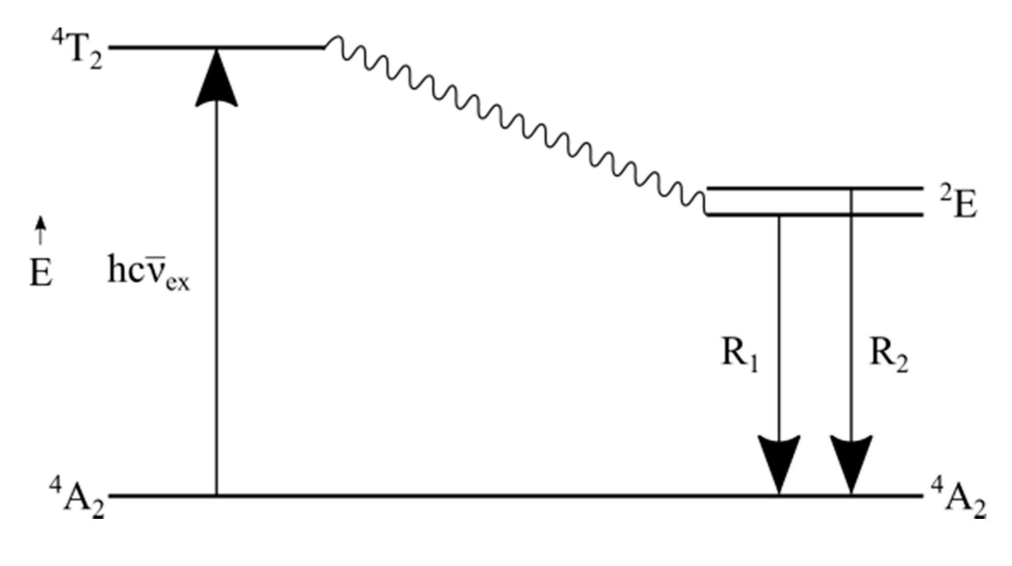
Diamond anvil cells provide a simple, compact, robust, and spectroscopically viable way to investigate the luminescence behaviors of substances at extreme pressures (~15 GPa) and at cryogenic temperatures (~10 K) [27]. As noted earlier, ruby—a form of doped aluminum oxide in which a small percentage of Al3+ cations in the lattice is replaced by Cr3+ cations—is well suited to serve as a pressure gauge and as a temperature gauge in diamond anvil cells via pressure- or temperature-induced spectral shifts in the sharp phosphorescence bands arising from the 2Eg → 4A1g phosphorescence transitions of the octahedrally coordinated Cr3+ cations in the aluminum oxide matrix (Figure 19). The phosphorescent chromophore in ruby is [CrO6]9−, which can be thought of as a “complex” comprised of a central Cr3+ cation and six O2− ligands.
The sites occupied by the Cr3+ cations in the lattice are thus modestly distorted octahedral sites that split the 3d Cr3+ orbitals into two sets: a lower energy set labeled t2g comprised of the dxy, dxz, dyz orbitals and a higher energy set labeled eg comprised of the dz2 and dx2–y2 orbitals. The lowest energy orbital configuration is [core](t2g)3 from which the 4A2g ground state of this system arises with a (dxy)α(dxz)α(dyz)α quartet spin arrangement. The lowest excited state is the 2Eg spin flip state, which also arises from the [core](t2g)3 electron configuration with a doublet (dxy)α(dxz)β(dyz)αspin arrangement where α = up spin and β = down spin. Referring to the lower energy states of the d3 Tanabe–Sugano Diagram (Figure 15), it is apparent that the energy of the 2Eg state exhibits a modest decrease with respect to increasing pressure, thus decreasing the energy of the 2Eg → 4A1g phosphorescence transitions and introducing measurable spectral red redshifts that can be used to measure pressure and temperature. Moreover, this decrease in phosphorescence energy with increasing pressure holds for both the R1 and R2 components of the 2Eg excited state (Figure 20) [54].
5.3. Luminescence-Based Measurements of Electric Fields
Application of an electric field E to a luminescent sample may induce observable changes in the luminescence from the sample arising from splittings or shifts in the wavelength, intensity, spectral bandwidth, or polarization of a luminescence band or bands. This is called the Stark Effect. Stark effects can be linear (effect proportional to E = E1) or quadratic (effect proportional to E2). With suitable calibration, a sample manifesting these Stark Effect emission phenomena may be used as a sensor to measure the strength and orientation of an applied electric field. Dual luminescence-electric field sensors are possible in which one sensor is sensitive to temperature and insensitive to electric field and the other sensor is insensitive to temperature and sensitive to electric field [55].
5.4. Luminescence-Based Measurements of Magnetic Fields
Readily observable perturbations frequently appear in the luminescence spectra of substances subjected to magnetic fields. A magnetic field B acts to split and shift the quantum energy levels and the luminescence bands emanating from transitions between these magnetically perturbed energy levels. Emission band intensities and lifetimes are also affected by magnetic fields. This magnetic-field-dependent splitting of quantum energy levels is termed the Zeeman Effect. Selected organic films and organic semiconductors such as tetracene and rubricene exhibit singlet exciton fission, a phenomenon known to be dependent on the magnitude and direction of the applied magnetic field. Rubricene, for example, forms amorphous films that exhibit large perturbations in their photoluminescence behavior when subjected to an applied magnetic field. These effects can be exploited to produce high resolution luminescence-based microscopic magnetic field maps [56].
6. Luminescence-Based Temperature Measurements in Molecular Biology and Biomedicine
While the luminescence thermometry technique is now well established in diverse areas of science and technology, the main roadblock to its widespread usage in the biomedical field arises from the complicated optical properties of human tissues. Tissue luminescence arises from the summative contributions of emitted light from vitamins, aromatic amino acids, proteins, and porphyrins. The human skin is composed of a variety of different chemicals and layers, each with different absorption and scattering properties, which severely hamper the extent to which visible and UV light can penetrate. Therefore, the excitation light must be restricted to specific wavelength ranges to ensure it can reach organs and deeper tissues of interest. Even after bypassing the issue of optical skin barriers, many more factors must be fulfilled for biomedical use of luminescence thermometry for temperature measurement to be viable. For example, the luminescent dopant particles that give rise to emission must be nontoxic and enter and exit the body noninvasively at the desired rates.
Recent studies have established this specific wavelength range to be in the infrared, with most of the wavelength range above 1000 nm. These ranges are termed “biological windows.” Three principal ranges have been designated: Region I, 750–950 nm; Region II, 1000–1350 nm; Region III, 1550–1870 nm [57]. Only the first and second biological windows are in widespread use for medical and biological purposes at the clinical level at this time (e.g., bioimaging and biothermometry), while current research is focused on the exploitation of the third long-wavelength infrared biological window that can further minimize loss of emitted light intensity by absorption into and scattering from the tissues. Penetration of higher energy UV and visible excitation photons into tissues is dramatically inhibited by Rayleigh scattering. Penetration intensity drops off with the 4th power of the wavelength (~1/λ4) [58]. Thus, longer wavelength infrared excitation light is strongly preferred over visible light if deep penetration of the excitation radiation into the tissues is needed.
Currently, the technique that best satisfies all these requirements and has potential temperature resolution of ±0.1°C is based upon the luminescence upconversion spectroscopy of emissive water-dispersed lanthanide nanoparticles (e.g., NaYF4:Er3+,Yb3+) doped into individual cells and the intercellular region. Luminescence upconversion spectroscopy [59] is capable of monitoring temperatures in individual biological cells as well as the intercellular region. For example, two infrared excitation photons, each with energy can induce a luminescence that is higher in energy than the individual hn excitation photons. This is in contrast to traditional Stokes shift in classical luminescence spectroscopy, where the emission photon energy is lower than the excitation photon energy [60]. While upconversion happens in various ways, the most basic explanation is the combination of multiple low-energy photons yield one higher-energy excitation photon. A two-photon luminescence upconversion process is shown, in Figure 21.
As shown in Figure 21, an upconverting nanoparticle is composed of two distinct elements: the sensitizer/absorber ion surrounding the emitter ion in a crystal lattice. When two photons from the sensitizer ion are transferred to the emitter ion, the two undergo a process of annihilation where one photon drops to ground state while the other photon gains all the energy and is promoted to a higher state. Thus, by producing one high-energy photon from two low-energy photons, the particle achieves upconversion and obeys conservation of energy [60].
One specific advantage of upconversion luminescence spectroscopy in biological systems as compared to traditional Stokes luminescence, lies in the suppression of autofluorescence. Autofluorescence typically occurs when the emitting chromophore luminesces naturally with a Stokes Shift, yielding emitted photons that are lower in energy than single excitation photons. Thus, autofluorescence rarely occurs with upconversion emission, as the individual excitation photons are too low in energy induce Stokes luminescence, improving both the thermal and spatial resolution [61].
A second advantage of upconversion is that due to this aforementioned structure, the luminescence only occurs when the emitter ion is surrounded by sensitizer ions. Thus, changes in the environment do not affect the emission, allowing the upconversion absorber/emitter species to maintain the same behavior in various biological fluids. Among the most promising materials for luminescence upconversion nanothermometers are lanthanide-doped nanoparticles (e.g., NaYF4:Er3+,Yb3+) [62].
7. Perspective
Luminescence-based thermometry, while not without challenges, provides an amazing diversity of viable techniques and materials that can be used for the measurement of temperature. Moreover, luminescence sensor technology can be deployed in such a way that it enables the simultaneous measurement of temperature and other quantities of interest: electric fields, magnetic fields, pressure, fluid flow, thermal profiles of electronic circuits and devices, numerous biomedical applications including intracellular and intercellular temperature measurements, and temperature mapping of microfluidic and nanofluidic systems. Advances in modern laser technology, laser spectroscopy, and material science are driving the emergence of new luminescence-based devices and thermometric techniques. Particularly noteworthy is the deployment of luminescence upconversion spectroscopy in biomedical applications to measure temperature and other properties in deep tissues and individual cells with nanoscale resolution. The wide range of luminescent materials that can be used as luminescence temperature and property sensors encourages experimentation and facilitates the development of sensors with specialized properties. While traditional contact thermometry enjoys the advantages of simplicity, accuracy, and modest cost, it cannot measure the temperatures of objects in motion. If the object whose temperature is to be measured is moving, non-contact luminescence thermometry shines. Luminescence sensors in the future could benefit from the implementation of more standardization and calibration protocols.
8. Conclusions
While traditional methods of thermometry have been and will continue to be important, new frontiers in science, engineering, and medicine will require ever more precise, sensitive, high resolution, contact, and non-contact thermometric methods. Luminescence thermometry is the perfect tool to accomplish this. Luminescence thermometry functions by exploiting various relationships between temperature and quantities that characterize luminescence, including spectral band maxima, bandwidths, intensity ratios, risetimes, and lifetime decay profiles. The four most commonly viable materials as sensors are lanthanide and transition metal doped systems, organic chromophores, and quantum dots. The unique physical properties of each of these materials create different niche temperature ranges and environmental conditions where each can function best. Future areas of study in thermometry should focus on developing new temperature scales compatible with the precise and narrow temperature ranges where luminescence thermometry is applicable. Studies should focus on the utilizing the potential of luminescence to also measure pressure, magnetic fields, and electric fields to create a single, multi-functional measurement tool. The scattering and absorption of UV-visible radiation by tissues poses a unique biomedical challenge and opportunity for luminescence thermometry. Further investigations into optimizing the upconversion spectroscopy can circumvent this problem and allow biomedicine to reap the full benefits of luminescence thermometry.
Author Contributions
Conceptualization, J.W.K.III and J.J.L.; formal analysis, J.W.K.III and J.J.L.; resources, J.W.K.III and J.J.L.; writing—original draft preparation, J.W.K.III and J.J.L.; writing—review and editing, J.W.K.III and J.J.L.; visualization, J.W.K.III and J.J.L.; project administration, J.W.K.III. All authors have read and agreed to the published version of the manuscript.
Funding
This research received no external funding.
Institutional Review Board Statement
Not applicable.
Informed Consent Statement
Not applicable.
Data Availability Statement
Not applicable.
Acknowledgments
The authors are pleased to acknowledge administrative support for the preparation of this manuscript from the Office of the Provost at Concordia University. The authors thank the referees for their careful reading of the manuscript and their valuable suggestions.
Conflicts of Interest
The authors declare no conflict of interest.
References
- Michalski, L.; Eckersdorf, K.; Kucharski, J.; McGhee, J. Temperature Measurement. Meas. Sci. Technol. 2002, 13, 1651–1652. [Google Scholar] [CrossRef]
- Infographic: Absolute Zero to ‘Absolute Hot’. Available online: https://www.bbc.com/future/article/20131218-absolute-zero-to-absolute-hot (accessed on 13 May 2021).
- Omega Engineering. Complete Temperature Measurement Handbook and Encyclopedia of Contents, 2nd ed.; Omega Engineering: Norwalk, CT, USA, 2000. [Google Scholar]
- Dramićanin, M. Luminescence Thermometry: Methods, Materials, and Applications. Lumin. Thermom. Methods Mater. Appl. 2018, 1–292. [Google Scholar] [CrossRef]
- Gianfrani, L. Linking the Thermodynamic Temperature to an Optical Frequency: Recent Advances in Doppler Broadening Thermometry. Philos. Trans. R. Soc. Math. Phys. Eng. Sci. 2016, 374, 20150047. [Google Scholar] [CrossRef] [PubMed] [Green Version]
- Nikolić, M.G.; Antić, Ž.; Ćulubrk, S.; Nedeljković, J.M.; Dramićanin, M.D. Temperature Sensing with Eu3+ Doped TiO2 Nanoparticles. Sens. Actuators B Chem. 2014, 201, 46–50. [Google Scholar] [CrossRef]
- Ćulubrk, S.; Lojpur, V.; Ahrenkiel, S.P.; Nedeljković, J.M.; Dramićanin, M.D. Non-Contact Thermometry with Dy3+ Doped Gd2Ti2O7 Nano-Powders. J. Lumin. 2016, 170, 395–400. [Google Scholar] [CrossRef]
- Dramićanin, M.D.; Antić, Ž.; Ćulubrk, S.; Ahrenkiel, S.P.; Nedeljković, J.M. Self-Referenced Luminescence Thermometry with Sm3+ Doped TiO2 Nanoparticles. Nanotechnology 2014, 25, 485501. [Google Scholar] [CrossRef] [PubMed]
- Marciniak, L.; Trejgis, K. Luminescence Lifetime Thermometry with Mn3+–Mn4+ Co-Doped Nanocrystals. J. Mater. Chem. C 2018, 6, 7092–7100. [Google Scholar] [CrossRef]
- Hager, G.D.; Crosby, G.A. Charge-transfer exited states of ruthenium (II) complexes. I. Quantum yield and decay measurements. J. Am. Chem. Soc. 1975, 97, 7031–7037. [Google Scholar] [CrossRef]
- Hager, G.D.; Crosby, G.A. Charge-transfer excited states of ruthenium (II) complexes. II. Relation of level parameters to molecular structure. J. Am. Chem. Soc. 1975, 97.24, 7037–7042. [Google Scholar] [CrossRef]
- Demas, J. Excited State Lifetime Measurements; Academic Press: New York, NY, USA, 1983; ISBN 978-012-208-920-6. [Google Scholar]
- Rowe, H.M.; Chan, S.P.; Demas, J.N.; DeGraff, B.A. Elimination of fluorescence and scattering backgrounds in luminescence lifetime measurements using gated-phase fluorometry. Anal. Chem. 2002, 74, 4821–4827. [Google Scholar] [CrossRef]
- Demas, J.N.; DeGraff, B.A., Jr. Design of luminescence-based temperature sensors. Chem. Biochem. Environ. Fiber Sens. IV 1993, 1796. [Google Scholar] [CrossRef]
- SPEX Fluorescence Group. Application Note F-10: Which Fluorescence Lifetime System Is Best For You? Available online: https://www.horiba.com/fileadmin/uploads/Scientific/Documents/Fluorescence/F-10.pdf (accessed on 13 May 2021).
- Preston-Thomas, H. The International Temperature Scale of 1990(ITS-90). Metrologia 1990, 27, 3–10. [Google Scholar] [CrossRef]
- Rusby, R.L.; Durieux, M.; Reesink, A.L.; Hudson, R.P.; Schuster, G.; Kühne, M.; Fogle, W.E.; Soulen, R.J.; Adams, E.D. The Provisional Low Temperature Scale from 0.9 MK to 1 K, PLTS-2000. J. Low Temp. Phys. 2002, 126, 633–642. [Google Scholar] [CrossRef]
- Engert, J.; Fellmuth, B.; Jousten, K. A New 3He Vapour-Pressure Based Temperature Scale from 0.65 K to 3.2 K Consistent with the PLTS-2000. Metrologia 2007, 44, 40–52. [Google Scholar] [CrossRef]
- Chambers, M.D.; Clarke, D.R. Doped Oxides for High-Temperature Luminescence and Lifetime Thermometry. Annu. Rev. Mater. Res. 2009, 39, 325–359. [Google Scholar] [CrossRef] [Green Version]
- Calvert, J.G.; Pitts, J.N., Jr. Photochemistry; John Wiley & Sons: New York, NY, USA, 1966; ISBN 978-047-113-090-1. [Google Scholar]
- Bustamante, N.; Ielasi, G.; Bedoya, M.; Orellana, G. Optimization of Temperature Sensing with Polymer-Embedded Luminescent Ru(II) Complexes. Polymers 2018, 10, 234. [Google Scholar] [CrossRef] [Green Version]
- Rocha, J.; Brites, C.D.; Carlos, L.D. Lanthanide Organic Framework Luminescent Thermometers. Chem. Eur. J. 2016, 22, 14782–14795. [Google Scholar] [CrossRef] [PubMed]
- Hipps, K.W.; Crosby, G.A. Charge-Transfer Excited States of Ruthenium(II) Complexes. III. Electron-Ion Coupling Model for dπ* Configurations. J. Am. Chem. Soc. 1975. [Google Scholar] [CrossRef]
- McGlynn, S.P.; Azumi, T.; Kinoshita, M. Molecular Spectroscopy of the Triplet State; Prentice-Hall International Series in Chemistry; Prentice Hall Press: Hoboken, NJ, USA, 1969. [Google Scholar]
- Allendorf, M.D.; Bauer, C.A.; Bhakta, R.K.; Houk, R.J.T. Luminescent Metal–Organic Frameworks. Chem. Soc. Rev. 2009, 38, 1330–1352. [Google Scholar] [CrossRef] [PubMed]
- Dorenbos, P. Charge Transfer Bands in Optical Materials and Related Defect Level Location. Opt. Mater. 2017, 69, 8–22. [Google Scholar] [CrossRef]
- Syassen, K. Ruby under Pressure. High Press. Res. 2008, 28, 75–126. [Google Scholar] [CrossRef]
- Tanabe, Y.; Sugano, S. On the Absorption Spectra of Complex Ions. I. J. Phys. Soc. Jpn. 1954, 9, 753–766. [Google Scholar] [CrossRef] [Green Version]
- Tanabe, Y.; Sugano, S. On the Absorption Spectra of Complex Ions II. J. Phys. Soc. Jpn. 1954, 9, 766–779. [Google Scholar] [CrossRef]
- Brites, C.D.; Balabhadra, S.; Carlos, L.D. Lanthanide-Based Thermometers: At the Cutting-Edge of Luminescence Thermometry. Adv. Optical. Mat. 2019, 7, 1801239. [Google Scholar] [CrossRef] [Green Version]
- Carnall, W.T.; Fields, P.R.; Rajnak, K. Spectral Intensities of the Trivalent Lanthanides and Actinides in Solution. II. Pm3+, Sm3+, Eu3+, Gd3+, Tb3+, Dy3+, and Ho3+. J. Chem. Phys. 1968, 49, 4412–4423. [Google Scholar] [CrossRef]
- Carnall, W.T.; Fields, P.R.; Rajnak, K. Electronic Energy Levels in the Trivalent Lanthanide Aquo Ions. I. Pr3+, Nd3+, Pm3+, Sm3+, Dy3+, Ho3+, Er3+, and Tm3+. J. Chem. Phys. 1968, 49, 4424–4442. [Google Scholar] [CrossRef]
- Dieke, G.H. Spectra and Energy Levels of Rare Earth Ions in Crystals; Crosswhite, H.M., Crosswhite, H., Eds.; Interscience Publishers: New York, NY, USA, 1968. [Google Scholar]
- Allison, S.W.; Beshears, D.L.; Cates, M.R.; Scudiere, M.B.; Shaw, D.W.; Ellis, A.D. Luminescence of YAG:Dy and YAG:Dy,Er Crystals to 1700 °C. Meas. Sci. Technol. 2020, 31, 044001. [Google Scholar] [CrossRef]
- Zhang, Z.Y.; Grattan, K.T.V.; Meggitt, B.T. Thulium-Doped Fiber Optic Decay-Time Temperature Sensors: Characterization of High Temperature Performance. Rev. Sci. Instrum. 2000, 71, 1614–1620. [Google Scholar] [CrossRef]
- Collins, S.F.; Baxter, G.W.; Wade, S.A.; Sun, T.; Grattan, K.T.V.; Zhang, Z.Y.; Palmer, A.W. Comparison of Fluorescence-Based Temperature Sensor Schemes: Theoretical Analysis and Experimental Validation. J. Appl. Phys. 1998, 84, 4649–4654. [Google Scholar] [CrossRef]
- Savchuk, O.A.; Haro-Gonzalez, P.; Carvajal, J.J.; Jaque, D.; Massons, J.; Aguilo, M.; Diaz, F. Er: Yb: NaY2 F5O up-Converting Nanoparticles for Sub-Tissue Fluorescence Lifetime Thermal Sensing. Nanoscale 2014, 6, 9727–9733. [Google Scholar] [CrossRef]
- Geitenbeek, R.G.; De Wijn, H.W.; Meijerink, A. Non-Boltzmann Luminescence in Na YF4: Eu3+: Implications for Luminescence Thermometry. Phys. Rev. Appl. 2018, 10, 064006. [Google Scholar] [CrossRef] [Green Version]
- Wang, Y.; Hu, A. Carbon Quantum Dots: Synthesis, Properties and Applications. J. Mater. Chem. C 2014, 2, 6921–6939. [Google Scholar] [CrossRef] [Green Version]
- Lim, S.Y.; Wei, S.; Zhiqiang, G. Carbon Quantum Dots and their Applications. Chem. Soc. Rev. 2015, 44, 362–381. [Google Scholar] [CrossRef]
- de Donegá, C.M. Synthesis and Properties of Colloidal Heteronanocrystals. Chem. Soc. Rev. 2011, 40, 1512–1546. [Google Scholar] [CrossRef] [PubMed] [Green Version]
- Xu, G.; Zeng, S.; Zhang, B.; Swihart, M.T.; Yong, K.-T.; Prasad, P.N. New Generation Cadmium-Free Quantum Dots for Biophotonics and Nanomedicine. Chem. Rev. 2016, 116, 12234–12327. [Google Scholar] [CrossRef]
- Walker, G.W.; Sundar, V.C.; Rudzinski, C.M.; Wun, A.W.; Bawendi, M.G.; Nocera, D.G. Quantum-Dot Optical Temperature Probes. Appl. Phys. Lett. 2003, 83, 3555–3557. [Google Scholar] [CrossRef]
- Phillips, J.; Bhattacharya, P.; Venkateswaran, U. Pressure-Induced Energy Level Crossings and Narrowing of Photoluminescence Linewidth in Self-Assembled InAlAs/AlGaAs Quantum Dots. Appl. Phys. Lett. 1999, 74, 1549–1551. [Google Scholar] [CrossRef] [Green Version]
- Chatten, A.J.; Barnham, K.W.J.; Buxton, B.F.; Ekins-Daukes, N.J.; Malik, M.A. A New Approach to Modelling Quantum Dot Concentrators. Sol. Energy Mater. Sol. Cells 2003, 75, 363–371. [Google Scholar] [CrossRef]
- Barnham, K.; Marques, L.J.; Hassard, J.; O’Brien, P. Quantum-Dot Concentrator and Thermodynamic Model for the Global Redshift. Appl. Phys. Lett. 2000, 76, 1197–1199. [Google Scholar] [CrossRef]
- Carlos, L.D.; Palacio, F. Thermometry at the Nanoscale: Techniques and Selected Applications; Royal Society of Chemistry: London, UK, 2015; ISBN 978-184-973-904-7. [Google Scholar]
- Silvi, S.; Credi, A. Luminescent Sensors Based on Quantum Dot–Molecule Conjugates. Chem. Soc. Rev. 2015, 44, 4275–4289. [Google Scholar] [CrossRef]
- Klein, C.; Engler, R.H.; Henne, U.; Sachs, W.E. Application of Pressure-Sensitive Paint for Determination of the Pressure Field and Calculation of the Forces and Moments of Models in a Wind Tunnel. Exp. Fluids 2005, 39, 475–483. [Google Scholar] [CrossRef]
- McLachlan, B.G.; Bell, J.H. Pressure-Sensitive Paint in Aerodynamic Testing. Exp. Therm. Fluid Sci. 1995, 10, 470–485. [Google Scholar] [CrossRef]
- Zelelow, B.; Khalil, G.E.; Phelan, G.; Carlson, B.; Gouterman, M.; Callis, J.B.; Dalton, L.R. Dual Luminophor Pressure Sensitive Paint: II. Lifetime Based Measurement of Pressure and Temperature. Sens. Actuators B Chem. 2003, 96, 304–314. [Google Scholar] [CrossRef]
- Stich, M.I.J.; Nagl, S.; Wolfbeis, O.S.; Henne, U.; Schaeferling, M. A Dual Luminescent Sensor Material for Simultaneous Imaging of Pressure and Temperature on Surfaces. Adv. Funct. Mater. 2008, 18, 1399–1406. [Google Scholar] [CrossRef]
- Borisov, S.M.; Vasylevska, A.S.; Krause, C.; Wolfbeis, O.S. Composite Luminescent Material for Dual Sensing of Oxygen and Temperature. Adv. Funct. Mater. 2006, 16, 1536–1542. [Google Scholar] [CrossRef]
- Kenney, J.W. Pressure Effects on Emissive Materials. In Optoelectronic Properties of Inorganic Compounds; Roundhill, D.M., Fackler, J.P., Eds.; Modern Inorganic Chemistry; Springer US: Boston, MA, USA, 1999; pp. 231–268. ISBN 978-1-4757-6101-6. [Google Scholar]
- Bublitz, G.U.; Boxer, S.G. STARK SPECTROSCOPY: Applications in Chemistry, Biology, and Materials Science. Annu. Rev. Phys. Chem. 1997, 48, 213–242. [Google Scholar] [CrossRef] [Green Version]
- Hodges, M.P.P.; Grell, M.; Morley, N.A.; Allwood, D.A. Wide Field Magnetic Luminescence Imaging. Adv. Funct. Mater. 2017, 27, 1–7. [Google Scholar] [CrossRef] [Green Version]
- Hemmer, E.; Benayas, A.; Légaré, F.; Vetrone, F. Exploiting the Biological Windows: Current Perspectives on Fluorescent Bioprobes Emitting above 1000 Nm. Nanoscale Horiz. 2016, 1, 168–184. [Google Scholar] [CrossRef]
- Jacques, S.L. Optical Properties of Biological Tissues: A Review. Phys. Med. Biol. 2013, 58, R37–R61. [Google Scholar] [CrossRef]
- Fischer, L.H.; Harms, G.S.; Wolfbeis, O.S. Upconverting Nanoparticles for Nanoscale Thermometry. Angew. Chem. Int. Ed. 2011, 50, 4546–4551. [Google Scholar] [CrossRef]
- Zijlmans, H.J.M.A.A.; Bonnet, J.; Burton, J.; Kardos, K.; Vail, T.; Niedbala, R.S.; Tanke, H.J. Detection of Cell and Tissue Surface Antigens Using Up-Converting Phosphors: A New Reporter Technology. Anal. Biochem. 1999, 267, 30–36. [Google Scholar] [CrossRef] [PubMed]
- Monici, M. Cell and tissue autofluorescence research and diagnostic applications. In Biotechnology Annual Review; Elsevier: Amsterdam, The Netherlands, 2005; Volume 11, pp. 227–256. [Google Scholar]
- Dong, H.; Du, S.-R.; Zheng, X.-Y.; Lyu, G.-M.; Sun, L.-D.; Li, L.-D.; Zhang, P.-Z.; Zhang, C.; Yan, C.-H. Lanthanide Nanoparticles: From Design toward Bioimaging and Therapy. Chem. Rev. 2015, 115, 10725–10815. [Google Scholar] [CrossRef] [PubMed]
Figure 1.
Liquid-in-glass thermometer at three different temperatures.

Figure 2.
Gas thermometer at three different temperatures.

Figure 3.
Type T thermocouple thermometer showing copper and copper-nickel (Constantan) reference and sample junctions.
Figure 3.
Type T thermocouple thermometer showing copper and copper-nickel (Constantan) reference and sample junctions.

Figure 4.
Resistance temperature device (RTD) showing calibrated resistor R and high impedance digital multimeter set to read ohms (Ω).
Figure 4.
Resistance temperature device (RTD) showing calibrated resistor R and high impedance digital multimeter set to read ohms (Ω).

Figure 5.
Plot of temperature T vs. thermocouple voltage V for a Type T copper–Constantan thermocouple with a water-ice reference junction. A polynomial least squares fit of the data yields the coefficients in the power series expansion.
Figure 5.
Plot of temperature T vs. thermocouple voltage V for a Type T copper–Constantan thermocouple with a water-ice reference junction. A polynomial least squares fit of the data yields the coefficients in the power series expansion.

Figure 6.
Luminescence spectrophotometer system set up for temperature measurement: (a) broad band excitation light source (e.g., Xe arc lamp); (b) excitation monochromator; (c) alternate laser excitation source; (d) 45° mirrors; (e) excitation filters and/or polarizers; (f) sample at temperature T; (g) emission filters and/or polarizers; (h) emission monochromator; (i) emitted light detector (e.g., photomultiplier tube or CCD camera).

Figure 7.
Doppler thermally broadened luminescence spectra. Spectral bandwidths are measured at half-maximum intensity in wavenumbers (cm−1).
Figure 7.
Doppler thermally broadened luminescence spectra. Spectral bandwidths are measured at half-maximum intensity in wavenumbers (cm−1).

Figure 8.
Temperature-dependent luminescence intensity ratios Ia/Ib of a two-band emitting system where T1 > T2 > T3.
Figure 8.
Temperature-dependent luminescence intensity ratios Ia/Ib of a two-band emitting system where T1 > T2 > T3.

Figure 9.
Time-dependent luminescence processes: (a) pulsed excitation, (b) luminescence rise time, (c) luminescence decay profile or luminescence lifetime τ.
Figure 9.
Time-dependent luminescence processes: (a) pulsed excitation, (b) luminescence rise time, (c) luminescence decay profile or luminescence lifetime τ.

Figure 10.
Luminescence lifetime τ via the phase shift of sinusoidally modulated emitted light with respect to sinusoidally modulated excitation light.
Figure 10.
Luminescence lifetime τ via the phase shift of sinusoidally modulated emitted light with respect to sinusoidally modulated excitation light.

Figure 11.
Non-contact thermometry based upon temperature-dependent, laser-induced luminescence of a rapidly rotating sample. Only excitation photons impinge on the sample. No physical or mechanical contact with the sample is required [19].
Figure 11.
Non-contact thermometry based upon temperature-dependent, laser-induced luminescence of a rapidly rotating sample. Only excitation photons impinge on the sample. No physical or mechanical contact with the sample is required [19].

Figure 12.
Examples of conjugated π orbital systems. (a) heme B, (b) 1,10-phenanthrolene, (c) 2,2′-bipyridine, (d) ruthenium(II) tris (2,2′-bipyridine).
Figure 12.
Examples of conjugated π orbital systems. (a) heme B, (b) 1,10-phenanthrolene, (c) 2,2′-bipyridine, (d) ruthenium(II) tris (2,2′-bipyridine).


Figure 13.
Electronic states and the Jablonski diagram: (a) fluorescence S1 → S0; (b) phosphorescence T1 → S0; (c) phosphorescence quenching of T1 by triplet oxygen T1…3O2 where S0 is the singlet ground state; S1 is the lowest energy singlet excited state; and T1 is the lowest energy excited triplet state.

Figure 14.
Simplified Jablonski diagram for a [Ru(phen)3]2+ or [Ru(bpy)3]2+ complex showing excitation, non-radiative decay pathways, and metal-to-ligand [20] charge-transfer phosphorescence (MLCT) T1 → S0. The phosphorescence lifetime τ is temperature-dependent in these chromophores. Thus, they can be used for luminescence thermometry.

Figure 15.
Tanabe–Sugano energy diagram for a d3 transition metal complex with octahedral site symmetry. Various electronic states of the complex are listed as term symbols. For example, the term symbol 4A2 has a spin multiplicity of 4 and an orbital symmetry of A2. Tanabe–Sugano terms may also be written as 4A2g with the subscript g indicating an additional symmetry of the complex. The vertical axis is an energy axis; the horizontal axis is the ligand field strength or pressure axis [28,29].

Figure 16.
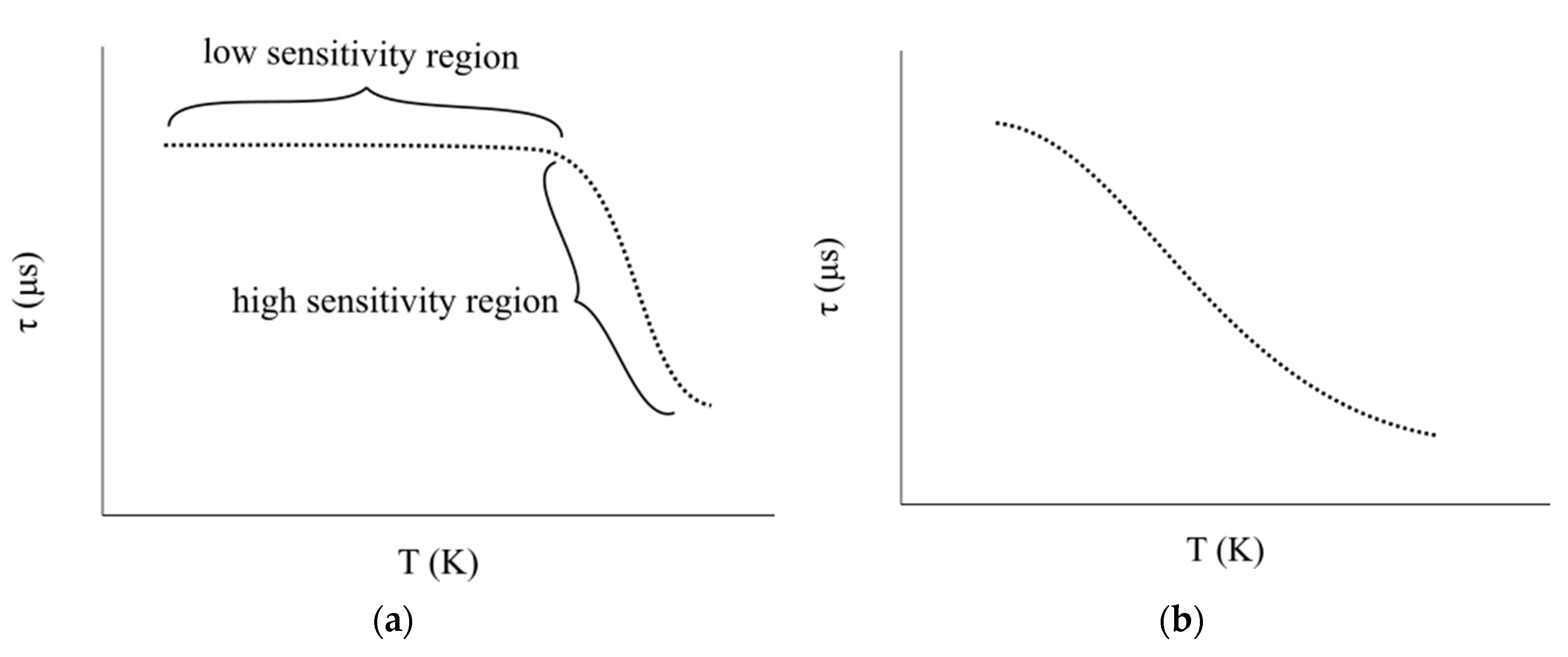
For some systems, the luminescence lifetime τ decreases with increasing temperature. For sensitive higher temperature measurements, it is best to use a chromophore (a) for which is large (e.g., Ln3+ doped materials such as YAG:Dy3+ (see Figure 8 Ref. [19]). For sensitive lower temperature measurements, it is best to use a chromophore (b) for which is large at lower temperatures (e.g., ruby, Al2O3:Cr3+) [34,35,36].
Figure 16.
For some systems, the luminescence lifetime τ decreases with increasing temperature. For sensitive higher temperature measurements, it is best to use a chromophore (a) for which is large (e.g., Ln3+ doped materials such as YAG:Dy3+ (see Figure 8 Ref. [19]). For sensitive lower temperature measurements, it is best to use a chromophore (b) for which is large at lower temperatures (e.g., ruby, Al2O3:Cr3+) [34,35,36].

Figure 17.
Luminescent quantum dots (QDs) showing the correlations between quantum dot size, the band gap between the conduction (CB) and valence bands (VB), and the photon emission energy.
Figure 17.
Luminescent quantum dots (QDs) showing the correlations between quantum dot size, the band gap between the conduction (CB) and valence bands (VB), and the photon emission energy.

Figure 18.
Schematic of near IR luminescence spectra of PbSe QDs showing peak wavelength and intensity trends: peak wavelengths λ1 < λ2 < λ3, peak intensities I1 > I2 > I3.
Figure 18.
Schematic of near IR luminescence spectra of PbSe QDs showing peak wavelength and intensity trends: peak wavelengths λ1 < λ2 < λ3, peak intensities I1 > I2 > I3.

Figure 19.
Diagram of octahedral site of the Cr3+ cation and six O2− nearest neighbor ligating anions in ruby.
Figure 19.
Diagram of octahedral site of the Cr3+ cation and six O2− nearest neighbor ligating anions in ruby.

Figure 20.
Splitting of the 2E excited state of ruby gives rise to two closely spaced luminescence bands designated R1 and R2. These bands shift in wavelengths as a function of temperature and also as a function of pressure. At room temperature and pressure λ(R1) = 694.3 nm and λ(R2) = 692.7 nm. The ruby temperature calibration range extends from 15–600 K. Increasing pressure redshifts both the R1 and R2 luminescence bands. The standard values for the R line shift are +0.0365 nm kbar−1 [54].

Figure 21.
Schematic of two-photon luminescence upconversion spectroscopy. Two low-energy excitation photons penetrate to the desired tissue depth owing to the minimization of Rayleigh scattering and tissue absorption. These photons then combine to yield a single high-energy emission photon that can be used as a laser scalpel to destroy a tumor or an individual cell.

Publisher’s Note: MDPI stays neutral with regard to jurisdictional claims in published maps and institutional affiliations. |
© 2021 by the authors. Licensee MDPI, Basel, Switzerland. This article is an open access article distributed under the terms and conditions of the Creative Commons Attribution (CC BY) license (https://creativecommons.org/licenses/by/4.0/).
Share and Cite
MDPI and ACS Style
Kenney, J.W., III; Lee, J.J. Photoluminescent Metal Complexes and Materials as Temperature Sensors—An Introductory Review. Chemosensors 2021, 9, 109. https://0-doi-org.brum.beds.ac.uk/10.3390/chemosensors9050109
AMA Style
Kenney JW III, Lee JJ. Photoluminescent Metal Complexes and Materials as Temperature Sensors—An Introductory Review. Chemosensors. 2021; 9(5):109. https://0-doi-org.brum.beds.ac.uk/10.3390/chemosensors9050109
Chicago/Turabian StyleKenney, John W., III, and Jae Joon Lee. 2021. "Photoluminescent Metal Complexes and Materials as Temperature Sensors—An Introductory Review" Chemosensors 9, no. 5: 109. https://0-doi-org.brum.beds.ac.uk/10.3390/chemosensors9050109
Note that from the first issue of 2016, this journal uses article numbers instead of page numbers. See further details here.