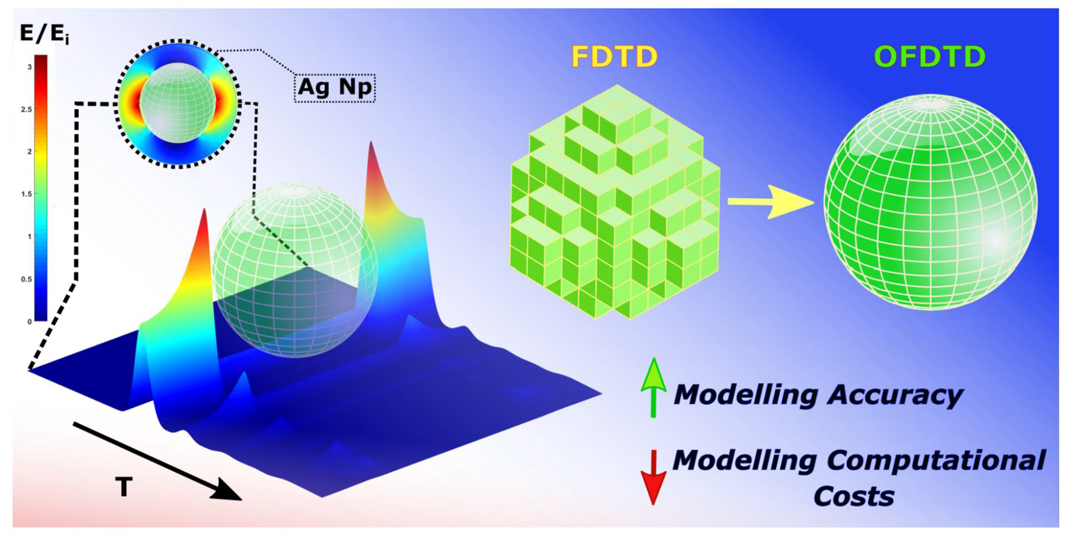
Optimized 3D Finite-Difference-Time-Domain Algorithm to Model the Plasmonic Properties of Metal Nanoparticles with Near-Unity Accuracy

Abstract

The finite difference time domain (FDTD) method is a grid-based, robust, and straightforward method to model the optical properties of metal nanoparticles (MNPs). Modelling accuracy and optical properties can be enhanced by increasing FDTD grid resolution; however, the resolution of the grid size is limited by the memory and computational requirements. In this paper, a 3D optimized FDTD (OFDTD) was designed and developed, which introduced new FDTD approximation terms based on the physical events occurring during the plasmonic oscillations in MNP. The proposed method not only required ~52% less memory than conventional FDTD, but also reduced the calculation requirements by ~9%. The 3D OFDTD method was used to model and obtain the extinction spectrum, localized surface plasmon resonance (LSPR) frequency, and the electric field enhancement factor (EF) for spherical silver nanoparticles (Ag NPs). The model’s predicted results were compared with traditional FDTD as well as experimental results to validate the model. The OFDTD results were found to be in excellent agreement with the experimental results. The EF accuracy was improved by 74% with respect to FDTD simulation, which helped reaching a near-unity OFDTD accuracy of ~99%. The ${\lambda }_{LSPR}$ discrepancy reduced from 20 nm to 3 nm. The EF peak position discrepancy improved from ±5.5 nm to only ±0.5 nm.

1. Introduction

Plasmonic properties of MNPs are due to the collective response of electromagnetic radiation induced oscillations in conduction band electrons [1]. In the absence of an external electric field, the electron cloud is symmetrically distributed around the nuclei. When an external electric field, such as the one associated with the electromagnetic spectrum, is applied, the electrons and positively charged nuclei are polarized. This displaces the electron cloud from positively charged nuclei, and, as a result, forms a dipole, which creates a restoring force and oscillates with a certain frequency known as plasmon frequency. It is known as the electromagnetic excitation and oscillation of the conduction electron, which is characterized by the resonance frequency of the MNP, referred to as surface plasmon resonance (SPR) [2]. The oscillations experience a damping force due to electron collisions (characterized by the collision frequency of MNP). SPR is an evanescently confined electromagnetic excitation, which propagates perpendicularly at the interface between a dielectric and a conductor [2]. In small and sub-wavelength MNPs, plasmonic resonance is confined locally, and known as LSPR. This confines the electromagnetic excitation electric field in the subwavelength range and, consequently, induces a remarkable local amplification in electric field intensity. This enhanced electric field strength decay from MNP surface is broadly divided into near-field and far-field response of MNPs. The latter is responsible for macroscopic properties such as the color resulting from the MNP, while the near-field response is more important in controlling and manipulating the optical properties of the MNP, such as in near-field scattering in plasmonic coupling applications [3,4,5,6,7,8].

The strong LSPR in MNPs makes them a good choice for many applications in optical and photonic fields [1,6,8,9,10,11,12,13,14,15,16,17,18,19,20,21,22,23,24,25,26,27,28]. Among the noble metals, the LSPR of gold and silver were the most studied for the following reasons: Their near-field oscillation energy is high due to the very small imaginary part of their dielectric function, which has a direct correlation with the extinction coefficient and the optical absorption of the MNPs. The LSPR frequency of these MNPs can be tuned by their size, shape, and local environment specifications. Their LSPR frequency is in the visible range of the spectrum; hence, the plasmonic properties can be easily excited by solar radiation, unlike other metals’ plasma frequency (such as Hg, In, Pb, Cd, and Sn). They are chemically inert, allowing them to be chemically stable. They do not oxidize, while the oxidation in other metals changes their LSPR frequency. They can be coupled with fluorescent molecules to improve their optical properties in luminescent solar concentrators and down shifting layers [25,26,27,28]. Similarly, they can be easily attached to bio molecules using chemical linkers.

Theoretically, evaluating the optical properties and the optical response of MNP requires a well-defined computational strategy. Purcell and Pennypacker introduced a discrete dipole approximation (DDA) method [29] to model the optical properties of MNPs. The number of numerical and theoretical methods have been developed, since then, to solve Maxwell’s equations (see Supplementary Materials for more details) in either frequency domain or time domain, such as the boundary element method (BEM), spectral method (SM), finite element method (FEM), methods of moments (MOM), finite volume method (FVM), and the finite difference time domain (FDTD) method, to model the optical properties of MNPs [30,31,32,33].

Among these, the FDTD method is the most used and developed algorithm, and models the optical properties of MNPs in a Yee grid [34]. Researchers have used the FDTD method to estimate and predict the extinction spectra of the MNPs by changing their size, shape, and concentrations [7,16,35,36,37].

Table 1. The advantages and disadvantages of existing FDTD methods.

Existing FDTD Advantages

Existing FDTD Drawbacks

Easy to understand and develop (simple parametrization and implementation) Excellent for large-scale and transient simulations Accurate, robust, and mature method Easy to debug and find the errors in program Capacity to handle non-linear and anisotropic behavior Ability to analyze the optical properties of complex nanoparticles (such as nano stars)

Simulation accuracy is dependent on $N_{\lambda }$, $\mathsf{\Delta }d$ and time step. Computational time (time steps) is dependent on component dimensions, $N_{\lambda }$ and $\mathsf{\Delta }d$ Required memory of the program is dependent on the component dimensions, $N_{\lambda }$ and $\mathsf{\Delta }d$. Therefore, for achieving high accuracy, both the memory size and simulation time must be increased. The algorithm is more complex to simulate the curved surface where a high $N_{\lambda }$ is required

summarizes the advantages and disadvantages of conventional FDTD methods [16,30]. The drawbacks listed in Table 1 can have an impact on the accuracy of FDTD simulation, especially in plasmonically enhanced solar devices [25,26,27,28,38,39,40]. The accuracy of FDTD models can be characterized by the Yee grid resolution ($N_{\lambda }$) determining the Yee grid discretization ($\mathsf{\Delta }d$), which is the size of each grid cell in x, y, and z vectors (see Equation (S6) and Equation (S7) in Supplementary Materials for more details). The grid discretization is also in correlation with the simulation time step (i.e., the time which is required for the electromagnetic wave, with the smallest wavelength, to pass a single grid cell) based on the Courant stability condition [41] (see Equation (S5) in Supplementary Materials for more details). In the absence of these rules in designing the Yee grid, the FDTD algorithm is not able to accurately model the optical properties of MNP. Although $N_{\lambda }$ of ~20 to 30 is enough for low contrast dielectric modelling [42], in plasmonic coupling application, high $N_{\lambda }$ of ~100 to 200 is required to achieve reasonable accuracy due to the high SPR frequency of radiation inside the grid. This creates the spatial $\mathsf{\Delta }d$ range of only a few nanometers for modelling plasmonic devices under solar radiation conditions.

Our developed FDTD model and its predicted results have already been validated for various sizes, shapes, and concentrations of MNP [39,40]. In this paper, a 3D OFDTD model is developed to overcome the disadvantages of traditional FDTD methods. In the OFDTD, a new set of approximation terms is developed considering physical events occurring during the electromagnetic interaction with MNP. Unlike the traditional FDTD, OFDTD requires less calculation and memory to solve Maxwell’s equations. OFDTD considers identical material conductivity in the 3D vectors of the Yee grid. In the traditional method, the FDTD calculations are applied to the whole MNP grid. Whereas the OFDTD algorithm bypasses identical and repetitive calculations; even though all iterations are counted in the final simulation results. This results in reducing the required memory and calculations in the simulation. Using the new approximation terms in OFDTD resulted in saving ~52% memory, allowing the model to increase the resolution of the Yee grid, which enhanced the modelling performance and output accuracy. The developed OFDTD was used to model the plasmonic effect and optical properties of an isotropic device doped with Ag NPs. The results were compared with the existing FDTD as well as experimental results for validation. The OFDTD predicted output was found to be in very close agreement with experimental results and has achieved higher accuracy in comparison with the FDTD method.

2. Materials and Methods

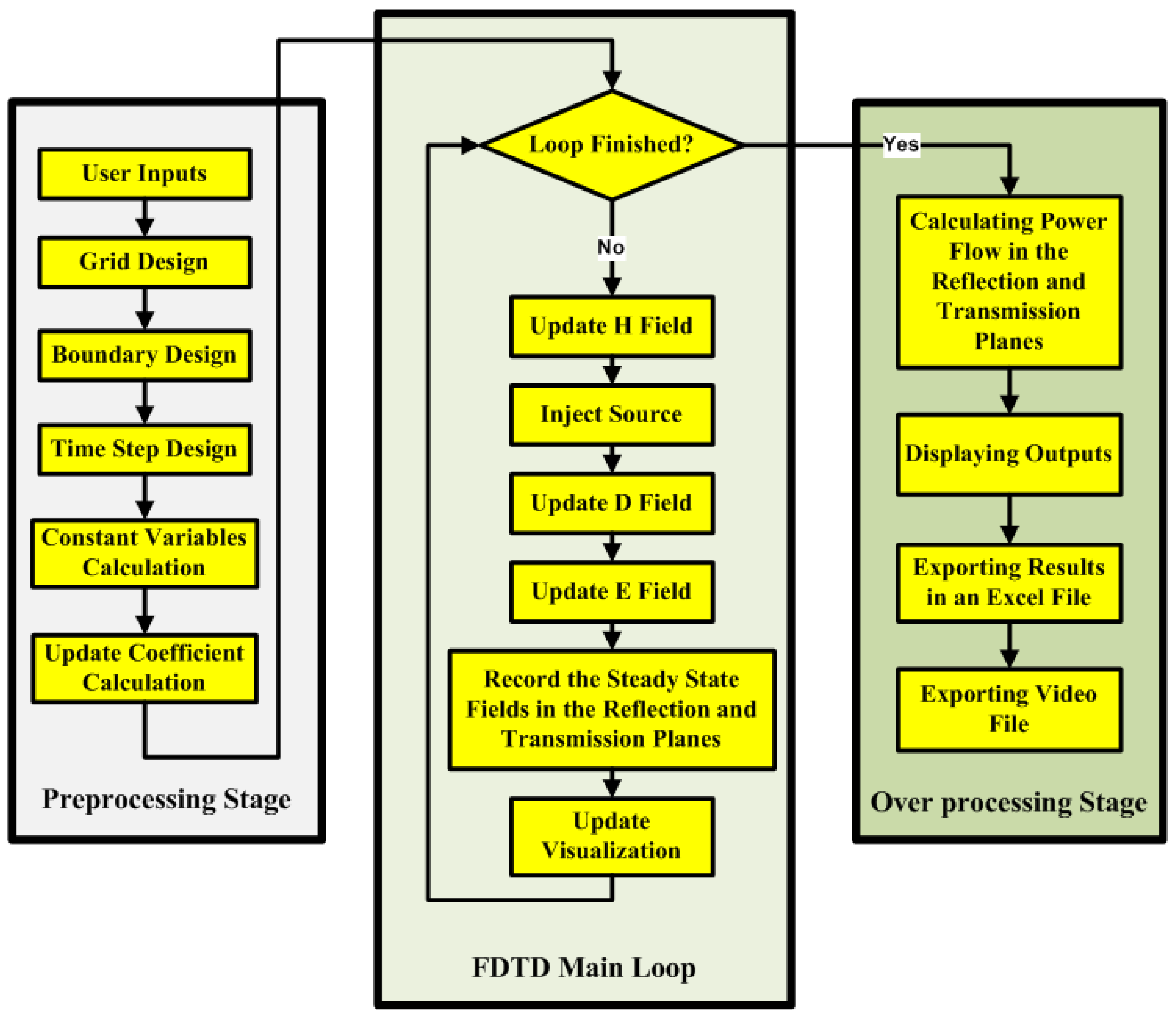
2.1. OFDTD Method Development for Plasmonic Effect Modelling

Figure 1 shows the flowchart developed for applying both FDTD and OFDTD algorithms in this study. As can be seen, it is separated into the three stages of pre-processing, main loop, and over-processing. The pre-processing stage is used in order to apply the user inputs (such as dimensions, type, and shape of MNP, and device configuration) and to design the Yee grid, boundary conditions, simulation time step, the constant values such as $N_{\lambda }$ and $\mathsf{\Delta }d$, the total number of iterations of the main loop, the update coefficients terms, and the constitutive relations (see Supplementary Material for more details).

Thereafter, in each iteration of the main loop, Maxwell’s equations are solved for the Yee grid. Maxwell’s equations are updated based on the leapfrog process, i.e., the magnetic field (H (A/m)) is solved for one time-instant, and the electric field (E (V/m)) is updated at the following time-instant, while the irradiated source field is injected during the updating process. At the end of each iteration, the time domain value of the fields is stored and used in the next time-instant (next iteration).

After implementing the method for the total number of iterations, the algorithm enters the over-processing step, where the power flow and the optical properties of the device (such as reflection, transmission, extinction spectra, and EF) are calculated and exported by transferring the value of fields from time to frequency domain using fast Fourier transform (FFT).

The 3D FDTD terms used in Maxwell’s equations including m, σ, I, C, E, H, D, $\epsilon$, and $\mu$ (see Supplementary Materials for more details about these parameters) are defined as 3D matrices in the model, in which i, j, and k indicate the MNP grid cell location (in the x, y, and z vectors, respectively) in a 3D Yee grid. The size of these 3D matrices is equal to the size of the designed Yee grid, which can be expanded by increasing the resolution and/or the size of the modelled MNP. $\epsilon$ is MNP permittivity in F/m, and $\mu$ is permeability in H/m, while D is electric flux density (also called dielectric displacement) in C/m². m terms are constitutive relations used as update coefficients in the FDTD main loop. I terms are integration terms of the fields, which are the summation of curl (C) terms of the fields.

The electric field inside the MNP is constant during the SPR oscillations. Conductivity ($\sigma$(1/Ω)) is used to apply the amount of electric and magnetic field losses in the MNP and its surrounding area (i.e., in the Yee grid). In physics, by considering an isotropic medium for MNP, magnetic and electric field losses can be considered identical at all x, y, and z vectors. Therefore, in the OFDTD matrix group of $\sigma$, all loss terms for H and D fields in x, y, and z were considered identical and called as ${\sigma }_{xyz}^{HD}{|}^{i,j,k}$, i.e.,:

$${\sigma }_{xyz}^{HD}{|}^{i,j,k}={\sigma }_x^H{|}^{i,j,k}={\sigma }_y^H{|}^{i,j,k}={\sigma }_z^H{|}^{i,j,k}={\sigma }_x^D{|}^{i,j,k}={\sigma }_y^D{|}^{i,j,k}={\sigma }_z^D{|}^{i,j,k}$$

(1)

This resulted in an identical damping rate (${\Gamma }_m$) for the MNP in all vectors. The ${\Gamma }_m$ determined the SPR oscillations and its decay frequency in the polarized direction of MNP. It also characterized MNP permittivity (according to Equation (S10) in Supplementary Materials). Therefore, in OFDTD, the $\epsilon$ terms were also considered to be identical in x, y, and z in the polarized MNP. In addition, the magnetic response of MNP is negligible, i.e., its relative permeability ($\mu$ terms) is almost equal to 1 in all vectors. Under the aforementioned isotropic conditions, new ${\epsilon }_{xyz}{|}^{i,j,k}$ and ${\mu }_{xyz}{|}^{i,j,k}$ matrices can be introduced as:

$$\begin{gathered} {\epsilon }_{xyz}{|}^{i,j,k}={\epsilon }_{xx}{|}^{i,j,k}={\epsilon }_{yy}{|}^{i,j,k}={\epsilon }_{zz}{|}^{i,j,k} \\ {\mu }_{xyz}{|}^{i,j,k}={\mu }_{xx}{|}^{i,j,k}={\mu }_{yy}{|}^{i,j,k}={\mu }_{zz}{|}^{i,j,k} \end{gathered}$$

(2)

Therefore, the 3D ${\tilde{\epsilon }}_r$ and ${\tilde{\mu }}_r$ matrices can be written in isotropic form:

$$\begin{gathered} {\tilde{\epsilon }}_r=\left[\begin{array}{ccc}{\epsilon }_{xx}{|}^{i,j,k}& 0& 0\\ 0& {\epsilon }_{yy}{|}^{i,j,k}& 0\\ 0& 0& {\epsilon }_{zz}{|}^{i,j,k}\end{array}\right]=\left[\begin{array}{ccc}{\epsilon }_{xyz}{|}^{i,j,k}& 0& 0\\ 0& {\epsilon }_{xyz}{|}^{i,j,k}& 0\\ 0& 0& {\epsilon }_{xyz}{|}^{i,j,k}\end{array}\right] \\ {\tilde{\mu }}_r=\left[\begin{array}{ccc}{\mu }_{xx}{|}^{i,j,k}& 0& 0\\ 0& {\mu }_{yy}{|}^{i,j,k}& 0\\ 0& 0& {\mu }_{zz}{|}^{i,j,k}\end{array}\right]=\left[\begin{array}{ccc}{\mu }_{xyz}{|}^{i,j,k}& 0& 0\\ 0& {\mu }_{xyz}{|}^{i,j,k}& 0\\ 0& 0& {\mu }_{xyz}{|}^{i,j,k}\end{array}\right] \end{gathered}$$

(3)

By applying these new isotropic terms (i.e., updated $\sigma$, ${\tilde{\epsilon }}_r$, and ${\tilde{\mu }}_r$), the updated coefficients of the traditional FDTD loop (m terms, which are mentioned in Supplementary Materials) can be optimized and reduced to new isotropic terms for the OFDTD algorithm:

$$\begin{gathered} m_{HDxyz0}{|}^{i,j,k}=m_{Hx0}{|}^{i,j,k}=m_{Hy0}{|}^{i,j,k}=m_{Hy0}{|}^{i,j,k} \\ =m_{Dx0}{|}^{i,j,k}=m_{Dy0}{|}^{i,j,k}=m_{Dz0}{|}^{i,j,k} \\ =\frac{1}{\Delta t}+{\sigma }_{xyz}^{HD}{|}^{i,j,k}\left(\frac{1}{{\epsilon }_0}+\frac{{\sigma }_{xyz}^{HD}{|}^{i,j,k}\Delta t}{4{\epsilon }_0^2}\right) \\ {m}_{HDxyz1}{|}^{i,j,k}=m_{Hx1}{|}^{i,j,k}=m_{Hy1}{|}^{i,j,k}=m_{Hy1}{|}^{i,j,k} \\ =m_{Dx1}{|}^{i,j,k}=m_{Dy1}{|}^{i,j,k}=m_{Dz1}{|}^{i,j,k} \\ =m_{HDxyz1}[\frac{1}{\Delta t}-{\sigma }_{xyz}^{HD}{|}^{i,j,k}\left(\frac{1}{{\epsilon }_0}+\frac{{\sigma }_{xyz}^{HD}{|}^{i,j,k}\Delta t}{4{\epsilon }_0^2}\right)] \\ {m}_{Hxyz2}{|}^{i,j,k}=m_{Hx2}{|}^{i,j,k}=m_{Hy2}{|}^{i,j,k}=m_{Hy2}{|}^{i,j,k}=-\frac{1}{m_{HDxyz0}{|}^{i,j,k}}\frac{c_0}{{\mu }_{xyz}{|}^{i,j,k}} \\ {m}_{Hxyz3}{|}^{i,j,k}=m_{Hx3}{|}^{i,j,k}=m_{Hy3}{|}^{i,j,k}=m_{Hy3}{|}^{i,j,k} \\ =-\frac{1}{m_{HDxyz0}{|}^{i,j,k}}\frac{c_0\Delta t}{{\epsilon }_0}\frac{{\sigma }_{xyz}^{HD}{|}^{i,j,k}}{{\mu }_{xyz}{|}^{i,j,k}} \\ {m}_{HDxyz4}{|}^{i,j,k}=m_{Hx4}{|}^{i,j,k}=m_{Hy4}{|}^{i,j,k}=m_{Hy4}{|}^{i,j,k} \\ =m_{Dx4}{|}^{i,j,k}=m_{Dy4}{|}^{i,j,k}=m_{Dz4}{|}^{i,j,k} \\ =-\frac{1}{m_{HDxyz0}{|}^{i,j,k}}\frac{\Delta t}{{\epsilon }_0^2}{\left({\sigma }_{xyz}^{HD}{|}^{i,j,k}\right)}^2 \\ {m}_{Dxyz2}{|}^{i,j,k}=m_{Dx2}{|}^{i,j,k}=m_{Dy2}{|}^{i,j,k}=m_{Dz2}{|}^{i,j,k}=\frac{c_0}{m_{HDxyz0}{|}^{i,j,k}} \\ {m}_{Dxyz2}{|}^{i,j,k}=m_{Dx2}{|}^{i,j,k}=m_{Dy2}{|}^{i,j,k}=m_{Dz2}{|}^{i,j,k}=\frac{c_0}{m_{HDxyz0}{|}^{i,j,k}} \\ {m}_{Dxyz3}{|}^{i,j,k}=m_{Dx3}{|}^{i,j,k}=m_{Dy3}{|}^{i,j,k}=m_{Dz3}{|}^{i,j,k}=\frac{1}{m_{HDxyz0}{|}^{i,j,k}}\frac{c_0\Delta t}{{\epsilon }_0}{\sigma }_{xyz}^{HD}{|}^{i,j,k} \\ {m}_{Exyz1}{|}^{i,j,k}=m_{Ex1}{|}^{i,j,k}=m_{Ey1}{|}^{i,j,k}=m_{Ez1}{|}^{i,j,k}=\frac{1}{{\epsilon }_{xyz}{|}^{i,j,k}} \end{gathered}$$

(4)

The reduction in size of the OFDTD terms reduced the memory requirements.

Table 2. Equal 3D matrix groups in the FDTD modelling can be replaced by only a single alternative 3D matrix in OFDTD, which reduces the required memory for the group.

	Type of the Matrix Group	Equal Matrix Group	Alternative Matrix	Required Memory Deduction of Matrix Group (%)	$\mathbf{Optimization}\mathbf{Factor}\mathbf{of}\mathbf{Matrix}\mathbf{Group}\left({\mathit{f}}_{\mathit{i}}^{\mathit{O}\mathit{P}\mathit{T}}\right)$
1	$\sigma$ terms	${\sigma }_x^H{|}^{i,j,k}$, ${\sigma }_y^H{|}^{i,j,k}$, ${\sigma }_z^H{|}^{i,j,k}$ ${\sigma }_x^D{|}^{i,j,k}$, ${\sigma }_y^D{|}^{i,j,k}$, ${\sigma }_z^D{|}^{i,j,k}$	${\sigma }_{xyz}^{HD}{|}^{i,j,k}$	84%	$\frac{1}{6}$
2	H and D update coefficient m0 terms	$m_{Hx0}{|}^{i,j,k}$, $m_{Hy0}{|}^{i,j,k}$, $m_{Hz0}{|}^{i,j,k}$, $m_{Dx0}{|}^{i,j,k}$, $m_{Dy0}{|}^{i,j,k}$, $m_{Dz0}{|}^{i,j,k}$	$m_{HDxyz0}{|}^{i,j,k}$	84%	$\frac{1}{6}$
3	H and D update coefficient m1 terms	$m_{Hx1}{|}^{i,j,k}$, $m_{Hy1}{|}^{i,j,k}$, $m_{Hz1}{|}^{i,j,k}$, $m_{Dx1}{|}^{i,j,k}$, $m_{Dy1}{|}^{i,j,k}$, $m_{Dz1}{|}^{i,j,k}$	$m_{HDxyz1}{|}^{i,j,k}$	84%	$\frac{1}{6}$
4	H update coefficient m2 terms	$m_{Hx2}{|}^{i,j,k}$, $m_{Hy2}{|}^{i,j,k}$, $m_{Hz2}{|}^{i,j,k}$	$m_{Hxyz2}{|}^{i,j,k}$	67%	$\frac{1}{3}$
5	H update coefficient m3 terms	$m_{Hx3}{|}^{i,j,k}$, $m_{Hy3}{|}^{i,j,k}$, $m_{Hz3}{|}^{i,j,k}$	$m_{Hxyz3}{|}^{i,j,k}$	67%	$\frac{1}{3}$
6	H and D update coefficient m4 terms	$m_{Hx4}{|}^{i,j,k}$, $m_{Hy4}{|}^{i,j,k}$, $m_{Hz4}{|}^{i,j,k}$, $m_{Dx4}{|}^{i,j,k}$, $m_{Dy4}{|}^{i,j,k}$, $m_{Dz4}{|}^{i,j,k}$	$m_{HDxyz4}{|}^{i,j,k}$	84%	$\frac{1}{6}$
7	D update coefficient m2 terms	$m_{Dx2}{|}^{i,j,k}$, $m_{Dy2}{|}^{i,j,k}$, $m_{Dz2}{|}^{i,j,k}$	$m_{Dxyz2}{|}^{i,j,k}$	67%	$\frac{1}{3}$
8	D update coefficient m3 terms	$m_{Dx3}{|}^{i,j,k}$, $m_{Dy3}{|}^{i,j,k}$, $m_{Dz3}{|}^{i,j,k}$	$m_{Dxyz3}{|}^{i,j,k}$	67%	$\frac{1}{3}$
9	E update coefficient m terms	$m_{Ex1}{|}^{i,j,k}$, $m_{Ey1}{|}^{i,j,k}$, $m_{Ez1}{|}^{i,j,k}$	$m_{Exyz1}{|}^{i,j,k}$	67%	$\frac{1}{3}$
10	${\tilde{\epsilon }}_r$ terms	${\epsilon }_{xx}{|}^{i,j,k}$, ${\epsilon }_{yy}{|}^{i,j,k}$, ${\epsilon }_{zz}{|}^{i,j,k}$	${\epsilon }_{xyz}{|}^{i,j,k}$	67%	$\frac{1}{3}$

classifies the achieved OFDTD terms and the matrix groups. As is seen in Equation (4) and Table 2, in the matrix group of $\sigma$, FDTD terms for H and D fields in x, y, and z were replaced with one single alternative 3D matrix (${\sigma }_{xyz}^{HD}{|}^{i,j,k}$) in the OFDTD algorithm. This resulted in a reduction of 84% of the required memory for $\sigma$ matrix group. For ${\tilde{\epsilon }}_r$ matrix group, the three permittivity terms were replaced with a single 3D matrix (${\epsilon }_{xyz}{|}^{i,j,k}$) in OFDTD, which led to a ~67% deduction in the required memory for the relative permittivity group. The same optimization process was applied for the update coefficient matrix groups (m terms). For example, m0 update coefficients for D and H fields could be replaced with an alternative matrix,$m_{HDxyz0}{|}^{i,j,k}$, in OFDTD. This has resulted in an 84% deduction in the memory required for these matrix groups. Moreover, during the simulation process, the m0 terms in Equation (4) were calculated only once instead of the six times in Equation (S2) and Equation (S3) (in Supplementary Materials), which could significantly reduce the computational requirements.

The estimated rate of the total required memory, which was deducted using the OFDTD algorithm, was calculated by:

$$\Delta ME{M}_{Total}=\frac{ME{M}_{Total}-[{{\displaystyle \sum }}_{i=1}^M{f}_i^{OPT}\times ME{M}_i]}{ME{M}_{Total}}\times 100$$

(5)

where $ME{M}_{Total}$ is the total memory size that is used in the 3D FDTD algorithm, M is the total number of equal matrix groups (which is 10 here), and i is the index of each matrix groups. $ME{M}_i$ is the total memory size required for each matrix group. $f_i^{OPT}$ is the optimization factor for the matrix group i, which can be calculated by using the total number of matrices in each matrix group ($N_i^G$):

$$f_i^{OPT}=\frac{1}{N_i^G}$$

(6)

By using the OFDTD, the saving in calculation and memory ($\Delta ME{M}_{Total}$) can allow the MNP to be modelled with a higher resolution of the Yee grid, resulting in a higher accuracy in the modelling outputs.

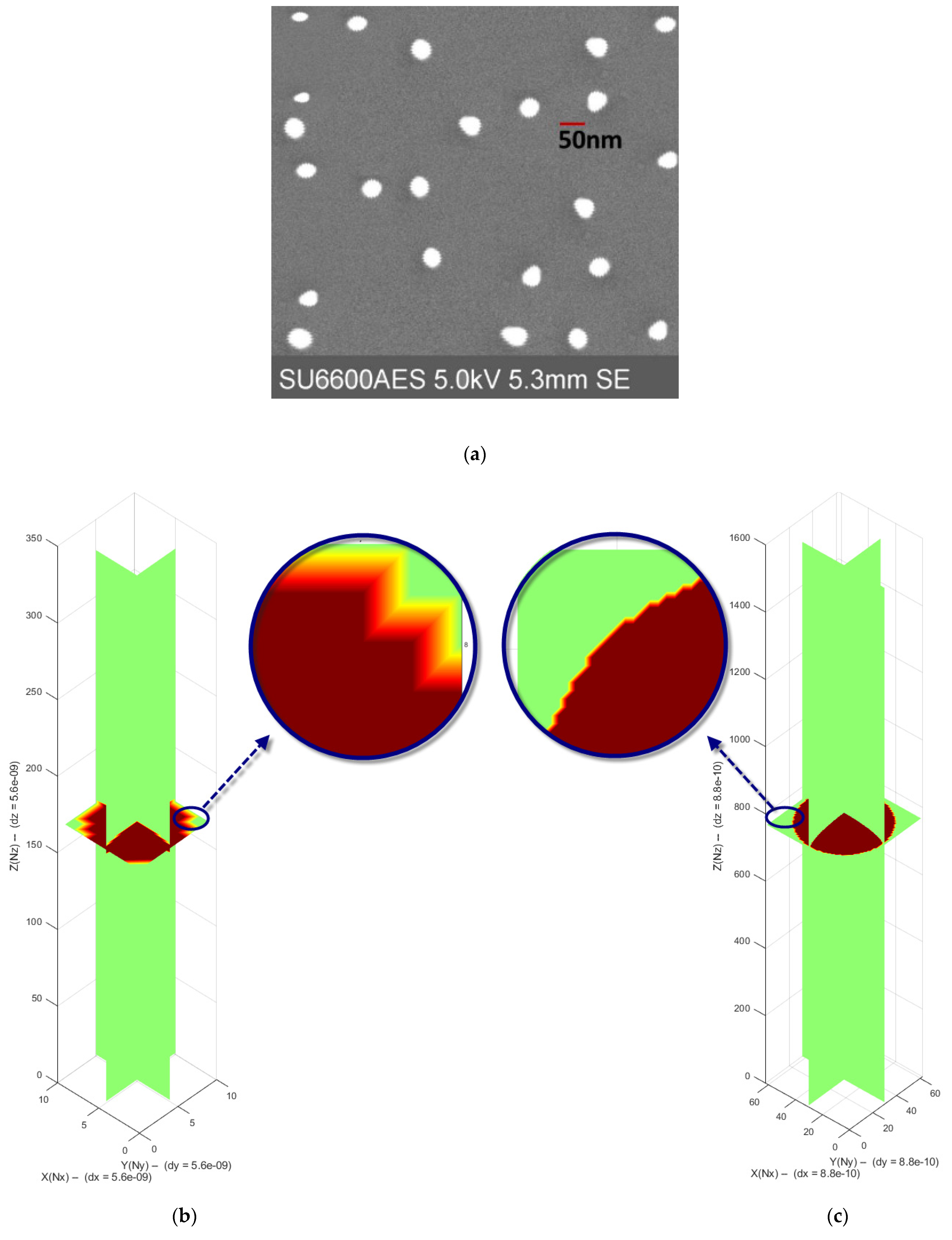
2.2. Description of Samples and Experimental Measurements

Experimental results [43] were used to validate and compare the performance of the FDTD and OFDTD methods. The preparation of a silver colloidal solution was based on the reduction of silver ions by ascorbic acid in the presence of citrate-stabilized silver seed, additional trisodium citrate, and the capping agent polyvinylpyrrolidone. The color of the Ag NPs was controlled by varying the concentration of the trisodium citrate [44]. Scanning electron microscopy (SEM) image of the sample using spherical Ag NPs (with the diameter of ~50 nm) can be seen in Figure 2a, which was obtained using the Hitachi SU6600 FESEM (Trinity College Dublin, Ireland) at an accelerating voltage of 5 kV. UV/Vis extinction spectra of Ag NP particles extracted from water can be seen in Figure 3 (labeled as Reference), which was used as the experimental reference extinction spectrum in this study.

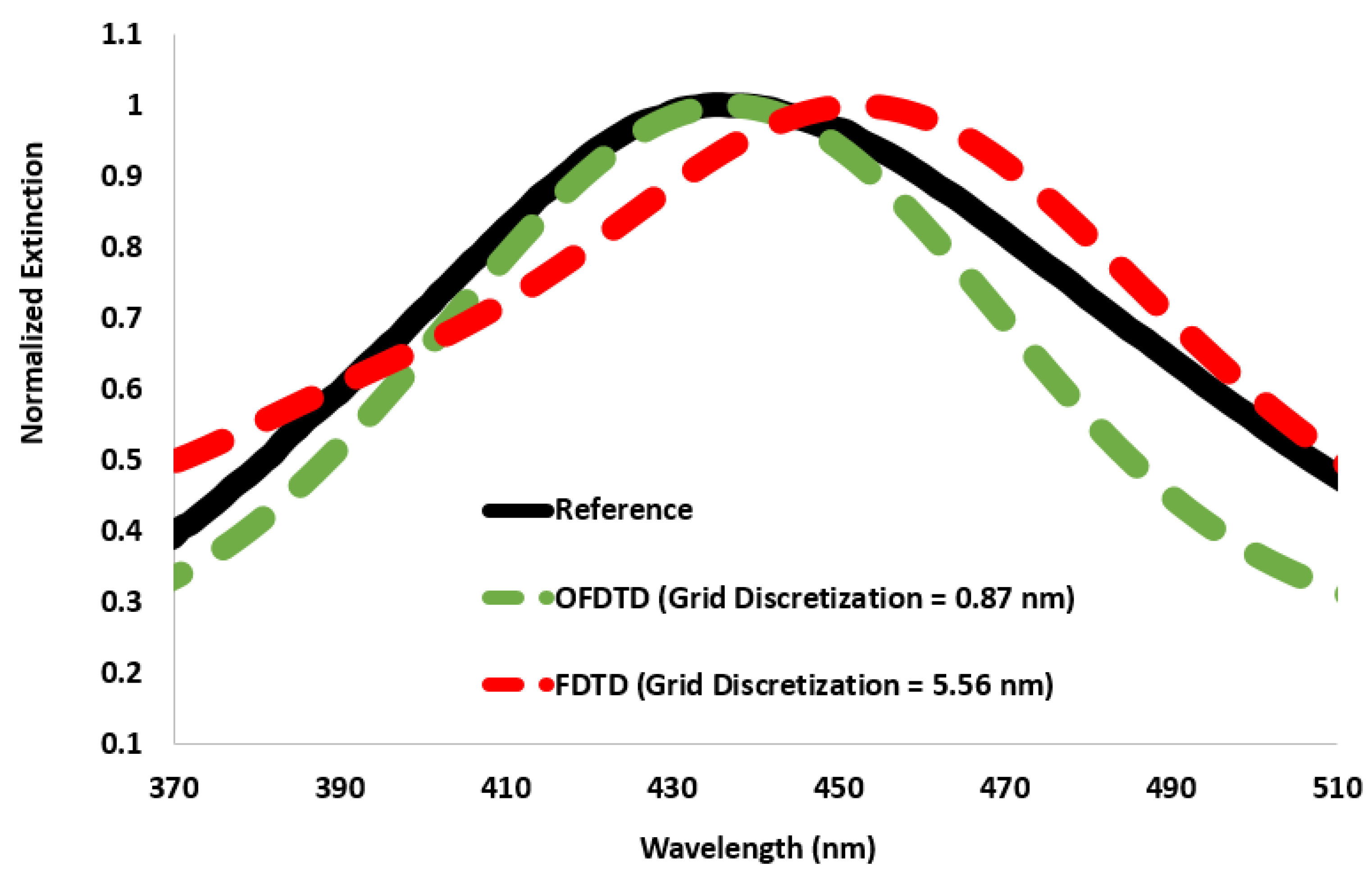
3. Results and Discussion

Figure 2b shows the modelled Ag NP in a 3D FDTD Yee grid, where $\Delta d=5.56$ nm and the total grid size was 10 × 10 × 330. The time step was $\Delta t=1.070\times {10}^{-17}\mathrm{s}$. Periodic boundary conditions were defined at the x and y axes, while scattering boundary conditions were defined at the z axis by placing perfectly matched layers (PML) at both ends of the grid in the z axis. PML was designed by using the field termination function of:

$$F_T\left(z\right)=\frac{{\epsilon }_0}{2\Delta t}{\left(\frac{z}{L}\right)}^3$$

(7)

where ∆t is the time step in second, L is the length of the PML in m, and ${\epsilon }_0\approx 8.86\times {10}^{-12}$ F/m is free-space permittivity. The length of the PML (280 nm) should be designed so that it is able to absorb and terminate the total electrical field striking the absorbing boundary.

For achieving a higher accuracy, the resolution of the Yee grid had to be increased, which meant that $\Delta d$ had to be reduced. The primary FDTD method was unable to run the simulation for higher resolutions (i.e., grid resolution with $\Delta d<5\mathrm{nm}$); however, the OFDTD was able to model the MNP in a high resolution ($\Delta d=0.877\mathrm{nm}$), which was ~7 times higher than FDTD, as can be seen in Figure 2c. Under this circumstance, the total grid size was 62 × 62 × 1530, and the time step was $\Delta t=1.68\times {10}^{-18}\mathrm{s}$.

Both FDTD and OFDTD models were implemented in a machine with Core [email protected] CPU and 16GB RAM (Trinity College Dublin, Ireland). The modelled samples were illuminated by a Gaussian electric field, which was injected as a plane wave propagated in the z-direction and polarized along the x-y plane. In each time step, the electric field was recorded at the top of the particle where the record plane was placed in the boundary of the study-space and the PML layer. After terminating the irradiation and ending the FDTD main loop, extinction spectra and EF of the Ag NP device were achieved by using FFT and the recorded time-domain electric fields.

Figure 3 shows the normalized extinction spectra obtained by the FDTD and OFDTD methods. They were also compared with the experimental extinction spectra for validation purposes. As can be seen, the FDTD model results did not match with the reference data due to low resolution (large $\Delta d$) of the Yee grid. The LSPR peak wavelengths (${\lambda }_{LSPR}$) obtained by the FDTD model was at $455\mathrm{nm}$ while it was reported at $435\mathrm{nm}$ experimentally. To increase the accuracy, the grid resolution was increased ($\Delta d=0.877\mathrm{nm}$); however, the FDTD method crashed due to high calculations and memory requirements. On the other hand, the OFDTD model could successfully run the simulation with high resolution, where the modeling result (${\lambda }_{LSPR}$ = ~438 nm) were found to be in close agreement with the experimental output (${\lambda }_{LSPR}$ = ~435 nm), with a ~99% accuracy.

The intensity of the incident electric field was significantly enhanced by EF at the surface boundary of the Ag NP due to the excitation of LSPR. EF is calculated by [45,46,47]:

$$EF=\frac{{\left|E\left(x_d,{\lambda }_{ex}\right).e_p\right|}^2}{|E_i{|}^2}$$

(8)

where $E_i$ is the intensity of the incident radiation, ${\lambda }_{ex}$ is the MNP excitation wavelength, and $x_d$ is the place of the particle with a unit dipole moment of $e_p$. Figure 4 compares the achieved EF with the theoretical reference data. As can be seen, FDTD and reference results were not matched; however, by using the OFDTD model, EF reached the peak of ≈10.5 at the surface boundary of MNP, which was in very close agreement with the sharp reference EF. The reference graph in Figure 4 was obtained theoretically by using Equation (8), the intensity of incident radiation and electric field distributed in the grid with $\Delta d=0.812\mathrm{nm}$ where maximum modeling accuracy was achieved. In this case, modeling ${\lambda }_{LSPR}$= ~437 nm (comparing with experimental ${\lambda }_{LSPR}$= ~435 nm), which resulted in a near-unity OFDTD accuracy of ~99%. This was the highest OFDTD accuracy, and applying any $\Delta d$ below $0.812\mathrm{nm}$ (applying higher resolution) could not have any further impact on improving the accuracy.

Detailed and statistical modelling results are presented in

Table 3. Comparison of statistical results obtained by FDTD and OFDTD.

	Low Resolution Condition		High Resolution Condition
$\Delta d$(nm)	5.56		0.877
Method	FDTD	OFDTD	FDTD	OFDTD
Total Yee Grid size (x × y × z)	10 × 10 × 330	10 × 10 × 330	Simulation Crashed Due to High Calculations and Memory Requirements	62 × 62 × 1530
Total Iterations of Main Loop	1505	1505		2743
${\lambda }_{LSPR}$(nm) (Exp. Reference = 435)	455	455		438 (~99% Accuracy)
${\lambda }_{LSPR}$ Discrepancy (nm)	−20	−20		+3
EF Peak (Reference = 10.57)	2.73	2.73		10.52
EF Accuracy (%)	25.8	25.8		99.5
EF Peak Position (nm)(Reference: ±25)	±30.5	±30.5		±24.5
EF Peak Position Discrepancy (nm)	±5.5	±5.5		±0.5
Simulation Time (Hour)	0.74	0.67		121.85
Required Memory (%)	89	42		93
Deduction in Simulation Time in OFDTD (%)	~ 9.4
Deduction in Required Memory in OFDTD (%)	~ 52.8

. It can be seen that by reducing $\Delta d$ from 5.56 nm to 0.877 nm, the number of iterations inside the main loop increased from 1505 to 2743, increasing the simulation time. The results of the FDTD and OFDTD models were similar for low resolution ($\Delta d=$5.56 nm). When high resolution ($\Delta d=$0.877 nm) was used in order to improve the accuracy, the OFDTD model could successfully run the simulation in around 122 h. While this was relatively a long simulation time, it was acceptable considering OFDTD increased accuracy while the FDTD method crashed and was unable to run the simulation. The experimental results were closely matched with the OFDTD high-resolution results. By using OFDTD, the ${\lambda }_{LSPR}$ discrepancy was minimized by 17 nm. The EF peak was 2.73 for the FDTD model and 10.52 (sharp peak) for the OFDTD model. The EF accuracy was improved by 74% with respect to FDTD simulation, which led to a near-unity OFDTD accuracy of ~99%. The EF peak position discrepancy was ±0.5 nm for the OFDTD model while it was ±5.5 nm for FDTD. It was observed that the total amount of memory consumed by OFDTD was ~52% less than the FDTD model. In addition, the optimization steps used in OFDTD offered a ~9% reduction in the simulation time, in comparison with FDTD.

It can be observed that there was a small deviation between the OFDTD and experimental results. The reason for this discrepancy is due to the fact that the Lorentz–Drude relative permittivity spectrum (Equation (S10) in Supplementary Materials) was not perfectly matched with the experimental data achieved by Johnson and Christy [48,49] for Ag NPs. Moreover, the MNPs were considered to be monodisperse (with the same shape) in the model, which were periodically distributed; however, in the experiment, there are some limitations to achieve monodispersity in MNP. In addition, they are also randomly distributed inside the device.

4. Conclusions

Although the FDTD method is an excellent numerical algorithm to solve Maxwell’s equations, its required memory, calculation, and accuracy are dependent on the Yee grid properties of the modelled device. Implementation requirements for MNP modelling are high grid resolution and accuracy. By using the developed 3D OFDTD method, new 3D parameters of the model were developed based on the physical events occurring during the plasmonic excitation in MNPs. The identical calculations were bypassed during the simulation and were replaced with a single alternative parameter. Thus, the OFDTD model not only decreased the total required memory by ~52%, but it also decreased the simulation time by ~9%. This allowed an increase in Yee grid resolution which leads to enhancing the accuracy of the modeling results. The performance of the developed OFDTD method was validated by comparing the simulation and experimental results of a spherical Ag NPs. The traditional FDTD modeling results did not match with the experimental results due to having a low grid resolution. However, for the high-resolution OFDTD model, the extinction spectra and the position of the LSPR wavelength were in very close agreement with the experiment results (~435 nm), which led to the near-unity OFDTD accuracy of ~99%.

References

1. Ritchie, R. Plasma losses by fast electrons in thin films. Phys. Rev. 1957, 106, 874. [Google Scholar] [CrossRef]
2. Maier, S.A. Plasmonics: Fundamentals and Applications; Springer Science & Business Media: Cham, Switzerland, 2007. [Google Scholar]
3. Chicanne, C.; David, T.; Quidant, R.; Weeber, J.-C.; Lacroute, Y.; Bourillot, E.; Dereux, A.; Des Francs, G.C.; Girard, C. Imaging the local density of states of optical corrals. Phys. Rev. Lett. 2002, 88, 097402. [Google Scholar] [CrossRef] [Green Version]
4. Rechberger, W.; Hohenau, A.; Leitner, A.; Krenn, J.; Lamprecht, B.; Aussenegg, F. Optical properties of two interacting gold nanoparticles. Opt. Commun. 2003, 220, 137–141. [Google Scholar] [CrossRef]
5. Grand, J.; Kostcheev, S.; Bijeon, J.-L.; De La Chapelle, M.L.; Adam, P.-M.; Rumyantseva, A.; Lérondel, G.; Royer, P. Optimization of SERS-active substrates for near-field Raman spectroscopy. Synth. Met. 2003, 139, 621–624. [Google Scholar] [CrossRef]
6. Orendorff, C.J.; Sau, T.K.; Murphy, C.J. Shape-Dependent Plasmon-Resonant Gold Nanoparticles. Small 2006, 2, 636–639. [Google Scholar] [CrossRef]
7. Ghosh, S.K.; Pal, T. Interparticle coupling effect on the surface plasmon resonance of gold nanoparticles: From theory to applications. Chem. Rev. 2007, 107, 4797–4862. [Google Scholar] [CrossRef]
8. Haiss, W.; Thanh, N.T.; Aveyard, J.; Fernig, D.G. Determination of size and concentration of gold nanoparticles from UV− Vis spectra. Anal. Chem. 2007, 79, 4215–4221. [Google Scholar] [CrossRef] [PubMed]
9. Efrima, S.; Metiu, H. Classical theory of light scattering by an adsorbed molecule. I. Theory. J. Chem. Phys. 1979, 70, 1602–1613. [Google Scholar] [CrossRef]
10. Aravind, P.; Metiu, H. The enhancement of Raman and fluorescent intensity by small surface roughness. Changes in dipole emission. Chem. Phys. Lett. 1980, 74, 301–305. [Google Scholar] [CrossRef]
11. Gersten, J.; Nitzan, A. Electromagnetic theory of enhanced Raman scattering by molecules adsorbed on rough surfaces. J. Chem. Phys. 1980, 73, 3023–3037. [Google Scholar] [CrossRef]
12. Wang, D.-S.; Chew, H.; Kerker, M. Enhanced Raman scattering at the surface (SERS) of a spherical particle. Appl. Opt. 1980, 19, 2256–2257. [Google Scholar] [CrossRef]
13. Mirkin, C.; Ratner, M. Controlled synthesis and quantum-size effect in gold-coated nanoparticles. Annu. Rev. Phys. Chem. 1997, 101, 1593. [Google Scholar]
14. Rampi, M.A.; Schueller, O.J.; Whitesides, G.M. Alkanethiol self-assembled monolayers as the dielectric of capacitors with nanoscale thickness. Appl. Phys. Lett. 1998, 72, 1781–1783. [Google Scholar] [CrossRef]
15. Scaffardi, L.; Pellegri, N.; De Sanctis, O.; Tocho, J. Sizing gold nanoparticles by optical extinction spectroscopy. Nanotechnology 2004, 16, 158. [Google Scholar] [CrossRef]
16. Myroshnychenko, V.; Rodríguez-Fernández, J.; Pastoriza-Santos, I.; Funston, A.M.; Novo, C.; Mulvaney, P.; Liz-Marzán, L.M.; de Abajo, F.J.G. Modelling the optical response of gold nanoparticles. Chem. Soc. Rev. 2008, 37, 1792–1805. [Google Scholar] [CrossRef] [Green Version]
17. Alvarez, M.M.; Khoury, J.T.; Schaaff, T.G.; Shafigullin, M.N.; Vezmar, I.; Whetten, R.L. Optical absorption spectra of nanocrystal gold molecules. J. Phys. Chem. B 1997, 101, 3706–3712. [Google Scholar] [CrossRef] [Green Version]
18. Lyon, L.A.; Pena, D.J.; Natan, M.J. Surface plasmon resonance of Au colloid-modified Au films: Particle size dependence. J. Phys. Chem. B 1999, 103, 5826–5831. [Google Scholar] [CrossRef]
19. Link, S.; El-Sayed, M.A. Spectral Properties and Relaxation Dynamics of Surface Plasmon Electronic Oscillations in Gold and Silver Nanodots and Nanorods; ACS Publications: Washington, DC, USA, 1999. [Google Scholar]
20. Collin, R. Field Theory of Guided Waves, 2nd ed.; IEEE: Piscataway, NJ, USA, 1990. [Google Scholar]
21. Raether, H. Springer Tracts in Modern Physics; Springer: Berlin/Heidelberg, Germany, 1988; Volume 111. [Google Scholar]
22. Barnes, W.L.; Dereux, A.; Ebbesen, T.W. Surface plasmon subwavelength optics. Nature 2003, 424, 824–830. [Google Scholar] [CrossRef]
23. Moskovits, M. Surface-enhanced spectroscopy. Rev. Mod. Phys. 1985, 57, 783. [Google Scholar] [CrossRef]
24. Metiu, H.; Das, P. The electromagnetic theory of surface enhanced spectroscopy. Annu. Rev. Phys. Chem. 1984, 35, 507–536. [Google Scholar] [CrossRef]
25. Ahmed, H.; Doran, J.; McCormack, S. Increased short-circuit current density and external quantum efficiency of silicon and dye sensitised solar cells through plasmonic luminescent down-shifting layers. Sol. Energy 2016, 126, 146–155. [Google Scholar] [CrossRef]
26. Ahmed, H.; McCormack, S.; Doran, J. External Quantum Efficiency Improvement with Luminescent Downshifting Layers: Experimental and Modelling. Int. J. Spectrosc. 2016, 2016. [Google Scholar] [CrossRef] [Green Version]
27. Ahmed, H.; McCormack, S.; Doran, J. Plasmonic luminescent down shifting layers for the enhancement of CdTe mini-modules performance. Sol. Energy 2017, 141, 242–248. [Google Scholar] [CrossRef]
28. Chandra, S.; Doran, J.; McCormack, S.; Kennedy, M.; Chatten, A. Enhanced quantum dot emission for luminescent solar concentrators using plasmonic interaction. Sol. Energy Mater. Sol. Cells 2012, 98, 385–390. [Google Scholar] [CrossRef] [Green Version]
29. Purcell, E.M.; Pennypacker, C.R. Scattering and absorption of light by nonspherical dielectric grains. Astrophys. J. 1973, 186, 705–714. [Google Scholar] [CrossRef]
30. Inan, U.S.; Marshall, R.A. Numerical Electromagnetics: The FDTD Method; Cambridge University: Cambridge, UK, 2011. [Google Scholar]
31. Taflove, A. Computational Electrodynamics: The Finite-Difference Time-Domain Method; Artech House: Boston, MA, USA, 1995. [Google Scholar]
32. Hao, F.; Nehl, C.L.; Hafner, J.H.; Nordlander, P. Plasmon resonances of a gold nanostar. Nano Lett. 2007, 7, 729–732. [Google Scholar] [CrossRef]
33. Jain, P.K.; Lee, K.S.; El-Sayed, I.H.; El-Sayed, M.A. Calculated absorption and scattering properties of gold nanoparticles of different size, shape, and composition: Applications in biological imaging and biomedicine. J. Phys. Chem. B 2006, 110, 7238. [Google Scholar] [CrossRef] [Green Version]
34. Yee, K. Numerical solution of initial boundary value problems involving Maxwell’s equations in isotropic media. IEEE Trans. Antennas Propag. 1966, 14, 302–307. [Google Scholar]
35. Vial, A.; Grimault, A.-S.; Macías, D.; Barchiesi, D.; de La Chapelle, M.L. Improved analytical fit of gold dispersion: Application to the modeling of extinction spectra with a finite-difference time-domain method. Phys. Rev. B 2005, 71, 085416. [Google Scholar] [CrossRef]
36. Grand, J.; Adam, P.-M.; Grimault, A.-S.; Vial, A.; De La Chapelle, M.L.; Bijeon, J.-L.; Kostcheev, S.; Royer, P. Optical extinction spectroscopy of oblate, prolate and ellipsoid shaped gold nanoparticles: Experiments and theory. Plasmonics 2006, 1, 135–140. [Google Scholar] [CrossRef]
37. Linden, S.; Kuhl, J.; Giessen, H. Controlling the interaction between light and gold nanoparticles: Selective suppression of extinction. Phys. Rev. Lett. 2001, 86, 4688. [Google Scholar] [CrossRef] [PubMed]
38. Chandra, S. Approach to Plasmonic Luminescent Solar Concentration; Dublin Institute of Technology: Dublin, Ireland, 2013. [Google Scholar]
39. Rafiee, M.; Chandra, S.; Ahmed, H.; Barnham, K.; McCormack, S.J. Small and large scale plasmonically enhanced luminescent solar concentrator for photovoltaic applications: Modelling, optimisation and sensitivity analysis. Opt. Express 2021, 29, 15031–15052. [Google Scholar] [CrossRef] [PubMed]
40. Sethi, A.; Rafiee, M.; Chandra, S.; Ahmed, H.; McCormack, S. Unified Methodology for Fabrication and Quantification of Gold Nanorods, Gold Core Silver Shell Nanocuboids, and Their Polymer Nanocomposites. Langmuir 2019, 35, 13011–13019. [Google Scholar] [CrossRef]
41. Courant, R.; Friedrichs, K.; Lewy, H. On the partial difference equations of mathematical physics. IBM J. 1967, 11, 215–234. [Google Scholar] [CrossRef]
42. Atef, E.; Demir, V. The Finite-Difference Time-Domain Method for Electromagnetics with MATLAB Simulations; The Institution of Engineering and Technology: Raleigh, NC, USA, 2016. [Google Scholar]
43. Ahmed, H.; Sc, B.; Sc, M. Materials Characterization and Plasmonic Interaction in Enhanced Luminescent Down-Shifting Layers for Photovoltaic Devices; Dublin Institute of Technology: Dublin, Ireland, 2014. [Google Scholar]
44. Ledwith, D.M.; Whelan, A.M.; Kelly, J.M. A rapid, straight-forward method for controlling the morphology of stable silver nanoparticles. J. Mater. Chem. 2007, 17, 2459–2464. [Google Scholar] [CrossRef]
45. Osinkina, L. Interactions of Molecules in the Vicinity of Gold Nanoparticles; LMU: Munich, Germany, 2014. [Google Scholar]
46. Darvill, D.; Centeno, A.; Xie, F. Plasmonic fluorescence enhancement by metal nanostructures: Shaping the future of bionanotechnology. Phys. Chem. Chem. Phys. 2013, 15, 15709–15726. [Google Scholar] [CrossRef]
47. Soller, T.; Ringler, M.; Wunderlich, M.; Klar, T.; Feldmann, J.; Josel, H.-P.; Markert, Y.; Nichtl, A.; Kürzinger, K. Radiative and nonradiative rates of phosphors attached to gold nanoparticles. Nano Lett. 2007, 7, 1941–1946. [Google Scholar] [CrossRef]
48. Johnson, P.B.; Christy, R.-W. Optical constants of the noble metals. Phys. Rev. B 1972, 6, 4370. [Google Scholar] [CrossRef]
49. Rakić, A.D.; Djurišić, A.B.; Elazar, J.M.; Majewski, M.L. Optical properties of metallic films for vertical-cavity optoelectronic devices. Appl. Opt. 1998, 37, 5271–5283. [Google Scholar] [CrossRef]
Figure 1. Practical block diagram used for implementing both FDTD and OFDTD algorithm.
Chemosensors 09 00114 g001
Figure 2. (a) SEM image of synthesized Ag NP in water [43]. 3D Cross-section view of a modelled Ag NP in: (b) FDTD Yee grid: Δ d = 5.56 nm total grid size of 28 × 28 × 330, as well as (c) OFDTD Yee grid: Δ d = 0.877 nm and total grid size of 62 × 62 × 1530.
Chemosensors 09 00114 g002
Figure 3. Normalized extinction spectra: comparison of FDTD and OFDTD results. The results were also compared with the experimental reference results for validation purposes.
Chemosensors 09 00114 g003
Figure 4. Enhancement factor- comparison of FDTD, OFDTD, and theoretical reference.
Chemosensors 09 00114 g004