
Environmental Odour Quantification by IOMS: Parametric vs. Non-Parametric Prediction Techniques


Sanitary Environmental Engineering Division (SEED), Department of Civil Engineering, Università degli Studi di Salerno, Via Giovanni Paolo II, 132, 84084 Fisciano, SA, Italy
*
Author to whom correspondence should be addressed.
Chemosensors 2021, 9(7), 183; https://0-doi-org.brum.beds.ac.uk/10.3390/chemosensors9070183
Submission received: 18 June 2021
/
Revised: 7 July 2021
/
Accepted: 14 July 2021
/
Published: 16 July 2021
(This article belongs to the Special Issue Chemometric Tools for Monitoring Air Type Profiles)
Abstract
:Odour emissions are a global issue that needs to be controlled to prevent negative impacts. Instrumental odour monitoring systems (IOMS) are an intelligent technology that can be applied to continuously assess annoyance and thus avoid complaints. However, gaps to be improved in terms of accuracy in deciphering information, especially in the implementation of the mathematical model, are still being researched, especially in environmental odour monitoring applications. This research presents and discusses the implementation of traditional and innovative parametric and non-parametric prediction techniques for the elaboration of an effective odour quantification monitoring model (OQMM), with the aim of optimizing the accuracy of the measurements. Artificial neural network (ANN), multivariate adaptive regression splines (MARSpline), partial least square (PLS), multiple linear regression (MLR) and response surface regression (RSR) are implemented and compared for prediction of odour concentrations using an advanced IOMS. Experimental analyses are carried out by using real environmental odour samples collected from a municipal solid waste treatment plant. Results highlight the strengths and weaknesses of the analysed models and their accuracy in terms of environmental odour concentration prediction. The ANN application allows us to obtain the most accurate results among the investigated techniques. This paper provides useful information to select the appropriate computational tool to process the signals from sensors, in order to improve the reliability and stability of the measurements and create a robust prediction model.
1. Introduction
Odour emissions from industrial sources in ambient air can be a significant problem for the exposed populations because they create an unpleasant environment as well as physical and psychological disorders [1,2,3,4], which leads to public nuisance and complaints [5,6,7,8]. The presence of unpleasant odours is associated with the perception of a health risk [9,10]. Therefore, the control of odour emissions, starting from the characterisation, is a key issue in order to minimize the presence in ambient air and, thus, guarantee a suitable environmental quality [11,12,13,14]. Nowadays, environmental odour characterisation is conducted by analytical, sensorial and combined analytical-sensorial methods [4,15,16]. Analytical techniques employed mainly laboratory equipment (e.g., GC-MS, colorimetric method, catalytic, infrared and electrochemical sensors, differential optical absorption spectroscopy, fluorescence spectrometry) [1,4]. These techniques are able to detect single or multiple gaseous compounds which can be presumed as odour tracers, and quantifies them in terms of ppm or mg m−3. On the other hand, sensorial techniques are methods in which odours are identified using the human nose [4,17]. Among the sensorial methods, Dynamic Olfactometry (DO) regulated by the EN13725: 2003, currently under review by the WG2 of the CEN/TC264 “Air quality”, is mostly used in Europe. The DO measures the odour concentration in terms of European Odour Unit per Cubic Meter (OUE m−3) [18,19]. Meanwhile, combined methods (e.g., sensorial-analytical) are those with the highest potential for future development in the field of environmental odour measurement [15,20,21,22,23,24], especially with the application of instrumental odour monitoring systems (IOMS) [15,25,26,27]. According to the definition given by the CEN/TC264/WG41 [15,28,29], IOMSs are intelligent tools allowing continuous monitoring and providing results in terms of odour classes and prediction of odour concentration, with units of measurement that can be correlated with that of dynamic olfactometry [4,29,30,31]. IOMS belong to a specific category of systems generally known as electronic noses (E.Noses) successfully applied in various fields, such as rapid-sensing, real-time characterisation and quick evaluation of product quality (i.e., aroma compounds monitoring, food contamination, etc.) [13,32,33,34]. Furthermore, other novel applications included in the field of medicine are VOC-biomarkers and disease diagnosis through exhaled breath analysis [14,35,36,37,38]. In IOMS, the compounds detected by gas sensors [39,40,41,42] and transduced into electrical signals (e.g., kΩ, volts, etc.) are statistically analysed using mathematical programmes, in order to elaborate specific Odour Monitoring Models (OMM) for both classification and quantification applications [29,43].
In both applications, the mathematical models can be developed by partitioning the entire collected sampling dataset into disjointed subsets, such as training and preliminary internal validation. Generally, k-fold cross validation is used, by which the dataset is divided into k (k = 10) parts (e.g., 90% training and 10% validation) [44,45,46]. In the OMM classification, the observed data are grouped into a set of sub-populations which represent the investigated categories [29,47], and are validated by simulating new a set of data that will fall in the correct group/category. Meanwhile, in the OMM quantification, the odour concentration values measured with dynamic olfactometry are attributed to the values of the various acquired samples, and divided into the different investigated odour classes [18]. For each investigated odour class, a quantification OMM is developed by applying parametric and non-parametric pattern-recognition techniques [15,48,49]. Parametric methods presumed that the data are linearly behaving and/or normally distributed in such a way that when plotted, they possessed symmetrical bell-shaped graphs or “Gaussian distribution”, while non-parametric methods have data distribution that are free and/or do not rely on assumptions about the data pattern distribution [29,44,48]. No univocal and unique selection of the various existing pattern recognition techniques is present in the technical scientific literature, with reference to the different fields of application. Szulczynski et al. (2017) [50] and Lokuge et al. (2018) [51] demonstrated artificial neural network (ANN) and multivariate adaptive regression splines (MARSpline’s) capability in implicitly detecting a non-linear relationship between dependent and independent variables. The studies revealed that these non-parametric techniques are useful in mapping relationships to large datasets, when there is no prior knowledge of the data behaviour. Meanwhile, Ojha et al. (2018) [52] and Dahlen et al. (2000) [53] highlight that partial least square (PLS) is efficient as a regression tool and as a dimension reduction technique (e.g., compression of the number of input variables). On the other hand, some studies performed feature extraction (i.e., extraction from original response curve, curve fitting, transform domains, etc.) in which the redundant signals can be removed, thus increasing the rate of calculation [29,45,48,54]. Different papers have utilised traditional parametric statistical models (i.e., multiple linear regression (MLR), partial least square (PLS), principal component analysis (PCA), etc.) due to their convenience in implementation, but the characteristic of the dataset has not taken into consideration if these models are appropriate or if there are other techniques qualified for the application [25,46,55,56,57,58,59]. The above considerations therefore highlight how easily a distorted conclusion can be reached if the wrong technique is used. Many efforts have been devoted to the analysis of specific prediction techniques [52,53,60]; however, after conducting a thorough research and evaluation of the literature, no papers performed actual experiments to investigate and compare different forecasting algorithms with respect to environmental odour concentration measurements.
The research presents and discusses the application of different prediction techniques in an advanced IOMS for environmental odour quantification monitoring, with the aim to investigate and compare the prediction performance and optimize the accuracy and reliability of the measurements. Traditional and alternative non-parametric (i.e., artificial neural network (ANN), multivariate adaptive regression splines (MARSpline)) and parametric (i.e., partial least square (PLS), multiple linear regression (MLR) and response surface regression (RSR)) techniques are investigated and argued. Laboratory experimental analyses are carried out by using real environmental odour samples.
2. Material and Methods
2.1. Odour Samples
Environmental odorous air samples were collected from the delivery phase of the municipal organic fraction at a real municipal solid waste treatment plant (Salerno, Italy). The “lung technique” were used for the sampling, withdrawing the odorous air using a vacuum pump into a 15-L Nalophan bag. A daily frequency sampling campaign for seven days was conducted to represent the weekly trend of the emissions. Four different weeks, one in each season, were investigated, to consider the seasonal variation over an annual period. A total of 28 on-site samples were collected over an annual period. Each sample representative of the emission was then diluted to depict the environmental conditions at the receptor level. Dilution was prepared for all collected real samples at the emissions, obtaining a known target quantity from samples with varying concentration levels, obtaining an additional 62 samples. Ambient air samples to consider as an odour threshold for 0.00 OUE m−3 were also collected in an area around the plant, at a distance such as to be odourless, and considered as baseline reference (e.g., lowest possible detection limit). A total of 92 samples thus constituted the entire sampling dataset considered.
2.2. Analytical Methods
2.2.1. Dynamic Olfactometry
All collected samples were analysed by Dynamic Olfactometer, according to EN13725:2003, at the Olfactometric Laboratory of the Sanitary Environmental Engineering Division (SEED) of the University of Salerno, to determine the odour concentrations in terms of OUE m−3. A TO8 olfactometer (ECOMA GMBH-D) was employed. The odour concentrations of the diluted odour samples were calculated in an analytical manner by considering the dilution factor and the odour concentration value measured at the on-site collected samples.
2.2.2. SeedOA Instrumental Odour Monitoring System
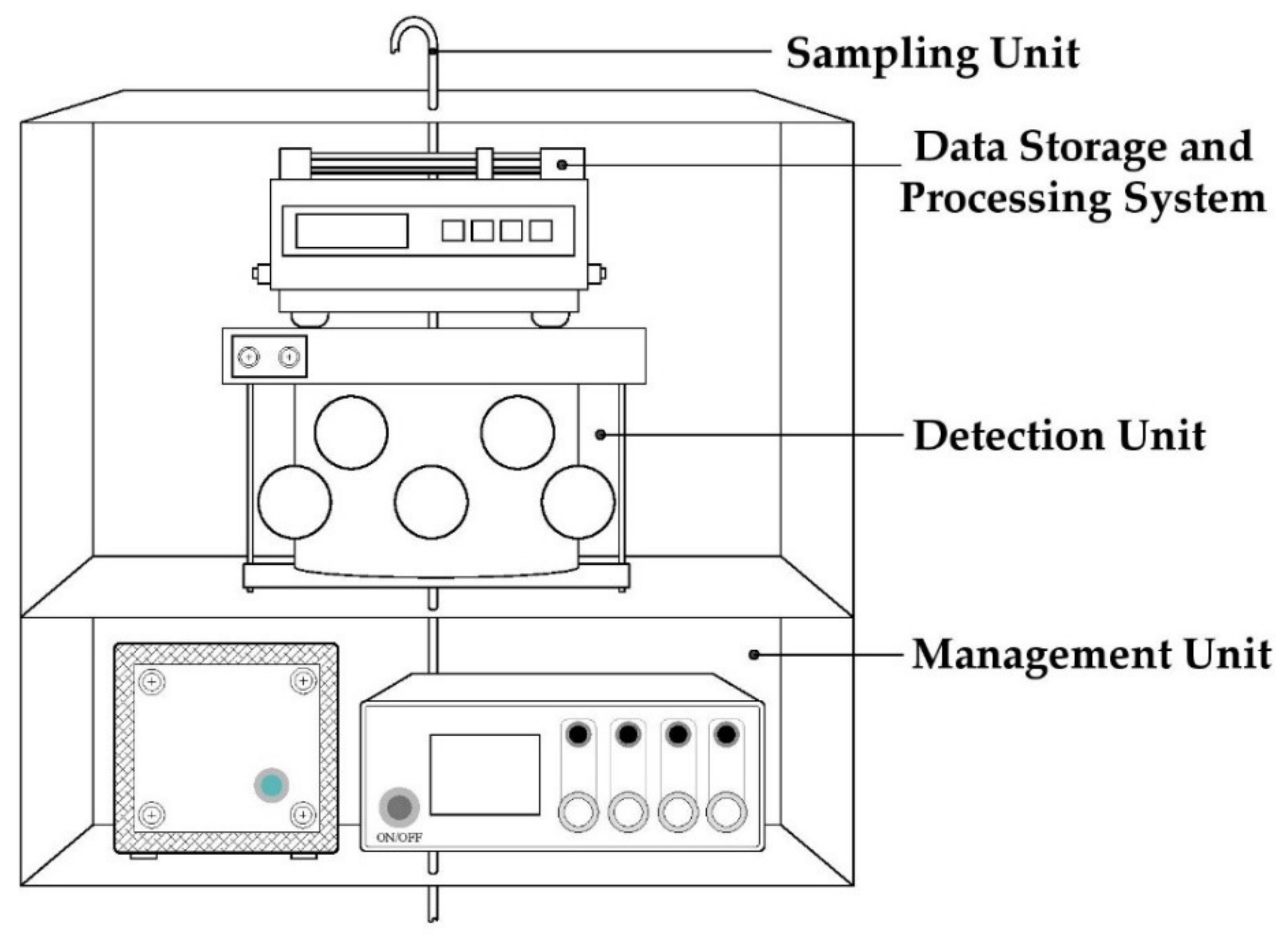
All samples, collected and diluted, were also analysed by an advanced and innovative Instrumental Odour Monitoring System (IOMS), designed by the Sanitary Environmental Engineering Division (SEED) Group of the Department of Civil Engineering of the University of Salerno. The adopted IOMS functional architecture is composed of four principal units: (a) the sampling unit, (b) the detection system, (c) the data storage and processing system and (d) the management unit (Figure 1) [61]. The sampling unit includes a pump for the raw air collection at a flowrate of 300 mL min−1. The detection system incorporates the code (Chamber for Odour Detection) innovative measurement chamber, patented by the SEED research group, in which are located 13 metal oxide semiconductor (MOS) measurement sensors and 3 control sensors [62,63]. The code chamber is cylindrical in shape, with one internal diffuser and the sensors arranged on two levels, each hosting 8 sensors, such as to reproduce the human nasal apparatus consisting of two nostrils and a central nasal septum [63]. Moreover, other subparts include temperature and humidity control and a thermoregulation system, CPU board (Raspberry Pi), HUB i2c board and the main board, particulate and activated carbon filter, ozone cleaning system and permeation tube, pumps and manifold with internal solenoid valves for the different management of gaseous flows, and flexible pipes for the connection between the different components.
The samples were analysed in an “odour–odourless–odour” cycle, with an acquisition and recovery time of 2 min and a time step of 2 s for value. According to Zarra et al. (2021), the peak points (last 1-min interval) have been considered in terms of feature extraction, resulting the most stable and representative [29].
2.3. Odour Quantification Monitoring Models (OQMM) Development
Two different non-parametric (artificial neural network, ANN; multivariate adaptive regression splines, MARSpline) and three parametric (partial least square, PLS; multiple linear regression, MLR; response surface regression, RSR) prediction techniques were investigated and subsequently compared. Each technique has its own unique set of properties. Table 1 presents the indicator considered as index for the OQMM elaboration for each investigated technique [18,51,64,65,66,67,68,69,70,71].
In training the OQMMs and assessing the individual prediction accuracy, supervised learning technique were applied. Applying a k-fold cross-validation procedure (k = 10) to the 92 acquired samples, 82 samples were used as train data sets, while 10 samples were used as validation data sets. To ensure the reliability of the results, the validation data are selected randomly using Microsoft Excel software. Thirty (30) values from each MOS measurement sensor per sample were recorded in the acquisition time, with a frequency of one value every two seconds. The matrix composed of the values detected by the 13 measurement sensors for each sample was then associated with the respective value of the odour concentration measured by dynamic olfactometry. Table 2 summarizes the experimental dataset for the training and validation phase.
2.3.1. ANN
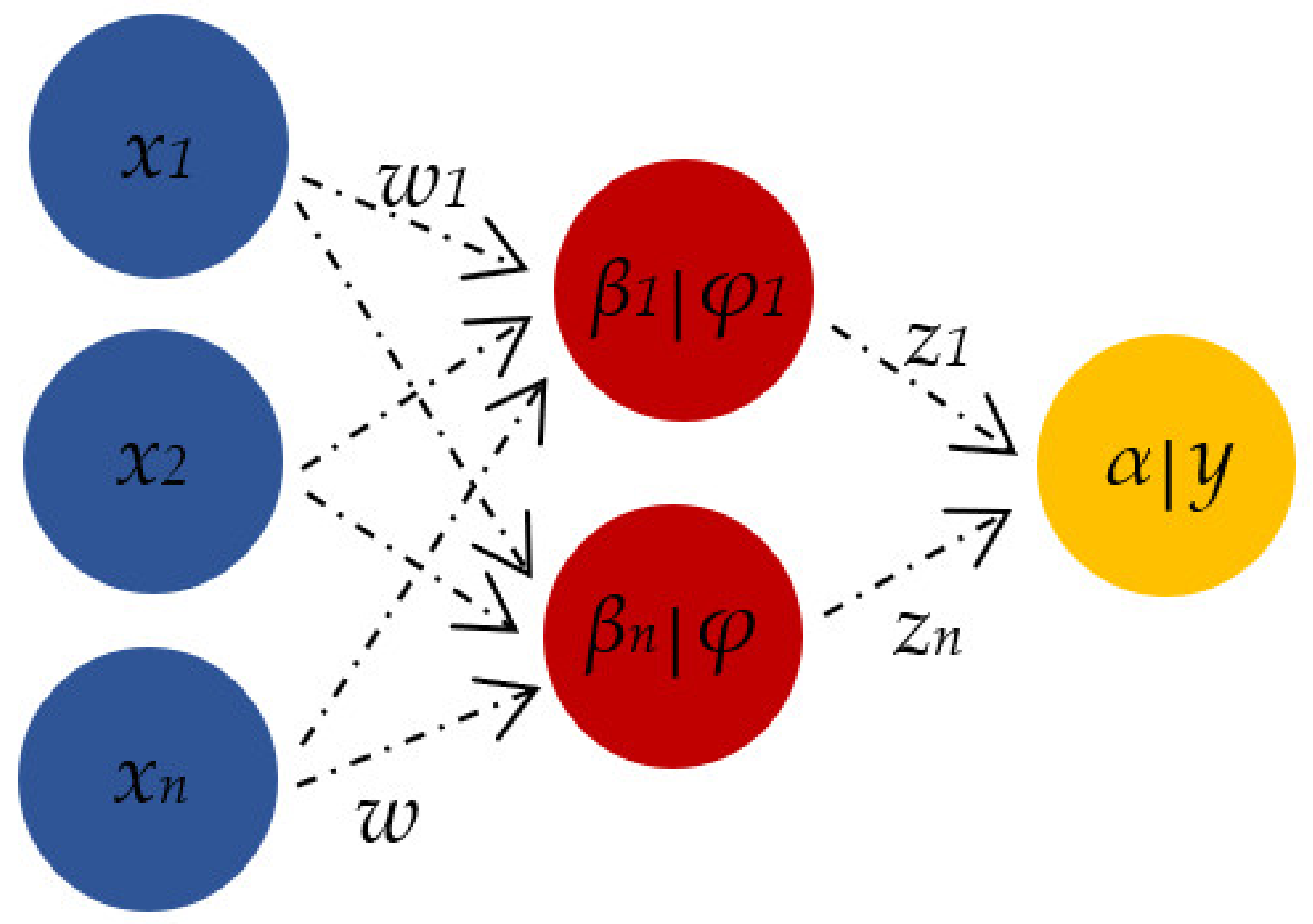
For the ANN experiment, a feed-forward neural network (FFNN) consisting of three layers (input, hidden and output layer) was applied. Tan-sigmoid was used as a neural transfer function, while the network was trained using a Bayesian Regularisation algorithm. The number of neurons in the hidden layer was evaluated between 5–15, in order to avoid underfitting and/or overfitting [15]. In ANN, the input neurons (x) are connected to each other with corresponding weight (w) values. The hidden layer (φ) connects the input variables (x) to the target output variable (y) (Figure 2) [64].
The incoming signal to each neuron was given by the value of the neuron multiplied by the weight, obtaining the total sum from other neurons (Equation (1)), and converting it using the activated function highlighted in the Equations (2) and (3). Meanwhile, the target output variable was computed in the same manner as the neurons in the hidden layers (Equation (4)).
2.3.2. MARSPlines
In the MARSPline experiment, the relationship between dependent and independent variables was established by evaluating the ideal number of basic functions (piecewise linear segments). The “divide and conquer” strategy was applied [72]. The training data (space) were divided into segments, and for each of these a specific regression equation was established at different gradients (slopes). The sum of these individual segments, according to Equation (5), represents the MARSPline model [60]. In the study, each MARSPline model was evaluated starting from 10 basic functions, extracting the coefficients and investigating the most accurate one [51,66].
where:
- -
- β0 = intercept parameter;
- -
- βm = weighted sum of one or more basis functions (hm(X));
- -
- M = sum over the non-constant terms of the model.
2.3.3. MLR
In the MLR experiment, the relationship between the dependent and independent variables was elaborated by implementing a scatter plot, at the centre of the multi-dimensional space of data points, in order to find the collinearity of the variables. The linear equation with the highest correlation (R2) was considered as an optimum MLR model [70]. The Equation (6) highlights an example of a multiple linear regression model, with n predictor variables (x1, x2 … xn) and a response y:
where:
y = β0 + β1 x1 + β2 x2… βnxn + C,
- -
- C = residual terms of the model and the distribution assumption;
- -
- β0, β1, β2… βn = regression coefficients.
2.3.4. PLS
PLS was implemented in an algorithm with simultaneous principal component analysis (PCA) and Ordinary Least Square (OLS) regression. In this experiment, the ideal number of components was evaluated to be between 5–15. PLS reduces the number of input variables to formulate a new set of components that described the maximum correlation between independent and dependent variables. Its prediction ability lies on a set of orthogonal factors, namely component scores or latent variables [44,53]. After selecting the optimal number of components, the loading values and intercepts were extracted to obtain the prediction equation. Equation (7) highlights a PLS regression model with n predictor variables (X1, X2 … X n) and a target output variable y:
where:
y = β0 + β1 X 1 + β2 X 2… βn Xn + C,
- -
- C = residual terms of the model and the distribution assumption;
- -
- β0, β1, β2… βn = weights/coefficients.
2.3.5. RSR
RSR experiments were carried out by investigating the ideal combinations of the independent variables in relation to the target output. In this technique, each of the 13 MOS measurement sensors (as an independent variable) were removed one by one, and the RSR equation at the given number of independent variables was tested. The variable/s with the least influence on the accuracy of the prediction was then determined and eliminated in order to obtain the optimal RSR model. The linear or square polynomial functions were used to define the system, exploring the experimental conditions leading to the optimal situation [67]. The goal was to find the polynomial approximation of the true nonlinear model closest to the Taylor series expansion in the computation. In response surface regression, it contains the similar effects of polynomial regression designs to 2nd degree and 2-way interaction of the variables. It has the characteristics of both polynomial regression designs and fractional factorial regression designs. Equation (8) reports the regression equation for a quadratic response surface regression design.
where:
y = β0 + β1 w + β2 w2 + β3 x + β4 x2+ β5 z + β6 z2 + β7 w x + β8 w z + β9 z z,
- -
- w, x, and z are the predictor variables;
- -
- β0… β9 are the coefficients.
2.4. Statistical Analysis
Statistica 10 (Statsoft, Tulsam, OK, USA), MATLAB R2017a (MathWorks, Natick, MA, USA) and Excel 2013 software (Microsoft, Washington, DC, USA) were applied for data analysis. The individual accuracy of the investigated OQMMs was evaluated based on a coefficient of determination (R2) (Equation (9)) and root mean square error (RMSE) (Equation (10)) analysis.
where:
- -
- , is the sum of squared residuals (SSR);
- -
- , is the sum squared total error (SST),
- -
- x represents the predicted data,
- -
- is the actual data;
- -
- is the mean value of the dataset;
- -
- n is the total number of observations.
The R2 test was used to describe how well the model fits the predicted data. The higher the R2, the more confidence given to the accuracy of the prediction model. Meanwhile, the RMSE value was determined in order to analyse the standard deviation of the residuals (prediction errors).
2.5. Comparison Analysis
The matrix of the different investigated OQMMs is shown in Table 3. The accuracy per OQMM has been evaluated by means of comparing the R2 and RMSE for a training and validation dataset.
3. Results and Discussions
3.1. Odour Concentration Quantification by Dynamic Olfactometry
Figure 3 highlights the statistical characteristics of all of the investigated real odour samples measured by dynamic olfactometry in terms of odour concentration (OUE m−3), using the box and whisker diagram for the overall monitored period.
As shown, the range in terms of odour concentration of the investigated samples is between 81 OUE m−3 (min) and 5793 OUE m−3 (max), covering a wide variability of values both for the representation of emissions and of the emissions scenario. The on-site collected real odorous samples are principally located at the 4th quartile, while the diluted data were at the 1st–3rd quartile. The overall mean, variance and standard deviation is respectively equal to 1695 OUE m−3, 9.70 × 10⁵ and 879 OUE m−3.
3.2. Odour Quantification Monitoring Models (OQMMs)
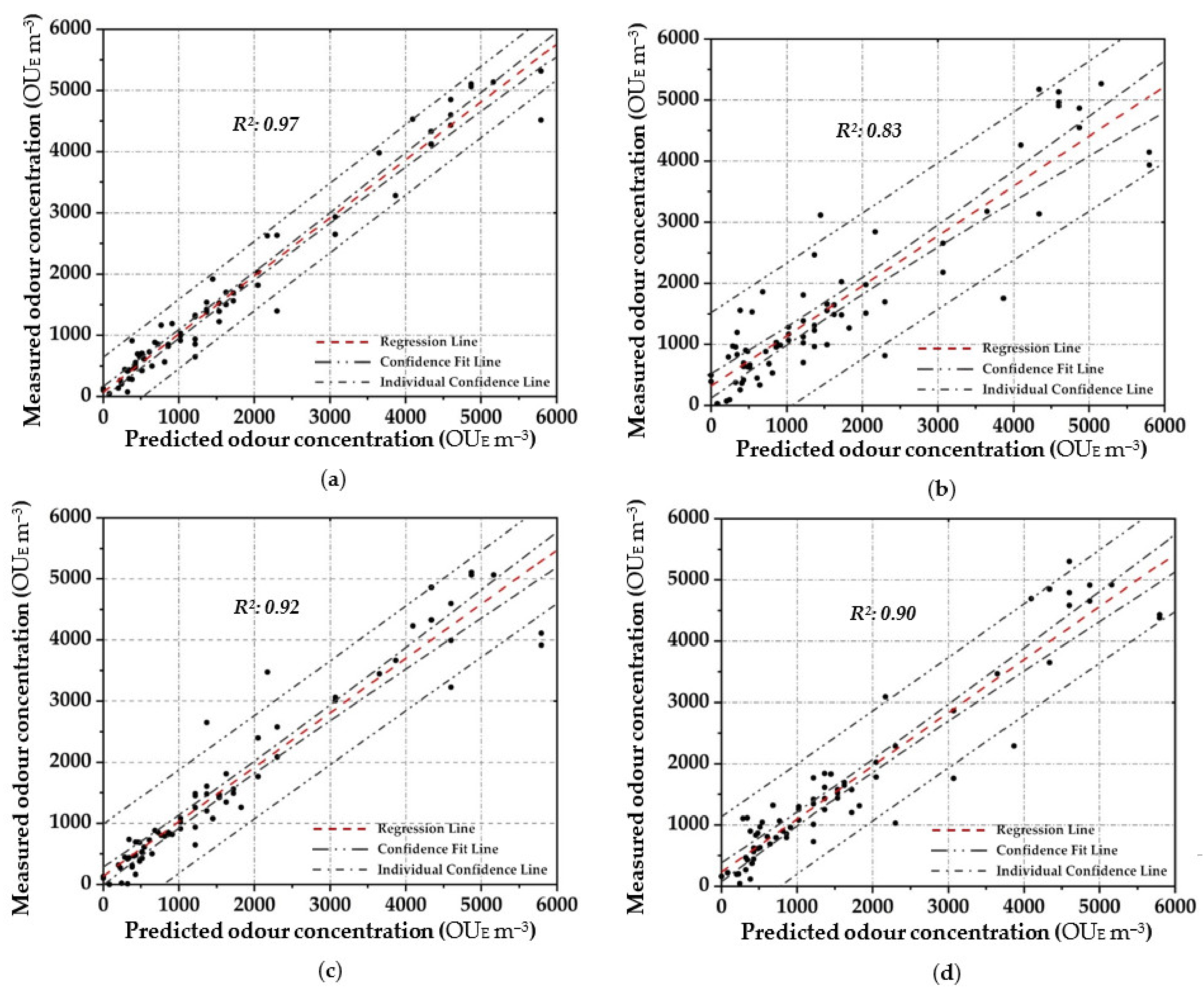
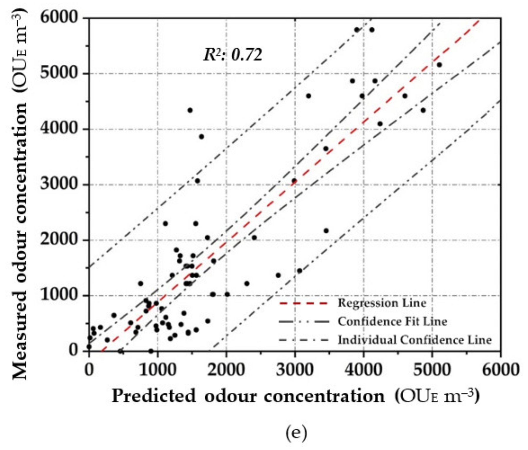
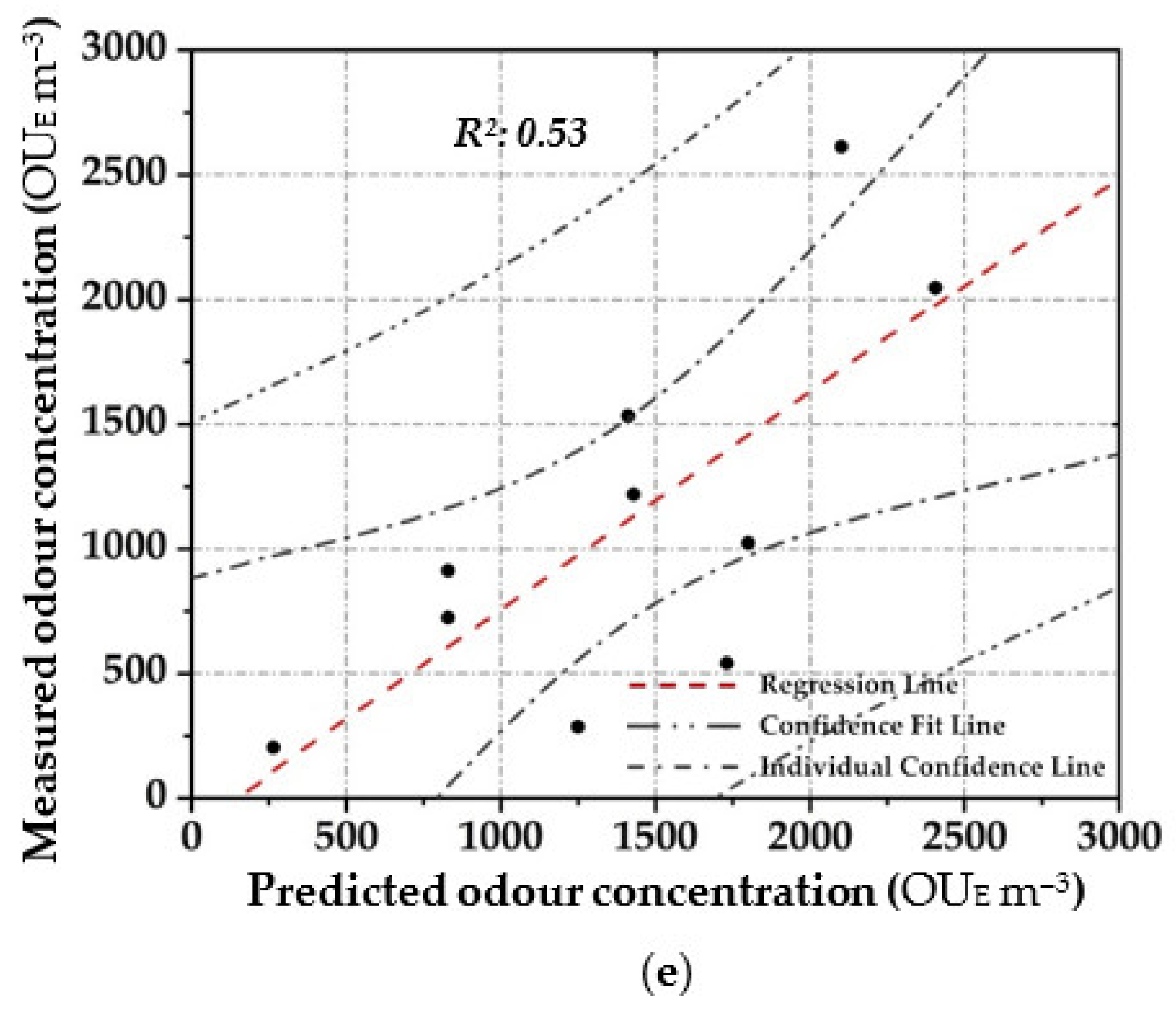
Figure 4 shows the scatter plot diagram between the measured odour concentration with DO, and the predicted values with the elaborated OQMM determined by applying the different parametric and non-parametric prediction techniques, during the training stage. Meanwhile Figure 5 depicts the scatter plot diagram of the relationship by applying the validation dataset. In order to express the certainty of the prediction, a 95% confidence level is applied and presented to all figures.
Applying ANN, a strong pattern relationship between input to output in terms of R2 of 0.97 is highlighted by using the training dataset (Figure 4a); this is depicted by the small number of outliers outside the confidence interval. Similarly, a high correlation (R2: 0.95) is obtained in the validation stage (Figure 5a). For both stages, a percentage of around 80% of the data points are located within the confidence interval. Therefore, the predicted results using ANN are in good agreement with the reference values.
In MARSPline application, results show more spread-out data from the regression line compared to ANN. MARSPLine is ideal when the predictor variables do not exhibit a monotone relationship to the dependent variable of interest [51,72]. According to the “divide and conquer” strategy, the curse of dimensionality from the data has been overcome when the input space is partitioned. The optimum model in the training stage was found at 25 basic functions (R2: 0.83) (Figure 4b). At this point, despite the increase in the number of basic functions, there is a negligible increase in the correlation value; thus, the optimum MARSPline model is taken into account at this extremity. During the validation of the model, the amount of spread in the data is also observed in this stage (R2: 0.87) (Figure 5b).
For the OQMM elaboration by PLS application, results show that the ideal number of components is 10. The accuracy in the training stage, in terms of R2, is defined as equal to 0.92 (Figure 4c). PLS highlights better efficiency when the dataset does not exhibit large variances or noisy information [69]. Furthermore, in the investigated case, a strong correlation at high odour concentrations (>4.00 × 10⁻³ OUE m−3) proves to be difficult to establish. Meanwhile, during the validation stage, PLS accuracy in terms of R2 assumes values comparable to those of ANN (R2: 0.92) (Figure 5c). However, on the basis of the confidence interval, ANN application seems to be more reliable than PLS.
RSR applications were started by testing all of the input/independent variables (e.g., 13 MOS sensors) to ascertain which variable/s may have the least impact to the output. The activity was done to identify prior knowledge of the variable’s interaction. Subsequently, one, or at most two, variables randomly selected were removed, and the consequent accuracy was calculated. For the analysed samples, the highest accuracy was obtained by removing one variable (e.g., one sensor), obtaining at least an R2 equal to 0.90 in the training stage (Figure 4d). Meanwhile, for the validation dataset, a lesser correlation (R2: 0.82) was determined, demonstrating the technique comparable to that of the technique MARSpline (Figure 5d).
3.3. Comparative Analysis
Table 4 summarises and compares the different performances of the investigated OQMMs during training and validation stages, considering the sensors’ responses as input/independent variables, and the odour concentration as output/dependent variable. In particular, the comparison between the performances was carried out by analysing the relative values, given by the difference between those calculated in terms of R2 and/or RMSE, obtained by adopting the different prediction techniques. In fact, it should be noted that the calculated R2 data, in absolute value, could be influenced by the potential reaction between the constituent substances of the samples [69].
Among the parametric prediction techniques, the data reported in Table 4 show how the application of PLS leads to the highest performance. This result is probably due to the ability of PLS to reduce dimensions by transforming and compressing the independent variables into a few components as new inputs, which makes the computation faster. While using the RSR, the obtained performance, in comparison to the other investigated techniques, was lower, especially by applying the validation dataset. RSR can be a tool to analyse the sensitivity of input variables with respect to their relevance to the target output. On the other hand, MLR has been shown to be the most sensitive to outliers. MLR does not appear to achieve satisfactory levels of performance.
While between the non-parametric prediction techniques, ANN highlighted the best performance. ANN shows a stronger capability to map non-linear pattern connection between the input variables to the target output. ANN is more accurate because MARSPLine still ensembles linear function in segmented ways. However, architecting ANN is a challenging task, because of numerous configurations required thorough investigation and knowledge (i.e., number of neurons in the hidden layer, appropriate training algorithm, proper activation function, etc.). Overall, from a prediction accuracy point of view, ANN provides the best results in terms of the high R2 and low RMSE.
As reported, the results refer to the analysis of odour concentrations carried out using the dynamic olfactometry as a reference method, in accordance with EN13725: 2003 for the samples collected at the emission, and the dilution method for these representatives of the conditions detectable at the receptors level.
4. Conclusions
The Instrumental Odour Monitoring System (IOMS) is a useful tool to continuously monitor odour emissions from a municipal solid waste treatment plant, and to control their potential negative impacts on the surrounding area in terms of the predicted OUE m−3. Thus, the elaboration of OQMM is necessary, by using parametric or non-parametric mathematical prediction techniques. Among the investigated techniques, ANN (parametric technique) highlighted the best performance on the basis of R2 and RMSE, while MLR (non-parametric technique) was the lowest.
This study shows how the choice of the prediction technique affects the accuracy in terms of environmental odour concentration prediction of an IOMS. This way, the production of flexible IOMSs that can easily implement different statistical models is suggested, in order to analyse and identify the best performing model for the specific case to be analysed.
Author Contributions
Conceptualization, T.Z. and M.G.K.G.; methodology, T.Z. and M.G.K.G.; software, M.G.K.G.; validation, V.B., V.N., T.Z.; formal analysis, T.Z. and M.G.K.G.; investigation, T.Z., M.G.K.G. and V.N.; resources, V.B., V.N. and T.Z.; data curation, T.Z. and M.G.K.G.; writing—original draft preparation and review and editing T.Z. and M.G.K.G.; supervision, V.N., T.Z. and V.B.; project administration, T.Z.; funding acquisition T.Z. All authors have read and agreed to the published version of the manuscript.
Funding
This research was funded by the University of Salerno, FARB projects: 300393FRB19ZARRA and 300393FRB20ZARRA.
Institutional Review Board Statement
Not applicable.
Informed Consent Statement
Not applicable.
Data Availability Statement
The data presented in this study are available on request from the corresponding author.
Conflicts of Interest
The authors declare no conflict of interest.
References
- Brancher, M.; Griffiths, K.D.; Franco, D.; de Melo Lisboa, H. A review of odour impact criteria in selected countries around the world. Chemosphere 2017, 168, 1531–1570. [Google Scholar] [CrossRef] [PubMed]
- Kerckhoffs, J.; Hoek, G.; Portengen, L.; Brunekreef, B.; Vermeulen, R.C.H. Performance of Prediction Algorithms for Modeling Outdoor Air Pollution Spatial Surfaces. Environ. Sci. Technol. 2019, 53, 1413–1421. [Google Scholar] [CrossRef] [PubMed] [Green Version]
- Kimbrough, S.; Krabbe, S.; Baldauf, R.; Barzyk, T.; Brown, M.; Brown, S.; Croghan, C.; Davis, M.; Deshmukh, P.; Duvall, R.; et al. The Kansas City transportation and local-scale air quality study (KC-TRAQS): Integration of low-cost sensors and reference grade monitoring in a complex metropolitan area. Part 1: Overview of the project. Chemosensors 2019, 7, 26. [Google Scholar] [CrossRef] [Green Version]
- Belgiorno, V.; Naddeo, V.; Zarra, T. Odour Impact Assessment Handbook; John & Wiley Sons, Inc.: Hoboken, NJ, USA, 2012. [Google Scholar]
- Wu, C.; Liu, J.; Liu, S.; Li, W.; Yan, L.; Shu, M.; Zhao, P.; Zhou, P.; Cao, W. Assessment of the health risks and odor concentration of volatile compounds from a municipal solid waste landfill in China. Chemosphere 2018, 202, 1–8. [Google Scholar] [CrossRef]
- Fernández-González, J.M.; Díaz-López, C.; Martín-Pascual, J.; Zamorano, M. Recycling organic fraction of municipal solid waste: Systematic literature review and bibliometric analysis of research trends. Sustainability 2020, 12, 4798. [Google Scholar] [CrossRef]
- Piringer, M.; Schauberger, G. Environmental odour: Emission, dispersion, and the assessment of annoyance. Atmosphere 2020, 11, 896. [Google Scholar] [CrossRef]
- Stafford, L.D.; Fleischman, D.S.; Le Her, N.; Hummel, T. Exploring the emotion of disgust: Differences in smelling and feeling. Chemosensors 2018, 6, 9. [Google Scholar] [CrossRef] [Green Version]
- Chang, H.; Zhao, Y.; Tan, H.; Liu, Y.; Lu, W.; Wang, H. Parameter sensitivity to concentrations and transport distance of odorous compounds from solid waste facilities. Sci. Total Environ. 2019, 651, 2158–2165. [Google Scholar] [CrossRef]
- Han, Z.; Qi, F.; Li, R.; Wang, H.; Sun, D. Health impact of odor from on-situ sewage sludge aerobic composting throughout different seasons and during anaerobic digestion with hydrolysis pretreatment. Chemosphere 2020, 249, 126077. [Google Scholar] [CrossRef]
- Zarra, T.; Giuliani, S.; Naddeo, V.; Belgiorno, V. Control of odour emission in wastewater treatment plants by direct and undirected measurement of odour emission capacity. Water Sci. Technol. 2012, 66, 1627–1633. [Google Scholar] [CrossRef] [Green Version]
- Hettinger, T.P.; Frank, M.E. Stochastic and temporal models of olfactory perception. Chemosensors 2018, 6, 44. [Google Scholar] [CrossRef] [Green Version]
- Tang, X.; Xiao, W.; Shang, T.; Zhang, S.; Han, X.; Wang, Y.; Sun, H. An electronic nose technology to quantify pyrethroid pesticide contamination in tea. Chemosensors 2020, 8, 30. [Google Scholar] [CrossRef]
- Wilson, A.D. Applications of electronic-nose technologies for noninvasive early detection of plant, animal and human diseases. Chemosensors 2018, 6, 45. [Google Scholar] [CrossRef] [Green Version]
- Zarra, T.; Galang, M.G.; Ballesteros, F.; Belgiorno, V.; Naddeo, V. Environmental odour management by artificial neural network—A review. Environ. Int. 2019, 133, 105189. [Google Scholar] [CrossRef]
- Fasolino, I.; Grimaldi, M.; Zarra, T.; Naddeo, V. Odour control strategies for a sustainable nuisances action plan. Glob. Nest J. 2016, 18, 734–741. [Google Scholar] [CrossRef] [Green Version]
- Zarra, T.; Reiser, M.; Naddeo, V.; Belgiorno, V.; Kranert, M. Odour Emissions Characterization from Wastewater Treatment Plants by Different Measurement Methods. Chem. Eng. Trans. 2014, 40, 37–42. [Google Scholar] [CrossRef]
- Galang, M.G.K.; Zarra, T.; Naddeo, V.; Belgiorno, V.; Ballesteros, F. Artificial neural network in the measurement of environmental odours by e-nose. Chem. Eng. Trans. 2018, 68, 247–252. [Google Scholar] [CrossRef]
- Laor, Y.; Parker, D.; Pagé, T. Measurement, prediction, and monitoring of odors in the environment: A critical review. Rev. Chem. Eng. 2014, 30, 139–166. [Google Scholar] [CrossRef]
- Oliva, G.; Zarra, T.; Pittoni, G.; Senatore, V.; Galang, M.G.; Castellani, M.; Belgiorno, V.; Naddeo, V. Next-generation of instrumental odour monitoring system (IOMS) for the gaseous emissions control in complex industrial plants. Chemosphere 2021, 271, 129768. [Google Scholar] [CrossRef]
- Gobbi, E.; Falasconi, M.; Zambotti, G.; Sberveglieri, V.; Pulvirenti, A.; Sberveglieri, G. Rapid diagnosis of Enterobacteriaceae in vegetable soups by a metal oxide sensor based electronic nose. Sens. Actuators B Chem. 2015, 207, 1104–1113. [Google Scholar] [CrossRef]
- Abdulrazzaq, N.N.; Al-Sabbagh, B.H.; Rees, J.M.; Zimmerman, W.B. Measuring vapor and liquid concentrations for binary and ternary systems in a microbubble distillation unit via gas sensors. Chemosensors 2018, 6, 31. [Google Scholar] [CrossRef] [Green Version]
- Guillot, J.M. E-noses: Actual limitations and perspectives for environmental odour analysis. Chem. Eng. Trans. 2016, 54, 223–228. [Google Scholar] [CrossRef]
- Naddeo, V.; Zarra, T.; Oliva, G.; Kubo, A.; Ukida, N.; Higuchi, T. Odour measurement in wastewater treatment plant by a new prototype of e.nose: Correlation and comparison study with reference to both European and Japanese approaches. Chem. Eng. Trans. 2016, 54, 85–90. [Google Scholar]
- Conti, C.; Guarino, M.; Bacenetti, J. Measurements techniques and models to assess odor annoyance: A review. Environ. Int. 2020, 134, 105261. [Google Scholar] [CrossRef] [PubMed]
- Szulczyński, B.; Gębicki, J. Electronic nose—An instrument for odour nuisances monitoring. E3S Web Conf. 2019, 100. [Google Scholar] [CrossRef] [Green Version]
- Martinelli, E.; Magna, G.; Polese, D.; Vergara, A.; Schild, D.; Di Natale, C. Stable odor recognition by a neuro-adaptive electronic nose. Sci. Rep. 2015, 5, 1–9. [Google Scholar] [CrossRef] [PubMed] [Green Version]
- Pelosi, P.; Zhu, J.; Knoll, W. From gas sensors to biomimetic artificial noses. Chemosensors 2018, 6, 32. [Google Scholar] [CrossRef] [Green Version]
- Zarra, T.; Galang, M.G.K.; Ballesteros, F.C.; Belgiorno, V.; Naddeo, V. Instrumental odour monitoring system classification performance optimization by analysis of different pattern-recognition and feature extraction techniques. Sensors 2021, 21, 114. [Google Scholar] [CrossRef] [PubMed]
- Naddeo, V.; Zarra, T.; Giuliani, S.; Belgiorno, V. Odour impact assessment in industrial areas. Chem. Eng. Trans. 2012, 30, 85–90. [Google Scholar] [CrossRef]
- Gardner, J.W.; Bartlett, P.N. A brief history of electronic noses. Sensors Actuators B Chem. 1994, 18, 210–211. [Google Scholar] [CrossRef]
- Hidayat, S.N.; Triyana, K.; Fauzan, I.; Julian, T.; Lelono, D.; Yusuf, Y.; Ngadiman, N.; Veloso, A.C.A.; Peres, A.M. The electronic nose coupled with chemometric tools for discriminating the quality of black tea samples in situ. Chemosensors 2019, 7, 29. [Google Scholar] [CrossRef] [Green Version]
- Rasekh, M.; Karami, H.; Wilson, A.D.; Gancarz, M. Classification and Identification of Essential Oils from Herbs and Fruits Based on a MOS Electronic-Nose Technology. Chemosensors 2021, 9, 142. [Google Scholar] [CrossRef]
- Gancarz, M.; Malaga-Toboła, U.; Oniszczuk, A.; Tabor, S.; Oniszczuk, T.; Gawrysiak-Witulska, M.; Rusinek, R. Detection and measurement of aroma compounds with the electronic nose and a novel method for MOS sensor signal analysis during the wheat bread making process. Food Bioprod. Process. 2021, 127, 90–98. [Google Scholar] [CrossRef]
- Kwiatkowski, A.; Chludziński, T.; Saidi, T.; Welearegay, T.G.; Jaimes-Mogollón, A.L.; El Bari, N.; Borys, S.; Bouchikhi, B.; Smulko, J.; Ionescu, R. Assessment of electronic sensing techniques for the rapid identification of alveolar echinococcosis through exhaled breath analysis. Sensors 2020, 20, 2666. [Google Scholar] [CrossRef] [PubMed]
- Khan, S.; Le Calvé, S.; Newport, D. A review of optical interferometry techniques for VOC detection. Sens. Actuators A Phys. 2020, 302. [Google Scholar] [CrossRef]
- Kabir, E.; Raza, N.; Kumar, V.; Singh, J.; Tsang, Y.F.; Lim, D.K.; Szulejko, J.E.; Kim, K.H. Recent Advances in Nanomaterial-Based Human Breath Analytical Technology for Clinical Diagnosis and the Way Forward. Chem 2019, 5, 3020–3057. [Google Scholar] [CrossRef]
- Sethi, S.; Nanda, R.; Chakraborty, T. Clinical application of volatile organic compound analysis for detecting infectious diseases. Clin. Microbiol. Rev. 2013, 26, 462–475. [Google Scholar] [CrossRef] [Green Version]
- Slimani, S.; Bultel, E.; Cubizolle, T.; Herrier, C.; Rousselle, T.; Livache, T. Opto-electronic nose coupled to a silicon micro pre-concentrator device for selective sensing of flavored waters. Chemosensors 2020, 8, 60. [Google Scholar] [CrossRef]
- Yurko, G.; Roostaei, J.; Dittrich, T.; Xu, L.; Ewing, M.; Zhang, Y.; Shreve, G. Real-Time Sensor Response Characteristics of 3 Commercial Metal Oxide Sensors for Detection of BTEX and Chlorinated Aliphatic Hydrocarbon Organic Vapors. Chemosensors 2019, 7, 40. [Google Scholar] [CrossRef] [Green Version]
- Korsa, M.T.; Domingo, J.M.C.; Nsubuga, L.; Hvam, J.; Niekiel, F.; Lofink, F.; Rubahn, H.G.; Adam, J.; Hansen, R.D.O. Optimizing piezoelectric cantilever design for electronic nose applications. Chemosensors 2020, 8, 114. [Google Scholar] [CrossRef]
- Cao, J.; Liu, T.; Chen, J.; Yang, T.; Zhu, X.; Wang, H. Drift Compensation on Massive Online Electronic-Nose Responses. Chemosensors 2021, 9, 78. [Google Scholar] [CrossRef]
- Licen, S.; Barbieri, G.; Fabbris, A.; Briguglio, S.C.; Pillon, A.; Stel, F.; Barbieri, P. Odor control map: Self organizing map built from electronic nose signals and integrated by different instrumental and sensorial data to obtain an assessment tool for real environmental scenarios. Sens. Actuators B Chem. 2018, 263, 476–485. [Google Scholar] [CrossRef]
- Abdi, H. Partial least squares regression and projection on latent structure regression (PLS Regression). Wiley Interdiscip. Rev. Comput. Stat. 2010, 2, 97–106. [Google Scholar] [CrossRef]
- Distante, C.; Leo, M.; Siciliano, P.; Persaud, K.C. On the study of feature extraction methods for an electronic nose. Sens. Actuators B Chem. 2002, 87, 274–288. [Google Scholar] [CrossRef]
- Teniou, A.; Rhouati, A.; Marty, J.L. Mathematical Modelling of Biosensing Platforms Applied for Environmental Monitoring. Chemosensors 2021, 9, 50. [Google Scholar] [CrossRef]
- Abbatangelo, M.; Núñez-Carmona, E.; Sberveglieri, V.; Comini, E.; Sberveglieri, G. k-NN and k-NN-ANN combined classifier to assess mox gas sensors performances affected by drift caused by early life aging. Chemosensors 2020, 8, 6. [Google Scholar] [CrossRef] [Green Version]
- Ding, S.; Zhu, H.; Jia, W.; Su, C. A survey on feature extraction for pattern recognition. Artif. Intell. Rev. 2012, 37, 169–180. [Google Scholar] [CrossRef]
- Okur, S.; Sarheed, M.; Huber, R.; Zhang, Z.; Heinke, L.; Kanbar, A.; Wöll, C.; Nick, P.; Lemmer, U. Identification of Mint Scents Using a QCM Based E-Nose. Chemosensors 2021, 9, 31. [Google Scholar] [CrossRef]
- Szulczyński, B.; Armiński, K.; Namieśnik, J.; Gębicki, J. Determination of odour interactions in gaseous mixtures using electronic nose methods with artificial neural networks. Sensors 2018, 18, 519. [Google Scholar] [CrossRef] [Green Version]
- Lokuge, W.; Wilson, A.; Gunasekara, C.; Law, D.W.; Setunge, S. Design of fly ash geopolymer concrete mix proportions using Multivariate Adaptive Regression Spline model. Constr. Build. Mater. 2018, 166, 472–481. [Google Scholar] [CrossRef]
- Ojha, P.K.; Roy, K. PLS regression-based chemometric modeling of odorant properties of diverse chemical constituents of black tea and coffee. RSC Adv. 2018, 8, 2293–2304. [Google Scholar] [CrossRef] [Green Version]
- Dahlén, J.; Karlsson, S.; Bäckström, M.; Hagberg, J.; Pettersson, H. Determination of nitrate and other water quality parameters in groundwater from UV/Vis spectra employing partial least squares regression. Chemosphere 2000, 40, 71–77. [Google Scholar] [CrossRef]
- Zhang, C.; Wang, W.; Pan, Y. Enhancing electronic nose performance by feature selection using an improved grey wolf optimization based algorithm. Sensors 2020, 20, 4065. [Google Scholar] [CrossRef] [PubMed]
- Hansen, M.J.; Jonassen, K.E.N.; Løkke, M.M.; Adamsen, A.P.S.; Feilberg, A. Multivariate prediction of odor from pig production based on in-situ measurement of odorants. Atmos. Environ. 2016, 135, 50–58. [Google Scholar] [CrossRef]
- Orzi, V.; Riva, C.; Scaglia, B.; D’Imporzano, G.; Tambone, F.; Adani, F. Anaerobic digestion coupled with digestate injection reduced odour emissions from soil during manure distribution. Sci. Total Environ. 2018, 621, 168–176. [Google Scholar] [CrossRef]
- Matias-Guiu, P.; Garza-Moreira, E.; Rodríguez-Bencomo, J.J.; López, F. Rapid sensory analysis using response surface methodology: Application to the study of odour interactive effects in model spirits. J. Inst. Brew. 2018, 124, 100–105. [Google Scholar] [CrossRef] [Green Version]
- Keller, A.; Gerkin, R.C.; Guan, Y.; Dhurandhar, A.; Turu, G.; Szalai, B.; Mainland, J.D.; Ihara, Y.; Yu, C.W.; Wolfinger, R.; et al. Predicting human olfactory perception from chemical features of odor molecules. Science 2017, 355, 820–826. [Google Scholar] [CrossRef] [PubMed] [Green Version]
- Geană, E.I.; Ciucure, C.T.; Apetrei, C. Electrochemical sensors coupled with multivariate statistical analysis as screening tools for wine authentication issues: A review. Chemosensors 2020, 8, 59. [Google Scholar] [CrossRef]
- Zhang, W.; Goh, A.T.C. Multivariate adaptive regression splines and neural network models for prediction of pile drivability. Geosci. Front. 2016, 7, 45–52. [Google Scholar] [CrossRef] [Green Version]
- Giuliani, S.; Zarra, T.; Nicolas, J.; Naddeo, V.; Belgiorno, V.; Romain, A.C. An alternative approach of the e-nose training phase in odour impact assessment. Chem. Eng. Trans. 2012, 30, 139–144. [Google Scholar] [CrossRef]
- Giuliani, S.; Zarra, T.; Naddeo, V.; Belgiorno, V. Measurement of odour emission capacity in wastewater treatment plants by multisensor array system. Environ. Eng. Manag. J. 2013, 12, 173–176. [Google Scholar]
- Viccione, G.; Zarra, T.; Giuliani, S.; Naddeo, V.; Belgiorno, V. Performance study of e-nose measurement chamber for environmental odour monitoring. Chem. Eng. Trans. 2012, 30, 109–114. [Google Scholar] [CrossRef]
- Galang, M.G.K.; Ballesteros, F. Estimation of waste mobile phones in the Philippines using neural networks. Glob. Nest J. 2018, 20, 767–772. [Google Scholar] [CrossRef] [Green Version]
- Khaldi, S.; Dibi, Z. Neural Network Technique for Electronic Nose Based on High Sensitivity Sensors Array. Sens. Imaging 2019, 20, 1–19. [Google Scholar] [CrossRef]
- Oduro, S.D.; Metia, S.; Duc, H.; Hong, G.; Ha, Q.P. Multivariate adaptive regression splines models for vehicular emission prediction. Vis. Eng. 2015, 3. [Google Scholar] [CrossRef] [Green Version]
- Bezerra, M.A.; Santelli, R.E.; Oliveira, E.P.; Villar, L.S.; Escaleira, L.A. Response surface methodology (RSM) as a tool for optimization in analytical chemistry. Talanta 2008, 76, 965–977. [Google Scholar] [CrossRef]
- Vedrtnam, A.; Singh, G.; Kumar, A. Optimizing submerged arc welding using response surface methodology, regression analysis, and genetic algorithm. Def. Technol. 2018, 14, 204–212. [Google Scholar] [CrossRef]
- Wang, H.; Gu, J.; Wang, S.; Saporta, G. Spatial partial least squares autoregression: Algorithm and applications. Chemom. Intell. Lab. Syst. 2019, 184, 123–131. [Google Scholar] [CrossRef]
- Al-Salem, S.M.; Al-Nasser, A.; Al-Dhafeeri, A.T. Multi-variable regression analysis for the solid waste generation in the State of Kuwait. Process. Saf. Environ. Prot. 2018, 119, 172–180. [Google Scholar] [CrossRef]
- Kang, J.H.; Song, J.H.; Yoo, S.S.; Lee, B.J.; Ji, H.W. Prediction of odor concentration emitted from wastewater treatment plant using an artificial neural network (ANN). Atmosphere 2020, 11, 784. [Google Scholar] [CrossRef]
- Samadi, M.; Afshar, M.H.; Jabbari, E.; Sarkardeh, H. Application of Multivariate Adaptive Regression Splines and Classification and Regression Trees to Estimate Wave-Induced Scour Depth around Pile Groups. Iran. J. Sci. Technol. Trans. Civ. Eng. 2020, 44, 447–459. [Google Scholar] [CrossRef]
Figure 1.
Main functional units of the used Instrumental Odour Monitoring System (IOMS).

Figure 2.
Relationship of neural network elements (x—input neurons, φ—hidden neurons, y—output neuron).
Figure 2.
Relationship of neural network elements (x—input neurons, φ—hidden neurons, y—output neuron).

Figure 3.
Boxplot of the odour concentration of the investigated samples.

Figure 4.
Scatter plot between the measured odour concentration with DO and the predicted one with the elaborated OQMMs using Table 4. ((a)—ANN, (b)—MARSPline, (c)—PLS, (d)—RSR and (e)—MLR).
Figure 4.
Scatter plot between the measured odour concentration with DO and the predicted one with the elaborated OQMMs using Table 4. ((a)—ANN, (b)—MARSPline, (c)—PLS, (d)—RSR and (e)—MLR).


Figure 5.
Scatter plot between the measured odour concentration with DO and the predicted one with the elaborated OQMMs using the different investigated prediction techniques and the validation dataset ((a)—ANN, (b)—MARSPline, (c)—PLS, (d)—RSR and (e)—MLR)).
Figure 5.
Scatter plot between the measured odour concentration with DO and the predicted one with the elaborated OQMMs using the different investigated prediction techniques and the validation dataset ((a)—ANN, (b)—MARSPline, (c)—PLS, (d)—RSR and (e)—MLR)).


Table 1.
Prediction techniques evaluation indicators for the OQMM elaboration.
| Statistical Category | Prediction Technique | Indicators |
|---|---|---|
| Parametric | Multiple Linear Regression (MLR) | Dependent–independent variable relationship |
| Partial Least Square (PLS) | Ideal number of components | |
| Response Surface Regression (RSR) | Significant variables | |
| Non-parametric | Multivariate Adaptive Regression Splines (MARSpline) | Ideal number of basic functions |
| Artificial Neural Network (ANN) | Ideal number of hidden neurons |
Table 2.
Size of the experimental dataset for each of the 13 MOS measurement sensors.
| Description | Number of Observation Points | ||||
|---|---|---|---|---|---|
| Training Dataset | Validation Dataset | OUE m−3 | |||
| Raw Samples | Data Points (kΩ) | Raw Samples | Data Points (kΩ) | ||
| Odorous Air | 82 | 2460 | 10 | 300 | 82 |
Table 3.
Matrix of the different elaborated and compared OQMMs.
| Statistical Category | Prediction Technique | OQMM | |||
|---|---|---|---|---|---|
| Training | Validation | ||||
| R2 | RMSE (OUE m−3) | R2 | RMSE (OUE m−3) | ||
| Parametric | PLS | OQMM1.1 | OQMM2.1 | ||
| RSR | OQMM1.2 | OQMM2.2 | |||
| MLR | OQMM1.3 | OQMM2.3 | |||
| Non-Parametric | ANN | OQMM1.4 | OQMM2.4 | ||
| MARSPline | OQMM1.5 | OQMM2.5 | |||
Table 4.
Summary of the quality parameters of the developed model during training and validation.
| Statistical Category | Prediction Technique for OQMM Elaboration | Training | Validation | ||
|---|---|---|---|---|---|
| R2 | RMSE (OUE m−3) | R2 | RMSE (OUE m−3) | ||
| Parametric | PLS | 0.92 | 451 | 0.92 | 219 |
| RSR | 0.90 | 487 | 0.82 | 348 | |
| MLR | 0.72 | 837 | 0.53 | 583 | |
| Non-Parametric | ANN | 0.97 | 289 | 0.95 | 216 |
| MARSPline | 0.83 | 651 | 0.87 | 482 | |
Publisher’s Note: MDPI stays neutral with regard to jurisdictional claims in published maps and institutional affiliations. |
© 2021 by the authors. Licensee MDPI, Basel, Switzerland. This article is an open access article distributed under the terms and conditions of the Creative Commons Attribution (CC BY) license (https://creativecommons.org/licenses/by/4.0/).
Share and Cite
MDPI and ACS Style
Zarra, T.; Galang, M.G.K.; Belgiorno, V.; Naddeo, V. Environmental Odour Quantification by IOMS: Parametric vs. Non-Parametric Prediction Techniques. Chemosensors 2021, 9, 183. https://0-doi-org.brum.beds.ac.uk/10.3390/chemosensors9070183
AMA Style
Zarra T, Galang MGK, Belgiorno V, Naddeo V. Environmental Odour Quantification by IOMS: Parametric vs. Non-Parametric Prediction Techniques. Chemosensors. 2021; 9(7):183. https://0-doi-org.brum.beds.ac.uk/10.3390/chemosensors9070183
Chicago/Turabian StyleZarra, Tiziano, Mark Gino K. Galang, Vincenzo Belgiorno, and Vincenzo Naddeo. 2021. "Environmental Odour Quantification by IOMS: Parametric vs. Non-Parametric Prediction Techniques" Chemosensors 9, no. 7: 183. https://0-doi-org.brum.beds.ac.uk/10.3390/chemosensors9070183
Note that from the first issue of 2016, this journal uses article numbers instead of page numbers. See further details here.