Pricing Longevity Bonds under a Credibility Framework with Limited Available Data

Abstract

For annuity providers, a higher life expectancy is not always positive news, as it potentially implies increased future costs, since benefits must be provided over a longer period of time. The underlying risk behind the unexpected improvement in life expectancy is called longevity risk. One way to hedge this risk can be attained with the process of securitization through mortality risk securities. This process requires an accurate prediction of the future mortality dynamics with an appropriate mortality model. However, a major issue in mortality modeling is the limited number of available data for a given population. The purpose of this paper is to present a mortality model under the credibility regression framework, aiming to capture the future mortality trends, especially for population datasets of limited available observations. Then, we show how this approach can be incorporated into pricing longevity bonds with the Wang transform. To ensure transparency and applicability in our illustration, the longevity bond pricing is based on the mortality data of Greece.

1. Introduction

The insurance industry related to life insurance and pension plans is facing a number of risks. Longevity risk is one of the most important risks faced by annuity providers, in which participants are promised a benefit throughout their retirement. When people live longer than expected, an increase in longevity risk is observed. Although most of the international demographic trends indicate a steady increase in life expectancy, there are other schools of thought that argue for potential opposite trends due to unknown diseases or other medical reasons (e.g., malnutrition, obesity, etc.).

Despite the fears that these reasons would reverse these trends, life expectancy in developed countries has grown steadily, by approximately 2.5 years per decade. Kisser et al. (2012) show that an increase in life expectancy by one year in the USA raises pension liabilities by 3% to 4%, which is a substantial economic magnitude. Jones (2013) explains how longevity risk can affect most in the whole of society—for example, the governments who have to provide retirement benefits to individuals through pensions and healthcare, the corporate sponsors who provide retirement benefits and health insurance obligations to former employees and individuals who do not rely on governments or corporate sponsors to fund retirement.

In this spirit, actuaries seek solutions through the development of some financial instruments that can offer tools against longevity risk. Traditionally, reinsurance can serve as a hedging tool but sometimes is rather expensive. Securitization can substitute classic reinsurance by transferring risk to third parties. Blake and Burrows (2001) suggested the use of longevity bonds, issued by the governments, with coupon payments proportional to the population surviving to particular ages. The annuity providers would then make payments for a longer period if annuitants lived longer, but in that case, they would also receive a greater offsetting coupon payment on their survivor bonds asset positions. For a further discussion on the securitization process, we refer to Cowley and Cummins (2005).

There is rich literature with various papers on managing longevity risk, including securitization or other hedging techniques. Among others, Lin and Cox (2005) made a remarkable contribution that highlights the main aspects of longevity risk securitization. In their paper, the authors illustrate how insurers can use mortality-based securities to manage longevity risk. They argue that mortality-based securitization has the same structure as the catastrophe risk bonds, but differs in the way that deviations in mortality forecasts may occur gradually over a long period. Moreover, Blake et al. (2006) examined various ways in which an insurer can manage longevity risk, focusing on the use of mortality-linked securities to manage their exposure.

Thomsen and Andersen (2007) observed an imbalance between supply and demand for longevity products explained by the fact that many insurers are interested in hedging their longevity risks, in the absence of investors who want to benefit from an unexpected rise in mortality. Nevertheless, Hari et al. (2008) analyzed the importance of longevity risk for the solvency of annuity portfolios, and focused on the risk that results from uncertainty in the remaining lifetime of a member of a pension plan. They also distinguish two types of longevity risk, the micro-longevity risk that results from non-systematic deviations from a member’s expected remaining lifetime, and the macro-longevity risk that is due to the change in survival probabilities over time.

Furthermore, Yang and Huang (2009) investigated the interplay between asset allocation and longevity risk for defined contribution pension plans, while Barrieu et al. (2012) explored the key risk management challenges for both financial and insurance industries. To make the longevity risk market operational in an efficient and transparent way, De Jong and Ferris (2019) and Lin et al. (2022) proposed the so-called survival–mortality bond, which is a long-term conventional government bond that incorporates a survivorship part and a mortality part. For an extensive review on recent developments related to longevity risk and capital markets, we refer to Blake and Cairns (2021).

An essential step in the process of longevity risk securitization is the selection of the mortality projection model. An appropriate mortality model must be able to handle the mortality patterns of the given data and produce reliable forecasts for building projected life tables. Different modeling approaches have been developed so far. Lin and Cox (2005) used the model of Renshaw et al. (1996) to predict the future mortality improvements needed to price longevity risk securities for US data. One of the most prominent modeling approaches is also the Lee and Carter (1992) model, which is widely used by many researchers. Denuit et al. (2007) applied the original Lee–Carter model on Belgian mortality data in order to price a longevity bond; Levantesi et al. (2008) used the Brouhns et al. (2002) extension of the Lee–Carter model in a similar study for the Italian population, while Kim and Choi (2011) and Lorson and Wagner (2014) priced a longevity bond using the mortality projections of the Lee–Carter model for German and Australian data, respectively.

A critical issue that may appear when fitting a mortality model is the limited data availability, which may affect the existing modeling methods that inevitably base their forecasts on population datasets of limited periods of observations. This paper contributes to the literature in two ways. Firstly, it incorporates a recently developed modeling framework, particularly designed to project mortality rates for datasets, with limited experience for the mortality evolution of a specific age, but extensive experience for the entire fitted range of ages. Secondly, our projected life tables are used to price a longevity bond with the Wang transform for the mortality data of Greece, a country with limited publicly available data.

The remainder of this paper is organized as follows. Section 2 presents the mortality modeling approach under the credibility regression framework with three extrapolation methods to construct projected life tables. Section 3 describes the mathematical structure and the necessary transactions for pricing longevity bonds with the Wang transform. Section 4 applies the whole pricing process to Greek data, and Section 5 concludes the paper.

2. Mortality Projection under the Credibility Regression Framework

In this section, we review the credibility regression mortality framework, presented as a special case of a more general model in Bozikas and Pitselis (2019). Credibility theory includes various estimation techniques, traditionally used in non-life insurance. More specifically, credibility regression was introduced by Hachemeister (1975) to estimate the trend in automobile bodily injury claims for various states in the USA.

Over the last century, empirical mortality data have shown a downward trend in each age. Particularly in higher ages, mortality rates have been significantly improving over the last few decades due to many factors, such as the dynamics of the human race, the improvement of living conditions, medical advances, etc. This fact led us to seek a model structure that will be able to capture these improvement trends and describe the mortality evolution over time, even if our available data are of a limited size. The credibility regression framework will be used to construct projected life tables for datasets with limited experience for the mortality evolution of a specific age, but extensive experience for the entire fitted age range.

2.1. Notation and Assumptions

We denote by ${\displaystyle D_{x,t}}$ the observed number of deaths at age ${\displaystyle x}$ in year ${\displaystyle t}$ and by ${\displaystyle E_{x,t}}$ the average population aged ${\displaystyle x}$ during year ${\displaystyle t}$ (also known as exposure to risk), while the age-specific mortality rates ${\displaystyle m_{x,t}}$ are obtained by the ratio ${\displaystyle D_{x,t}/E_{x,t}}$. Let us consider that ${\displaystyle x=x_1,\cdots ,x_k}$ corresponds to consecutive integer ages (${\displaystyle x_k-x_1+1=k}$ in total) and ${\displaystyle t=t_1,t_2,\cdots ,t_n}$ corresponds to consecutive calendar years (${\displaystyle t_n-t_1+1=n}$ in total). Then, for each age ${\displaystyle x}$, we define a regression model ${\displaystyle {\mathit{M}}_x={\mathit{Z}}_x{\mathit{\beta }}_x+{\mathit{ϵ}}_x}$, where ${\displaystyle {\mathit{M}}_x={(log{m}_{x,t_1},log{m}_{x,t_2},\cdots ,log{m}_{x,t_n})}^{{}^{\prime }}}$ is the ${\displaystyle n\times 1}$ response vector of log-transformed mortality rates, ${\displaystyle {\mathit{Z}}_x}$ is the ${\displaystyle n\times 2}$ design matrix, ${\displaystyle \mathit{\beta }}$ is the ${\displaystyle 2\times 1}$ vector of coefficients and ${\displaystyle \mathit{ϵ}}$ is the vector of model error, with ${\displaystyle E(\mathit{ϵ})=0}$ and ${\displaystyle Cov(\mathit{ϵ},{\mathit{ϵ}}^{{}^{\prime }})={\sigma }^2{\mathit{W}}_x^{-1}}$, where ${\displaystyle {\mathit{W}}_x}$ is a fixed ${\displaystyle n\times n}$ diagonal matrix of known regression weights.

To implement the credibility regression framework, we assume that response variable ${\displaystyle {\mathit{M}}_x}$ is characterized by an ${\displaystyle k\times 1}$ vector of risk parameters ${\displaystyle A_x}$, associated with age ${\displaystyle x}$. The design matrix ${\displaystyle {\mathit{Z}}_x}$ includes an intercept and a slope parameter, which integrates the linear trend of mortality decline over calendar years ${\displaystyle t}$1. Therefore, the pair that describes mortality evolution in age ${\displaystyle x}$ under the credibility regression framework is ${\displaystyle ({\mathit{M}}_x,A_x)}$.

To proceed with the parameter estimation procedure, it is further assumed that the pairs ${\displaystyle ({\mathit{M}}_{x_1},A_{x_1})}$, ${\displaystyle ({\mathit{M}}_{x_2},A_{x_2})}$, ${\displaystyle \cdots }$, ${\displaystyle ({\mathit{M}}_{x_k},A_{x_k})}$ are independent and ${\displaystyle A_{x_1},\cdots ,A_{x_k}}$ are independent and identically distributed. The conditional expectation is ${\displaystyle E({\mathit{M}}_x|A_x)={\mathit{Z}}_x\mathit{\beta }(A_x)}$, where ${\displaystyle {\mathit{Z}}_x}$ is a fixed ${\displaystyle n\times 2}$ design matrix and ${\displaystyle \mathit{\beta }(A_x)}$ is an ${\displaystyle 2\times 1}$ regression coefficients vector, and the conditional variance is ${\displaystyle \mathrm{Var}({\mathit{M}}_x|A_x)={\sigma }^2(A_x){\mathit{W}}_x^{-1}}$. Note that in some cases, the use of appropriate regression weights may improve the model fit. Otherwise, one can simply consider that ${\displaystyle {\mathit{W}}_x={\mathit{I}}_n}$, where ${\displaystyle {\mathit{I}}_n}$ is the ${\displaystyle n\times n}$ identity matrix.

2.2. Credibility Estimation

Before proceeding to the credibility estimation, we first define the parameters of the proposed model (also known as structural parameters). The overall mean and variance of regression coefficients are given by ${\displaystyle \mathit{b}=E\left[\mathit{\beta }(A_x)\right]}$ and ${\displaystyle \mathit{U}=\mathrm{Var}\left[\mathit{\beta }(A_x)\right]}$, respectively, and the expected variance by ${\displaystyle s^2=E\left[{\sigma }^2(A_x)\right]}$.

The least squares estimator of the regression coefficients ${\displaystyle \mathit{\beta }(A_x)}$ can be derived by ${\displaystyle {\widehat{\mathit{\beta }}}_x={({\mathit{Z}}_x^{{}^{\prime }}{\mathit{W}}_x{\mathit{Z}}_x)}^{-1}{\mathit{Z}}_x^{{}^{\prime }}{\mathit{W}}_x{\mathit{Y}}_x}$, the covariance matrix by ${\displaystyle \mathrm{Cov}({\widehat{\mathit{\beta }}}_x|A_x)={\sigma }^2(A_x){({\mathit{Z}}_x^{{}^{\prime }}{\mathit{W}}_x{\mathit{Z}}_x)}^{-1}}$, and its expected value by ${\displaystyle E\left[\mathrm{Cov}({\widehat{\mathit{\beta }}}_x|A_x)\right]=s^2{({\mathit{Z}}_x^{{}^{\prime }}{\mathit{W}}_x{\mathit{Z}}_x)}^{-1}}$. Then, the credibility estimator ${\displaystyle {\widehat{\mathit{B}}}_x^{cred}={({\widehat{\mathit{\beta }}}_{1,x}^{cred},{\widehat{\mathit{\beta }}}_{2,x}^{cred})}^{{}^{\prime }}}$ of ${\displaystyle \mathit{\beta }(A_x)}$ for the proposed model is given by:

$${\widehat{\mathit{B}}}_x^{cred}={\widehat{\mathit{K}}}_x{\widehat{\mathit{\beta }}}_x+({\mathit{I}}_n-{\widehat{\mathit{K}}}_x)\widehat{\mathit{b}},$$

(1)

where ${\displaystyle {\widehat{\mathit{K}}}_x=\widehat{\mathit{U}}{\left[{\widehat{s}}^2{({\mathit{Z}}_x^{{}^{\prime }}{\mathit{W}}_x{\mathit{Z}}_x)}^{-1}+\widehat{\mathit{U}}\right]}^{-1}}$ is the estimator of credibility weight (also known as credibility factor). We use the following optimal estimators (with minimum variance within the class of unbiased estimators) for the structural parameters:

$$\widehat{\mathit{b}}={\left(\sum _{x=x_1}^{x_k}{\widehat{\mathit{K}}}_x\right)}^{-1}\sum _{x=x_1}^{x_k}{\widehat{\mathit{K}}}_x{\widehat{\mathit{\beta }}}_x.$$

$$\widehat{\mathit{U}}=\frac{1}{x_k-x_1}\sum _{x=x_1}^{x_k}{\widehat{\mathit{K}}}_x({\widehat{\mathit{\beta }}}_x-\widehat{\mathit{b}}){({\widehat{\mathit{\beta }}}_x-\widehat{\mathit{b}})}^{{}^{\prime }},$$

$${\widehat{s}}^2=\frac{1}{(x_k-x_1+1)(t_n-t_1+1-2)}\sum _{x=x_1}^{x_k}{({\mathit{Y}}_x-{\mathit{Z}}_x{\widehat{\mathit{\beta }}}_x)}^{{}^{\prime }}{\mathit{W}}_x({\mathit{Y}}_x-{\mathit{Z}}_x{\widehat{\mathit{\beta }}}_x).$$

Note that the estimators of ${\displaystyle \widehat{\mathit{b}}}$ and ${\displaystyle \widehat{\mathit{U}}}$ are calculated iteratively, imposing ${\displaystyle (\widehat{\mathit{U}}+{\widehat{\mathit{U}}}^{{}^{\prime }})/2=0}$ after each iteration. Fore more details on the estimation procedure, we refer to De Vylder (1978, 1996), Goovaerts et al. (1990), and Bozikas and Pitselis (2019).

2.3. Constructing Projected Life Tables

Given the available mortality rates ${\displaystyle {\mathit{M}}_x={(log{m}_{x,t_1},log{m}_{x,t_2},\cdots ,log{m}_{x,t_n})}^{{}^{\prime }}}$, the aim is to obtain the credibility mortality estimates for ${\displaystyle h=1,2,\cdots ,H}$ years ahead

$${\widehat{\mathit{M}}}_{x,t_n+h}^{cred}={\mathit{Z}}_{x,t_n+h}{\widehat{\mathit{B}}}_x^{cred}={\mathit{Z}}_{x,t_n+h}{\widehat{\mathit{K}}}_x{\widehat{\mathit{\beta }}}_x+{\mathit{Z}}_{x,t_n+h}({\mathit{I}}_n-{\widehat{\mathit{K}}}_x)\widehat{\mathit{b}}$$

(2)

where ${\displaystyle {\mathit{Z}}_{x,t_n+h}}$ denotes the design matrix of future periods, i.e., for calendar years ${\displaystyle t_n+1,\cdots ,t_n+H}$. First, we derive the one-year-ahead credibility mortality estimates by

$$log{\widehat{m}}_{x,t_n+1}^{cred}={\widehat{\mathit{\beta }}}_{1,x}^{cred}+{\widehat{\mathit{\beta }}}_{2,x}^{cred}(t_n-t_1+2)={\widehat{\mathit{\beta }}}_{1,x}^{cred}+{\widehat{\mathit{\beta }}}_{2,x}^{cred}(n+1),$$

(3)

or equivalently by

$${\widehat{m}}_{x,t_n+1}^{cred}=exp\left[{\widehat{\mathit{\beta }}}_{1,x}^{cred}+{\widehat{\mathit{\beta }}}_{2,x}^{cred}(n+1)\right].$$

Then, we can obtain the projected mortality rates ${\displaystyle {\widehat{m}}_{x,t_n+h}^{cred}}$ for ${\displaystyle h=2,\cdots ,H}$ years ahead using the following projection methods:

(a) Standard Projection Method (SPM): Similar to (3), the credibility estimates of future mortality rates for ${\displaystyle h=2,3,\cdots ,H}$ are given by ${\displaystyle log{\widehat{m}}_{x,t_n+h}^{cred}={\widehat{\mathit{\beta }}}_{1x}^{cred}+{\widehat{\mathit{\beta }}}_{2x}^{cred}(n+h)}$, where the vector ${\displaystyle {({\widehat{\mathit{\beta }}}_{1x}^{cred},{\widehat{\mathit{\beta }}}_{2x}^{cred})}^{{}^{\prime }}={\widehat{\mathit{B}}}_x^{cred}}$ is estimated by (1). Hence, under this method, future mortality estimates are based on the data of the initial fitting span ${\displaystyle [t_1,t_n]}$. Two additional methods can be applied in practice to derive future mortality rates over a given forecasting horizon ${\displaystyle h=2,\cdots ,H}$. The numerical results in Bozikas and Pitselis (2019) justify that the following methods can be efficiently implemented in actuarial practice.

(b) Moving Projection Method (MPM): Assume that the derived one-year-ahead mortality rate is added in the response variable, while the first observed rate ${\displaystyle log{m}_{x,t_1}}$ is simultaneously excluded from it. Thus, the fitting span shifts by one year to become ${\displaystyle [t_2,t_{n+1}]}$, keeping a constant fitting length, to estimate ${\displaystyle log{\widehat{m}}_{x,t_n+2}^{cred}}$. By repeating the same procedure, we can consecutively obtain ${\displaystyle log{\widehat{m}}_{x,t_n+3}^{cred},\cdots ,log{\widehat{m}}_{x,t_n+H}^{cred}}$.

(c) Extended Projection Method (EPM): Now, we assume that the one-year-ahead mortality rate is added in the response variable, but now ${\displaystyle log{m}_{x,t_1}}$ is not excluded, so that the fitting year span is extended by one year to ${\displaystyle [t_1,t_{n+1}]}$. Hence, after each step, the response variable is extended by one year to obtain ${\displaystyle log{\widehat{m}}_{x,t_n+2}^{cred},\cdots ,log{\widehat{m}}_{x,t_n+H}^{cred}}$.

Both MPM and EPM (also known as dynamic forecasting methods in time series contexts) extend the use of Equation (3) to a forecasting horizon of h-years ahead. Note that under the MPM, future estimates are based on the mortality experience of more recent calendar years, while under the EPM, the whole experience is accounted for when estimating future mortality.

Remark 1.

There are cases where the uncertainty in mortality forecasts is of interest. This uncertainty may be expressed with prediction intervals. In such a case, the prediction intervals for the mortality forecasts ${\displaystyle {\widehat{\mathit{M}}}_{x,t_n+h}^{cred}}$ can be obtained by the upper and lower bounds of ${\displaystyle {\widehat{\mathit{\beta }}}_x}$ in credibility Formula (2). However, in this paper, we use the point projections obtained from each projection method.

Once mortality projections are obtained, we can obtain any quantity of interest, which is essential for the construction of a projected life table. Specifically, the one-year probability of death for an annuitant aged ${\displaystyle x}$ in year ${\displaystyle t}$ is derived from the identity ${\displaystyle q_{x,t}^{cred}=1-exp[-m_{x,t}^{cred}]}$ by assuming a constant force of mortality over each integer age ${\displaystyle x}$ and calendar year ${\displaystyle t}$, while the corresponding one-year survival probability is given by ${\displaystyle p_{x,t}^{cred}=1-q_{x,t}^{cred}=exp[-m_{x,t}^{cred}]}$. Then, the projected t-year survival probability for an annuitant aged ${\displaystyle x}$ in year ${\displaystyle t_n+1}$ can be obtained as follows

$$\begin{array}{ccc}\hfill {}_t{\widehat{p}}_x^{cred}& =& \prod _{h=0}^{t-1}{\widehat{p}}_{x+i,(t_n+1)+h}^{cred}\hfill \\ & =& exp\left[-\sum _{h=0}^{t-1}{\widehat{m}}_{x+h,(t_n+1)+h}^{cred}\right]\hfill \\ & =& exp\left[-\sum _{h=0}^{t-1}exp\left[{\widehat{\mathit{\beta }}}_{1,x+h}^{cred}+{\widehat{\mathit{\beta }}}_{2,x+h}^{cred}(n+1+h)\right]\right],\hfill \end{array}$$

(4)

while its complement ${\displaystyle {}_t{\widehat{q}}_x^{cred}}$ will be

$${}_t{\widehat{q}}_x^{cred}=1-exp\left[-\sum _{h=0}^{t-1}exp\left[{\widehat{\mathit{\beta }}}_{1,x+h}^{cred}+{\widehat{\mathit{\beta }}}_{2,x+h}^{cred}(n+1+h)\right]\right].$$

(5)

3. Longevity Bond Pricing

In this section, we describe how the securitization of longevity risk can be attained by pricing a longevity bond. Longevity bonds are mortality-based securities with coupon and principal payments that depend on the survivors of a given cohort in each year, first proposed by Blake and Burrows (2001). Of course, many other different mortality-linked securities have been proposed in the literature (e.g., swaps, q-forwards, or other longevity derivatives), but here we focus our attention on longevity bonds. In this paper, we adopt a securitization transaction similar to Lin and Cox (2005), who suggested bond coupon payments equal to the difference between the expected and the actual number of survivors for a given cohort.

3.1. The Mathematical Structure of a Longevity Bond

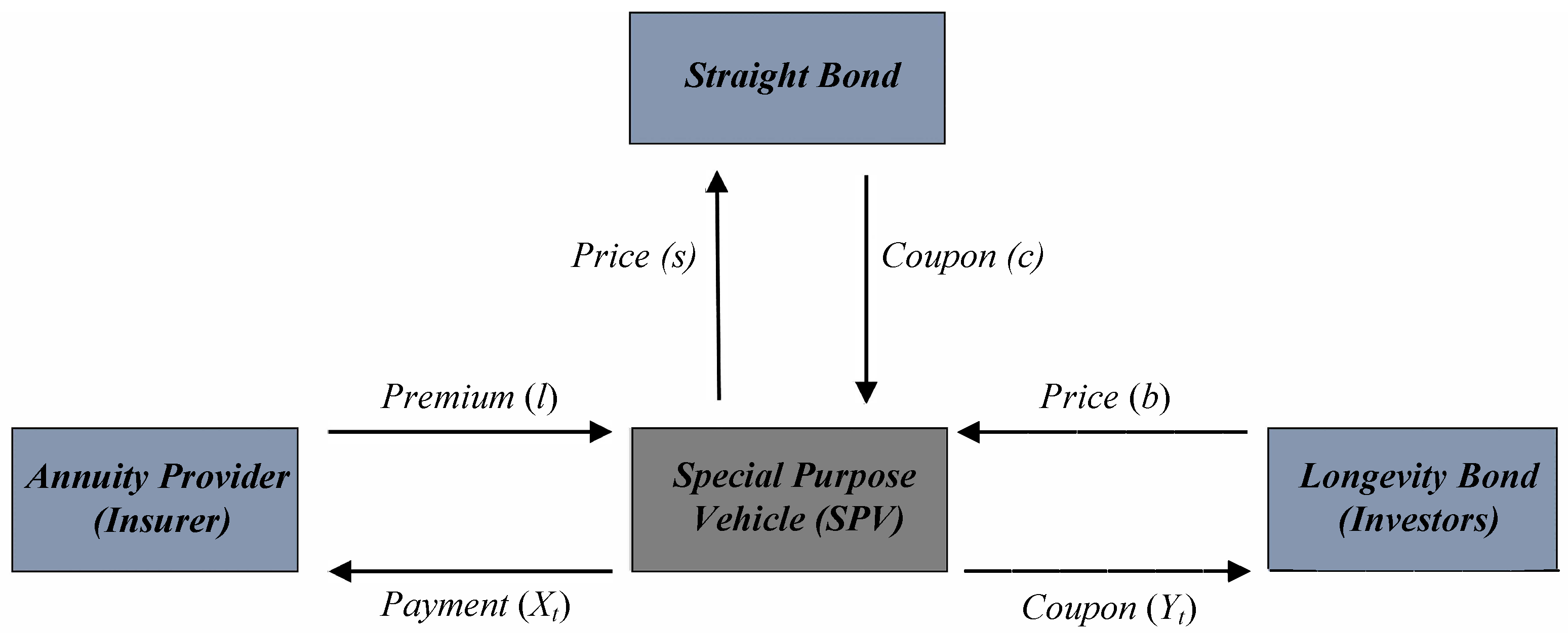
Consider that an annuity provider (insurer) pays a premium ${\displaystyle (p)}$ to purchase coverage from a special purpose vehicle (SPV), which issues a longevity bond at price ${\displaystyle (b)}$ to investors. Under this transaction, the risk is transferred from the annuity provider to the investors. The SPV invests the premium received from the annuity provider and the cash from the sale of the bonds to buy a default-free security, e.g., a straight bond at price ${\displaystyle (s)}$ with fixed annual coupons ${\displaystyle (c)}$ at each time ${\displaystyle t=1,2,\cdots ,T}$ and principal repayment ${\displaystyle (r)}$ at maturity ${\displaystyle T}$, such that ${\displaystyle s=r{(1+i)}^{-T}+\sum _{t=1}^{T}c{(1+i)}^{-t}}$, where ${\displaystyle i}$ is the risk-free rate. Then, the coupons that the SPV collects from the straight bond must be equal to the benefits received by the annuity provider (denoted by ${\displaystyle X_t}$) and the total coupons received by the investors (denoted by ${\displaystyle Y_t}$), according to the following equation:

$$X_t+Y_t=c.$$

(6)

Figure 1 displays the transactions that SPV makes to convey the longevity risk from the annuity provider to the investors.

This transaction is profitable for the SPV if ${\displaystyle p+b\ge s}$; however, to meet its obligations, it is sufficient to assume ${\displaystyle p+b=s}$. Now, consider that an annuity provider has to pay a cohort of ${\displaystyle l_x}$ annuitants, all aged ${\displaystyle x}$ initially. For simplicity, the annual payment is set at one currency unit per annuitant. Throughout this paper, we assume that the annuity provider uses the point mortality projections obtained under the credibility framework.

Let ${\displaystyle l_{x+t}}$ denote the random number of annuitants who survive to year ${\displaystyle t}$, given by ${\displaystyle l_{x+t}=l_x·{}_t{p}_x}$, and ${\displaystyle {\widehat{l}}_{x+t}^{cred}}$ denote the estimated number of survivors the same year, given by ${\displaystyle {\widehat{l}}_{x+t}^{cred}=l_x·{}_t{\widehat{p}}_x^{cred}}$, where ${\displaystyle {}_t{\widehat{p}}_x^{cred}}$ is the t-year survival probability obtained under the credibility framework in (4). In each year ${\displaystyle t}$, the annuity provider receives premiums from ${\displaystyle {\widehat{l}}_{x+t}^{cred}}$ survivors, while the annuities that it has to pay are equal to ${\displaystyle l_{x+t}}$. Thus, the longevity bond is used to hedge the risk induced by the deviations between the annuity provider’s payout ${\displaystyle l_{x+t}}$ and the received premiums ${\displaystyle {\widehat{l}}_{x+t}^{cred}}$.

The loss experienced by the annuity provider at each year ${\displaystyle t}$ is given by ${\displaystyle l_{x+t}-{\widehat{l}}_{x+t}^{cred}=l_x(p_{x,t}-p_{x,t}^{cred})}$, if ${\displaystyle {}_t{p}_x>{}_t{\widehat{p}}_x^{cred}}$. Thus, if payments in year ${\displaystyle t}$ exceed the received premiums, the annuity provider collects the excess from the SPV, up to a maximum amount. To proceed to the pricing process, we must first define the quantities involved in the required transactions. From the annuity provider’s perspective, its benefits collected from the SPV in year ${\displaystyle t=1,2,\cdots ,T}$ are given by

$$X_t=\left\{\begin{array}{cc}c,\hfill & l_{x+t}>{\widehat{l}}_{x+t}^{cred}+c,\hfill \\ l_{x+t}-{\widehat{l}}_{x+t}^{cred},\hfill & {\widehat{l}}_{x+t}^{cred}<l_{x+t}\le {\widehat{l}}_{x+t}^{cred}+c,\hfill \\ 0,\hfill & l_{x+t}\le {\widehat{l}}_{x+t}^{cred},\hfill \end{array}\right.$$

(7)

so that its net cash flows in year ${\displaystyle t}$ are

$$l_{x+t}-X_t=\left\{\begin{array}{cc}{l}_{x+t}-c,\hfill & l_{x+t}>{\widehat{l}}_{x+t}^{cred}+c,\hfill \\ {\widehat{l}}_{x+t}^{cred},\hfill & {\widehat{l}}_{x+t}^{cred}<l_{x+t}\le {\widehat{l}}_{x+t}^{cred}+c,\hfill \\ l_{x+t},\hfill & l_{x+t}\le {\widehat{l}}_{x+t}^{cred}.\hfill \end{array}\right.$$

From the perspective of the SPV, the longevity bond coupons ${\displaystyle Y_t=c-X_t}$ that are paid to investors in year ${\displaystyle t=1,2,\cdots ,T}$ are given by

$$Y_t=\left\{\begin{array}{cc}0,\hfill & l_{x+t}>{\widehat{l}}_{x+t}^{cred}+c,\hfill \\ c+{\widehat{l}}_{x+t}^{cred}-l_{x+t},\hfill & {\widehat{l}}_{x+t}^{cred}<l_{x+t}\le {\widehat{l}}_{x+t}^{cred}+c,\hfill \\ c,\hfill & l_{x+t}\le {\widehat{l}}_{x+t}^{cred}\hfill \end{array}\right.$$

(8)

3.2. Pricing with the Wang Transform under the Credibility Framework

The longevity risk market is usually referred to as incomplete, since its assets are not continuously traded, such as financial assets. As a result, a fair value of risk cannot be directly observed and other techniques should be utilized for pricing purposes. Wang (2000) introduced the Wang transform for pricing financial and insurance risks. This transform possesses various desirable properties and has a sound economic interpretation. For example, under specific assumptions, it recovers the capital asset pricing model and the Black–Scholes formula, while it is also consistent with Bühlmann’s premium principle. Chen et al. (2010) concluded that, among others, the Wang transform is preferable in pricing longevity risk, especially for long maturities. The Wang transform is defined by the following distortion operator

$$g_{\lambda }(F(t))=\mathsf{\Phi }\left[{\mathsf{\Phi }}^{-1}\left[F(t)\right]-\lambda \right],$$

where ${\displaystyle F(t)}$ is a given cumulative distribution function (cdf), ${\displaystyle \mathsf{\Phi }(x)}$ is the standard normal cdf, and ${\displaystyle \lambda }$ is a parameter called the market price of risk. We consider our projected life table under the credibility framework ${\displaystyle {}_t{\widehat{q}}_x^{cred}}$ in (5) as the physical distribution ${\displaystyle F(t)}$, which requires a distortion to obtain its transformed counterpart, denoted by ${\displaystyle {}_t{\tilde{q}}_x^{cred}}$, as follows

$${}_t{\tilde{q}}_x^{cred}=g_{\lambda }(F(t))=\mathsf{\Phi }\left[{\mathsf{\Phi }}^{-1}{(}_t{\widehat{q}}_x^{cred})-\lambda \right],$$

(9)

while the corresponding survival probability is given by

$${}_t{\tilde{p}}_x^{cred}=1-\mathsf{\Phi }\left[{\mathsf{\Phi }}^{-1}{(}_t{\widehat{q}}_x^{cred})-\lambda \right].$$

(10)

The value of market price of risk ${\displaystyle \lambda }$ is calculated by solving the following equation numerically

$$a_x^{market}=\sum _{t\ge 1}{(1+i)}^{-t}{}_t{\tilde{p}}_x^{cred}=\sum _{t\ge 1}{(1+i)}^{-t}\left[1-\mathsf{\Phi }[{\mathsf{\Phi }}^{-1}{(}_t{\widehat{q}}_x^{cred})-\lambda ]\right],$$

(11)

where ${\displaystyle a_x^{market}}$ is the observed annuity price for an annuitant aged ${\displaystyle x}$, and ${\displaystyle i}$ is the discount rate. Equation (11) indicates that the annuity market price accounts for the uncertainty in an annuitant’s future lifetime, given that mortality and interest rate risks are independent. Then, we can obtain the premium ${\displaystyle (p)}$ as the discounted expected value of the received benefits ${\displaystyle X_t}$ under the transformed probability measure as follows

$$p=\sum _{t=1}^T\tilde{E}(X_t){(1+i)}^{-t}$$

and by using (6), we can obtain the longevity bond price ${\displaystyle (b)}$ from

$$\begin{array}{ccc}\hfill b& =& s-p\hfill \\ & =& r{(1+i)}^{-T}+\sum _{t=1}^T\left[c-\tilde{E}(X_t)\right]{(1+i)}^{-t}\hfill \\ & =& r{(1+i)}^{-T}+\sum _{t=1}^T\tilde{E}(Y_t){(1+i)}^{-t},\hfill \end{array}$$

where ${\displaystyle \tilde{E}(X_t)}$ and ${\displaystyle \tilde{E}(Y_t)}$ denote the corresponding expected values of ${\displaystyle X_t}$ and ${\displaystyle Y_t}$, respectively, under the transformed distribution function. Thus, the calculation of these expected values is related to the distribution of ${\displaystyle l_{x+t}}$, which is the random number of an initial cohort of ${\displaystyle l_x}$ annuitants who survive to age ${\displaystyle x+t}$, with the transformed probability ${\displaystyle {}_t{\tilde{p}}_x^{cred}}$. This implies that ${\displaystyle l_{x+t}}$ follows a binomial distribution, with mean value ${\displaystyle l_x·{}_t{\tilde{p}}_x^{cred}}$ and variance ${\displaystyle l_x·{}_t{\tilde{p}}_x^{cred}·{}_t{\tilde{q}}_x^{cred}}$. However, the projected number of survivors ${\displaystyle {\widehat{l}}_{x+t}^{cred}}$ is not necessarily an integer value, so we need an approximation technique to calculate the transformed expected values. For example, since ${\displaystyle l_x}$ is large enough, ${\displaystyle l_{x+t}}$ can be approximately distributed as normal2 with parameters ${\displaystyle \mu =l_x·{}_t{\tilde{p}}_x^{cred}}$ and ${\displaystyle {\sigma }^2=l_x·{}_t{\tilde{p}}_x^{cred}·{}_t{\tilde{q}}_x^{cred}}$.

4. Numerical Illustration

In this section, we illustrate longevity bond pricing using the projected life tables, constructed under the credibility framework. We use the data of the general population of Greece, obtained by the Human Mortality Database (2022), where the official Greek data are publicly available for a relatively short period of mortality observations (1981–2019), compared to the datasets of other developed countries. Similar data limitations are often the case when dealing with insurance datasets. The credibility modeling framework aims to capture underlying data trends, particularly when there is limited mortality experience from a specific age, and extensive experience from the entire age range. Credibility regression methods can, of course, be used on larger datasets as well.

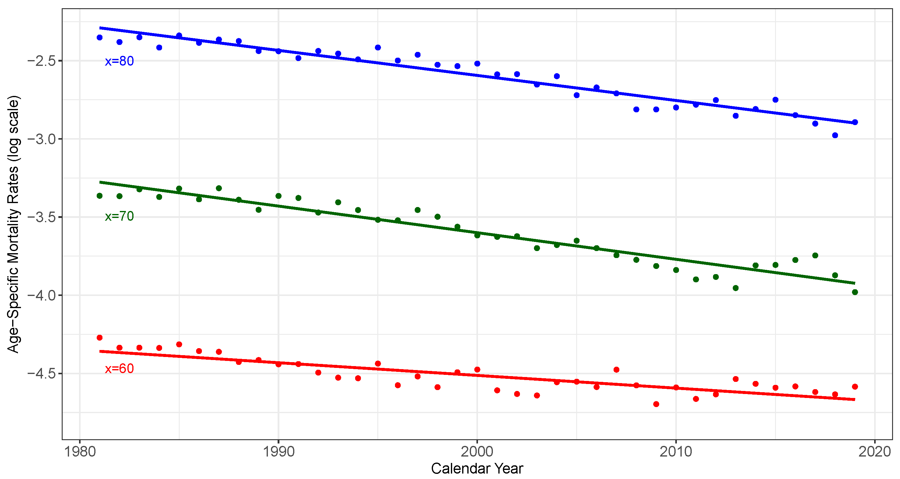
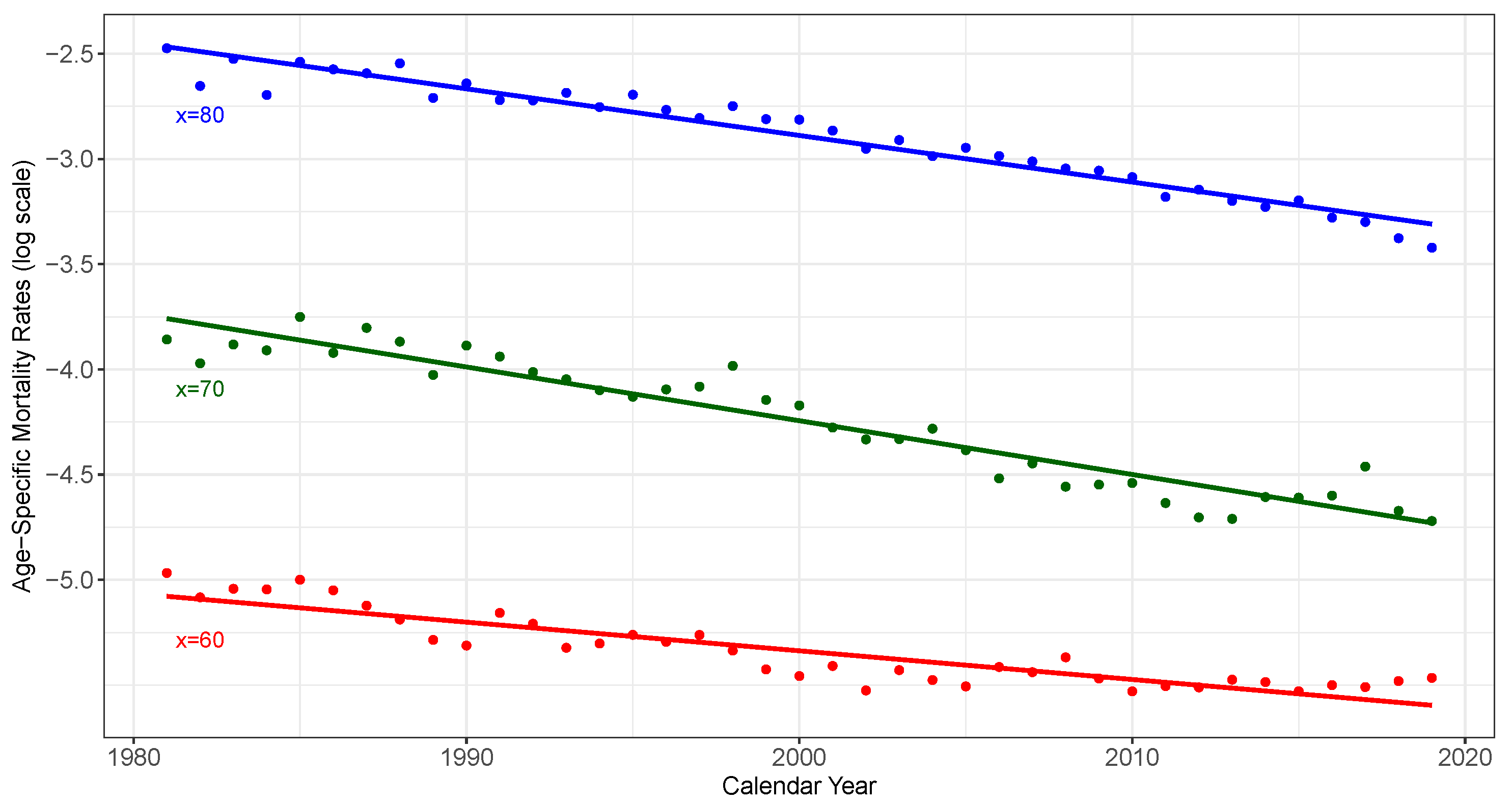
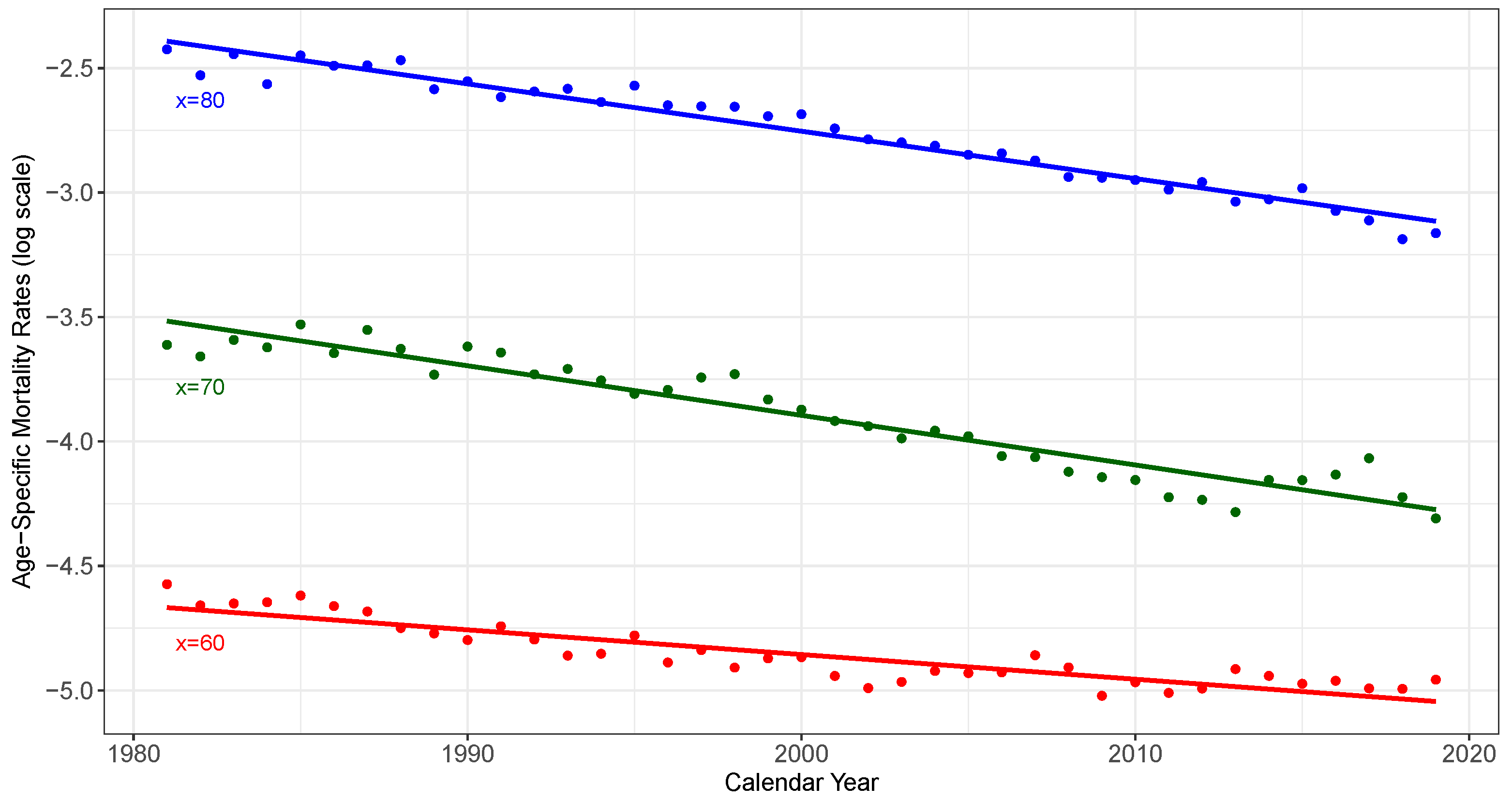
The Greek mortality rates for ages ${\displaystyle 60,70,80}$ over the period 1981–2019 are depicted for males in Figure 2, for females in Figure 3, and for the total population in Figure 4. For both genders and the total population, we can easily observe a downward trend in age-specific mortality data per year.

For our illustration, we construct projected life tables under the credibility regression framework, using the observed mortality rates in Greece, for males, females, and the total population for years ${\displaystyle [t_1,t_n]=[1981,2019]}$ and ages ${\displaystyle [x_1,x_k]=[55,84]}$ (from a usual age of an annuitant up to the level of life expectancy in developed countries). The forecasting performance of each projection method, in comparison to other widely used mortality models, has been thoroughly evaluated in Bozikas and Pitselis (2019), where the MPM method had the best average forecasting performance, especially in pricing annuity and life insurance products.

Let us now consider an initial cohort of ${\displaystyle l_x}$ = 10,000 annuitants in year ${\displaystyle 2020}$ of an annuity provider that needs to be secured for ${\displaystyle 20}$ years on. The ${\displaystyle a_{65}^{market}}$ value in Equation (11) is an appropriate proxy for the market price of an annuity, sold to an annuitant at the age of ${\displaystyle x=65}$. To obtain this value3, we use two representative life tables, developed by the Hellenic Actuarial Society (namely HAS2005 and HAS2012) for annuity products. The first life table is a sex-distinct table based on the mortality experience over the years 2000–2003 from individual insurance policies, while the second one, which is currently in use, is an updated version of HAS2005 developed on a unisex basis4. To ensure the efficiency of these life tables in future computations, the assigned working group projected the annual mortality improvement coefficients based on the data from the Greek general population.

To obtain the corresponding market price of risk ${\displaystyle \lambda }$ under each projection method, we use the projected probability ${\displaystyle {}_t{\widehat{q}}_{65}^{cred}}$ in (5) to solve Equation (11) numerically. The annuity values, based on the HAS2005 life table, are 14.66 for a male and 17.36 for a female annuitant aged 65, while the corresponding value for the total population, based on the HAS2012 table, is 16.54. The discount factor is calculated with ${\displaystyle i=2\%}$ for a period of ${\displaystyle T=20}$ years to maturity.

For comparison purposes, we consider different interest rates varying from 1 to 3 percent to calculate the market price of risk values under each projection method, based on the annuities obtained from the HAS2005 (male and female population) and HAS2012 life tables (total population). The corresponding results are exhibited in

Table 1. Market price of risk values under each projection method with ${\displaystyle i}$ varying from 1 to 3 percent.

Market Price of Risk${\displaystyle (\mathit{\lambda })}$
Projection method: SPM
Gender	Males	Females	Total
i = 1%	0.26172	0.36171	0.31084
i = 2%	0.22323	0.30706	0.27653
i = 3%	0.18933	0.25933	0.24518
Projection method: MPM
i = 1%	0.24500	0.33869	0.29373
i = 2%	0.20723	0.28599	0.25964
i = 3%	0.17404	0.23881	0.22922
Projection method: EPM
i = 1%	0.26160	0.36168	0.31075
i = 2%	0.22310	0.30702	0.27644
i = 3%	0.18919	0.25927	0.24508

.

We observe that the average market price of risk with the selected interest rate ${\displaystyle i=2\%}$ is ${\displaystyle 0.22}$ for males, ${\displaystyle 0.30}$ for females, and ${\displaystyle 0.27}$ for the total population, with the highest values per gender observed under the SPM projection method. Moreover, the overall average for males and females is ${\displaystyle 0.26}$, slightly higher than the average value ${\displaystyle 0.23}$, reported for other markets in the literature (see Kim and Choi 2011; Lorson and Wagner 2014). As Denuit et al. (2007) pointed out, the market price of risk is lower if a more conservative life table is used by the annuity provider.

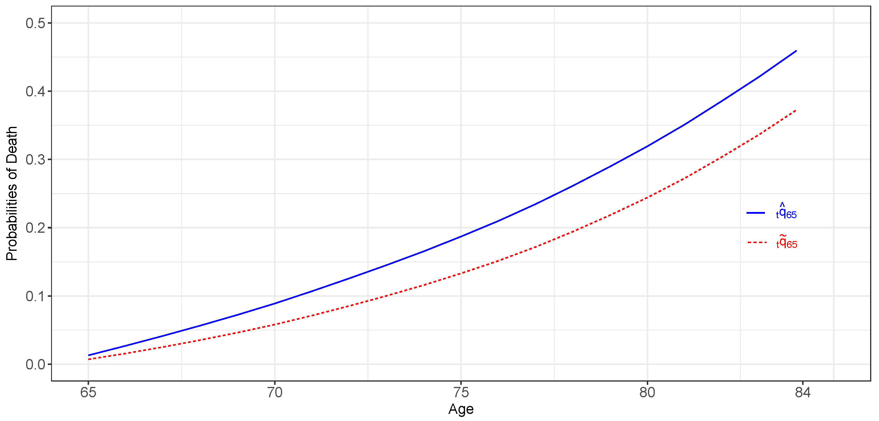
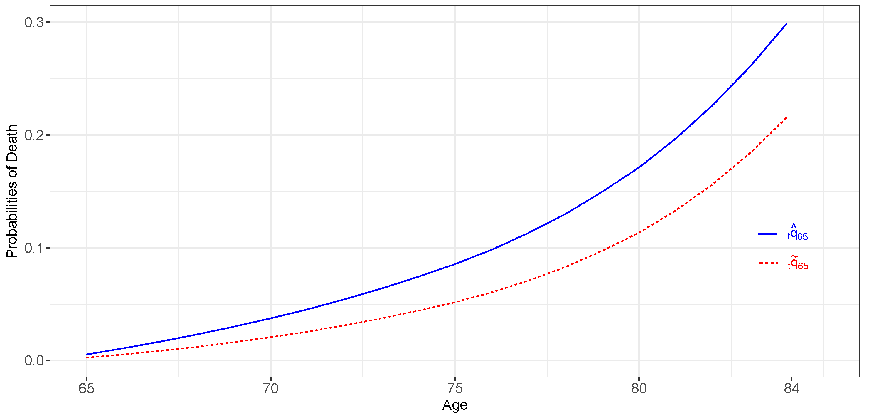
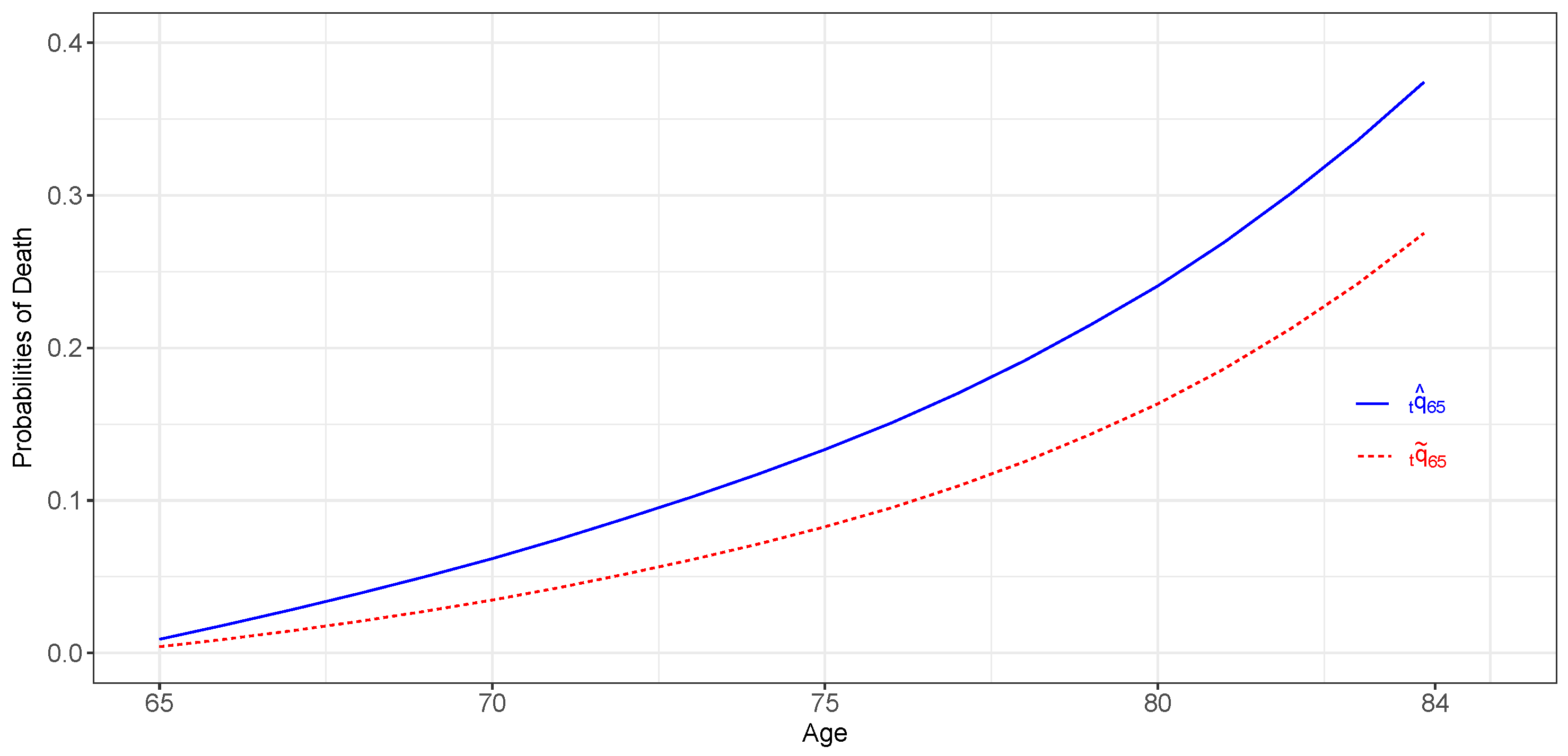
Once the ${\displaystyle \lambda }$s are obtained, we can obtain the transformed probability values by (9) and (10) to calculate the expected value ${\displaystyle \tilde{E}(Y_t)}$, needed for the calculation of the longevity bond price. The death probability ${\displaystyle {}_t{\widehat{q}}_{65}^{cred}}$ under the SPM method, which corresponds to a 65-year-old annuitant that will die before reaching age ${\displaystyle x+t=84}$, and the corresponding transformed probability ${\displaystyle {}_t{\tilde{q}}_{65}^{cred}}$ under the Wang transform are illustrated for Greek males in Figure 5, for females in Figure 6, and the total population in Figure 7.

We observe that the transformed probabilities are lower than their credibility counterparts. The same behavior is also observed for the corresponding probabilities under the MPM and EPM methods (not displayed). This was also noted by Levantesi et al. (2010), explaining the fact that transformed probabilities should be lower because they incorporate longevity risk.

Based on our initial cohort of ${\displaystyle l_x}$ = 10,000 annuitants, now, we assume that the SPV issues a longevity bond of face value 10,000,000 currency units with 4% coupon rate (${\displaystyle c=400}$) and at the same time buys a straight bond of the same price and coupon. The SPV’s annual payment is 1000 currency units per annuitant who survives. If the number of annuitants who survive ${\displaystyle l_{x+t}}$ exceeds the estimated number of survivors ${\displaystyle {\widehat{l}}_{x+t}^{cred}}$, the annuity provider collects the excess from the SPV, up to the maximum amount of 1000c = 400,000, while the the total coupon received by the investors is given by the ${\displaystyle max}$ (4,000,000 ${\displaystyle -X_t,0)}$. The longevity bond pricing results for males, females, and the total population are presented concisely in

Table 2. Longevity bond pricing results under each projection method based on males, females, and annuitants from the total population of Greece.

Pricing Results
Initial cohort of annuitants (${\displaystyle l_{65}}$)	10,000
Annual payment per annuitant	1000
Projection method: SPM
Gender	Males	Females	Total
Longevity bond price (b)	9,374,112	9,655,962	9,196,947
Premium value (p)	625,888	344,038	803,053
Projection method: MPM
Longevity bond price (b)	9,360,957	9,667,377	9,356,844
Premium value (p)	639,043	332,623	643,156
Projection method: EPM
Longevity bond price (b)	9,374,314	9,656,575	9,197,894
Premium value (p)	625,686	343,425	802,106

.

The pricing results indicate that the highest longevity bond price for a 65-year-old male annuitant from the initial cohort is given by the EPM method, while that for a female annuitant and an annuitant from the total population is given by the MPM method. This means that the premium paid by the annuity provider for a 20-year coverage for a male annuitant is lower under the EPM method (62.57), while the premium for a female and an annuitant from the total population is lower under the MPM method (33.26 and 64.32, respectively).

For the sake of comparison,

Table 3. The market price of risk and the longevity bond pricing results under the Lee–Carter method, based on males, females, and annuitants from the total population of Greece.

Pricing Results under the Lee–Carter Method
Gender	Males	Females	Total
Market price of risk (i = 2%)	0.2507	0.3493	0.3056
Longevity bond price (b)	9,008,307	9,305,596	8,942,833
Premium value (p)	991,693	694,404	1,057,167

provides the corresponding pricing results obtained by the well-known Lee and Carter (1992) mortality projection method. This method has been widely used in similar works for other markets—for example, see Denuit et al. (2007), Kim and Choi (2011) and Lorson and Wagner (2014). The results in Table 3 indicate that, for both genders and the total population of Greece, the Lee–Carter method leads to a higher market price of risk and premium values than those obtained by the proposed methods (Table 2).

In our application, the longevity bond price and the premium calculation are based on the mortality projections of the general population. This means that ${\displaystyle l_{x+t}}$ and ${\displaystyle {\widehat{l}}_{x+t}^{cred}}$ do not refer to a specific insured population, but derive from an official public database. From an investor’s perspective, the use of a public source gives full access to the data, avoiding moral hazard, since annuity providers cannot manipulate their reported mortality data. On the other hand, the use of general population mortality data may lead to an imperfect hedge, which introduces basis risk. It is worth noting that the premium value could be lower if our projection methods were applied only to mortality data of the insured population. However, this is practically impossible in our case as there are only three available life tables5 for the Greek insured population. Nevertheless, we think that a more active life annuity market could lead us to an even more representative price for the longevity bond.

5. Concluding Remarks

The increase in life expectancy raises serious concerns about the sustainability of the insurance industry. Longevity relates directly to the reserves of funds by creating additional costs for annuity providers.

In this paper, we exploited the credibility regression mortality framework to construct projected life tables with limited available data, and then we described how these projections can be incorporated to hedge longevity risk through the form of securitization. We demonstrated this process focusing on pricing a longevity bond using the available Greek data, obtained from a public source. To the best of our knowledge, such a study has not yet been conducted for Greek data; nevertheless, our findings look reasonable and conform with the international experience from similar studies.

Specifically, we used three methods under the credibility regression framework to construct projected life tables, and we described the process inherent to pricing a longevity bond. To obtain the transformed probabilities needed for the pricing process, we used the (one-parameter) Wang transform. Even if the Wang transform has been widely applied in the literature (see Lin and Cox 2005, Denuit et al. 2007, Levantesi et al. 2008, Kim and Choi 2011, and Lorson and Wagner 2014) to price longevity risk for different populations, some authors have raised their concerns in regard to the relationship between transforms of different cohorts and terms to maturity, and their mutual coherence (see Cairns et al. 2006). To resolve this issue, Wang (2002) proposed a two-parameter transform, using the cumulative distribution function of ${\displaystyle t}$ distribution instead of the standard normal distribution, but this transform seemed to lack a sound economic interpretation.

An alternative option in pricing and hedging financial derivatives is the use of the martingale approach. However, as Loisel and Serant (2007) noted, the life insurance market is far from complete due to a lack of observed market prices. Thus, the choice of an explicit risk-neutral measure is a non-trivial task, and this is the reason that traditional pricing methods, involving the Wang transform, are sometimes preferred to other classical financial methods. Nevertheless, the consideration of other approaches (e.g., two-parameter Wang transform, risk-neutral approach), under the credibility mortality framework, has been left for future research.

Regarding some extensions of the longevity risk securitization process in the public sector, it should be mentioned that in the near past, actuaries disagreed on whether longevity bonds should be issued by the government and others suggested that it should have an auxiliary role in sharing longevity risk. Nowadays, many actuaries agree that government-issued longevity bonds or other securities should be reconsidered as a tool of sharing longevity risk fairly between generations, leading to more secure pension savings for social welfare improvements.

References

- Barrieu, Pauline, Harry Bensusan, Nicole El Karoui, Caroline Hillairet, Stéphane Loisel, Claudia Ravanelli, and Yahia Salhi. 2012. Understanding, Modeling and Managing Longevity Risk: Key Issues and Main Challenges. Scandinavian Actuarial Journal 3: 203–31. [Google Scholar] [CrossRef] [Green Version]
- Blake, David, and Andrew J. G. Cairns. 2021. Longevity risk and capital markets: The 2019-20 update. Insurance: Mathematics and Economics 99: 395–439. [Google Scholar]
- Blake, David, and Williams Burrows. 2001. Survivor bonds: Helping to hedge mortality risk. The Journal of Risk and Insurance 68: 339–48. [Google Scholar] [CrossRef]
- Blake, David, Andrew J. G. Cairns, and Kevin Dowd. 2006. Living with mortality: Longevity bonds and other mortality-linked securities. British Actuarial Journal 12: 153–97. [Google Scholar] [CrossRef] [Green Version]
- Bozikas, Apostolos, and Georgios Pitselis. 2019. Credible regression approaches to forecast mortality for populations with limited data. Risks 7: 27. [Google Scholar] [CrossRef] [Green Version]
- Brouhns, Natacha, Michel Denuit, and Jeroen K. Vermunt. 2002. A Poisson log-bilinear regression approach to the construction of projected lifetables. Insurance: Mathematics and Economics 31: 373–93. [Google Scholar] [CrossRef] [Green Version]
- Cairns, Andrew J. G., David Blake, and Kevin Dowd. 2006. Pricing Death: Frameworks for the Valuation and Securitization of Mortality Risk. ASTIN Bulletin 36: 79–120. [Google Scholar] [CrossRef] [Green Version]
- Chen, Bingzheng, Lihong Zhang, and Lin Zhao. 2010. On the robustness of longevity risk pricing. Insurance: Mathematics and Economics 47: 358–73. [Google Scholar] [CrossRef]
- Cowley, Alex, and David Cummins. 2005. Securitization of life insurance assets and liabilities. The Journal of Risk and Insurance 72: 193–226. [Google Scholar] [CrossRef]
- De Jong, Piet, and Shauna Ferris. 2019. SM bonds—A new product for managing longevity risk. The Journal of Risk and Insurance 86: 121–49. [Google Scholar] [CrossRef]
- De Vylder, Etienne. 1978. Parameter estimation in credibility theory. ASTIN Bulletin 10: 99–112. [Google Scholar] [CrossRef] [Green Version]
- De Vylder, Etienne. 1996. Advanced Risk Theory: A Self-Contained Introduction. Paris: Editions de L’Université de Bruxelles. [Google Scholar]
- Denuit, Michel, Pierre Devolder, and Anne-Cécile Goderniaux. 2007. Securitization of Longevity Risk: Pricing Survivor Bonds with Wang Transform in the Lee-Carter Framework. The Journal of Risk and Insurance 74: 87–113. [Google Scholar] [CrossRef]
- Goovaerts, Marc J., Rob Kaas, Angela Van Heerwaarden, and Thierry Bauwelinckx. 1990. Effective Actuarial Methods. Amsterdam: North-Holland. [Google Scholar]
- Hachemeister, Charles. 1975. Credibility for Regression Models with Application to Trend (Reprint). In Credibility: Theory and Applications. Edited by P. Kahn. New York: Academic Press, Inc., pp. 307–48. [Google Scholar]
- Hari, Norbert, Anja De Waegenaere, Bertrand Melenberg, and Theo E. Nijman. 2008. Longevity risk in portfolios of pension annuities. Insurance: Mathematics and Economics 42: 505–19. [Google Scholar] [CrossRef]
- Human Mortality Database. 2022. University of California, Berkeley (USA), and Max Planck Institute for Demographic Research (Germany). Available online: www.mortality.org (accessed on 5 January 2022).
- Jones, Gavin. 2013. Longevity Risk & Reinsurance. Society of Actuaries Reinsurance News. July. Available online: https://www.soa.org/globalassets/assets/library/newsletters/reinsurance-section-news/2013/july/rsn-2013-issue76-jones.pdf (accessed on 25 April 2022).
- Kim, Changki, and Yangho Choi. 2011. Securitization of longevity risk using percentile tranching. The Journal of Risk and Insurance 78: 885–906. [Google Scholar] [CrossRef]
- Kisser, Michael, John Kiff, Erik S. Oppers, and Mauricio Soto. 2012. The Impact of Longevity Improvements on US Corporate Defined Benefit Pension Plans. International Monetary Fund No. 12/170. Washington: Social Science Research Network. [Google Scholar]
- Lee, Ronald, and Lawrence Carter. 1992. Modeling and Forecasting US Mortality. Journal of the American Statistical Association 87: 659–71. [Google Scholar]
- Levantesi, Sussana, Massimiliano Menzietti, and Tiziana Torri. 2008. Longevity bonds: An application to the Italian annuity market and pension schemes. Paper presented at 18th International AFIR Colloquium, Rome, Italy, October 1–3. [Google Scholar]
- Levantesi, Susanna, Massimiliano Menzietti, and Tiziana Torri. 2010. The securitization of longevity risk in pension schemes: The case of Italy. In Pension Fund Risk Management: Financial and Actuarial Modeling. Edited by Marco Micocci, Greg N. Gregoriou and Giovanni Batista Masala. CRC Finance Series; New York: Chapman-Hall, pp. 331–62. [Google Scholar]
- Lin, Tzuling, Cary Chi-Liang Tsai, and Hung-Wen Cheng. 2022. Asset Liability Management of Longevity and Interest Rate Risks: Using Survival–Mortality Bonds. North American Actuarial Journal. [Google Scholar] [CrossRef]
- Lin, Yijia, and Samuel H. Cox. 2005. Securitization of Mortality Risks in Life Annuities. The Journal of Risk and Insurance 72: 227–52. [Google Scholar] [CrossRef]
- Loisel, Stéphane, and Daniel Serant. 2007. In the Core of Longevity Risk: Dependence in Stochastic Mortality Models and Cut-Offs in Prices of Longevity Swaps. Working Paper. Villeurbanne: Université Lyon 1. [Google Scholar]
- Lorson, Jonas, and Joël Wagner. 2014. The pricing of hedging longevity risk with the help of annuity securitizations: An application to the German market. The Journal of Risk Finance 15: 385–416. [Google Scholar] [CrossRef] [Green Version]
- Renshaw, Arthur E., Steven Haberman, and Peter Hatzopoulos. 1996. The modelling of recent mortality trends in United Kingdom male assured lives. British Actuarial Journal 2: 449–77. [Google Scholar] [CrossRef]
- Thomsen, Jens, and Jens Verner Andersen. 2007. Longevity bonds—A financial market instrument to manage longevity risk. Denmark National Bank Monetary Review 4th Quarter 4: 29–44. [Google Scholar]
- Wang, Shaun. 2000. A Class of Distortion Operations for Pricing Financial and Insurance Risks. The Journal of Risk and Insurance 67: 15–36. [Google Scholar] [CrossRef] [Green Version]
- Wang, Shaun. 2002. A universal framework for pricing financial and insurance risks. Astin Bulletin 32: 213–34. [Google Scholar] [CrossRef] [Green Version]
- Yang, Sharon S., and Hong-Chih Huang. 2009. The Impact of Longevity Risk on the Optimal Contribution Rate and Asset Allocation for Defined Contribution Pension Plans. The Geneva Papers on Risk and Insurance—Issues and Practice 34: 660–81. [Google Scholar] [CrossRef] [Green Version]
Figure 1.
Transactions of the special purpose vehicle.
Figure 2.
Observed values of males in Greece, for ages 60, 70, 80, over the period 1981–2019. The straight lines denote the trend in mortality decline.
Figure 3.
Observed values of females in Greece, for ages 60, 70, 80, over the period 1981–2019. The straight lines denote the trend in mortality decline.
Figure 4.
Observed values of the total population in Greece, for ages 60, 70, 80, over the period 1981–2019. The straight lines denote the trend in mortality decline.
Figure 5.
Death probabilities and under the SPM method for males.
Figure 6.
Death probabilities and under the SPM method for females.
Figure 7.
Death probabilities and under the SPM method for the total population.