Linear Regression for Heavy Tails

1
Department of Mathematics, Universiteit van Amsterdam, 1098xh Amsterdam, The Netherlands
2
RiskLab, Department of Mathematics, ETH Zurich, 8092 Zurich, Switzerland
*
Author to whom correspondence should be addressed.
Risks 2018, 6(3), 93; https://0-doi-org.brum.beds.ac.uk/10.3390/risks6030093
Submission received: 29 June 2018
/
Revised: 18 August 2018
/
Accepted: 21 August 2018
/
Published: 10 September 2018
(This article belongs to the Special Issue Heavy Tailed Distributions in Economics)
Abstract
:There exist several estimators of the regression line in the simple linear regression: Least Squares, Least Absolute Deviation, Right Median, Theil–Sen, Weighted Balance, and Least Trimmed Squares. Their performance for heavy tails is compared below on the basis of a quadratic loss function. The case where the explanatory variable is the inverse of a standard uniform variable and where the error has a Cauchy distribution plays a central role, but heavier and lighter tails are also considered. Tables list the empirical sd and bias for ten batches of one hundred thousand simulations when the explanatory variable has a Pareto distribution and the error has a symmetric Student distribution or a one-sided Pareto distribution for various tail indices. The results in the tables may be used as benchmarks. The sample size is n = 100 but results for n = ∞ are also presented. The error in the estimate of the slope need not be asymptotically normal. For symmetric errors, the symmetric generalized beta prime densities often give a good fit.
| Contents | |
| 1 Introduction | 2 |
| 2 Background | 6 |
| 3 Three Simple Estimators: LS, LAD and RMP | 12 |
| 4 Weighted Balance Estimators | 21 |
| 4.1 Three Examples . . . . . . . . . . . . . . . . . . . . . . . . . . . . . . . . . . . . . . . . . . . . . . . . . . . . . . . . . . . . | 21 |
| 4.2 The Monotonicity Lemma . . . . . . . . . . . . . . . . . . . . . . . . . . . . . . . . . . . . . . . . . . . . . . . . . . . . . . . . | 22 |
| 4.3 LAD as a Weighted Balance Estimator . . . . . . . . . . . . . . . . . . . . . . . . . . . . . . . . . . . . . . . . . . . . . . . . . . | 25 |
| 4.4 Variations on LAD: LADPC, LADGC, and LADHC . . . . . . . . . . . . . . . . . . . . . . . . . . . . . . . . . . . . . . . . . . . . . . | 26 |
| 5 Theil’s Estimator and Kendall’s | 27 |
| 6 Trimming | 28 |
| 7 Tables | 31 |
| 7.1 The Empirical sd and Bias . . . . . . . . . . . . . . . . . . . . . . . . . . . . . . . . . . . . . . . . . . . . . . . . . . . . . . . | 32 |
| 7.2 Parameter Values . . . . . . . . . . . . . . . . . . . . . . . . . . . . . . . . . . . . . . . . . . . . . . . . . . . . . . . . . . . | 36 |
| 7.3 An Example . . . . . . . . . . . . . . . . . . . . . . . . . . . . . . . . . . . . . . . . . . . . . . . . . . . . . . . . . . . . . . | 38 |
| 8 Conclusions | 40 |
| A Tails | 43 |
| A.1 Tails of . . . . . . . . . . . . . . . . . . . . . . . . . . . . . . . . . . . . . . . . . . . . . . . . . . . . . . . . . . . | 43 |
| A.2 Tails of . . . . . . . . . . . . . . . . . . . . . . . . . . . . . . . . . . . . . . . . . . . . . . . . . . . . . . . . . . . | 44 |
| A.3 Tails of . . . . . . . . . . . . . . . . . . . . . . . . . . . . . . . . . . . . . . . . . . . . . . . . . . . . . . . . . . | 45 |
| A.4 Tails of . . . . . . . . . . . . . . . . . . . . . . . . . . . . . . . . . . . . . . . . . . . . . . . . . . . . . . . . . . | 46 |
| A.5 The Left Tail of . . . . . . . . . . . . . . . . . . . . . . . . . . . . . . . . . . . . . . . . . . . . . . . . . . . . . . . . . | 49 |
| B The Poisson Point Process Model | 50 |
| B.1 Distributions and Densities of Poisson Point Processes . . . . . . . . . . . . . . . . . . . . . . . . . . . . . . . . . . . . . . . . | 50 |
| B.2 Equivalence of the Distributions for ξ > 1/2. . . . . . . . . . . . . . . . . . . . . . . . . . . . . . . . . . . . . . . . . . | 52 |
| B.3 Error Densities with Local Irregularities . . . . . . . . . . . . . . . . . . . . . . . . . . . . . . . . . . . . . . . . . . . . . . | 53 |
| B.4 Two Plots . . . . . . . . . . . . . . . . . . . . . . . . . . . . . . . . . . . . . . . . . . . . . . . . . . . . . . . . . . . . . . | 54 |
| B.5 Convergence for the LS Estimates . . . . . . . . . . . . . . . . . . . . . . . . . . . . . . . . . . . . . . . . . . . . . . . . . . . | 57 |
| B.6 Convergence for the RM Estimates . . . . . . . . . . . . . . . . . . . . . . . . . . . . . . . . . . . . . . . . . . . . . . . . . . . | 59 |
| C The EGBP Distributions | 61 |
| C.1 The Exponential Generalized Beta Prime Densities . . . . . . . . . . . . . . . . . . . . . . . . . . . . . . . . . . . . . . . . . . . | 61 |
| C.2 Basic Formulas . . . . . . . . . . . . . . . . . . . . . . . . . . . . . . . . . . . . . . . . . . . . . . . . . . . . . . . . . . . . | 63 |
| C.3 The Closure of EGBP . . . . . . . . . . . . . . . . . . . . . . . . . . . . . . . . . . . . . . . . . . . . . . . . . . . . . . . . . | 64 |
| C.4 The Symmetric Generalized Beta Prime Distributions . . . . . . . . . . . . . . . . . . . . . . . . . . . . . . . . . . . . . . . . . . | 65 |
| C.5 The Parameters . . . . . . . . . . . . . . . . . . . . . . . . . . . . . . . . . . . | 66 |
| C.6 Fitting EGBP Distributions to Frequency Plots of log . . . . . . . . . . . . . . . . . . . . . . . . . . . . . . . . . . | 66 |
| C.7 Variations in the Error Density at the Origin . . . . . . . . . . . . . . . . . . . . . . . . . . . . . . . . . . . . . . . . . . . . | 69 |
| References | 71 |
1. Introduction
The paper treats the simple linear regression
when the errors are observations from a heavy tailed distribution, and the explanatory variables Xi too.
In linear regression, the explanatory variables are often assumed to be equidistant on an interval. If the values are random, they may be uniformly distributed over an interval or normal or have some other distribution. In this paper, the explanatory variables are random. The Xi are inverse powers of uniform variables Ui in (0,1): . The variables Xi have a Pareto distribution with tail index ξ > 0. The tails become heavier as the index increases. For ξ ≥ 1, the expectation is infinite. We assume that the error variables have heavy tails too, with tail index η > 0. The aim of this paper is twofold:
- The paper compares a number of estimators E for the regression line in the case of heavy tails. The distribution of the error is Student or Pareto. The errors are scaled to have InterQuartile Distance IQD = 1. The tail index ξ of the Pareto distribution of the explanatory variable varies between zero and three; the tail index η of the error varies between zero and four. The performance of an estimator E is measured by the loss function L(u) = u2 applied to the difference between the slope a of the regression line and its estimate . Our approach is unorthodox. For various values of the tail indices ξ and η, we compute the average loss for ten batches of a hundred thousand simulations of a sample of size one hundred. Theorems and proofs are replaced by tables and programs. If the error has a symmetric distribution, the square root of the average loss is the empirical sd (standard deviation). From the tables in Section 7, it may be seen that, for good estimators, this sd depends on the tail index of the explanatory variables rather than the tail index of the error. As a rule of thumb, the sd is of the order of1/10ξ + 1 0 ≤ ξ ≤ 3, 0 ≤ η ≤ 4, n = 100.This crude approximation is also valid for errors with a Pareto distribution. It may be used to determine whether an estimator of the regression line performs well for heavy tails.
- The paper introduces a new class of non-linear estimators. A weighted balance estimator of the regression line is a bisector of the sample. For even sample size half the points lie below the bisector, half above. There are many bisectors. A weight sequence is used to select a bisector which yields a good estimate of the regression line. Weighted balance estimators for linear regression may be likened to the median for univariate samples. The LAD (Least Absolute Deviation) estimator is a weighted balance estimator. However, there exist weighted balance estimators which perform better when the explanatory variable has heavy tails.
The results of our paper are exemplary rather than analytical. They describe the outcomes of an initial exploration on estimators for linear regression with heavy tails. The numerical results in the tables in Section 7 may be regarded as benchmarks. They may be used to measure the performance of alternative estimators. Insight in the performance of estimators of the regression line for samples of size one hundred where the explanatory variable has a Pareto distribution and the error a Student or Pareto distribution may help to select a good estimator in the case of heavy tails.
The literature on the LAD(Least Absolute Deviation) estimator is extensive (see Dielman (2005)). The theory for the TS (Theil–Sen) estimator is less well developed, even though TS is widely used for data which may have heavy tails, as is apparent from a search on the Internet. A comparison of the performance of these two estimators is overdue.
When the tail indices ξ and η are positive, outliers occur naturally. Their effect on estimates has been studied in many papers. A major concern is whether an outlier should be accepted as a sample point. In simulations, contamination does not play a role. In this paper, outliers do not receive special attention. Robust statistics does not apply here. If a good fairy were to delete all outliers, that would incommode us. It is precisely the outliers which allow us to position the underlying distribution in the (ξ,η)-domain and select the appropriate estimator. Equation (2) makes no sense in robust regression. Our procedure for comparing estimators by computing the average loss over several batches of a large number of simulations relies on uncontaminated samples. This does not mean that we ignore the literature on robust regression. Robust regression estimates may serve as initial estimates. (This approach does not do justice to the special nature of robust regression, which aims at providing good estimates of the regression line when working with contaminated data.) In our paper, we have chosen a small number of geometric estimators of the regression line, whose performance is then compared for a symmetric and an asymmetric error distribution at various points in the ξ,η-domain, see Figure 1a. In robust regression, one distinguishes M-, R- and L-estimators. We treat the M-estimators LS and LAD. These minimize the distance of the residuals for p = 2 and p = 1, respectively. We have not looked at other values of p ∈ [1,∞). Tukey’s biweight and Huber’s Method are non-geometric M-estimators since the estimate depends on the scaling on the vertical axis. The R-estimators of Jaeckel and Jurečková are variations on the LAD estimator. They are less sensitive to the behaviour of the density at the median, as we show in Section 3. They are related to the weighted balance estimators WB40, and are discussed in Section 4. Least Trimmed Squares (LTS) was introduced in Rousseeuw (1984). It is a robust version of least squares. It is a geometric L estimator. Least Median Squares introduced in the same paper yields the central line of a closed strip containing fifty of the hundred sample points. It selects the strip with minimal vertical width. If the error has a symmetric unimodal density one may add the extra condition that there are twenty five sample points on either side of the strip. This estimator was investigated in a recent paper Postnikov and Sokolov (2015). Maximum Likelihood may be used if the error distribution is known. We are interested in estimators which do not depend on the error distribution, even though one has to specify a distribution for the error in order to measure the performance. Nolan and Ojeda-Revah (2013) uses Maximum Likelihood to estimate the regression line when the errors have a stable distribution and the explanatory variable (design matrix) is deterministic. The paper contains many references to applications. The authors write: “In these applications, outliers are not mistakes, but an essential part of the error distribution. We are interested in both estimating the regression coefficients and in fitting the error distribution.” These words also give a good description of the aim of our paper.
There is one recent paper which deserves special mention. It uses the same framework as our paper. In Samorodnitsky et al. (2007), the authors determined limit distributions for the difference for certain linear estimators for the linear regression . The error Y* is assumed to have a symmetric distribution with power tails, and the absolute value of the explanatory variable also has a power tail. The tail indices are positive. The estimators are linear expressions in the error terms and functions of the absolute value of the explanatory variables (which in our paper are assumed to be positive):
The estimator E = Eθ depends on a parameter θ > 1 . The value θ = 2 yields LS. The paper distinguishes seven subregions in the positive (ξ,η)-quadrant with different rates of convergence. The paper is theoretical and focuses on the limit behaviour of the distribution of the estimator when the sample size tends to infinity. We look at the same range of values for the tail indices ξ and η, but our approach is empirical. We focus on estimators which perform well in terms of the quadratic loss function L(u) = u2. Such estimators are non-linear. We allow non-symmetric error distributions, and our regression line may have a non-zero abscissa. We only consider two classes of dfs for the error term, Student and Pareto, and our explanatory variables have a Pareto distribution. We restrict attention to the rectangle, (ξ,η) ∈ [0,3] × [0,4]. In our approach, the horizontal line η = 1/2 and the vertical line ξ = 1/2 turn out to be critical, but for ξ,η ≥ 1/2 the performance of the estimators depends continuously on the tail indices. There are no sharply defined subregions where some estimator is optimal. Our treatment of the behaviour for n → ∞ is cursory. The two papers present complementary descriptions of linear regression for heavy tails.
Let us give a brief overview of the contents. The exposition in Section 2 gives some background and supplies the technical details for understanding the results announced above. The next four sections describe the estimators which are investigated in our paper. The first describes the three well-known estimators LS, LAD and RMP. Least Squares performs well for 0 ≤ η < 1/2 when the error has finite variance. Least Absolute Deviation performs well when ξ is small. The estimator RMP (RightMost Point) selects the bisector which passes through the rightmost sample point. Its performance is poor, but its structure is simple. The next section treats the Weighted Balance estimators. The third treats Theil’s estimator which selects the line such that Kendall’s tau vanishes for the residuals, rather than the covariance as for Least Squares. It also introduces a weighted version of the Theil–Sen estimator. The last of these four sections introduces four estimators based on trimming: the Weighted Least Trimmed Squares estimator, WLTS, a weighted version of the estimator introduced by Rousseeuw and described above, and three estimators which select a bisector for which a certain state function is minimal when the 25 furthest points above the bisector are trimmed and the furthest 25 below. For these three estimators, trimming is related to the procedure RANSAC proposed in Fischler and Bolles (1981) for image analysis.
The heart of our paper is the set of tables in Section 7 where for ξ = 0, 1/2, 1, 3/2, 2, 3 we compare the performance of different estimators. The errors have a Student or Pareto distribution. The tail index of these distributions varies over 0, 1/3, 1/2, 2/3, 1, 3/2, 2, 3, 4. To make the results for different values of the tail index η comparable, the errors are standardized so that their df F* satisfies
F*(−1/2) = 1/4 F*(1/2) = 3/4.
This ensures that the InterQuartile Distance is IQD = 1. There are three sets of six tables corresponding to the six values of the tail index of the explanatory variable, ξ = 0, 1/2, 1, 3/2, 2, 3.
- The first set of tables lists the empirical sd for LS, LAD, Power Corrected LAD, the Theil–Sen estimator and three estimators based on trimming, all for errors with a Student distribution. The estimators do not depend on the tail index of the error.
- The second set of tables lists the empirical sd for the Hyperbolic Correction of LAD, the Right Median, RM, the Hyperbolic Balance estimators HB0 and HB40, Weighted Theil–Sen, and Weighted Least Trimmed Squares, WLTS, all for errors with a Student distribution. The estimators contain parameters which depend on the value of the tail indices, ξ and η. Thus, the Right Median, RM, depends on an odd positive integer which tells us how many of the rightmost points are used for the median. In WLTS, there are three parameters, the number of sample points which are trimmed, and two positive real valued parameters which determine a penalty for deleting sample points which lie far to the right.
- The third set of tables does the same as the second, but here the errors have a Pareto distribution. Both the empirical sd and bias of the estimates are listed.
The estimators yielding the tables are simple functions of the 2n real numbers which determine the sample. Apart from a choice of the parameters they do not depend on the form of the distribution of the error or the explanatory variable. The results show a continuous dependence of the empirical sd on the tail indices ξ and η both for Student and for Pareto errors. The sd and the value of the parameters are different in the third set of tables (Pareto errors) and the second (Student errors) but the similarity of the performance of the estimators for these two error distributions suggests that the empirical sds in these tables will apply to a wide range of error densities. The fourth table lists the optimal values of the parameters for various estimators. The example in Section 7.3 shows how the techniques of the paper should be applied to a sample of size n = 231 if neither the values of the tail indices ξ and η nor the distribution of the error are known.
The results in the three tables are for sample size n = 100. The explanatory variables are independent observations from a Pareto distribution on (1,∞), with tail index ξ > 0, arranged in decreasing order. One may replace these by the hundred largest points in a Poisson point process on (0,∞) with a Pareto mean measure with the same tail index. This is done in Appendix B. A scaling argument shows that the slope of the estimate of the regression line for the Poisson point process is larger by a factor approximately 100ξ compared to the iid sample. For the Poisson point process the rule of thumb in Equation (2) for the sd of the slope for good estimators has to be replaced by
10ξ−1 0 ≤ ξ ≤ 3, 0 ≤ η ≤ 4, n = 100.
The performance decreases with ξ since the fluctuations in the rightmost point around the central value x = 1 increase and the remaining 99 sample points Xi, i > 1, with central value 1/iξ, tend to lie closer to the vertical axis as ξ increases and hence give less information about the slope of the regression line.
What happens if one uses more points of the point process in the estimate? For ξ ≤ 1/2, the full sequence of the points of the Pareto point process together with the independent sequence of errors determines the true regression line almost surely. The full sequence always determines the distribution of the error variable, but for errors with a Student distribution and ξ > 1/2 it does not determine the slope of the regression line. For weighted balance estimators, the step from n = 100 to ∞ is a small one. If ξ is large, say ξ ≥ 3/4, the crude Equation (4) remains valid for sample size n > 100.
Conclusions are formulated in Section 8. The Appendix contains three sections: Appendix A treats tails and shows when tails of Weighted Balance estimators are comparable to those of the error Y*, and when they have finite second moment; Appendix B gives a brief exposition of the alternative Poisson point process model; and Appendix C introduces EGBP distributions. These often give a surprisingly good fit to the distribution of the logarithm of the absolute value of for symmetric errors.
2. Background
In this paper, both the explanatory variables Xi and the errors in the linear regression
have heavy tails. The vectors(X1, …, Xn) and are independent; the are iid; and the Xi are a sample from a Pareto distribution on (1,∞) arranged in decreasing order:
Xn < ⋯ < X2 < X1.
The Pareto explanatory variables may be generated from the order statistics U1 < ⋯ < Un of a sample of uniform variables on (0,1) by setting . The parameter ξ > 0 is called the tail index of the Pareto distribution. Larger tail indices indicate heavier tails. The variables have tail index η. They typically have a symmetric Student t distribution or a Pareto distribution. For the Student distribution, the tail index η is the inverse of the degrees of freedom. At the boundary, η = 0 and the Student distribution becomes Gaussian, the Pareto distribution exponential.
The problem addressed in this paper is simple: What are good estimators of the regression line for a given pair (ξ,η) of positive power indices?
For η < 1/2, the variable Y* has finite variance and LS (Least Squares) is a good estimator. For ξ < 1/2, the Pareto variable X = 1/Uξ has finite variance. In that case, the LAD (Least Absolute Deviation) often is a good estimator of the regression line. Asymptotically it has a (bivariate) normal distribution provided the density of Y* is positive and continuous at the median, see Van de Geer (1988). What happens for (ξ,η) ∈ [1/2,∞)2? In the tables in Section 7, we compare the performance of several estimators at selected parameter values (ξ,η) for sample size n = 100. See Figure 1a. First, we give an impression of the geometric structure of the samples which are considered in this paper, and describe how such samples may arise in practice.
For large ξ, the distribution of the points Xi along the positive horizontal axis becomes very skewed. For ξ = 3 and a sample of a hundred . 1 Exclude the rightmost point. The remaining 99 explanatory variables then all lie in an interval which occupies less than one percent of the range. The point (X1,Y1) is a pivot. It yields excellent estimates of the slope if the absolute error is small. The estimator RMP (RightMost Point) may be expected to yield good results. This estimator selects the bisector which passes through (X1,Y1).
Definition 1.
A bisector of the sample is a line which divides the sample into two equal parts. For an even sample of size 2m, one may choose the line to pass through two sample points: m − 1 sample points then lie above the line and the same number below.
The estimator RMP will perform well most of the time but if Y* has heavy tails RMP may be far off the mark occasionally, even when η < ξ. What is particularly frustrating are situations like Figure 1b where RMP so obviously is a poor estimate.
Figure 1a shows the part of (ξ,η)-space to which we restrict attention in the present paper. For practical purposes, the square 0 ≤ ξ, η ≤ 3/2 is of greatest interest. The results for other values of ξ and η may be regarded as the outcome of stress tests for the estimators.
Often, the variables are interpreted as iid errors. It then is the task of the statistician to recover the linear relation between the vertical and horizontal coordinate from the blurred data for Y. The errors are then usually assumed to have a symmetric distribution, normal or stable.
There is a different point of view. For a bivariate normal vector (X,Y), there exists a line, the regression line y = b + ax, such that conditional on X = x the residual Y* = Y − (ax + b) has a centred normal distribution independent of x. A good estimate of the regression line will help to obtain a good estimate of the distribution of (X,Y). This situation may also occur for heavy-tailed vectors.
Heffernan and Tawn (2004) studies the distribution of a vector conditional on the horizontal component being large. In this conditional extreme value model, the authors focus on the case where the conditional distribution of Y given X = x is asymptotically independent of x for x → ∞. The vector Z = (X,Y) conditioned to lie in a half plane Ht = {x > t} is a high risk scenario, denoted by ZHt. Properly normalized, the high risk scenarios ZHt may have a limit distribution for t → ∞. From univariate extreme value theory, we know that the horizontal coordinate of the limit vector has a Pareto or exponential distribution. In the Heffernan–Tawn model, the vertical coordinate of the limit vector is independent of the horizontal coordinate. Heffernan and Tawn in Heffernan and Tawn (2004) considered vectors with light tails. The results were extended to heavy tails by Heffernan and Resnick in Heffernan and Resnick (2007). See Balkema and Embrechts (2007) for a list of all limit distributions.
Given a sample of a few thousand observations from a heavy-tailed bivariate distribution, one will select a subsample of say the hundred points for which the horizontal coordinate is maximal. This yields a sequence x1 > ⋯ > x100. The choice of the horizontal axis determines the vertical coordinate in the points (x1,y1), …, (x100,y100). In the Heffernan–Tawn model, the vertical coordinate may be chosen to be asymptotically independent of x for x → ∞. To find this preferred vertical coordinate, one has to solve the linear regression Equation (1). The residuals, , allow one to estimate the distribution of the error and the tail index η.
The model , where X1 > ⋯ > Xn are the extreme sample points and the vertical coordinates are asymptotically iid and independent of the values Xi, yields a nice bivariate extension of univariate Extreme Value Theory. In our analysis of the Heffernan-Tawn model, it became clear that good estimates of the slope of the regression line for heavy tails are essential if one wants to apply the model. The interpretation of the data should not effect the statistical analysis. Our interest in the Heffernan–Tawn model accounts for the Pareto distribution of the explanatory variable and the assumption of heavy tails for the error term. It also accounts for our focus on estimates of the slope.
We restrict attention to geometric estimators of the regression line. Such estimators are called contravariant in Lehmann (1983). A transformation of the coordinates has no effect on the estimate of the regression line L. It is only the coordinates which are affected.
Definition 2.
The group of affine transformations of the plane which preserve orientation and map right vertical half planes into right vertical half planes consists of the transformations
(x′, y′) = (px + q, ax + b + cy) p > 0, c > 0.
An estimator of the regression line is geometric if the estimate is not affected by coordinate transformations in .
Simulations are used to compare the performance of different estimators. For geometric estimators, one may assume that the true regression line is the horizontal axis, that the Pareto distribution of the explanatory variables Xi is the standard Pareto distribution on (1,∞) with tail , and that the errors are scaled to have IQD = 1. Scaling by the InterQuartile Distance IQD allows us to compare the performance of an estimator for different error distributions.
The aim of this paper is to compare various estimators of the regression line for heavy tails. The heart of the paper is the set of tables in Section 7. To measure the performance of an estimator E we use the loss function L(a) = a2. We focus on the slope of the estimated regression line . For given tail indices (ξ,η), we choose X = 1/Uξ Pareto and errors Y* with a Student or Pareto distribution with tail index η, scaled to have IQD = 1. We then compute the average loss Lr of the slope for r simulations of a sample of size n = 100 from this distribution. where the sum is taken over the outcomes for r simulations. We choose r = 105. The square root is our measure of performance. It is known as RMSE (Root Mean Square Error). We do not use this term. It is ambiguous. The mean may indicate the average, but also the expected value. Moreover, in this paper, the error is the variable Y* rather than the difference . If the df F* of Y* is symmetric, the square root is the empirical sd of the sequence of r outcomes of . The quantity γ is random. If one starts with a different seed, one obtains a different value γ. Since r is large. one may hope that the fluctuations in γ for different batches of r simulations is small. The fluctuations depend on the distribution of γ, and this distribution is determined by the tail of the random variable . The average loss Lr is asymptotically normal if L has a finite second moment. For this, the estimate has to have a finite fourth moment. In Section 3, the distribution of γ is analyzed for ξ = η = i/10, i = 2, …, 7, for the estimator E = LS and Student errors. We show how the distribution of γ changes on passing the critical value η = 1/2.
The fluctuations in γ are perhaps even more important than the average value in determining the quality of an estimator. To quantify the fluctuations in γ we perform ten batches of 105 simulations. This yields ten values γi for the empirical sd. Compute the average μ and the sd . The two quantities μ and δ describe the performance of the estimator. Approximate δ by one of
…, 20, 10, 5, 2, 1, 0.5, 0.2, 0.1, 0.05, 0.02, 0.01, 0.005, 0.002, 0.001, 0.0005, 0.0002, 0.0001, 0.00005,…
Now, approximate the pair (μ,δ) by (m/10k, d/10k) with d ∈ {1, 2, 5} and m an integer. For the representation (m/10k, d/10k), it suffices to know the integers m,k and the digit d ∈ {1, 2, 5}. In our case, δ typically is small, 0 < δ < 1 for estimators with good performance. In that case, k is non-negative and one can reconstruct m and k from the decimal fraction m/10k provided one writes out all k digits after the decimal point, including the zeros. That allows one to reconstruct the pair (m/10k, d/10k) from m/10k[d]. This lean notation is also possible if one writes m/10k as me − k, as in 17e + 6, the standard way to express seventeen million in R. In this paper, we often write m/10k[d] except when this notation leads to confusion. Here are some examples: For (μ, δ) = (0.01297, 0.000282), (136.731 × 10⁻⁷, 1.437 × 10⁻⁷), (221.386, 3.768), (221.386, 37.68) and (334567.89, 734567.89) the recipe gives:
0.0130[2] 137e − 7[1] 221[5] 220[50] 0e + 6[1].
Actually, we still have to say how we reduce δ to d/10k. Take d = 1; if 10kδ lies in [0.7, 1.5], d = 2 for 1.5 ≤ 10kδ < 3 and d = 5 for 3 ≤ 10kδ < 7. Finally, define . In Equation (6), the reader sees at a glance the average of the outcomes γi of the ten batches, and the magnitude of the fluctuations.
Let us mention two striking results of the paper. The first concerns LAD (Least Absolute Deviation), a widely used estimator which is more robust than LS (Least Squares) since it minimizes the sum of the absolute deviations rather than their squares. This makes the estimator less sensitive to outliers of the error. The LAD estimate of the regression line is a bisector of the sample. For ξ > 1/2, the outliers of the explanatory variable affect the stability of the LAD estimate (see Rousseeuw (1991), p. 11). Table 1 lists some results from Section 7 for the empirical sd of the LAD-estimate.
The message from the table is clear. For errors with infinite second moment, η ≥ 1/2, use LAD, but not when ξ ≥ 1/2. Actually, the expected loss for is infinite for η ≥ 1/2 for all ξ. In this respect LAD is no better than LS. If the upper tail of the error varies regularly with negative exponent, the quotient
is a bounded function on . See Theorem 2.
The discrepancy between the empirical sd, based on simulations, and the theoretical value is disturbing. Should a risk manager feel free to use LAD in a situation where the explanatory variable is positive with a tail which decreases exponentially and the errors have a symmetric unimodal density? Conversely, should she base her decision on the mathematical result in the theorem? The answer is clear: One hundred batches of a quintillion simulations of a sample of size n = 100 with X standard exponential and Y* Cauchy may well give outcomes which are very different from 0.0917[5]. Such outcomes are of no practical interest. The empirical sds computed in this paper and listed in the tables in Section 7 may be used for risks of the order of one in ten thousand, but for risks of say one in ten million—risks related to catastrophic events—other techniques have to be developed.
A million simulations allow one to make frequency plots which give an accurate impression of the density when a density exists. Such plots give more information then the empirical sd; they suggest a shape for the underlying distribution. We plot the log frequencies in order to have a better view of the tails. Log frequencies of Gaussian distributions yield concave parabolas. Figure 2 shows loglog frequency plots for two estimators of the regression line for errors with a symmetric Student distribution for (ξ,η) = (3,4). A loglog frequency plot of plots the log of the frequency of . It yields a plot with asymptotes with non-zero slopes if the df of has power tails at zero and infinity.
First, consider the loglog frequency plot of on the left. The range of in Figure 2a is impressive. The smallest value of |a| is of the order of 10−24, the largest of the order of 1020. A difference of more than forty orders of magnitude. Accurate values occur when X1 is large and |Y*| is small. The LAD estimate of the regression line is a bisector of the sample. In extreme cases it will pass through the rightmost point and agree with the RMP estimate. The value will then be of the order of 1/X1. The minimum is determined by the minimal value of 108 simulations of a standard uniform variable. For ξ = 3, this gives the rough value 10−24 for the most accurate estimate. Large values of |a| are due to large values of |Y1|. Because of the tail index η = 4, the largest value of |Y1| will be of the order of 1024. Then, |Y1|/X1 is of the order of 1018. For the tail index pair (ξ,η) = (3,4), the limits of computational accuracy for R are breached.
The asymptotes in the loglog frequency plots for correspond to power tails for , at the origin and at infinity. The slope of the asymptote is the exponent of the tail. The plot on the right, Figure 2b, shows that it is possible to increase the absolute slope of the right tail and thus reduce the inaccurate estimates. The value 0e+16[1] for the sd of the LAD estimate of the slope is reduced to 0.00027[5] for RM(21). The Right Median estimate RM(21) with parameter 21 is a variation on the Rightmost Point estimate RMP. Colour the 21 rightmost sample points red and then choose the bisector of the sample which also is a bisector of the red points. This is a discrete version of the cake cutting problem: “Cut a cake into two equal halves, such that the icing is also divided fairly.” The RM estimate passes through a red and a black point. Below the line are 49 sample points, ten of which are red; above the line too. The tail index of is at most 2η/20 = 0.4 by Theorem A2. The estimate has finite sd even though the value 0.00027[5] shows that the fluctuations in the empirical sd for ten batches of a hundred thousand simulations are relatively large.
The smooth red curve in the right hand figure is the EGBP fit to the log frequency plot of , see Appendix C.
The tables in Section 7 compare the performance of various estimators. It is not the value of the empirical sds listed in these tables which are important, but rather the induced ordering of the estimators. For any pair (ξ,η) and any estimator E, the empirical sd and the value of the parameter will vary when the df F* of the error Y* is varied, but the relative order of the estimators is quite stable as one sees by comparing the results for Student and Pareto errors with the same tail indices.
The remaining part of this section treats the asymptotic behaviour of estimators when the sample size tends to ∞ via a Poisson point process approach. This part may be skipped on first reading.
Recall that our interest in the problem of linear regression for heavy tails was triggered by a model in extreme value theory. One is interested in the behaviour of a vector X when a certain linear functional is large. What happens to the distribution of the high risk scenario for the half space Ht = {ζ ≥ t} for t → ∞? We consider the bivariate situation and choose coordinates such that ζ is the first coordinate. In the Heffernan–Tawn model, one can choose the second coordinate such that the two coordinates of the high risk scenario are asymptotically independent. More precisely there exist normalizations of the high risk scenarios, affine transformations mapping the vertical half plane Ht onto H1 such that the normalized high risk scenarios converge in distribution. The limit scenario lives on H1 = {x ≥ 1}. The first component of the limit scenario has a Pareto (or exponential) distribution and is independent of the second component. The normalizations which yield the limit scenario, applied to the samples, yield a limiting point process on {x > 0} (by the Extension Theorem, Theorem 14.12, in Balkema and Embrechts (2007).) If the limit scenario has density r(x)f*(y) on H1 with r(x) = λ/xλ + 1 on (1, ∞), the limit point process is a Poisson point process N0 with intensity r(x)f*(y) where r(x) = λ/xλ + 1 on (0, ∞). It is natural to use this point process N0 to model the hundred points with the maximal x-values in a large sample from the vector X.
For high risk scenarios, estimators may be evaluated by looking at their performance on the hundred rightmost points of this Pareto point process. For geometric estimators the normalizations linking the sample to the limit point process do not affect the regression line since the normalizations belong to the group used in the definition of geometric estimator above. The point process N0 actually is a more realistic model than an iid sample.
For geometric estimators, there is a simple relation between the slope An of the regression line for the n rightmost points ,i = 1, …, n, of the point process N0 and the slope of the regression line for a sample of n independent observations :
The first n points of the standard Poisson point process divided by the next point, Zn, are the order statistics from the uniform distribution on (0,1) and independent of the Gamma(n + 1) variable Zn with density xne−x/n! on (0,∞).) A simple calculation shows that ζn = nξ + c(ξ) + o(1) for n → ∞.
The point process Na with points , , has intensity r(x)f*(y − ax). The step from n to n + 1 points in estimating the linear regression means that one reveals the n + 1 st point of the point process Na. This point lies close to the vertical axis if n is large and very close if ξ > 0 is large too. The new point will give more accurate information about the abscissa b of the regression line than the previous points since the influence of the slope decreases. For the same reason, it will give little information on the value of the slope a. The point process approach allows us to step from sample size n = 100 to ∞ and ask the crucial question: Can one distinguish Na and N0 for a ≠ 0?
Almost every realization of Na determines the probability distribution of the error but it need not determine the slope a of the regression line. Just as one cannot distinguish a sequence of standard normal variables Wn from the sequence of shifted variables Wn + 1/n with absolute certainty, one cannot distinguish the Poisson point process Na from N0 for ξ > 1/2 and errors with a Student distribution. The distributions of the two point processes Na and N0 are equivalent. See Appendix B for details.
The equivalence of the distributions of Na and N0 affects the asymptotic behaviour of the estimates An of the slope of the regression line for the Poisson point process. There exist no estimators for which An converges to the true slope. The limit, if it exists, is a random variable A∞, and the loss (A∞ − a)2 is almost surely positive. Because of the simple scaling relation in Equation (7) between the estimate of the slope for iid samples and for N, the limit relation An ⇒ A∞ implies .
For errors with finite second moment, the sd σn of the slope of the LS estimate An of the regression line y = ax + b based on the n rightmost points of the Poisson point process has a simple expression in terms of the positions of the explanatory variables x1 > ⋯ > xn, as does the sd of the slope of the LS estimate of the regression ray y = ax (with abscissa b = 0). We assume standard normal errors and let R calculate the value of σn = σn(ξ) and for various values of n and of ξ ∈ (0,3]. Since the explanatory variables are random, we use a million simulations to approximate these deterministic values. We also compute approximations to (see Appendix B.5). The plots in Figure 3 will answer questions such as the following:
- How does σ∞ depend on ξ ∈ (0,3]?
- How much does the sd σn decrease if we reveal the next n points of the point process N0?
- What is the effect of the unknown abscissa on the estimates? For what n will σn equal ?
Figure A2 in Appendix B.4 shows the plots on a logarithmic scale and similar plots for the empirical sd of the Right Median estimates for Cauchy errors.
3. Three Simple Estimators: LS, LAD and RMP
Least Squares (LS) and Least Absolute Deviation (LAD) are classic estimators which perform well if the tail index η of the error is small (LS), or when the tail index ξ of the explanatory variable is small (LAD). For ξ,η ≥ 1/2, one may use the bisector of the sample passing through the RightMost Point (RMP) as a simple but crude estimate of the regression line.
At the critical value η = 1/2, the second moment of the error becomes infinite and the least squares estimator breaks down. Samples change gradually when ξ and η cross the critical value of 1/2. We investigate the break down of the LS estimator by looking at its behaviour for ξ = η = i/10, i = 2, …, 7, for errors with a Student distribution. It is shown that the notation in Equation (6) nicely expresses the decrease in the performance of the estimator on passing the critical exponent. We also show that even for bounded errors there may exist estimators which perform better than Least Squares. The estimator LAD is more robust than Least Squares. Its performance declines for ξ > 1/2, but even for ξ = 0 (exponential distribution) or ξ = −1 (uniform distribution) its good performance is not lasting. The RightMost Point estimate is quite accurate most of the time but may be far off occasionally. That raises the question whether an estimator which is far off 1% of the time is acceptable.
Least squares (LS) is simple to implement and gives good results for η < 1/2. Given the two data vectors x and y, we look for the point ax + be in the two-dimensional linear subspace spanned by x and e = (1, …, 1) which gives the best approximation to y. Set z = x − me where m is the mean value of the coordinates of x. The vectors e and z are orthogonal. Choose a0 and b0 such that y − a0z ⊥ z and y − b0e ⊥ e. Explicitly:
a0 = 〈y, z〉/〈z, z〉 b0 = 〈y, e〉/〈e, e〉.
The point we are looking for is
a0z + b0e = a0x + (b0 − ma0)e = ax + be.
This point minimizes the sum of the squared residuals, where the residuals are the components of the vector y − (ax + be). Note that m is the mean of the components of x and s2 = 〈z, z〉 the sample variance. Conditional on X = x, the estimate of the slope is
There is a simple relation between the standard deviation of Y* and of the estimate of the slope: (ζi) is a unit vector; hence conditional on the configuration x of X
If the sd of Y* is infinite then so is the sd of the estimator . That by itself does not disqualify the LS estimator. What matters is that the expected loss is infinite.
Let us see what happens to the average loss Lr when the number r of simulations is large for distributions with tail index ξ = η = τ as τ crosses the critical value 0.5 where the second moment of Y* becomes infinite. Figure 4 shows the log frequency plots of for ξ = η = τ(i) = i/10 for i = 2, …, 7 based on ten batches of a hundred thousand simulations. The variable Y* has a Student t distribution with 1/η degrees of freedom and is scaled to have interquartile distance one. The most striking feature is the change in shape. The parabolic form associated with the normal density goes over into a vertex at zero for τ = 0.5 suggesting a Laplace density, and a cusp for τ > 0.5. The cusp will turn into a singularity f(x) ∼ c/xτ with τ = 1 − 1/η > 0 when Y* has a Student distribution with tail index η > 1.
The change that really matters is not visible in Figure 4. It occurs in the tails.
The distribution of the average loss Lr depends on the tail behaviour of . The Student variable Y* with 1/η degrees of freedom has tails . This also holds for which is a mixture of linear combinations of these variables by Equation (9). For η = i/10, i = 2, …, 7, the positive variable has upper tail . See Theorem 1.
First, consider the behaviour of the average Zr(i) of r = 106 independent copies of the variable Z(i) = 1/Ui/5 where U is standard uniform. The Pareto variable Z(i) has tail 1/z5/i on (1, ∞). Its expectation is 2/3, 3/2, 4, ∞, ∞, ∞ for i = 2, 3, 4, 5, 6, 7. The average Zr(i) has the form mr(i) + sr(i)Wr(i) where one may choose mr(i) to be the mean of Z(i) if finite, and where Wr(i) converges in distribution to a centred normal variable for i = 2, and for i > 2 to a skew stable variable with index α = i/5 and β = 1. The asymptotic expression for Zr is:
Zr(i) = mr(i) + sr(i)Wr(i) i = 2, 3, 4, 5, 6, 7
i = 2: , , Wr(2) ⇒ c2W2;
i = 3: , sr(3) = r−2/5, Wr(3) ⇒ c3W5/3;
i = 4: , sr(4) = r−1/5, Wr(4) ⇒ c4W5/4;
i = 5: mr(5) = logr, sr(5) ≡ 1, Wr(5) ⇒ c5W1;
i = 6: mr(6) = sr(6) = r1/5, Wr(6) ⇒ c6W5/6; and
i = 7: mr(7) = sr(7) = r2/5, Wr(7) ⇒ c7W5/7.
For an appropriate constant Ci > 0, the variable has tails asymptotic to 1/t5/i, and hence the averages CiLr exhibit the asymptotic behaviour above. It is the relative size of the deterministic part mr(i) of Lr compared to the size of the fluctuations sr(i)Wr(i) of the random part which changes as i/10 passes the critical value 0.5. The quotients sr(i)/mr(i) do not change much if one replaces Lr by Lr, the batch sd. The theoretical results listed above are nicely reflected in the Hill estimate of the tail index, and the loss of precision in the empirical sds in Table 2.
For individual samples, it may be difficult to decide whether the parameters are ξ = η = 4/10 or 6/10. The pairs (4,4)/10 and (6,6)/10 belong to different domains in the classification in Samorodnitsky et al. (2007) but that classification is based on the behaviour for n → ∞. The relation between the estimates for (4,4)/10 and (6,6)/10 for samples of size n = 100 becomes apparent on looking at large ensembles of samples for parameter values (i,i)/10 when i varies from two to seven. The slide show was created in an attempt to understand how the change in the parameters affects the behaviour of the LS estimator. The estimate has a distribution which depends on the parameter. The dependence is clearly expressed in the tails of the distribution. The Hill estimates reflect nicely the tail index η of the error. A recent paper Mikosch and Vries (2013) gives similar results for samples with fixed size for LS in linear regression where the coefficient b in Equation (1) is random with heavy tails.
The simplicity of the LS estimator makes a detailed analysis of the behaviour of the average loss Lr possible for . The critical value is η = 1/2. The relative size of the fluctuations rather than the absolute size of the sd signal the transition across the critical value. Note that the critical value η = 1/2 is not due to the “square” in Least Squares but to the exponent 2 in the loss function. There is a simple relation between the tails of the error distribution and of . Appendix A.5 shows that is bounded. Lemma 3.4 in Mikosch and Vries (2013) then gives a very precise description of the tail behaviour of in terms of the tails of Y*. We formulate this lemma as a Theorem below.
Theorem 1. (Mikosch and de Vries)
Let denote the slope of the LS estimate of the regression line in Equation (1) for a sample of size n ≥ 4 when the true regression line is the horizontal axis. Suppose Y* has a continuous df and X a bounded density. Let vary regularly at infinity with exponent −λ < 0 and assume balance: there exists λ ∈ [−1,1] such that
Set M = (X1 + ⋯ + Xn)/n and Zi = Xi − M, . Define
If λ < [n/2], then
Proof.
Proposition A6 shows that there exists a constant A > 1 such that for s > 0. Set μ = ([n/2] + λ)/2. Then, is finite for . Lemma 3.4 in Mikosch and Vries (2013) gives the desired result with and . ☐
If one were to define the loss as the absolute value of the difference rather than the square, the expected loss would be finite for η < 1. In particular, the partial averages of for an iid sequence of samples of fixed size n converge almost surely to the true slope. In this respect, Least Squares is a good estimator for errors with tail index η < 1. For η = 1, a classic paper Smith (1973) shows that has a Cauchy distribution if the errors have a Cauchy distribution and the explanatory variable is deterministic.
Least Absolute Deviations (LAD) also known as Least Absolute Value and Least Absolute Error is regarded as a good estimator of the regression line for errors with heavy tails. The LAD estimator has not achieved the popularity of the LS estimator in linear regression. However, LAD has always been seen as a serious alternative to the simpler procedure LS. A century ago, the astronomer Eddington in his book Eddington (1914) discussed the problem of measuring the velocity of the planets and wrote: “This [LAD] is probably a preferable procedure, since squaring the velocities exaggerates the effect of a few exceptional velocities; just as in calculating the mean error of a series of observations it is preferable to use the simple mean residual irrespective of sign rather than the mean square residual”. 2 In a footnote he added: “This is contrary to the advice of most textbooks; but it can be shown to be true.” Forty years earlier, Edgeworth had propagated the use of LAD for astronomical observations in a series of papers in the Philosophical Magazine (see Koenker (2000)).
The LAD (Least Absolute Deviations) estimate of the regression line minimizes the sum of the absolute deviations rather than the sum of their squares. It was introduced (by Boscovitch) half a century before Gauss introduced Least Squares in 1806. Computationally, it is less tractable, but nowadays there exist fast programs for computing the LAD regression coefficients even if there are a hundred or more explanatory variables. Dielman (2005) gives a detailed oversight of the literature on LAD.
The names “least squares” and “least absolute deviations” suggest that one needs finite variance of the variables Y* for LS and a finite first moment for LAD. That is not the case. Bassett and Koenker in their paper Bassett and Koenker (1978) on the asymptotic normality of the LAD estimate for deterministic explanatory variables observed: “The result implies that for any error distribution for which the median is superior to the mean as an estimator of location, the LAE [LAD] estimator is preferable to the least squares estimator in the general linear model, in the sense of having strictly smaller asymptotic confidence ellipsoids.” The median of a variable X is the value t which minimizes the expectation of |X − t|, but a finite first moment is not necessary for the existence of the median. The median of an odd number of points on a line is the middle point. It does not change if the positions of the points to the left and the right is altered continuously provided the points do not cross the median. Similarly, the LAD-regression line for an even number of points is a bisector which passes through two sample points. The estimate does not change if the vertical coordinatesof the points above and below are altered continuously provided the points do not cross the line. Proofs follow in the next section.
Under appropriate conditions, the distribution of is asymptotically normal. That is the case if the second moment of X is finite and the density of Y* is positive and continuous at the median, see Van de Geer (1988). The LAD estimator of the regression line is not very sensitive to the tails of Y* but it is sensitive to the behaviour of the distribution of Y* at the median m0. The sd of the normal approximation is inversely proportional to the density of Y* at the median. LAD will do better if the density peaks at m0 and worse if the density vanishes at m0.
To illustrate this, we consider the case where X has a standard exponential distribution (ξ = 0) and Y* has a density f* which is concentrated on (−1,1) and symmetric. We consider four situations , f* ≡ 1/2, f*(y) = |y| and f* ≡ 1 on the complement of [−1/2, 1/2]. Figure 5 shows the log frequencies of the estimator and . Here, LAD40 is a variation on LAD which depends on the behaviour of the distribution of Y* at the 0.4 and 0.6 quantiles rather than the median. Ten batches of a hundred thousand simulations yield the log frequencies in Figure 5 and the given empirical sds.
The Gauss–Markov Theorem states that the least squares estimate has the smallest sd among all estimates of the slope which are linear combinations of the yi. It clearly does not apply to LAD or LAD40, see Table 3. The incidental improvement of the performance by ten or thirty per cent is not sufficient to lure the reader away from LS. Our paper is not about optimal estimators. A glance at the first table in Section 7 shows that, for heavy tails, there exist estimators whose performance is abominable. The aim of our paper is to show that there also exist estimators which perform well.
Rightmost point (RMP or RM(1)) (similar to LAD, as we show below) is a weighted balance estimator. A balance estimate of the regression line is a bisector which passes through two of the hundred sample points. The regression line for RMP is the bisector which contains the rightmost sample point. The RMP estimate is accurate if X1 is large, except in those cases where is large too. In terms of the quadratic loss function employed in this paper, it is a poor estimator for η ≥ 1/2.
Table 4 lists the empirical sd of the estimate of the slope for LS, LAD and RMP, based on ten batches of a hundred thousand simulations of a sample of size n = 100, for various values of the tail indices ξ and η. The explanatory variable X is Pareto with tail 1/x1/ξ for ξ > 0 and standard exponential for ξ = 0; the dependent variable Y* has a Student distribution with 1/η degrees of freedom for η > 0 and is normal for η = 0. The error is scaled to have InterQuartile Distance IQD = 1.
Rousseeuw in Rousseeuw (1984) observed: “Unfortunately, [LAD] is only robust with respect to vertical outliers, but it does not protect against bad leverage points.” This agrees with the deterioration of the LAD-estimate for η ≥ 1/2 when ξ increases. The good performance of the LAD estimates for ξ = 0 and the relatively small fluctuations reflect the robustness which is supported by the extensive literature on this estimator. It does not agree with the theoretical result below:
Theorem 2.
In the linear regression in Equation (1), let X have a non-degenerate distribution and let Y*have an upper tail which varies regularly with non-positive exponent. Let the true regression line be the horizontal axis and let denote the slope of the LAD estimate of the regression line for a sample of size n. For each n > 1, the quotient
is a bounded function on .
Proof.
Let c1 < c2 be points of increase of the df of X. Choose δ1 and δ2 positive such that the intervals I1 = (c1 − δ1, c1 + δ1) and I2 = (c2 − δ2, c2 + δ2) are disjoint, and (c1 − nδ1, c1 + nδ1) and I2 too. Let E denote the event that X1 ∈ I2 and the remaining n − 1 values Xi lie in I1. The LAD regression line L passes through (X1,Y1). (If it does not, the line which passes through (X1,Y1) and intersects L in x = c1 has a smaller sum of absolute deviations: Let δ denote the absolute difference in the slope of these two lines. The gain for X1 is (c2 − δ2 − c1)δ, and exceeds the possible loss (n − 1)δδ1 for the the remaining n − 1 points.) It is known that the LAD estimate of the regression line is a bisector. We may choose the vertical coordinate so that y = 0 is a continuity point of F* and 0 < F*(0) < 1. A translation of Y* does not affect the result. The event E1 ⊂ E that Y1 is positive and more than half the points (Xi,Yi), i > 1, lie below the horizontal axis has probability where p > 0 depends on F*(0) and n. If E1 occurs the regression line L will intersect the vertical line x = c1 − δ1 below the horizontal axis. For Y1 = y > 0 the slope A of L then exceeds y/c where c = (c2 + δ2) − (c1 + δ1). Hence, for t > 0. Regular variation of the upper tail of Y* implies that for t ≥ t0 where λ ≤ 0 is the exponent of regular variation of 1 − F*. This yields the desired result for the quotient Qn. ☐
How should one interpret this result? The expected loss (MSE) is infinite for η ≥ 1/2. In that respect, LAD is no better than LS. We introduce the notion of “light heavy” tails. Often heavy tails are obvious. If one mixes ten samples of ten observations each from a Cauchy distribution with ten samples of ten observations from a centred normal distribution, scaling each sample by the maximum of the ten absolute values to obtain point sets in the interval [−1,1], one will have no difficulty in selecting the ten samples which derive from the heavy-tailed Cauchy distribution, at least most of the time. In practice, one expects heavy tails to be visible in samples of a hundred points. However, heavy tails by definition describe the df far out. One can alter the density of a standard normal variable Z to have the form c/z2 outside the interval (−12, 12) for an appropriate constant c. If one takes samples from the variable with the new density the effect of the heavy tails will be visible, but only in very large samples. For a sample of a trillion independent copies of , the probability that one of the points lies outside the interval (−12, 12) is less than 0.000 000 000 000 01. Here, one may speak of “light heavy” tails. In the proof above, it is argued that under certain circumstances LAD will yield the same estimate of the regression line as RMP. The slope of the bisector passing through the rightmost point is comparable to Y1 /X1 and the upper tail of the df of this quotient is comparable to that of Y1 . In our set-up a sufficient condition for LAD to agree with RMP is that X1 > 100X2. For a tail index ξ = 3, the probability of this event exceeds 0.2, as shown in Section 2. If X has a standard exponential distribution, the probability is less. The event {X1 > 100X2} = {U1 < U2/e100} for Xi = −log(Ui) has probability e−100.
Here are two questions raised by the disparity between theory and simulations:
(1) Suppose the error has heavy tails, η ≥ 1/2. Do there exist estimators E of the regression line for which the slope has finite second moment? In Section 4. it is shown that, for the balance estimators RM(m) (Right Median) and HB0(d) (Hyperbolic Balance at the median), one may choose the parameters m and d, dependent on the tail indices ξ and η, such that the estimate of the slope has finite second moment.
(2) Is it safe to use LAD for ξ < 1/2? Not really. For ξ < 1/2, the estimate is asymptotically normal as the sample size goes to infinity provided the error has a positive continuous density at the median. This does not say anything about the loss for samples of size n = 100. The empirical sds for ξ = 0,1/2 and η = 0, 1/2, 1, 3/2, 2, 3, 4 are listed in Table 1. For ξ = 0, the performance of is good; for ξ = 1/2 the performance for η ≥ 1 is bad, for η ≥ 3 atrocious. The empirical sd varies continuously with the tail indices. Thus, what should one expect for ξ = 1/4? Ten batches of a hundred thousand simulations yield the second row in Table 5: For η ≥ 3, the performance is atrocious. The next sections describe estimators which perform better than LAD, sometimes even for ξ = 0. We construct an adapted version, LADGC, in which the effect of the large gap between X1 and X2 is mitigated by a gap correction (GC).
To obtain a continuous transition for ξ → 0, one should replace X = 1/Uξ with U uniformly distributed on (0,1) by X = (Uξ − 1)/ξ + ξ for ξ ∈ (0,1). In the table above, the entries for ξ = 1/4 and ξ = 1/2 then have to be divided by 4 and 2, respectively. The rule of thumb (in Equation (2)) is then valid for all ξ ∈ (0,1). Since the situation ξ ∈ (0,1/2) plays no role in this paper, we stick to the simple formula: X = 1/Uξ for ξ > 0.
The words above might evoke the image of a regime switch in the far tails when LAD is contaminated by the pernicious influence of the RMP estimator due to configurations of the sample where the distribution of the horizontal coordinates exhibits large gaps. This image is supported by the loglog frequency plots. For small values of η, the plots suggest a smooth concave graph with asymptotic slope on the left (due to a df of asymptotic to cx for x → 0), and a steeper slope on the right suggesting a tail index <1 for the upper tail of . The two plots for ξ = 1/4 and η = 1,4 in Figure 6 have different shapes. The slope of the right leg of the right plot becomes less steep as one moves to the right. For two simulations, lies beyond the boundary value 106. The maximal absolute value 5.3 × 10⁹. This single estimate makes a significant contribution to the average loss for η = 4. All this suggests that for η = 4 the tail of the df of becomes heavier as one moves out further to the right.
4. Weighted Balance Estimators
Recall that a bisector is a line which divides the sample into two equal parts. It may be likened to the median of a one-dimensional sample. For odd sample size, bisectors contain a sample point, for even sample size, a bisector contains two sample points or none. The latter are called free bisectors. There are many bisectors, even if one restricts attention to bisectors through two points in a sample of size n = 100. The question is:
“How does one choose a bisector which is close to the regression line?”
For symmetrically distributed errors, balance is a good criterion for selecting a bisector. It is shown below how a decreasing sequence of non-negative weights allows one to define a bisector which is in balance. We give the intuitive background to the idea of a weighted balance estimator, some examples and the basic theory. The focus is on sample size n = 100. The extension to samples with an even number of observations is obvious. For a detailed exposition of the general theory and complete proofs, the reader is referred to the companion paper Balkema (2019).
The intuition behind the weighted balance estimators is simple. Assume the true regression line is the horizontal axis. Consider a sample of size n = 2m and a free bisector L. If the slope of the bisector is negative, the rightmost sample points will tend to lie above L; if the slope is positive, the rightmost points tend to lie below L. Now, introduce a decreasing sequence of weights, w1 ≥ ⋯ ≥ wn ≥ 0. The weight of the m points below the bisector will tend to increase as one increases the slope of the bisector. We prove that the increase in weight is indeed monotone. As the slope of the bisector L increases the weight of the m points below the bisector increases. At a certain moment the weight of the m points below L will surpass half the total weight. That determines the line of balance. This line L is the weighted balance estimate WB0 for the weight sequence wi. For odd sample size, n = 2m + 1, the same argument works. We then consider bisectors which pass through one sample point to determine the WB0 estimate of the regression line for the given sample.
Strips may give more stable estimates. Consider a sample of size n = 100 and strips which contain twenty points such that of the remaining eighty points half lie above the strip and half below. Here, the weight w(B) of the set B of forty points below the strip will also increase if the slope of the strip increases and (by symmetry) the weight w(A) of the forty points above the strip will decrease. By monotonicity, as one increases the slope from −∞ to +∞, there is a moment when w(B) will surpass w(A). The centre line of that strip is the WB40 estimate of the regression line for the given weight sequence.
The monotonicity allows one to determine the slope of the estimates WB0 and WB40 by a series of bisections. The Weighted Balance estimator is fast. It is versatile. Both the RightMost Point estimator and Least Absolute Deviation are weighted balance estimators. RMP for the weight sequence 1,0, …, 0 and LAD for the random weight sequence wi = Xi as we show below.
We now first give some examples. Then, we prove the monotonicity mentioned above. We then show that LAD is the weighted balance estimator for the weight sequence wi = Xi. Appendix A contains an analysis of the tail behaviour of weighted balance estimators.
4.1. Three Examples
In this paper, we use three basic weight sequences. Two are deterministic.
(1) Let r = 2r0 = 1 be a positive odd number less than n = 100. The weight sequence for RM(r) is (1, …, 1, 0, …, 0) with r ones. Colour the rightmost r sample points red and select a bisector L passing though two sample points, one black and one red. The bisector L0 is in balance if there are r0 red points below L0 and r0 red points above L0. This bisector is the Right Median RM(r) estimate of the regression line. An infinitesimal anti-clock wise rotation of L0 around the centre midway between the red and black point on L0 yields a free bisector L; the fifty points below L weigh r0 + 1 > r/2. The Right Median estimator is a variation on RMP. It takes account of the position of the r rightmost points and thus avoids the occasional erroneous choice of RMP. If r = 1, then RM(r) = RMP. For r = [n/2], RM(r) agrees with the estimator SBLR introduced in Nagya (2018).
(2a) The weight sequence 1, 1/2, …, 1/100 gives the rightmost point the largest weight. It is overruled by the next three points: w2 + w3 + w4 > w1. If Y1 is very large, the bisector L through the rightmost point will have a large positive slope and the points z2, …, z9 will tend to lie below L. The weight of the 49 points below L, augmented with the left point on L, will then exceed half the total weight. For balance, the slope has to be decreased.
One can temper the influence of the rightmost point by choosing the weights to be the inverse of 2, …, 101 or 3, …, 102. In general, we define the hyperbolic weight sequence by
1/d, 1/(d + 1), 1/(d + 2), … , 1/(d − 1 + n).
The parameter d is positive. If it is large, the weights decrease slowly. Suppose the bisector L contains two points, zL and zR. The weight wL of the left point is less than wR, the weight of the right point. Let Ω denote the total weight and w(B) the weight of the points below L. If
for the weight sequence in Equation (12), then L is the HB0(d) estimate of the regression line.
w(B) + wL < Ω/2 < w(B) + wR
(2b) Instead of a bisector, one may consider a strip S which contains twenty points with forty points above S and forty below. Assume that S is closed and of minimal width. The boundary lines of S each contain one of the twenty points. For certain slopes, one of the boundary lines will contain two points and the strip will contain 21 points. Suppose the upper boundary contains two points, zL to the left of zR, and the set above S contains 39 points. Let w(B) be the weight of the forty points below S and w(A) the weight of the 39 points above S. If
then the centre line of the strip is the Hyperbolic Weight HB40(d) estimate of the regression line.
w(A) + wL < w(B) < w(A) + wR
(3) We shall see below that LAD is the weighted balance estimator for the random weight wi = Xi. Since the Xi form an ordered sample from a continuous Pareto distribution, one cannot split the hundred sample points into two sets of fifty points with the same weight. It follows that there is a unique bisector L passing through two sample points such that the balance tilts according as one assigns the heavier point on L to the set above or below L.
4.2. The Monotonicity Lemma
In this section, X and Y* are assumed to have continuous dfs. Almost all samples from (X,Y*) then have the following properties:
- No vertical line contains two sample points.
- No two parallel lines contain four sample points.
In particular, no line contains more than two sample points. Configurations which satisfy the two conditions above are called unexceptional. For unexceptional configurations, there is a set of lines which each contain exactly two sample points. The slopes γ of these lines are finite and distinct. They form a set of size .
Definition 3.
A weight w is a sequence w1 ≥ ⋯ ≥ wn ≥ 0 with w1 > wn.
Take an unexceptional sample of n points from (X,Y*), a positive integer m < n and a line with slope . As one translates the line upwards the number of sample points below the line increases by steps of one since γ does not lie in Γ, and hence the lines contain at most one sample point. There is an open interval such that for all β in this interval the line y = β + γx contains no sample point and exactly m sample points lie below the line. The total weight of these m sample points is denoted by wm(γ). It depends only on m and γ. As long as the line L moves around without hitting a sample point, the set of m sample points below the line does not change and neither does its weight wm(γ). What happens when γ increases?
Lemma 1.
For any positive integer m < n and any weight sequence w, the function γ ↦ wm(γ) is well defined for , increasing, and constant on the components of .
Proof.
Consider lines which contain no sample points. Let and let L0 be a line with slope γ0 which contains no sample points such that there are precisely m sample points below L0. Let B denote the closed convex hull of these m sample points, and let A denote the closed convex hull of the n − m sample points above L0. One can move the line around continuously in a neighbourhood of L0 without hitting a sample point. For any such line between the convex sets A and B the weight of the m points below the line equals wm(γ0), the weight of B. If one tries to maximize the slope of this line then in the limit one obtains a line L with slope γ ∈ Γ. This line contains two sample points. The left point is a boundary point of B, the right one a boundary point of A. Consider lines which pass through the point z ∈ L midway between these two sample points. The line with slope γ − dγ < γ lies between the sets A and B and wm(γ − dγ) = wm(γ0). For the line with slope γ + dγ > γ, there are m points below the line but the left point on L has been exchanged for the heavier right point. Hence, wm(γ + dγ) ≥ wm(γ − dγ) with equality holding only if the two points on L have the same weight. ☐
This simple lemma is the crux of the theory of weighted balance estimators. An example will show how it is applied.
Example 1.
Consider a sample of n = 100 points and take m = 40. Let w1 ≥ ⋯ ≥ w100 be a weight sequence. We are looking for a closed strip S in balance: There are forty points below the strip and forty points above the strip, and the weights of these two sets of forty sample points should be in balance. The weight w40(γ) of the forty points below the strip depends on the slope γ. It increases as γ increases. The limit values for γ → ±∞ are
Ω0 = w40(−∞) = w61 + ⋯ + w100 Ω1 = w40(∞) = w1 + ⋯ + w40.
Similarly, the weight w40(γ) of the forty points above the strip decreases from Ω1 to Ω0. Both functions are constant on the components of . Weight sequences are not constant. Hence, Ω0 < Ω1. It follows from the monotonicity that here are points γ0 ≤ γ1 in Γ such that
If γ0 = γ1, there is a unique closed strip S of minimal height with slope γ0 = γ1 and we speak of strict balance. One of the boundary lines of S contains one sample point, the other two. This is the strip of balance. A slight change in the slope will cause one of the two points on the boundary line containing two points to fall outside the strip. Depending on which, the balance will tilt to one side or the other. Define the centre line of S to be the estimate of the regression line for the estimator WB40 for the given weight sequence. If γ0 < γ1 then for i = 0,1 let Li with slope γi be the centre line of the corresponding strip Si. Define the WB40 estimate as the line with slope (γ0 + γ1)/2 passing through the intersection of L0 and L0.
The example shows how to define for any sample size n and any non-constant weight w and any positive integer m < [n/2] for any unexceptional sample configuration a unique line, the WBm estimate of the regression line. Of particular interest is the case m = [n/2]. The strip then is a line and the estimator is denoted by WB0.
Definition 4.
For a sample of size n and m < [n/2], the Hyperbolic Balance estimator HBm(d) for d > 0 is the weighted balance estimator as in the example above (where m = 40) with the weight wi = 1/(d − 1 + i) in Equation (12). If m = [n/2] we write HB0(d).
The WBm estimate of the slope of the regression line for unexceptional sample configurations is determined by the intersection of two graphs of piecewise constant functions, one increasing and the other decreasing, and so is the WB0 estimate. There either is a unique horizontal coordinate where the graphs cross and balance is strict, or the graphs agree on an interval I = (γ0,γ1). In the latter case, for γ ∈ (γ0,γ1) ∖ Γ, there exist closed strips whose boundaries both contain one sample point and which have the property that the m points below the strip and the m above have the same weight. We say that exact balance holds in γ. This yields the following result:
Proposition 1.
Let n be the sample size and m ≤ n/2 a positive integer, and let . Let S be a closed strip of minimal height of slope α such that m sample points lie below S and m above. If n is even and m = n/2 then S is a line which contains no sample points, a free bisector; if n = 2m + 1 then S is a line which contains one sample point; if m < [n/2] both boundary lines of S contain one sample point. Let w0 denote the weight of the m sample points below S and w0 the weight of the m points above S. Let denote the slope of the WB estimate of the regression line.
- If w0 < w0, then ,
- If w0 > w0, then ,
- If w0 = w0, exact balance holds at α.
In the case of exact balance, there is a maximal interval J = (γ0,γ1) with γ0,γ1 ∈ Γ such that w0 = w0 for all strips S separating two sets of m sample points with slope γ ∈ J ∖ Γ. Both α and lie in J.
Strict balance holds almost surely for LAD if the conditions of this section, that X and Y* have continuous dfs, is satisfied. It also holds for RM0(r) if the sample size is even and r odd. We show below that, for sample size n = 100, it holds for HB0(d) for all integers d ≤ 370261 and for HB40(d) for all integers d ≤ 1000. In the case of strict balance, we need two values γ2 <γ3 such that w0 < w0 in γ2 and w0 > w0 in γ3. A series of bisections then allows us to approximate at an exponential rate. If strict balance does not hold one needs to do more work. The programs on which the results in the tables in Section 7 are based determine for WB0 the indices of the two points on the bisector of balance, and for WB40 the indices of the two points on the one boundary and of the one point on the other boundary of the strip of balance. We then use the criteria in Equations (13) and (14) to check strict balance.
To show that exact balance does not occur for HB0 or HB40 for a particular value of the parameter d one has to solve a number theoretic puzzle: Can two finite disjoint sets of distinct inverse numbers 1/(d + i) have the same sum? We need R to obtain a solution.
Proposition 2.
For sample size n = 100 exact balance is not possible for HB0 with the hyperbolic weight sequences wi = 1/(d − 1 + i) for parameter d ∈ {1, …, 370261} neither for HB40 for d ≤ 1000.
Proof.
For HB0, the argument is simple. For d ≤ 370261, the set Jd = {d, …, d + 99} contains a prime power q = pr, which may be chosen such that 2q > d + 99. For exact balance, there exist two disjoint subsets A and B of Jd containing fifty elements each such that the inverses have the same sum. That implies that 1/q = s where s is a signed sum over the remaining 99 elements i with . Write s as an irreducible fraction s = k/m and observe that m is not divisible by q since none of the 99 integers i in the sum is. However, 1/q = k/m implies k = 1 and m = q.
For HB40, one needs more ingenuity to show that exact balance does not occur. One has to show that Jd does not contain two disjoint subsets A and B of forty elements each such that the sums over the inverse elements of A and of B are equal. We show that there exist at least 21 elements in Jd which cannot belong to A ∪ B. Thus, for d = 1, the elements 23i, i = 1,2,3,4, cannot belong to A ∪ B since, for any non-empty subset of these four elements, the sum of the signed inverses is an irreducible fraction whose denominator is divisible by 23. This has to be checked! It does not hold in general. The sum of 1/i over all i ≤ 100 which are divisible by 25 is 1/12. The sum 1/19 + 1/38 + 1/57 − 1/76 equals (12 + 6 + 4 − 3)/12/19 = 1/12. Primes and prime powers in the denominators may disappear. One can ask R to check whether this happens. For d = 1, the set Jd contains 32 elements (23, 29, 31, 37, 41, 43, 46, 47, 49, 53, 58, 59, 61, 62, 64, 67, 69, 71, 73, 74, 79, 81, 82, 83, 86, 87, 89, 92, 93, 94, 97, and 98) which cannot lie in A ∪ B. For d = 2, …, 1000, the number varies but is never less than 32. ☐
Different weight sequence may yield the same estimates.
Proposition 3.
The weight sequences (wi) and (cwi + d) for c > 0 yield the same WB estimates.
Proof.
The inequalities which define balance remain valid since there are m sample points on either side. ☐
The weight sequence (6, 1, …, 1) yields the RMP estimator, but so does any weight which is close to this weight, for instance (6, w2, …, w100) with 1 < w100 ≤ w2 ≤ 1.1. A weight sequence for which w1 is large and the remaining weights cluster together will perform poorly if the error has heavy tails.
Proposition 4.
Let WB0 be the Weighted Balance estimator of the regression line for the weight sequence (wi), i = 1, …, n = 2m. If
then WB0 = RMP.
w1 + wm + 2 + ⋯ + wn > w2 + ⋯ + wm + 1
Proof.
Suppose z1 does not lie on the line L of balance. Then, the weight of z1 together with the m − 2 points on the same side of L and the lighter point on L is not greater than half the total weight. ☐
4.3. LAD as a Weighted Balance Estimator
We show that LAD = WB0 with weight wi = Xi for even sample size. The proof for odd sample size is similar (see Balkema (2019)).
Theorem 3.
LAD = WB0 with weight wi = Xi for sample size n = 2m.
Proof.
First, consider lines which contain no sample points. Suppose k < m points lie below the line. If we translate the line upwards, the L1 distance d = ∑|Yi − (β + γXi)|, decreases since for the majority of the points the difference Yi − (β + γXi) is positive. Thus, we may restrict attention to bisectors. Now, assume that the weight of the m points below the line is less than half the total weight: wm < wm. Move the line about without hitting a sample point. If we alter β, the distance d does not change since the change in the m positive terms in the sum is compensated by the change in the m negative terms. Now, increase the slope γ to γ + δ. The distance d decreases by δwm due to the m positive terms of Yi − (β + γXi) and increases by δwm due to the m negative terms. The assumption wm < wm implies a decrease in d. Thus, increase the slope as in the lemma above until we reach the line of balance. This line contains two sample points. For this line, the distance increases when it is rotated around the point midway between the sample points both clockwise and anti clockwise. ☐
The LAD estimate of the regression line for a sample of size n = 100 is (almost surely) a bisector containing two sample points. The estimate is defined in terms of the sum of the absolute vertical distance of the sample points to this line, but it exhibits an almost complete lack of sensitivity to the vertical coordinate. Consider an unexceptional configuration of a sample of a hundred points and let L denote the LAD estimate of the regression line. Now, move each of the sample points up or down the vertical line on which it lies, without crossing the bisector L. For the new configuration the line L still is the bisector in balance since the weights have not been altered. Hence, L is the LAD estimate of the regression line for the new configuration too. This observation is due to Bassett and Koenker (see Bassett and Koenker (1978)). For weighted balance estimators, its validity is obvious.
4.4. Variations on LAD: LADPC, LADGC, and LADHC
We introduce three “corrections” on the Least Absolute Deviation estimator which make it more resistant to outliers of the explanatory variable due to positive ξ: the Power Correction LADPC, the Gap Correction LADGC and the Hyperbolic Correction LADHC.
By treating LAD as a Weighted Balance estimator it becomes possible to replace the weight sequence Xi by a weight sequence in which very large values of Xi or large gaps between successive values Xi and Xi+1 are reduced so as to make the estimator more stable. We want the estimate to be responsive to the configuration of the explanatory variables, in particular the rightmost points, but to avoid situations where for instance x3 has too loud a voice since x3/x4 is large. Even for ξ = 1/4, the gaps x1/x2 or x2/x3 may still be so large that they give rise to erroneous estimates, yielding poor performance for tail index η ≥ 3 as we saw in Section 3. The values of Xi with a low index tend to vary quite a bit. The values of Xi for i > n/2 are quite stable. For these values, one may replace the random weights by the deterministic weights of a hyperbolic weight sequence without any noticeable effect.
The power correction replaces the weight sequence by or some other power where τ may depend on ξ. The weight sequence performs well for 1/2 ≤ ξ ≤ 3 and 0 ≤ η ≤ 4. We take that to be the standard power correction of LAD. If w1/w2 > 100, then the Weighted Balance estimator WB0 passes through (X1,Y1) and reduces to RMP. The Gap Correction ensures that the quotient wi+1/wi of successive weights is not too small, not smaller than the quotient for a hyperbolic weight sequence. We perform the power correction not on but on 1/Ui. (For ξ > 1, the gaps are so large that the rightmost terms of the power correction would agree with a hyperbolic sequence and fail to reflect the configuration of the xi.) In the Hyperbolic Correction, the second half of the weight sequence of the Gap Correction is replaced by a deterministic hyperbolic weight sequence.
- LADPC (Power Correction) only for Pareto variables, ξ > 0.
- LADGC(d) (Gap Correction) has weights wi that satisfy w1 = 1 and
- LADHC(d) (Hyperbolic Correction) has weights wi that satisfywhere is the weight sequence of LADGC(d).
The tables in Section 7 show that these corrections improve the performance.
For deterministic weight sequences, the Weighted Balance estimators are geometric with respect to the group , and so is LAD. The adapted LAD-estimators, LADPC, LADGC and LADHC, are not. They are geometric with respect to the subgroup of all transformations
(x, y) ↦ (cx + q, dy + ax + b) c, d > 0, q = 0.
The transformations in map the right half plane x ≥ 0 onto itself. Horizontal translations are taboo.
5. Theil’s Estimator and Kendall’s τ
Least squares chooses a regression line such that the residuals yi − (axi + b) have zero mean and are uncorrelated with the n values xi of the explanatory variable. The covariance vanishes. Theil in Theil (1950) showed that the median of the lines passing through two sample points is an estimator of the regression line for which Kendall’s τ vanishes. The Theil–Sen estimator is widely used in papers on economy and climate change.
Kendall’s τ is a robust measure of the correlation or strength of association in a bivariate sample. It is non-parametric. It counts the number of inversions. An inversion holds for two indices i ≠ j if (yj − yi)/(xj − xi) is negative. The pair (i,j) is then called discordant. In a sample of n points, there are pairs. If the number of inversions is and the Xi are in decreasing order, then the yi are in increasing order. If there are no inversions the two sequences have the same order. By definition:
where nc is the number of concordant pairs and nd the number of discordant pairs. For independent variables, τ is centred and asymptotically normal (for n → ∞) with variance 2(2n + 5)/(9n(n − 1)) (see Lehmann (1983)).
Proposition 5.
The function is increasing.
Proof.
It suffices to prove for (replace y by ). Assume j < i. Set and . Now, observe that (c + ad)/d lies between c/d and a and may be positive if c/d is negative but can not be negative if c is positive. ☐
It follows that one may determine such that by finding a value where is negative and a value where is positive and then using successive bisections.
Theil in Theil (1950) proposed to use the median of the quotients of the plane sample as an estimator of the slope of the regression line through the sample. He proved:
Theorem 4.
Let denote the Theil estimator of the slope. Then, .
The estimator has a simple structure. It is called complete in Theil (1950) since it makes use of the complete set of quotients. Sen in Sen (1968) extended the estimator to the case where points may have the same x-coordinate. Siegel in Siegel (1982) introduced a variation where one first computes for each point the median of the quotients involving that point, and then takes the median of these medians. This is related to the estimator. The estimate is the median of the slope of the lines through the rightmost points dividing the sample into two equal parts.
Jaeckel in Jaeckel (1972) proposed a weighted version with weights , . For deterministic explanatory variables under appropriate conditions, this weighted Theil–Sen estimate is asymptotically normal. (see Sievers (1978)). These conditions do not apply in our situation. For large values of ξ, the weights with will tend to dominate the sum. For the Weighted Balance estimator, replacing the weights Xi by the hyperbolic weights yielded good results. We therefore use the weights
which promote pairs for which the smaller index is close to one and for which i and j are far apart. The parameter determines how strong this bias for the rightmost points is.
6. Trimming
Trimming is an excellent procedure for getting rid of the noisy outer observations in a sample from a heavy-tailed distribution. If one arranges the observations from a Student distribution with tail index η in decreasing order, , the maximal term has tail index η, the second largest term has tail index η/2, the third largest tail index η/3, etc. For the very heavy tails (with index η = 4), deleting the eight largest and the eight most negative observations leaves us with variables which have finite variance. Trimming reduces the sample size (and destroys independence), but this is compensated by the good behaviour of the remaining sample points. The number of sample points that have to be trimmed to get good performance depends on the tail index of the distribution.
Take samples of a hundred Student variables with tail index η ∈ {0, 1/3, 1/2, 2/3, 1, 3/2, 2, 3, 4} scaled by their IQD. Perform ten batches of a hundred thousand simulations, compute the average of the trimmed sample, the square root α of the average loss for each of the ten batches, and the average, , and sd of these ten values of α. Do this for various values of m, where m is the number of observations which are deleted to the right and to the left. Thus, is the estimate of the centre of the distribution based on the 100 − 2m centre most observations. Figure 7a plots the values of for m = 0, …, 49 for the nine values of the tail index η. Note that—as a result of the scaling by the IQD—the nine plots fit in the same frame, the minimal values are comparable and for some unknown reason the plots all pass through approximately the same point. Note too that, even for η = 1/3, when Y has finite second moment, almost half the sample points are deleted to obtain the estimate with the minimal loss. For η = 4, the optimal trimmed average is the median.
Rousseeuw (1984) suggests a trimming procedure for linear regression with heavy tails. Fix a positive integer m < n/2 − 1. For any slope , consider a closed strip S with slope γ such that there are m points above the strip and m points below. Compute the LS estimate of the regression line based on the n − 2m points in the strip and the sum Q(γ) of the squared residuals. Define the Least Trimmed Squares estimate for this value of the trimming parameter m as the regression line L(γ) for which Q(γ) is minimal.
There are similarities with the theory of WB-estimators. The function Q is roughly V-shaped and the minimum is almost surely unique if X and Y have continuous dfs but Q is not decreasing to the left of its minimum or increasing to the right. The sum Q of the squared residuals in the strip S depends only on the way in which the strip S partitions the sample into three subsets of m, n − 2m and m points, but, to determine the minimum, one has to compute Q for all these different partitions. This makes LTS a computer intensive procedure. Note too that LTS uses the points inside the strip to estimate the regression line and WBm the points outside the strip.
In this paper, we only investigate Weighted Least Trimmed Squares (WLTS). By insisting on a minimal value of the squared residuals of the remaining points, the estimator does not pay special attention to the rightmost sample points. To compensate for this neglect, we introduce a reward. Divide Q by the product P of 1 + 1/i over the indices i of the n − 2m points in the strip. Since one wants to minimize Q, the reward for including the rightmost point is generous: Q is halved. One can introduce a positive parameter p to temper the reward, replacing 1 + 1/i by (1 + 1/i)p. With the extra parameter p one can reduce the loss, but for certain values of the tail indices the loglog frequency plot of for Pareto errors and for optimal m and p turns out to be bimodal, suggesting a dichotomy: choose γ to minimize Q or to include z1 in the strip. See Figure 7b.
Therefore, a more complex reward function is used in this paper. It depends on two positive parameters p and r. We choose the strip S(γ) which minimizes the state function
The parameter r regulates how fast the reward decreases with the index i. The optimal values lie in (0,2). The parameter p determines the total effect on the state function. It may exceed 100. The distribution of now has a good fit in the class of EGBP-distributions.
Given the trimming parameter m, one can compute for each γ a vector of T-values Tp,r with (p,r) ∈ Δ, and estimates for a finite set Δ ⊂ (0,∞)2. By appropriate updating, one obtains a vector , (p,r) ∈ Δ. Now, compute the empirical sd for ten batches of 105 simulations. The square root s = s(p,r) of the average loss over the million simulations is a function of (p,r). In Figure 8, Δ = {p1, …, p11} × {r1, …, r7} and we plot s(p,r) as a function of p for various values of r.
The performance of the resulting estimator WLTS is impressive.
The erratic dependence of p on the tail indices (ξ,η) suggests that it might be difficult to determine a good parameter triple (m, p, r) for a given sample of size n = 100 even if one has good estimates of the tail indices. The difference between the left and right plots in Figure 8 suggests that the parameters p and r may be sensitive to changes in the distribution of the error. For (ξ,η) = (1,1), the optimal trimming parameter m is the same for Student and Pareto errors, but the optimal values of the parameter p in the reward differ by a factor a thousand. In Figure 9, we plot in one figure the square root of the average loss in the estimate for Student and for Pareto errors for various values of r as a function of p. The minimal values for the two error distributions are not far apart but the difference in the optimal value of p and the difference in the structure of the graphs make it difficult to see how one should choose good parameter values if the distribution of the error is not known. These features place the WLTS(m, p, r) estimator hors concours.
We now turn to trimmed LAD. Let us first say a few words on terminology. Trimmed Least Squares as opposed to Least Trimmed Squares is investigated in Ruppert and Carroll (1980). In that paper, two procedures are compared. The trimming is based on a preliminary estimate of the slope of the regression line or on the Koenker–Bassett regression quantiles. The term Least Trimmed Squares introduced by Rousseeuw makes clear that one minimizes over all possible trimmings.
The LAD estimate is a bisector passing through two sample points. Hence, we consider trimming around a bisector. Given a positive integer m < n/2 − 1, for each bisector L of the sample, we consider the minimal closed strip S ⊃ L such that m sample points lie in the open half plane above S and m in the open half plane below. The boundary lines of S contain one sample point each. Define the state variable T = Tm as the sum of the absolute residuals of the n − 2m points in the strip with respect to the bisector L. Note that L is also a bisector of the sample restricted to the strip S. Define to be the slope of the bisector L for which the state variable Tm is minimal. The optimal value of the trimming parameter m is random. It minimizes the average loss over a million simulations. If the error has a symmetric Student distribution the optimal value of m is approximately 25. This holds for all values of the tail indices ξ and η. It also holds if we define the state function to be the sum of the squared residuals, or the difference between the maximal and minimal residual values. We therefore define the TB1, TB2 and TB∞ estimator of the regression line as the bisector L for which the corresponding state function T = Tm is minimal for m = 25. These three Trimmed Bisector estimators are based on trimming around a bisector. The difference between the three estimators is small.
It is not clear why the optimal value of m for trimming around bisectors should be m = 25. This value need not be optimal if the errors have a Pareto distribution.
7. Tables
There are three sets of six tables listing the empirical sd and bias for various estimators and error distributions for the six values ξ = 0, 1/2, 1, 3/2, 2, 3 of the tail exponent of the explanatory variable. These are followed by a set of twelve tables listing the parameter values. Table 6 shows the performance of six estimators which do not contain a parameter for Student errors. The succeeding tables show the performance of six estimators with a parameter, first for Student errors, then for Pareto errors.
The value of ξ can be estimated from the data. This determines the table which applies. In the first two sets the error has a symmetric Student distribution; in the third a Pareto distribution. The entries typically have the form m/10k[d] where xE = m/10k is the mean of the ten quantities with the average loss for over a batch of r = 105 simulations of a sample of a hundred observations . Here, is the slope of the regression line estimated by E. The true regression line is the horizontal axis. The digit d ∈ {1, 2, 5} gives an indication of the size of the fluctuations in the ten observed values γi. See Equation (6) for the precise recipe.
The entries in the tables depend on the seed used in the simulations. We have used the seeds 2222 + 1, …, 2222 + 106 for the ten batches of a hundred thousand simulations. A different sequence of seeds will give different outcomes. The size of the difference will be of the order of the quantity d/10k above.
Colours are used to make the information in the tables more accessible. In each row, let y∗ denote the minimum of the sums (m + 3d)/10k over the six entries in the row corresponding to the different estimators, and x∗ the corresponding value of x = m/10k. (In Table 7, Table 8 and Table 9 Weighted Least Trimmed Squares, WLTS, is excluded in determining the minimum.) The colour scheme is:
- red: 0 < xE ≤ x∗ (minimum);
- green: 0 < xE ≤ y∗ (indistinguishable from the minimum);
- blue: 0 < xE ≤ 5y∗/4 (excellent); and
- purple: 0 < xE ≤ 2y∗ (good).
A colourful table indicates that there are quite a few estimators which perform well.
The estimators are geometric. The estimated regression line does not change if one changes the coordinates, although the coordinates of the line do (see Equation (5)). The estimates of LADPC and LADHC are aberrant, they are not invariant under translations of the horizontal axis. They are geometric for the smaller group (see Equation (17)).
In the second and third set of tables, the estimator depends on a parameter. The parameter may vary with the values of the tail indices ξ and η. It is chosen to minimize the average loss. The value of this optimal parameter is given in Table 10, Table 11, Table 12, Table 13, Table 14, Table 15 and Table 16.
7.1. The Empirical sd and Bias
There are three tables:
- Estimators without parameters for Student errors:LS, Least Squares, and LAD, Least Absolute Deviation, are treated in Section 3. LAD is a Weighted Balance estimator with weight Xi; LADPC, power corrected LAD uses the weight . It is introduced in Section 4.4. It is only defined for ξ > 0. TS, Theil–Sen, is a robust estimator which chooses the regression line for which Kendall’s tau vanishes, rather than the covariance as in LS. The slope is the median of the slopes of the 4950 line segments connecting two sample points (see Section 5). The three estimators TB1, TB2, TB∞ are based on samples for which 25 points above and 25 points below the bisector have been trimmed. The estimator chooses the bisector for which a certain state function T of the residuals is minimal. For TB1, T is the sum of the absolute values of the fifty remaining points; for TB2, T is the sum of the squares; and, for TB∞, T is the width, the difference between the largest and smallest residual (see Section 6).LS is optimal if and only if the error has a Gaussian distribution. LAD is good when η is small and the power correction LADPC is good when η is large. TS and TB1 are good, but not as good as LADPC. For the three estimators trimmed around the bisector, TB∞ is best for small values of η, TB1 for large values of η and TB2 for values in between.
- Estimators with a parameter and Student errors:The Hyperbolic balance estimators HB40(d) and HB0(d) are comparable. They use the weight sequence (see Equation (12)). The parameter d depends on the value of the tail indices. The estimator HB0 performs slightly better than HB40 when η is large. This may be due to the fact that for large η the Student density at the 0.4 and 0.6 quantiles is much smaller than at the median. The Right Median estimator RM(r) chooses the bisector which divides the r = 2r0 + 1 rightmost (red) points equally into two sets of r0 with one red point, the median, on the bisector (see Section 4). It is intuitive but its performance is not as good as that of the Hyperbolic Balance estimators. LADHC, the Hyperbolic Correction of LAD is indistinguishable from the Gap Correction, LADGC (see Equation (A4)). It performs well when η is large. Apart from these four weighted balance estimators, we consider the weighted Theil–Sen estimator WTS(p) introduced in Section 5. It performs well for small values of η. Weighted Least Trimmed Squares, WLTS(m, p, r), yields the smallest empirical sds but is hors concours since it is not clear how its parameters should be chosen when the error distribution is not known, see Section 6.
- Estimators with a parameter and Pareto errors:The estimators are the same as for Table 7 but now applied to Pareto errors. Weighted Theil–Sen is the best choice here. The empirical sd of WTS for Pareto errors often is much smaller than for Student errors. In 51 of the 54 rows, WTS yields the minimal square root of the average loss. The estimator WLTS is hors concours. The bias of WLTS is negative. For the other five estimators, the bias is positive, roughly one tenth of the sd.
7.2. Parameter Values
The parameter values, similar to the empirical sd and the bias in the tables above, depend on the seeds used for the simulations. Since the dependence of the average loss on the parameter is often locally quadratic the values of the parameter are imprecise. The dependence on the tail indices is monotonic. The values for ξ = 0 are aberrant since here the asymptotic normality will apply. We have not been able to establish a simple functional relationship between the parameter and the tail indices even if the values at ξ = 0,1/2 are omitted. The parameter values for Pareto and Student errors differ. The difference may be large.
7.3. An Example
An example may help to explain how the parameter in the estimator functions for samples of size n ≠ 100. Consider a sample of size 231. The error distribution is not symmetric: the upper tail decreases as c/y, and the lower tail as . The explanatory variables have a Pareto distribution with tail index ξ = 1. We want to apply the HB100(d) estimator: The estimate is the central line of a strip with a hundred points above the strip and a hundred points below. These two subsets of a hundred points are in balance with respect to the hyperbolic weight . This estimator, similar to HB40 for sample size n = 100, is not very sensitive to the behaviour of the error density at the median.
If the error distribution is known, one determines the optimal value of the parameter d by a series of simulations for batches of a hundred thousand simulations. Throughout this paper we choose d to have the form d0 × 10k with d0 ∈ {1, 1.2, 1.5, 2, 2.5, 3, 4, 5, 6, 8}. For the optimal value, we have computed the empirical sd and bias of over ten batches of a hundred thousand simulations:
d = 3 emp sd = 0.00403[2]; bias = 0.00021[1].
Here is the error density f*: Start with a unimodal symmetric Pareto distribution with tail 1/(2 + 2y), replace observations by , and scale by the IQD = 2. This yields the error density on (−1, ∞) and on (−∞,−1).
If one knows the 231 sample points (Xi,Yi), but the tail indices and error distribution are unknown, then one has to estimate the tail indices and determine the lack of symmetry in the error distribution. Use the Hill estimator for the tail index of the horizontal coordinate, see for instance De Haan and Ferreira (2006).Apply LADPC or one of the other estimators in Table 6 which do not contain a parameter to obtain a preliminary estimate of the slope of the regression line. Use the residuals to determine an estimate of the tail index of the error and to determine the lack symmetry of the error distribution. Our program deletes the twenty rightmost points (since, for these points, the effect of an error in the estimate on the value of zi may be large). The remaining 211 values zi are shifted to make the median the origin and arranged in increasing order. Now, delete the middle points, retaining the 58 largest and the 58 smallest values. Compute the standardized Wilcoxon rank statistic T for these 116 values. For |T| ≤ 2, we assume that the distribution is symmetric and apply the Hill estimator to the 116 absolute values to determine ; for T ≥ 6 we assume extreme asymmetry and apply the Hill estimator to the 58 positive values; for 2 < T < 6 we augment these 58 values with the largest of the remaining absolute values, the number depending linearly on T, to estimate η. For T < −2, we do the same with signs changed. Now, determine the optimal value dS of the parameter d for a sample of 231 observations from a Student distribution with tail index and dP for a sample of 231 points from a Pareto distribution. Finally, apply the HB100(d) estimator to the sample where d is dS or dP or a geometric average of dS and dP depending on the value of |T|.
What is the performance of this two step estimator? For the initial LADPC estimate, ten batches of 105 simulations give an empirical sd of 0.00470[2]and bias 0.00017[1]. Construct tables with the optimal value of the parameter d for various values of the tail indices for samples of size n = 231 for Student errors and Pareto errors as in the tables above to obtain Table 17.
These two tables may be used to determine the optimal value of the parameter d for any pair (ξ,η) in the rectangle [0,3] × [0,4] by interpolation. We calculated for S and P for the six values ξ = 0, 1/2, 1, 3/2, 2, 3 a linear approximation to as a function of η and used these linear approximations for the interpolation. Of the million simulations, 269,024 were given the predicate “symmetric”, and 16,114 “extremely asymmetric”. Our estimates of (ξ, η) vary around a mean value (1.00,1.3) with sds (0.066,0.17) and correlation −2/103. For the log of the parameter d, we found a mean value of 0.95 and sd 0.03. The empirical sd and bias for ten batches of 105 simulations are
emp sd = 0.00405[2]; bias = 0.00023[1].
These are indistinguishable from the values in Equation (21). Knowledge of the tail indices ξ and η and of the distribution of the error need not improve the estimate! That is remarkable but perhaps not unreasonable. In the two-step estimate the parameter adapts to the configuration of the sample.
8. Conclusions
There are several estimators that perform well for linear regression with heavy tails.
The conclusions may be found in the tables in Section 7. The performance of Least Squares is atrocious if the error has heavy tails. This is also the case for Least Absolute Deviation if the explanatory variable has infinite second moment. The Theil–Sen estimator performs well and the Power Corrected LAD slightly better. Estimators with a parameter show an even better performance but one has to do some extra work to determine a good value of the parameter, as shown in the example in Section 7.3.
The tables contain an overwhelming amount of information. The performance varies with the tail indices ξ and η, and is different for symmetric and one-sided errors. The gaudy plot in Figure 1a in Section 2 is an indication of the complexity of the situation. This figure describes the optimal estimator for errors with a Student distribution. Least Squares is optimal when the errors have a normal distribution but, for Student distributions with two or three degrees of freedom, there exist estimators which outperform Least Squares. Of the dozen estimators which are investigated in this paper, eight are optimal for at least one point of the grid of the 54 values of tail indices (ξ,η) in Figure 1a. The tables in Section 7 give a more detailed picture of the performance, with colours indicating good performance. Section 7.1 compares the performance of various estimators.
In first instance, the tables are meant as a guide to practicing statisticians confronted with data for which the values of the explanatory variable show signs of an underlying distribution with a heavy tail. If the statistician is wont to work with Least Absolute Deviation, she might consider using the Power Correction LADPC or the Hyperbolic Correction LADHC to determine the the regression line in her sample. This would involve a closer look at the theory of Weighted Balance estimators presented in Section 4. If she is wont to work with the Theil–Sen estimator, she might consider using the Weighted Theil–Sen estimator WTS, perhaps with a different weight sequence. If her weight sequence outperforms our benchmark, we would be happy to receive an e-mail with details. If the sample is large, she might decide to use a faster robust estimator such as the Right Median. A glance at Figure A2 might be helpful to see the effect of a change in sample size.
In the Introduction, we made a number of ad hoc assumptions, assumptions on the distribution of the variables X and Y, on the sample size and the number of simulations, on the values of the tail indices, and on the loss function. We can now evaluate these assumptions in the light of the results obtained in our simulations.
(1) The explanatory variable is Pareto
The Generalized Pareto Distributions give a canonical description of tail behaviour in Extreme Value Theory. The Pareto distribution for tail index ξ > 0 goes over into the exponential distribution for ξ → 0. For us, the merit of the Pareto distribution is the chance to switch from iid observations to a Poisson point process on the right half plane. A sample of n observations corresponds to the n rightmost points of the Poisson point process.
(2) The error distribution is Student or Pareto
The assumption that the error has a symmetric distribution need not hold in applications. Hence, the estimators are also tested on errors with a one-sided distribution. (Alternative symmetric distributions are evaluated in Appendix C.7.) The difference between the empirical sd for Student and for Pareto errors is large for HB40 and WTS if η is large; the difference between the parameters may be large too, for instance in WTS with η = 4 or ξ = 0. In such cases, there will be uncertainty about the optimal value of the parameter if the distribution of the error is not known. For Weighted Least Trimmed Squares, there are three parameters, and in particular the behaviour of the second parameter, p, is erratic (see Table 7, Table 8 and Table 9 and Figure 9). For samples for which the error has an unknown distribution, it is not clear how the parameters for WLTS should be selected. That is the reason for placing WLTS hors concours.
(3) The tail index ξ of X assumes six values in [0,3] and η nine values in [0,4].
The empirical sds listed in the tables suggest a continuous dependence on the pair (ξ,η). The rule of thumb in Equation (2) that the empirical sd is of the order of applies for the entries in the tables in Section 7. The optimal parameter values listed in Section 7.2 are increasing in η and decreasing in ξ (if we exclude the two extra parameters in Weighted Least Trimmed Squares). For applications, one may restrict attention to tail indices since variables with infinite absolute first moment hardly occur in practice. It is reassuring that the regular behaviour of the estimators and parameters extends far beyond this square.
(4) Performance is measured on the basis of ten batches of 105 simulations.
The bounds on the rectangle are dictated by the software R version 3.2.1, and the sample size and the number of simulations by the hardware, the operating system OSX 10.6.8, the 3.06 GHz Intel Core 2 Duo processor and the 4 GB 1067 MHz DD3 memory on the iMac used for obtaining the results of this paper.
(5) The sample size is n = 100.
Statisticians are not interested in the asymptotic behaviour of an estimator for sample size n → ∞. They are confronted with a sample of fixed size, and do not have much control over the size n in general. If there is a universal limit distribution for n → ∞ the statistician may use this distribution to approximate the distribution of . In our case, there is no universal limit law for ξ > 1/2 (see Samorodnitsky et al. (2007) and Appendix B), and there are advantages to using the distribution of for say n = 100 for a given error distribution as benchmark.
(6) The loss function is .
This is the standard loss function, but one may wonder whether it is suited to measure performance in a setting of heavy tails. The expected loss often is infinite. In our set up, it is the average loss which determines the optimal parameter and the performance of the estimator. There is a discrepancy between the empirical sd and the true sd. Thus, for (ξ,η) = (0,4) and Student errors, the empirical sd of for ten batches of a hundred thousand observations is 0.0560[5]. The fluctuation in the sds of the ten batches is small, 1% of the average. The true sd is infinite since the tails of vanish . See the discussion at the end of Section 3.
What happens if one uses a different loss function? In Section 3, we observe that the Mikosch–de Vries Theorem, Theorem 1, shows that the Least Squares estimate has finite first moment for errors with tail index . Does this mean that one may use LS for errors with tail index , (and hence for practical purposes for all error distributions)? The answer may be found by looking at the distribution of the absolute value of the estimate , rather than at particular moments of the estimate. A glance at the loglog frequency plots in Figure A5, comparing the first and the fourth, will convince the reader that the answer is “No”.
There are three questions which continually draw our attention like the powerful gravity fields of three bright stars. In the Appendix, each of these questions will receive proper attention in a section of its own. In each, there is a link to a simple mathematical structure.
- What is the relation between the empirical sds listed in the table and the true sd of the estimators ? Standard deviation is a basic concept in probability theory. How appropriate is this concept in describing the performance of estimators in linear regression for heavy tails? One might hope that, in a large sample of independent observations of , in our case a million simulations, the empirical sd will give a good indication of the value of the true sd, . This need not be the case, as we saw in Section 3. Appendix A shows that the Weighted Balance estimators RM, HB0 and LADHC may have finite second moment even for η = 4.
- There is an alternative model in which the iid Pareto variables are replaced by a Poisson point process M on (0, ∞) with points and mean measure . One may extend M to a Poisson point process Ma on with points where for an iid sequence of errors independent of M. The importance of this point process was pointed out in Samorodnitsky et al. (2007). If the error Y* has a positive density which satisfies simple regularity conditions at ±∞, then for ξ > 1/2 the probability distributions of the point processes Na, , are mutually absolutely continuous as shown in Appendix B. If the precise position of all points of Na is known, this determines the df of Y* almost surely, but not the slope a of the regression line.
- There are a dozen loglog density plots of for Student errors scattered throughout the paper. They all look the same. Apart from the usual small random fluctuations, we see a smooth concave curve with asymptotes which have non-zero slope. EGBP is a four-dimensional family of logconcave densities on which often give a good fit for these loglog frequency plots. The family EGBP of Exponential Generalized Beta Prime distributions is described in Appendix C, where we encounter several classic dfs: normal, symmetric and skew Laplace, Gumbel, beta, gamma, logistic, hyperbolic secant, Student and Snedecor’s F-distributions. We measure how good the fit is and compare the second moment of the associated Symmetric Generalized Beta Prime distribution to the empirical sd of the estimate . A theoretical justification of the good fit does not exist and would be welcome.
In the heading of the paper, two authors are mentioned. The name of the main contributor is lacking. The programming language R, or rather the men and women who have contributed to make R into a versatile and efficient tool, should receive special mention here. What a telescope is to the astronomer, R is to the statistician.
This paper takes an exemplary approach. Instead of formulating conditions which the error distribution should satisfy in order that the distribution of the estimator should exhibit a certain asymptotic behaviour for sample size n → ∞, we consider two particular error distributions, Student and Pareto, and compute the empirical sd and bias for a large number of simulations for sample size n = 100. One reason for this approach is that there is no universal limit law when the tail index of the explanatory variable exceeds a half. Our approach is clumsy, as is evident from the many pages of tables in Section 7. In the more conventional theoretical approach, one would formulate conditions which the error distribution has to satisfy and then prove that the estimate exhibits a certain desired behaviour. Flexible conditions ensure wide applicability. However, the difference between the exemplary and the analytic approach is not as great as it seems. In both cases, one has to keep one’s fingers crossed on encountering a concrete sample.
The tables and figures give only a vague impression of the power of R. Here are two examples which show how the statistician and the program R interact:
- Weighted balance estimators work well since they are blind to the tails of the distribution. They only see the error distribution around the median. This suggests that the bias in the estimate of the slope for Pareto errors might be due not to the difference between the right and left tail, but to the lack of symmetry in the density at the median. There is a simple way to settle this question. Take a Pareto distribution with tail index η = 1 and normalize it to satisfy G(−1/2) = 1/4 and G(1/2) = 3/4 (the InterQuartile Distance then is IQD = 1). Now, flip the sign of the which fall in the interval (−1/2,1/2) and compute the empirical sd and bias of HB0 for this altered error distribution (and ξ = 1). It turns out that roughly one third of the bias of is due to the lack of symmetry on the interval (−1/2,1/2).
- The estimators studied in this paper are general purpose estimators. How good is their performance compared to a specific estimator such as MLE for Cauchy errors? This will also tell us whether the performance of an estimator such as HB0 is only good compared to the other estimators, or whether it is good in an absolute sense. We compute the empirical sd of MLE for errors with a Cauchy distribution and ξ = 1. This involves an optimization procedure which needs an initial point. If one chooses the origin the MLE estimate is slightly better than HB0(3). However, the likelihood has many local maxima and the initial value (0,0) favours local maxima close to the origin which yield regression lines with small slopes. In a more extensive search of the optimum, where one also uses initial points further out, the empirical sd increases and HB0(3) outperforms MLE.
The observation that the paper is little more than a collection of examples and a tabulation of rote results obtained by varying the parameters in a small set of simple programs is not unjustified. Linear regression for heavy tails is a vast terrain. Many theoretical questions remain unanswered. We publish the paper in the hope that it may be helpful to statisticians who encounter heavy tailed variables in their linear regression.
Author Contributions
Conceptualization, P.E.; Methodology, P.E.; Software, G.B.; Investigation, G.B. and P.E.; and Writing, G.B. and P.E.
Funding
This research received no external funding.
Acknowledgments
The authors would like to thank Holger Drees who read an earlier version of the first half of the MS for his valuable comments.
Conflicts of Interest
The authors declare no conflict of interest.
Appendix A. Tails
This section contains information on the tails of certain variables. The first four subsections treat the right tail of Weighted Balance estimators, the fifth the left tail of , the square root of where M is the mean of the variables . Some Weighted Balance estimators have upper tails which are comparable to those of the error, others have finite second moment even when . We derive a surprising result: For ten batches of simulations, the empirical sds of the Gap Correction of LAD and the Hyperbolic Correction (both defined in Section 4.4, cannot be distinguished. However, the tails of are comparable to the tails of the error, whereas for and Student errors has finite second moment.
Appendix A.1. Tails of
By Theorem 2, the quotient
in Equation (11) is bounded if the upper tail of the error varies regularly with exponent . It might be supposed that estimators like LADPC and LADGC which take the structure of the sequence (Xi) into account will outperform HB0(d) which is insensitive to the structure of the sample apart from the dependence of the parameter d on the tail indices. Recall, however, that the median is blind to the values of the sample points and only sees their order, but is an excellent estimate of the centre of a symmetric distribution for heavy tails. Figure 1a shows that LADGC is a good estimator for errors with a Student distribution, in particular when η is large.
Definition A1.
A weight sequence is called responsive if the components depend continuously on the vector of the explanatory variables and
The weight sequences of LAD, LADPC and LADGC are responsive.
The power correction and gap correction of LAD were constructed to ensure good performance even when ξ is large. The tables in Section 7 show that this goal is achieved. (The results for the empirical sds of LADGC and LADHC are indistinguishable.) However, the asymptotic relation for the quotient Qn above also holds for LADPC and LADGC. It holds for all responsive weight sequences.
Theorem A1.
Let the regression in Equation (1) hold with sample size . Assume the dfs F of X and of are continuous. Let be the slope of the estimate of the regression line for the weight w. If the weight is responsive (see Equation (A1)), and if the upper tail of the error, , varies regularly with negative exponent the quotient in Equation (11) is bounded.
Appendix A.2. Tails of
For , the expected loss is infinite for , as well as for and . One might be tempted to conclude that Weighted Balance estimators are of little use. Actually, the situation is not as dark as it seems. Table 6 in Section 7 shows that LADPC performs well. It is optimal for when . For estimators which depend on a parameter, Table 7 shows that for errors with a Student distribution LADHC is optimal or indistinguishable from optimal if is large and Table 8 and Table 9 show that for errors with a Pareto distribution LADHC performs quite well, even though it is not up to the Weighted Theil–Sen estimator. For ten batches of simulations, the estimator LADHC is indistinguishable from that of LADGC. On the theoretical side, there is some light too: There exist weighted balance estimators for which the loss has finite second moment for errors with tail index . The next proposition treats a concrete case to show the basic argument.
Proposition A1.
Let X have a bounded density and let the error have a continuous df. Assume there exist positive constants and such that for . Assume sample size n = 100. Let be the slope of the RM(r) regression line for . There exists a constant such that for .
Proof.
Colour the 33 rightmost points red. Let L denote the unique line of balance for an unexceptional configuration of the hundred points. There are 16 red points above L and one on L. There are 49 points above L in total, hence at most 33 points with index . Hence, there are at least 17 points with index on or below L. If L is steep, either the 17 red points above or on L have large vertical coordinates or the vertical coordinates of the 17 points with index are large in absolute value. To make this precise, let be the point such that lies midway between and , and set . Suppose L has slope . If is non-negative, there is a set of 17 indices such that holds for all . If is negative, there is a set such that holds for all . The number of such subsets J is . Hence, . Actually, is random: . The condition that X has a bounded density ensures that there is a constant such that . Since D is independent of the sequence of errors , one can bound for any set of 17 indices by on (0, ∞). This is the desired result since by symmetry a similar argument holds for negative slopes. ☐
For the bound on and on , the reader is referred to Balkema (2019), where she will also find the proof of the general result:
Theorem A2.
Let denote the slope of the RM0(r) estimate of the regression line for red points, where n denotes the sample size. Let the true regression line be the horizontal axis. Let have a continuous df and X a bounded density. Suppose there exist positive constants such that for . Then, there exists a constant such that
Given the tail index of the error, can one choose such that RM(r) for has finite second moment? For sample size n = 100, the condition translates into the condition . Together with the condition , this yields
The concave increasing function exceeds on . The condition that is an integer complicates (A3). Figure A1 a plots and on . Let denote the inverse functions on . It is clear that for there exists an integer such that Equation (A3) holds (since for ).
Proposition A2.
Let X have a bounded density and a continuous df with tail exponent η > 0. For η ∈(1/49,12) and sample size n = 100 one may choose an odd integer r = 2r0 + 1 in {1, …, 47} such that the slope of the RM(r) estimate of the regression line has finite second moment. One may choose r0 = [2η].
Figure A1.
The figure on the left shows that, for sample size n = 100 and errors with tail index η < 12 (η < 23/4), one may choose the parameter r = 2r0 + 1 in the Right Median estimate of the regression line such that Equation (A3) holds and the slope has finite second moment (finite fourth moment). On the right is the square root of the average loss of for a batch of simulations for X Pareto with tail index ξ = 1 and Pareto scaled by its IQD, with tail index η = 0, 1/3, 1/2, 2/3, 1, 3/2, 2, 3, 4 (black, red, green, blue, brown, purple, orange, blue, grey) for various values of r0. The optimal value of r = 2r0 + 1 is 3, 5, 7, 9, 11, 15, 23, 27, 37. The graphs all have values ≈ 0.02 in r0 = 11.
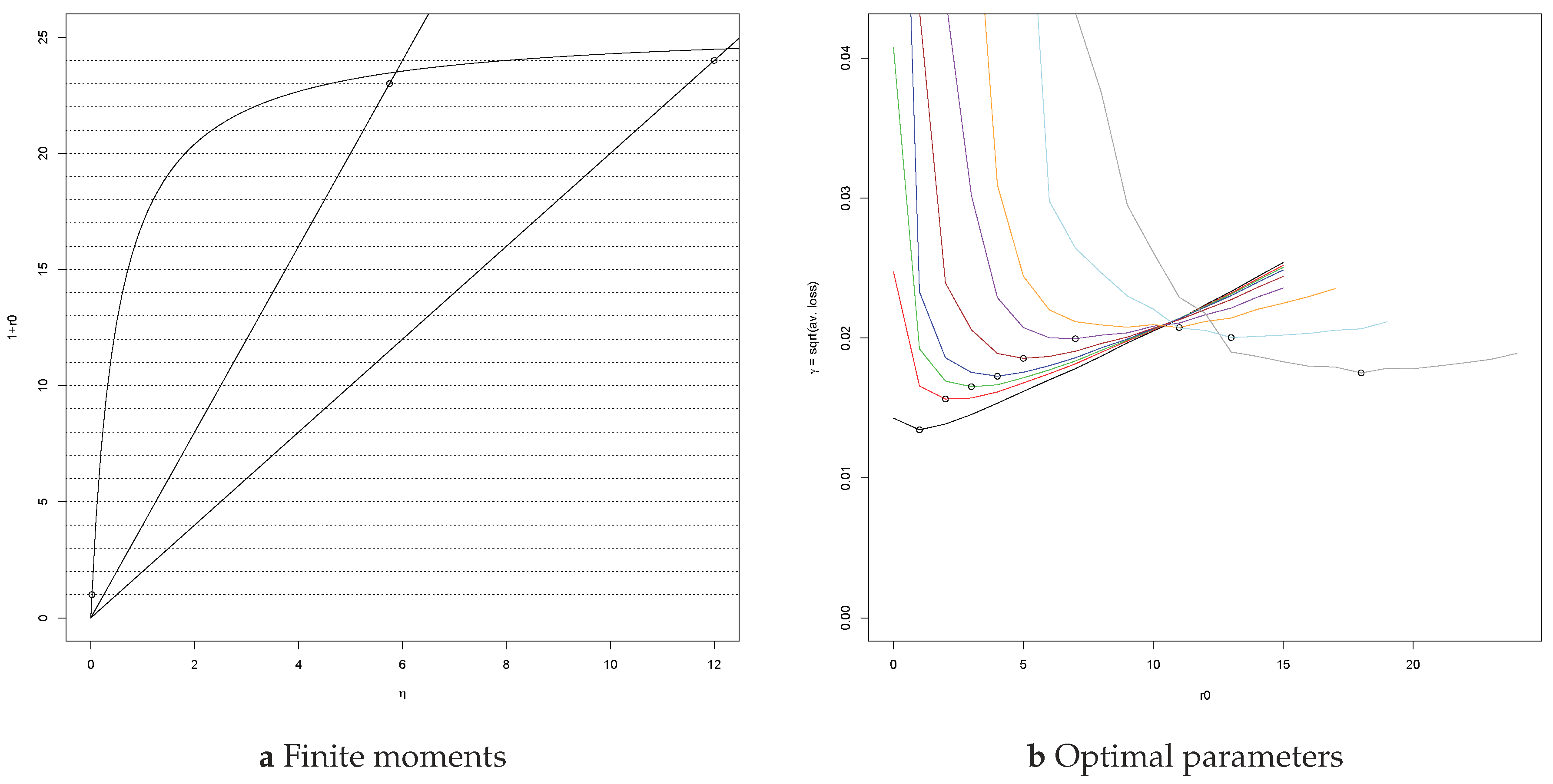
Similarly, is finite for η ∈ (1/49, 23/4) for the RM(r) estimator with r = 2r0 + 1 and r0 = [4η].
Appendix A.3. Tails of
For general weights, the argument has to be adapted. Since we measure performance by the loss function , we are particularly interested in weight sequences for which the slope has finite second moment.
Assume sample size n = 100. Define points with index i < 50 to be heavy and points with indices i > 51 to be light. There is a positive integer bH depending only on the weight w such that for any line of balance the set of 49 points above the line augmented with the heavier point on the line contains at least bH heavy points. The argument is simple. Let L be a bisector which passes through two points. Suppose there are only k heavy points on or above L. Then, the total weight of the 49 points above L together with the rightmost point on L is at most . If k is small the sum may be less than Ω/2. In that case, L cannot be a line of balance and bH > k. Similarly, balance implies that there are at least bL light points on or above the line of balance, and by symmetry also at least bL light points on or below the line. A four line program in R will yield bH as the smallest integer k for which the sum above equals or exceeds Ω/2, as well as for bL. The minimum b = bH ∧ bL is called the balance minimum for the weight w. For the hyperbolic weight , i = 1, …, 100, we obtain the result in Table A1.

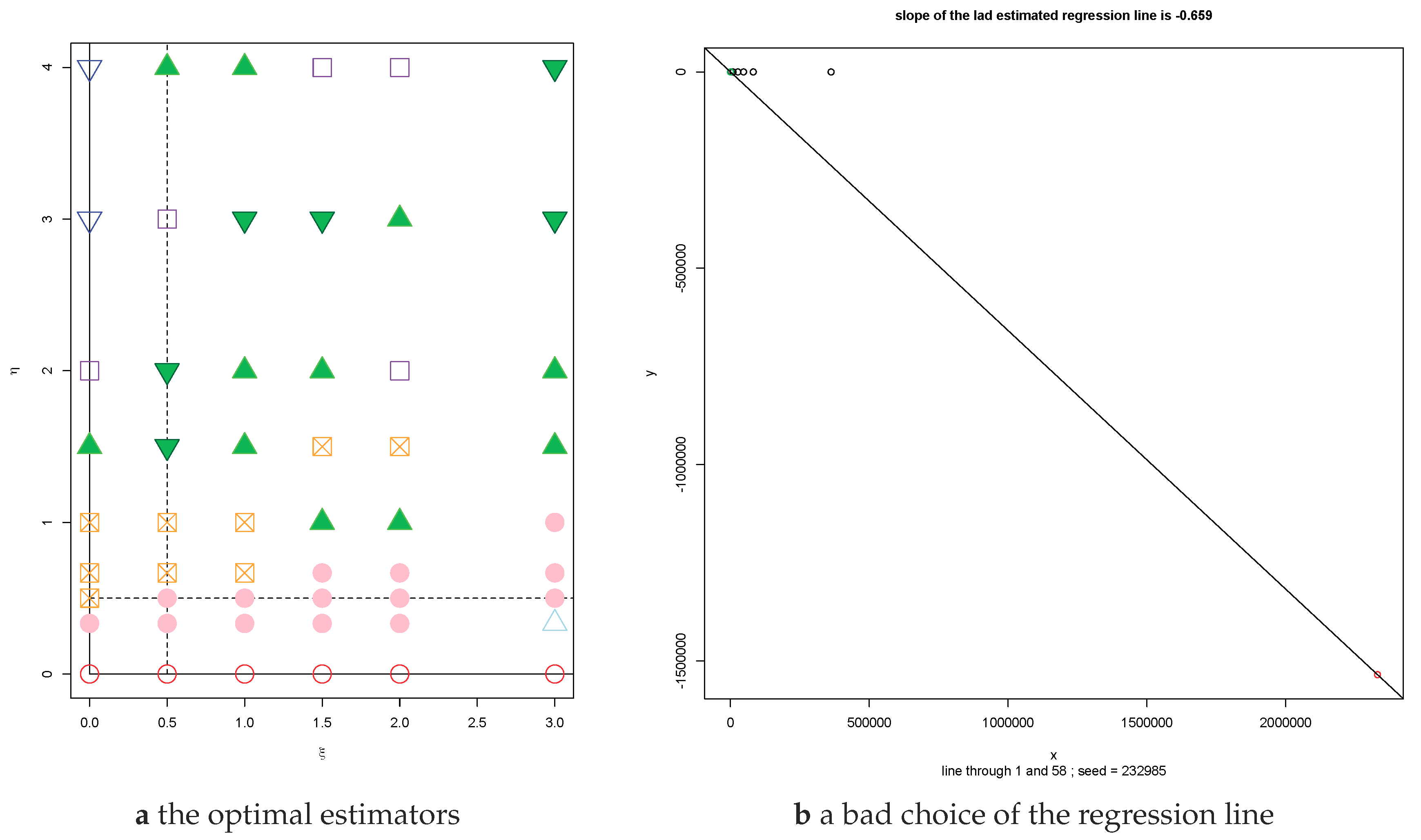
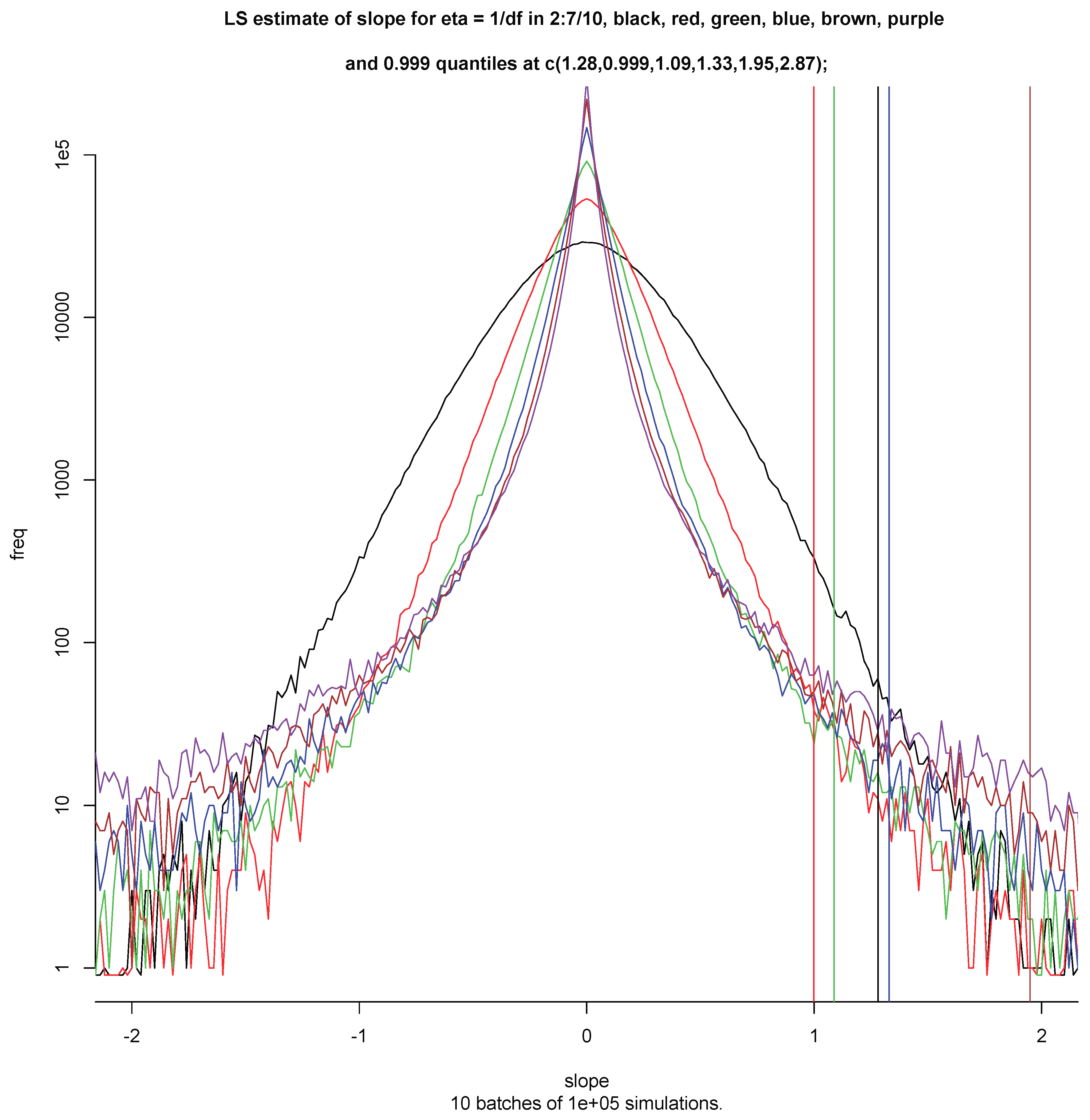
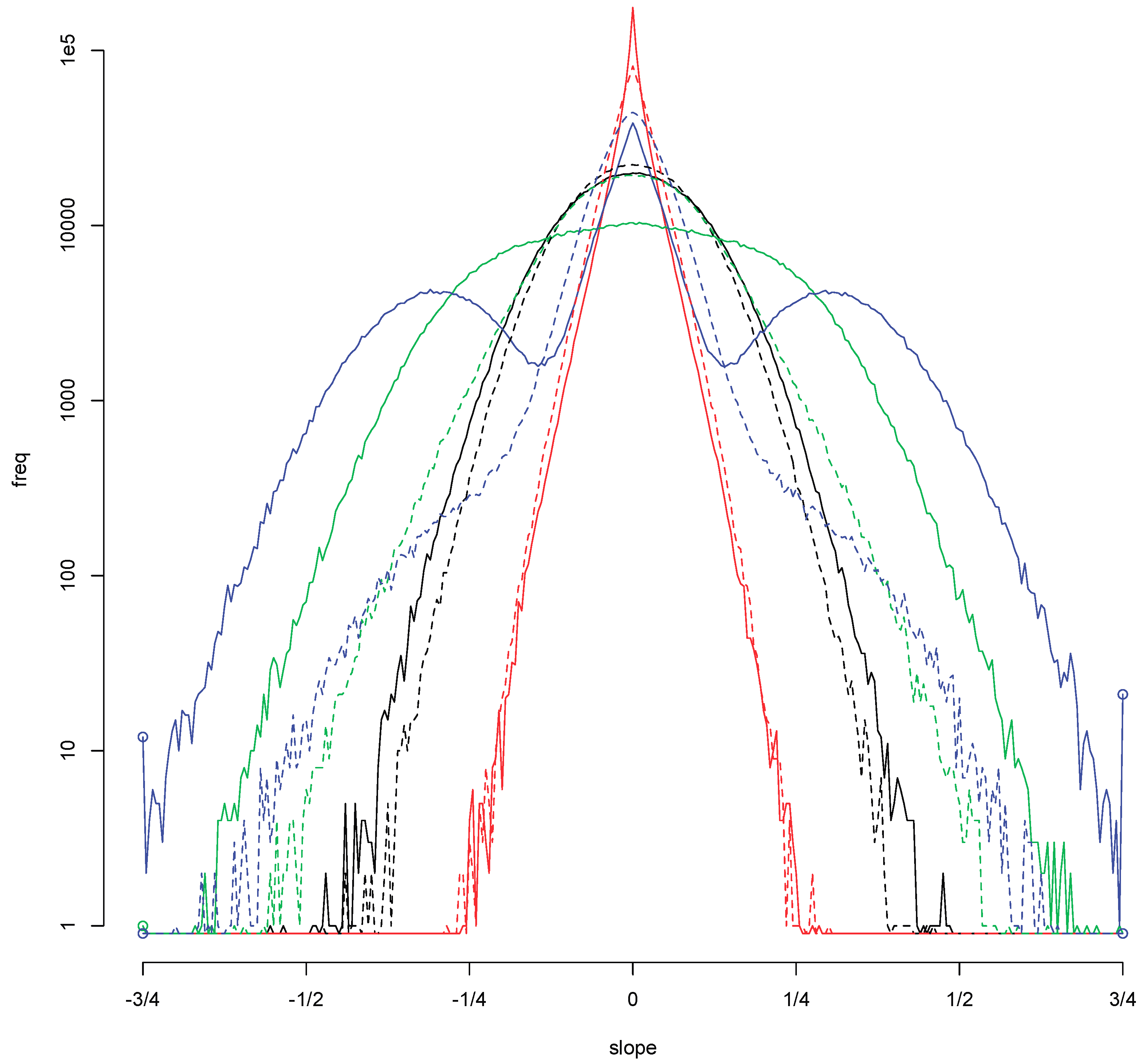
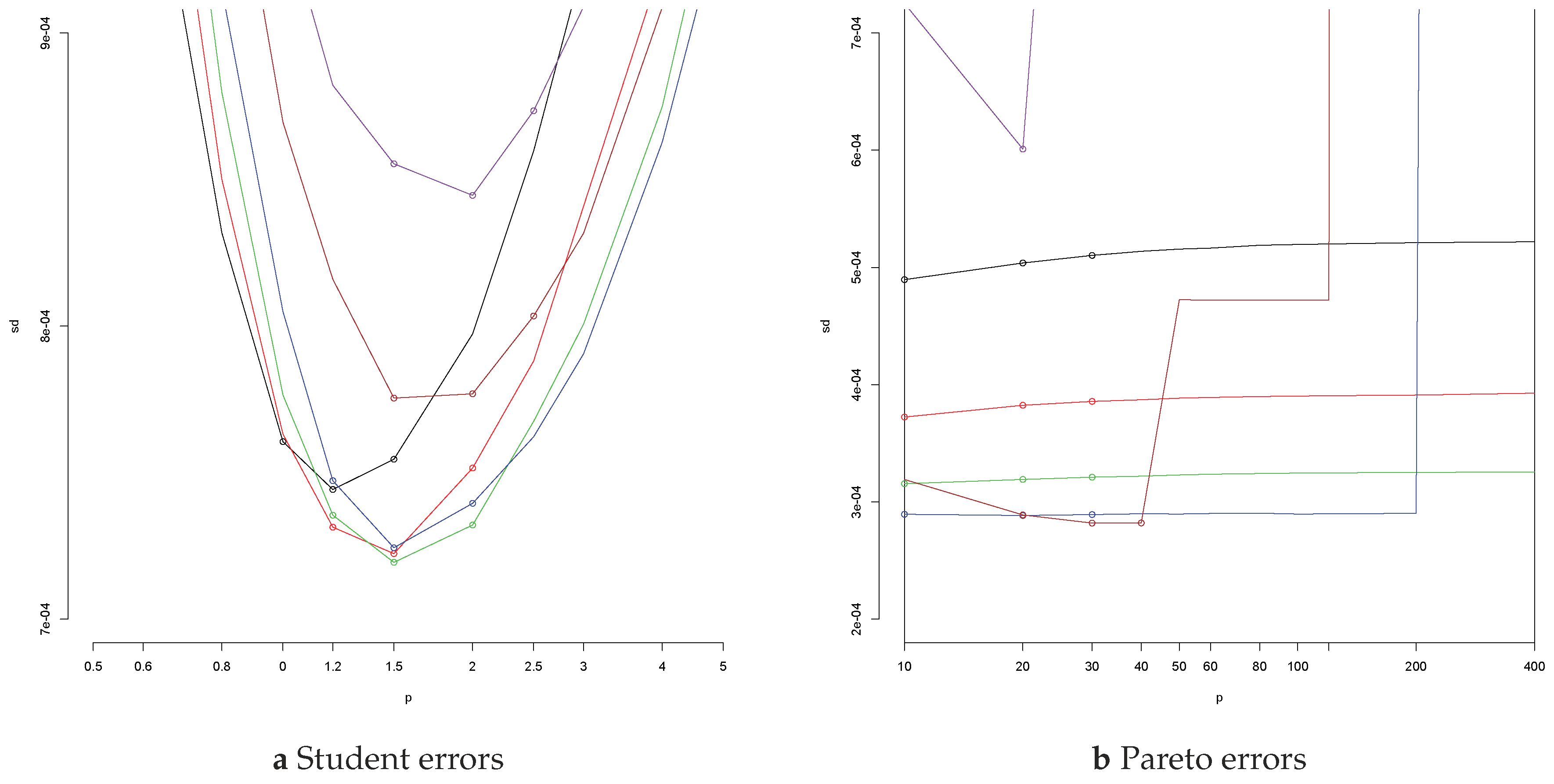
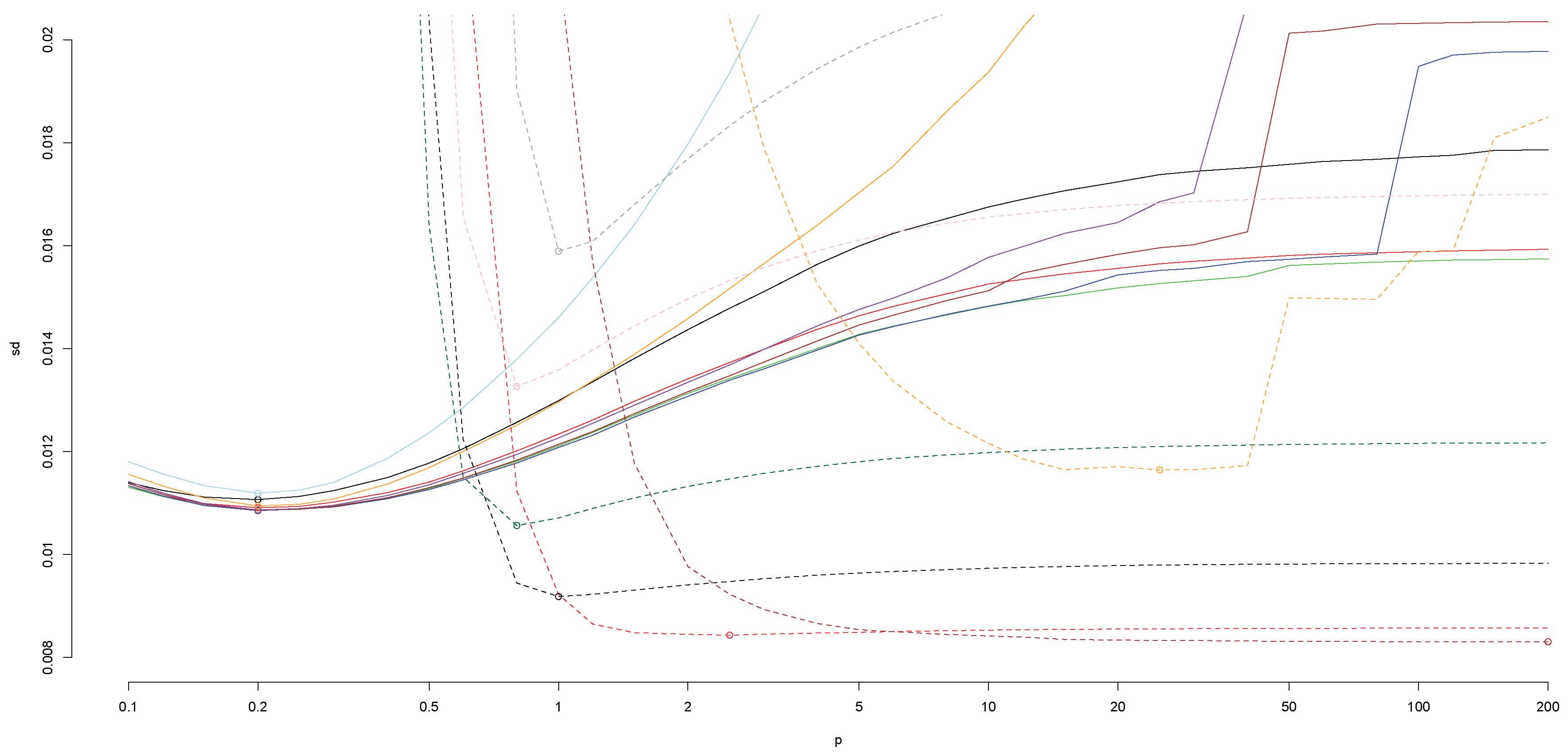
Table A1.
The heavy and light balance minima for HB0(d) for sample size n = 100 and various d.
| d | 1 | 2 | 5 | 10 | 20 | 50 | 100 | 200 | 500 |
| 4 | 6 | 8 | 10 | 12 | 14 | 14 | 15 | 15 | |
| 3 | 5 | 7 | 9 | 11 | 13 | 14 | 14 | 15 |
One can now use the argument which was used for the Right Median in the proposition above. Set D = (X49 − X52)/2. Then, , and for t > 0 the event is included in the union of a finite number of events where J is a subset of {1, …, 49} or of {52, …, 100} containing b elements. This has been done in Balkema (2019). Since the tail index of the error plays an important role in the present paper, we use that to formulate a simple corollary to the theorem.
Proposition A3.
Let the variables X and Y* in the linear regression in Equation (1) have continuous dfs. Suppose the error has tail index and the weight has balance minimum b ≥ 1. The slope of the corresponding WB estimator of the regression line has finite second moment if .
Proposition A4.
Suppose the sample size n = 2m is even. Let w be a weight sequence and define the dual weight w* by . Then, the light balance minimum of w is the heavy balance minimum of w*.
Proof.
For even sample size, the heavy points for w* are the light points for w and vice versa. ☐
Example A1.
For sample size n = 1000 and parameter d = 250, we find bH = bL ≥ 121 for the hyperbolic weight . Hence, the slope of the HB0(d) estimate of the regression line for d = 250 will have finite second moment if X has a Pareto distribution with tail index ξ > 0 and if the error has a continuous df with tail index η ≤ 60.
Example A2.
Assume n = 100. There exist weights with balance minimum b = 0. No weight has balance minimum b > 25. For the weight 1, 0, …, 0 associated with RMP the set A of fifty points with indices i = 2, …, 51 contains no light points, but the weight of A is less than half the total weight. Hence, bL = 0. Suppose b > 25. Then, bL and bH both exceed 25. Hence, any set A of fifty points which contains 25 heavy points has weight < Ω/2 where Ω = ∑wi is the total weight. Now, let A be the set of points with indices . Since w is decreasing and not constant, it follows that w(A) > w(B) where B is the complementary set of fifty points.
Appendix A.4. Tails of
On the one hand, there are tails which are as heavy as the tails of the error, while, on the other hand, there are tails which decrease so fast that there is a finite second moment even when the error has tail index η = 4. How does one harmonize these different tail behaviours for the slope ? There exists a simple technical solution. Before we formulate that, let us remark that one of the attractions of weighted balance estimators is the transparent tail behaviour. One may be unhappy about the heavy tails of LAD and its adapted forms LADPC and LADGC, but the tail behaviour is clear, it has a simple description and the reason for the heavy tails is clear too: For certain configurations, the weight will be close to an affine transformation of the weight (1, 0, …, 0) of RMP and for these configurations the estimator will exhibit the bad tail behaviour of RMP. Similarly, the tail behaviour of RM and HB has a simple explanation: The balance condition implies that there exists a positive integer b, the balance minimum, which depends only on the weight such that for any configuration the line of balance will be steep only if at least b sample points have vertical coordinates which are large in absolute value. For sample size n = 100, the balance minimum of ten ensures that the slope has finite second moment if the tail exponent of the error is less than five.
There is a simple formula for combining the responsiveness of LADGC with the good tail behaviour of HB.
Definition A2.
The Deterministic Correction of the random weight Vi by the deterministic weight wi is the weight Wi which agrees up to a scale factor with the weight Vi in the right half of the points and with the weight wi in the left half. Set Wm = 1 for m = [n/2] and
The Hyperbolic Correction of LAD, LADHC(d) is the deterministic correction of the random sequence Vi of LADGC by the hyperbolic weight wi = 1/(d − 1 + i).
Wi = Vi/Vm i ≤ m; Wi = wi/wm i ≥ m.
In simulations, the gap correction of LAD and the hyperbolic correction (with the same parameter d) are indistinguishable. This only aggravates the problem of the disparity in the tail behaviour. For tail indices (ξ,η) = (2,4), the tail of is bounded below by c/t1/4; the tail of is bounded above by C/t5/2. How does one choose between an estimator with tails of the order of c/t1/4 and one with tails of the order of C/t5/2? To compare the tail behaviour of the gap correction and the hyperbolic correction, one would need to have information on the constants c and C. Sharp bounds on such constants are hard to obtain and will depend not only on the parameters but also on the shape of the underlying dfs. In the absence of such constants, we have to accept the lower bound on the tail of as a weakness of the estimator. A weakness shared by all weighted balance estimators that are responsive to the configuration of the horizontal coordinates of the sample points. One would like to know how many simulations are needed to reveal the flaw. For LAD, a million suffice if the error has very heavy tails, η ≥ 3, even when the tail index of X is small, ξ = 1/4, as shown in Section 3. For LADGC, the flaw is not visible in the simulations analyzed in this paper. It is known for which configurations the estimate will be poor: The rightmost x-coordinate is isolated and the remaining x-coordinates all cluster together. Such configurations pose problems for many estimators. Pivot points have received considerable attention in the statistical literature. The hyperbolic correction solves the estimation problems associated with these configurations. It combines sensitivity to the configuration of the horizontal coordinates in the right half of the sample points with the good tail behaviour of the HB0 estimator, while achieving the same performance as the gap corrected version of LAD.
The weight for LADHC(d) is random. Hence, so is the balance minimum. However, for the deterministic correction of a random weight (Vi) by a deterministic weight (wi), there is a lower bound b0 for the balance minimum which only depends on the sequence (wi). We give the arguments for the heavy balance minimum below for n = 2m. Recall that k < bH holds if a set of m sample points which contains at most k heavy points (with index i < m) has weight less than Ω/2 where Ω is the total weight of all sample points. Maximizing the weight of this set of m sample points gives the inequality
which may be written as
The left hand side is random, the right hand side deterministic.
Proposition A5.
Let W be the deterministic correction of a random weight V by the deterministic weight w for sample size n = 2m. Let Ω = ∑Wi. There exists an integer which depends only on w such that any set A of m sample points which contains less than points with index i < m has weight W(A) < Ω/2. The value is optimal: There exists a weight V0 and a set A0 of m sample points, of which have index i < m, such that W0(A0) ≥ Ω/2 holds with positive probability.
Proof.
Assume that w has been scaled to satisfy wm = 1. Introduce weights z = z(t) for 1 ≤ t ≤ w1 by
Observe that z(1) = w ∧ 1 and z(w1) = w. In general, for t ∈ (w1/wj, w1/wj + 1), the weight z(t) satisfies zi(t) = 1 for i > j and zi(t) > 1 for i = 1, …, j. Let d = d(t) denote the difference D on the right hand side of Equation (A5) for the weight z(t). One can show that t ↦ d(t) is continuous on [1, w1] with a derivative which is constant on intervals (w1/wj, w1/wj + 1), negative on (1, w1/w2k), and increasing on (w1/wk, w1). Hence, d is a piecewise linear convex function on [w1/wk, w1]. It is minimal in w1/wj for an index j ≥ 2k where j = m or j is the first index i for which . Let d0 denote this minimum. Now, observe that conditional on Wk = c ≥ 1 the difference D in Equation (A5) is bounded below by d(t) if we choose t such that zk(t) = c. Hence, D ≥ d(T) ≥ d0 for T = w1Wk/wk. Define to be the minimal integer k for which d0 = d0(k) ≤ δ. If j0 ≥ 2k0 is the index j associated with then the weight V0 = z(t0) with satisfies V0(A) ≥ Ω/2 where A is the set of sample points with index i ∈ {1, …, k0} ∪ {m, …, n − 1 − k0}. ☐
If L is a bisector for the weight W and balance holds, then the set of m − 1 points above L together with the heavier point on L contain at least points with index i > m. One may define the light balance minimum similarly. These two integers depend only on the deterministic weight w. For the hyperbolic weights wi = 1/(d − 1 + i) and sample size n = 100, the optimal lower bounds and for the heavy and light balance minima are listed in Table A2 for various values of the parameter d.
Table A2.
The heavy and light balance minima bH and bL for HB(d) for sample size n = 100 and various values of d and the optimal lower bounds and for the corresponding Hyperbolic Correction of a random weight.
Table A2.
The heavy and light balance minima bH and bL for HB(d) for sample size n = 100 and various values of d and the optimal lower bounds and for the corresponding Hyperbolic Correction of a random weight.
| d | 1 | 2 | 3 | 4 | 5 | 6 | 8 | 10 | 12 | 15 | 20 | 25 | 30 | 40 | 50 | 60 | 80 | 100 |
| 4 | 6 | 7 | 7 | 8 | 9 | 9 | 10 | 11 | 11 | 12 | 12 | 13 | 13 | 14 | 14 | 14 | 14 | |
| 3 | 5 | 5 | 6 | 7 | 7 | 8 | 8 | 9 | 9 | 10 | 10 | 11 | 11 | 11 | 12 | 12 | 12 | |
| 3 | 5 | 6 | 7 | 7 | 8 | 9 | 9 | 10 | 11 | 11 | 12 | 12 | 13 | 13 | 13 | 14 | 14 | |
| 2 | 4 | 5 | 6 | 6 | 7 | 7 | 8 | 8 | 9 | 10 | 10 | 11 | 11 | 11 | 12 | 12 | 12 |
Appendix A.5. The Left Tail of Dn
With a sample of n points, associate the uniform distribution on these n points and the mean m and sd d associated with this distribution. With the sample X1, …, Xn, associate the variables S, Q, V, M, D:
and
Proposition A6.
Let be the average of a sample of size n > 1 from a df F with a bounded density and let D > 0 be the square root of
There exists a constant A = An such that
Proof.
The inequality D2 < s2 implies that the sample clusters around the average M: more than m points Xi satisfy . (If holds for n − m indices then D2 > 2(n − m)s2/n ≥ s2.) Clustering implies that the interval contains more than m points. In terms of the order statistics X(1) < ⋯ < X(n): There exists an index i = 1, …, n − m such that
We first derive bounds on the events Ei(r) = {Ui + m − Ui < r} for uniform order statistics Ui. By symmetry, . The order statistic Uk has density fk,n and
Conditional on Ui = u, the difference Ui + m − u is distributed as (1 − u)V where V is the mth order statistic from a sample of size n − i from the uniform distribution on (0, 1). Hence,
We may restrict attention to i ≤ [([n/2] + 1)/2] + 1 by symmetry. Then, n − i ≥ m and and
Finally, write X = F←(U). Then, and
where ∥f∥∞ is the bound on the density f of X. This yields the desired inequality with , where C is a sum of products . ☐
Appendix B. The Poisson Point Process Model
Recall the alternative model for the regression equation introduced at the end of Section 2. Instead of a sample of n points (Xi, Yi) in the plane with , we look at the n rightmost points of a Poisson point process Na with points (Xi, Yi), . Here, where U1 < U2 < … are the points of the standard Poisson point process on (0, ∞). The tail index ξ is positive. The points X1 > X2 > … then form a Poisson point process on (0, ∞) with mean measure ρ(x, ∞) = 1/xλ for λ = 1/ξ. The iid sequence from the error distribution F* is independent of the Poisson point process (Xi). If F* has density f*, then Na has intensity on . Almost every realization of Na determines the error distribution, as shown below. Hence, the value of the abscissa b in the regression equation is of little interest. The question is: Do the realizations of Na determine a?
If the tail index ξ of ρ exceeds a half and the error has a Student or Gaussian distribution, then Na does not determine a. The distributions πa of the Poisson point processes Na are equivalent. One may write dπ0 = fadπa and dπ0 = gadπa. We explain this more precisely below. We then give conditions on the error distribution which ensure equivalence of the distributions πa, , for ξ > 1/2. Roughly speaking, the density f* of the error Y* should be positive and smooth. We also briefly investigate the influence of irregularities in the error distribution. The second half of this section contains an analysis of the behaviour of the estimate of the slope of the regression line based on the n rightmost points of the Poisson point process N0 for n → ∞ for two estimators: Least Squares and Right Median. For both, one may define . For LS, Figure 3 at the end of Section 2 plots the sd of , 0 ≤ ξ ≤ 3, for various sample sizes, n = 20,50,100,200,500,1000 and for n = ∞. Below, we present similar plots for the empirical sds of the RM(r) estimates for the optimal value of the parameter r. The figures for LS and for RM(r) both suggest convergence for n → ∞. It is shown that convergence holds.
Appendix B.1. Distributions and Densities of Poisson Point Processes
One can distinguish a biased coin from a fair coin by repeated trials. Similarly, one can distinguish a normal variable with variance one and positive mean from a standard normal variable. One can distinguish a Poisson point process on (0, ∞) with intensity c > 1 from the standard Poisson point process. However, what happens if the bias varies over time, if the mean tends to zero and if the intensity is not constant but a function which tends to one? Suppose the Poisson point process on (0, ∞) has intensity j(t) which tends to one for t → ∞. If the difference in the number of points on (0,t] between the Poisson point process with intensity j and the standard Poisson point process is masked by the random fluctuations in the standard point process which are of the order of . Does this imply that one cannot distinguish samples from the two point processes?
To answer this question, one has to look at the distributions. If the probability measures which describe the distributions of the point processes are singular, one can distinguish samples with certainty; if the distributions are equivalent, one cannot.
Densities of random variables or vectors are generally taken with respect to Lebesgue measure. One can also consider the density of a variable X with respect to a standard variable U. If X is N(c, 1) and U is N(0, 1) the density of X with respect to U is f(U) = Z/C where Z = ecU and . If (Xn) is a sequence of independent N(cn, 1) variables with mean cn = 1/n and (Un) are independent standard normal variables, the density of the sequence X with respect to the sequence U is f(U) = Z/C where and . The Monotone Convergence Theorem applied to shows that . Samples from (Xn) and from (Un) cannot be distinguished with certainty. Our aim is to show that this also is the case for samples from the Poisson point processes Na on for ξ > 1/2 if the error Y* has a Student distribution.
The situation is not quite symmetric. If the density of X with respect to U is f(U), then the density of U with respect to X is g(X) where g = 1/f, but only if f is U-a.s. positive. Thus, if the intensity j of the Poisson point process Nj on (0, ∞) vanishes on the interval (0, 1) a sample which has a point in this interval evidently derives from the standard Poisson point process on (0, ∞) and not from Nj. We now consider Poisson point processes N and M on a separable metric space with mean measures ν and μ. Assume dν = gdμ with g = eγ.
Theorem A3.
Let M be a Ppp on a separable metric space E with mean measure μ and N the Ppp with mean measure gdμ for g = eγ. The distribution of N has a density h(M) with respect to the distribution of M in the following situations:
- μE < ∞ and g ≡ 0: ;
- μE < ∞, g = eγ > 0, ∫gdμ < ∞: ;
- g = eγ > 0, ∫γ2dμ < ∞, ∫|g − 1 − γ|dμ < ∞: .
Proof.
If K and K0 are Poisson variables with expectation c,c0, the density of K with respect to K0 is Z/C where and . Note the similarity with the normal variables. Poisson and normal both are exponential families. Let for disjoint subsets E1, …, Em of E and dν = gdμ. Set and . Then, the density of N with respect to M is Z/C where
and . The extension to positive μ-integrable Borel functions g is standard, and so is the L2 extension if μE = ∞. ☐
The Poisson point process Na on has intensity for λ = 1/ξ where f* is the error density. We are interested in the density Z/C of Na with respect to N0. The restrictions of the intensities to the half plane {x ≥ 1} are probability densities. If f* is strictly positive the restrictions of Na have equivalent distributions by the second condition above. This is not surprising. One can hardly expect to determine with certainty the slope of the regression line from the few points if any of Na in this half plane. However, what if one knows the position of all points?
First, observe that for any ξ > 0 almost every realization of N0 determines the error distribution. Recall that for the standard Poisson point process N on (0,∞) the number Nt = N(0,t) of points of N in the interval (0,t) is almost surely asymptotic to t for t → ∞. Indeed, the Law of the Iterated Logarithm applies:
Let N0(x) denote the number of points of N0 in the half plane , and N0(x,y) the number in . Assume F* is continuous in y. Then, N0(x,y)/N0(x) → F*(y) a.s. for x → 0+. This also holds for Na. If F* is continuous, the limit relation holds almost surely for all rational y and for all integers a. Hence, there is a null set Ω0 such that
Appendix B.2. Equivalence of the Distributions πa for ξ > 1/2
For many smooth strictly positive error densities for ξ > 1/2, almost no realization of Na determines a. The distributions of Na, , are equivalent. Since equivalence holds for the restrictions of Na to {x > 1} for positive error densities f* it suffices to prove equivalence for the restrictions of Na to the vertical strip . We apply the third criterion of the theorem above with M = N0 and N = Na. Then, g = eγ> with γ(x,y) = φ(y) − φ(y − ax). Set Δ(y) = φ(y) − φ(y − t). If we can prove that and are O(t2) for t → 0+, the two integrals ∫γ2dμ and ∫|g − 1 − γ|dμ are finite for ξ > 1/2 and dπa = hdπa. By symmetry, the distributions πa of all the point processes Na are equivalent.
We formulate simple criteria on the error density which ensure that the distributions of the point processes Na are equivalent. The basic condition is that is strictly positive and continuous and that φ is the integral of a function which is bounded on bounded intervals. The function need not be continuous. If is bounded, equivalence holds. If tends to ∞ for y → ∞ or to −∞ for y → −∞, extra conditions are needed. We then assume a second derivative which is bounded on bounded intervals and which satisfies some extra conditions.
Set Δ(y) = φ(y) − φ(y − t) where . We consider the two integrals
We want to show that the two integrals are O(t2) for t → 0. Write for the integral over the interval (a,b).
Proposition A7.
Suppose φ is the integral of a bounded function . Then, J(0) and J(1) are O(t2) for and the distributions , , are equivalent for ξ > 1/2.
Proof.
Let . There exists a constant C such that . Hence, it suffices to prove that is . This follows since where is a bound for . ☐
The set of densities described in Proposition A7 is closed for shifts, scaling, reflection, exponential tilting and powers. If satisfies the conditions, then so do , for , , provided the mgf is finite at , and for provided the integral of the power is finite.
If the density is logconcave, is increasing. If the limits at ±∞ are finite the distributions, are equivalent. This is the case for Laplace densities with , and for the EGBP densities. If the derivative of varies regularly at ∞ with exponent , then and the distributions of the Poisson point processes are equivalent for ξ > 1/2. Student densities satisfy the conditions of Proposition A7, and so do the continuous unimodal Pareto densities
For the normal density, is not bounded. The situation then is less simple. We assume that is locally bounded. The integrals and are for bounded intervals . We introduce extra conditions on the behaviour of φ at +∞ which ensure that the integrals over (b, ∞) are O(t2) too. Results for the left tail are similar.
First, note that , and . Write
The first integral equals by the remarks above and the second is bounded by since on (0, ∞). Hence, it suffices to give conditions which ensure that J(0) is O(t2) for t → 0 and also .
Proposition A8.
Suppose is continuous and is the integral of . Assume is bounded. Assume is bounded on [0, ∞) or for y → ∞, and similarly for on . Then, and are for and the distributions of the Poisson point processes , , are equivalent for ξ > 1/2.
Proof.
Let C be a bound for . Then, . This shows that J(2) is O(t2). For any , the integral J(0) over the interval is O(t2). Thus, consider the integral over (c, ∞). If is bounded the proof of the previous proposition applies. Thus, assume for y → ∞. Observe that and that uniformly on bounded t-intervals since is bounded. Hence, for y → ∞ and and also . It follows that for , and for b sufficiently large
A similar argument works for the integral over . ☐
Proposition A9.
Suppose is continuous and is the integral of a locally bounded function . Assume for y → ∞ and uniformly on bounded t-intervals. There exists a constant b such that the integrals and are .
Proof.
Observe that and that and that uniformly on bounded t intervals, and similarly , and uniformly on bounded t-intervals for y → ∞. Hence, by the same argument as above. For , we find . Now, observe that implies . ☐
The last proposition shows that for errors with positive smooth Weibull densities the Poisson point processes are equivalent. A Weibull density has tail for positive, or more generally for a function R which varies regularly with exponent . Here, we need to assume that varies regularly. The exponents for the left and right tails may differ. The density of the double exponential Gumbel distribution is logconcave but increases too fast for the conditions of the propositions above to apply.
Appendix B.3. Error Densities with Local Irregularities
For errors with a Student or Gaussian distribution and ξ > 1/2 no realization of Na determines a. Sometimes local irregularities in the error distribution may help to determine a. For errors with a Pareto distribution and , almost every realization of Na determines a. We look at the effect of irregularities below.
Lines L with slope a through , where is a discontinuity of the df , contain infinitely many points of Na almost surely. With probability one, no other line contains more than two points. For discontinuous error distributions, Na determines a almost surely, whatever the value of ξ > 0.
Henceforth, we again assume a continuous error distribution. There may still be local irregularities in the density which reflect in the Poisson point process Na. The density may have a zero or become infinite at some point. It may have a jump, a vertex or a cusp. It may vanish on an interval or a half line.
The exponential density and shifted Pareto densities are positive on [0, ∞) and vanish on . The points of Na lie above the ray with slope a. For certain values of the tail index ξ, this boundary is sharp. The sector bounded by the horizontal axis and the ray with slope has mean measure
Since for and we see that for all for .
Proposition A10.
Let the error distribution have a finite lower endpoint and suppose for for a constant . Then, determines a almost surely for : a is the maximal slope for which there are no points of Na below the line .
A similar argument shows that Na determines a almost surely for if the error has a Gamma distribution with shape parameter .
If has an irregularity at the origin, it is the restriction of the point process to sectors bounded by two rays with slope which determine whether one can distinguish the point processes Na. Assume
For , the mean measure of the sector is infinite since for . Let denote the mean measure of the truncated sector . For ,
where for and for . For , the limit is . The limit relation holds almost surely if one replaces by Na. Hence, if one can distinguish the functions , one can distinguish the point processes Na almost surely for . The functions Ha can be distinguished unless and . Then, has a positive derivative at the origin:
Proposition A11.
Let the df of the error satisfy Equation (A12). Then, Na determines a almost surely for unless and .
In particular, Na determines a almost surely for if the error density has a jump.
Appendix B.4. Two Plots
The two figures in Figure A2 give a good description of the performance in two specific situations: Least Squares for Gaussian errors in the upper figure and Right Median for Cauchy errors in the lower figure.
We consider estimates of the slope of the regression line based on the rightmost points of the Poisson point process and estimates of the slope of the regression ray . For , the Poisson point process has intensity , . For , the intensity is adapted as described in the caption in order to ensure continuity at ξ = 0 for the estimates . For ξ = 0 the intensity is on .
The sd depends on the error distribution and on the estimator. In the upper figure, we plot and for the Least Squares estimator with Gaussian errors scaled to have IQD = 1; in the lower figure, the errors have a Cauchy distribution scaled by its IQD and the Right Median estimator with parameter r is used. Here, r is an odd integer, the number of “red” points. It depends on n and ξ and is chosen to yield the minimal average loss over a million simulations. The curves plot the empirical sd, the square root of the average loss over a million simulations.
The similarity between the two figures is striking. For sample size n = 20,50,100,200,500,1000, the full curves form a decreasing sequence, as do the dotted curves. These lie below the full curves. Knowledge of the abscissa gives a substantial improvement of the estimate. For , the full black curve, , can scarcely be distinguished from the purple dotted curve . This is not a defect of the estimators LS and RM. For ξ large, the points of the explanatory variable tend to zero so fast that the value of for is of little use in estimating the slope of the regression line. For ξ closer to 1/2, we see the same phenomenon in a less extreme form. For ξ > 1/2, the asymptotics of and for n → ∞ is trivial. Convergence to a positive limit holds without any normalization. That also is the case for the distribution of and . Details are given below.
For ξ > 1/2, we could have listed in Section 7 the empirical sd for n = ∞ rather than n = 100. There are practical drawbacks. It is not always clear how the limit variable, the estimate should be defined. For HB0 and HB40 one can show that truncation of the weight at an appropriate index hardly affects the performance, and one may define for the truncated weights. For LAD and the variations LADPC and LADHC, or for Theil’s weighted estimator or Weighted Least Trimmed Squares, or the estimators TB1, TB2 and TB∞, it is not clear how the empirical sd for sample size n = ∞ should be determined. Since the intention of the paper is to introduce and describe a number of estimators which perform well for heavy tails, the focus on the finite sample size n = 100 is a viable procedure. In principle, it makes no difference whether one takes n = 100 or n = ∞ as the standard.
Figure A2.
The upper figure shows the sd of the slopes , , (and , , dotted) of the LS estimates of the regression line y = ax + b (and the regression ray y = ax) for the n = 20,50,100,200,500,1000 (azure, pink, black, red, green, blue) and ∞ (purple dotted) rightmost points of the Poisson point process for normal errors with IQD = 1. The sds have been scaled by . The lower figure shows the scaled empirical sd for the RM-estimates for errors with a Cauchy distribution scaled by its IQD, based on a million simulations. In both figures, the explanatory variables have the form for where are the points of the standard Poisson point process on (0, ∞). For for ξ = 0 and for 0 < ξ < 1. For , for 0 < ξ < 1. This renormalization is standard in extreme value theory. Because of the geometric nature of the estimators the effect on , and on , is simple. The values for the sequence are multiplied by ξ to obtain the values plotted in the figure above. The extra factor ξ on (0,1) explains the kink in the curves at ξ = 1. This is the price we pay for continuity of and at ξ = 0.

A closer look reveals several differences between the upper and lower figure. The curves for LS are lower than the corresponding curves for RM. The decrease over the interval [1,3] is stronger for LS. The dotted lower curves for RM vanish when ξ becomes large. The dotted purple curve for LS seems to decrease to zero for ξ → 1/2 + 0. This behaviour is less marked for RM. Some of these differences have a simple explanation. LS is optimal for normal errors, the performance of RM is only fair for Cauchy errors. The estimator RM has been chosen not for its good performance but because of its intuitive simplicity and because its behaviour for n → ∞ and for n = ∞ can be described by simulations. The estimate for RM(r) has a simple form. Draw the rays through the rightmost points of . Then, is the median of the slopes of the r rays. If ξ is large, r is small since one wants to make optimal use of the leverage effect of the largest values of X in the estimate of the slope. The slow rate of decrease of and over the interval for RM is due to the heavy tails of the Cauchy error. Heavy tails of Y* demand a conservative estimator. For ξ > 2, RM is the median of the slopes of the rays through the r = 5 or r = 7 rightmost points of . It does not exploit the leverage effect of the rightmost point to the full. The dotted curves for for n = 20,50,100,200,500,1000 coincide with the purple dotted curve for if ξ is so large that the optimal value of the parameter r for is less than twenty.
It should be pointed out that IQD is a good normalization if one wants to compare errors with different tail indices η, but an unnatural normalization for LS. One can construct bounded errors Y* with IQD = 1 and with a symmetric unimodal density for which the sd is very large. A normal error scaled by its IQD has sd 0.74. If one takes a bounded error Y* with IQD = 1 and sd = 1.5, the curves in the upper figure will all be shifted upwards over the same distance, corresponding to an increase in the sds by a factor two.
The plots in the lower figure are random. They depend on the seed with which we start our sequence of a million simulations. This randomness is more pronounced for large values of ξ where r is small. It may account for the anomalous behaviour of the dotted purple curve for ξ → 3.
Appendix B.5. Convergence for the LS Estimates
If the explanatory variables have finite second moment, the Least Squares estimators and are consistent Drygas (1976) and asymptotically normal (see Kuan (2007)). Figure A2 suggests that vanishes on (0,1/2] and is positive on (1/2,3], and that and converge to for n → ∞. We prove this and show that and converge almost surely to for ξ > 1/2. For , convergence in distribution was established in a more general setting in Samorodnitsky et al. (2007).
The sd dn of the slope of the LS estimate of the regression line is and the sd of the slope of the LS regression ray is , where
with Mn the mean of X1, …, Xn. Here, are the points of a Poisson point process on (0, ∞) with mean measure , . We prove that dn and decrease to the same positive limit for ξ > 1/2. The variables 1/Vn and 1/Qn converge monotonically and in to the same finite positive limit for ξ > 1/2. The variables Vn and Qn converge monotonically and in to the finite positive limit . The equation then implies that vanishes in for n → ∞.
For a finite sequence of real numbers , set where
We do not assume that the ti are ordered.
Lemma A1.
Replacing ti by ti − c for has no influence on vn.
Lemma A2.
The sequence vm, , is increasing.
Proof.
Let and set . Assume , see Lemma A1. Then, since . ☐
Write where are the points of a standard Poisson point process on (0, ∞). Then, almost surely and
Lemma A3.
is finite.
Proof.
First, observe that by Lemma A1. Write , where W is Gamma(3) and independent of the standard exponential variable U. Now, observe
Hence, and on and on . Since , the expectation of is finite and so are and . ☐
Similar arguments show that is infinite.
The series is almost surely finite for ξ > 1/2. It may be expressed as where N is the standard Poisson point process on (0, ∞). Write this as where is finite as the sum of the squares with , and .
Proposition A12.
For ξ > 1/2, the variable is almost surely positive and finite. Its expectation is finite and in .
Proposition A13.
For ξ > 1/2, the variable is almost surely finite and positive. Its expectation is finite and in .
Proof.
The inequalities prove that V∞ is finite and positive a.s. Then, Vn ↑ V∞, together with imply convergence in by dominated convergence. ☐
Lemma A4.
V∞ = Q∞ for ξ > 1/2.
Proof.
We have to prove that in probability. Set where is the sum of the terms . Then, almost surely. Now, may be compared to a stochastic integral. Set , where N is the standard Poisson point process on (0, ∞). Then, for
Hence, in . The nth point has a Gamma distribution. Hence, and on . It follows that in probability if . If ξ increases, then decreases for . Hence, for ξ > 3/4 and hence in probability for ξ > 3/4. ☐
Corollary A1.
Suppose ξ > 1/2. Then, in .
Proof.
and converge in and the limits agree. ☐
For ξ = 1/2, the second moment of is infinite. The conditions for consistency of the estimators and in Drygas (1976) do not apply. We prove that and vanish almost surely for n → ∞. The same arguments work for ξ < 1/2.
Proposition A14.
Suppose is centred and has finite variance. Let for ξ = 1/2. The sds and vanish for n → ∞.
Proof.
Introduce the random integrals where N is the standard Poisson point process on (0, ∞) with points . Similarly, we define and . We also consider integrals and over intervals . Set ξ = 1/2. Note that and . The variance of is . Since is a finite sum of variables , we see that . Hence, and by monotonicity , which implies and Dominated convergence by Lemma A3 implies . Similarly, implies . Set . Then, and, as above, . ☐
We now turn to convergence of the estimators and for ξ > 1/2.
Suppose ξ > 1/2. The estimate for the slope of the regression ray based on the n rightmost points with has the form with and as defined in (A13). We assume that is centred normal scaled by its IQD. The series converges in and almost surely if is finite. Hence,
Then, almost surely implies almost surely, hence in distribution. A more general result on convergence in distribution is given in Samorodnitsky et al. (2007). The authors observe that the limit distribution may be expressed in terms of the points of the standard Poisson point process on (0, ∞) as
It is almost sure the equality holds if one expresses the explanatory variables as .
The same limit distribution holds for the estimate where and for the mean of . Set . Then, implies Now, observe that since in by Corollary A1 and converges in distribution to a normal variable. For ξ > 1/2:
Theorem A4.
Let denote the points of the standard Poisson point process on (0, ∞) and let be an iid sequence of centred variables with finite second moment which is independent of the Poisson point process. Let denote the slope of the LS estimate of the regression line for the points where , 1/λ = ξ > 1/2. Then,
Appendix B.6. Convergence for the RM Estimates
The results for the Right Median estimator are slightly different and less complete than for Least Squares.
Recall the limit relation in Equation (A10), rλN0{x > r, y ≤ y0 + ax} → F*(y0), r → 0+. Call a realization of N0 unexceptional if no four points lie on two parallel lines and if the limit relation holds for all y0 and a. At the end of Section B.1, we show that almost every realization of N0 is unexceptional.
Assume F*(0) = 1/2 and the median is unique. Given a weight, a decreasing sequence wi ≥ 0 with finite sum Ω, a ray of balance for an unexceptional realization is a ray L:y = ax such that the weight of the points below L does not exceed Ω/2 and neither does the weight of the points above L. Exact balance holds if one of these sets has weight Ω/2. One of the attractive features of the weighted balance estimators is the possibility to define estimators not only for a finite set of rightmost points of the point process N0 but for the set of all points. The line of balance Ln based on the n rightmost points depends on the weight wn. For the Right Median estimator for ξ > 1/2, simulations suggest that there exists an optimal value r = 2r0 + 1 depending on ξ such that the slope of the ray which divides these rightmost r (red) points fairly has minimal average loss. For the hyperbolic weights for fixed parameter d and ξ > 1/2 there also exists such an optimal truncation. For truncated weights, there is a simple continuity result.
Proposition A15.
Let wn be weights of total weight Ωn and suppose there exists an index r such that the components wni vanish for i > r. Assume wn → w, where w has the property that no subset A of {1, …, r} has weight w(A) = Ω/2 where Ω is the total weight of w. Consider an unexceptional realization N0(ω). Let Ln be a line of balance for the rightmost n points of N0(ω). Assume the df of the error satisfies F*(0) = 1/2 and the median is unique. Then, Ln converges to the line of balance L0 through the origin for the weight w.
Proof.
Let L0 pass through the point z0 of the unexceptional realization N0(ω). We claim that almost all lines Ln pass through z0. This implies Ln → L0 by Equation (A9). The weights w1 ≥ ⋯ ≥ wr ≥ 0 with total weight Ω = 1 for which there is a subset A in {1, …, r} of weight 1/2 lie in a finite union of hyperplanes in . Hence, there exists an index n0 such that for the weights wn, n ≥ n0, no such subset A exists. For these weights, the line of balance is unique. Colour the r rightmost points red. There is an interval such that for y ∈ J the line through (y,0) and z0 divides the red points fairly with respect to the eight w. This then also holds with respect to the weights wn for n ≥ n1. Let L be a line through (0,y) for y ∈ J and assume z0 lies below L. Then, by monotonicity, L does not divide the red points fairly for wn for any n ≥ n1. So too if z0 lies above L. ☐
For ξ < 1/2, the RM estimate based on the n rightmost points of the Poisson point process Na is consistent if the error has a density which is continuous and positive in the median.
Proposition A16.
Assume . Let denote the median of the slopes of the rays through the rightmost n points of the point process Na. If has a density which is positive and continuous at the origin and with , then almost surely.
Proof.
We may assume that a = 0. Set λ = 1/ξ. If there exists and δ0 ∈ (0,1) such that the truncated sector satisfies
then, by the Law of the Iterated Logarithm, for almost every realization of N0, the number of points below the ray through (1,θ) will eventually exceed the number of points above the ray, and hence where is the median of the slopes over the points in . Now, observe that . Since for x → 0+ we find
If n is odd, the ray with the median slope will pass through a point and Kn → ∞ almost surely since is non-zero for i = 1, 2, …. The leverage effect of the horizontal coordinate decreases as Kn increases. Convergence is slow, as shown in Figure A2.
Remark A1.
If has a symmetric Pareto distribution with density on the complement of (−1,1), the df of the RM estimate will converge to the defective df G ≡ 1/2.
Proposition A17.
Suppose almost surely. Then, the empirical sds for the estimates based on a million simulations converge almost surely to the empirical sds of the estimates .
Proof.
The average of a finite number of variables which converge almost surely converges almost surely to the average of the limit variables. ☐
Corollary A2.
For ξ > 1/2, the empirical sds for the RM estimates converge: . Similarly, almost surely. For 0 < ξ < 1/2, almost surely.
Appendix C. The EGBP Distributions
EGBP is the acronym of Exponential Generalized Beta Prime. The EGBP densities form a four-dimensional family of logconcave functions where ψ is a smooth function with asymptotes which have finite non-zero slope. We are interested in the class EGBP since the characteristic shape of the loglog frequency plots of for many estimators E is a concave function with non-zero asymptotic slopes. The fit with a function of the form is good.
There is a relation with heavy tailed distributions on (0, ∞) such as the Gamma distributions and the Snedecor F-distributions and with symmetric heavy-tailed distributions such as the Student distributions. The variable has an EGBP distribution precisely if has a Generalized Beta Prime distribution. A Beta Prime distribution is a Beta distribution transformed to live on the positive half line rather than the interval (0,1). If U has a Beta distribution on (0,1) with parameters a,b, then lives on the positive half line. It has a strictly positive density and its df has tails which decrease like at ∞ and like at zero.
We first give a description of the class EGBP, then show the relation with heavy tailed distributions, and finally discuss the remarkable fit to the loglog frequency plots of the estimators considered in this paper.
Appendix C.1. The Exponential Generalized Beta Prime Densities
This section contains information about EGBP, the set of Exponential Generalized Beta Prime distributions, their densities, the role of exponential tilting, and powers.
We begin with a simple result on logconcave densities . Let denote the derivative of . It is increasing since is convex. We may assume that it is right-continuous. The derivative determines the logconcave density f. If is convex with derivative one may write where is the constant which ensures that . This results in a one to one correspondence between the class LCA of logconcave densities with non-zero finite asymptotes on the one hand and a product space on the other
where DF is the space of all dfs on . Write with p ∈ (0,1) and for some df H. Every non-degenerate df H generates a four parameter family of log concave densities where
LCA ↔ (0,1) × (0,∞) × DF
These families are disjoint unless and are of the same type, in which case the families coincide. The degenerate distribution H concentrated at generates the three parameter family of shifted Laplace densities where
An increasing function which assumes both positive and negative values has a unique primitive such that is a probability density. The probability density associated with is . The probability densities associated with , , are powers . The probability densities associated with for form the exponential family generated by . EGBP is the four-dimensional set of distributions with logconcave densities generated by the logistic df , as we show presently. Here we want to stress that, in terms of the derivative , the four parameters consist of two parameters which determine an affine transformation on the vertical axis and two parameters which determine an affine transformation on the horizontal axis. This holds for any df H by Equation (A16). To describe the four-dimensional class of functions associated with the df , we may use the group of transformations (see Equation (5)).
Example A3.
Note that the density is logconcave, and
The variable S with density is EGBP. The variable has density . We see that and X is the absolute value of a standard Cauchy variable. The question which interests us is whether the loglog frequency plot of for a given estimator E can be approximated well by the graph of , for appropriate constants and .
The density in the example above generates the class EGBP. Every density f in EGBP has the form where with and to ensure that is positive at ∞ and negative at −∞. We now first look at the distributions of the heavy tailed positive variables associated with the variable S with an EGBP density.
Figure A3.
The convex functions for p = 0.5, 0.4, 0.3, 0.2, 0.1, 0 (black, red, green, blue, azure, purple) and the asymptotes for p = 1/2 and p = 0.1.
Figure A3.
The convex functions for p = 0.5, 0.4, 0.3, 0.2, 0.1, 0 (black, red, green, blue, azure, purple) and the asymptotes for p = 1/2 and p = 0.1.

Appendix C.2. Basic Formulas
The Beta Prime distribution with parameters (a,b) has density
The distribution has power tails with exponent a at zero and at infinity. If X has a Beta Prime distribution on (0, ∞), then has a Beta distribution on with the same parameters. The variable X may also be written as the quotient of two independent Gamma variables where has density . The variable yields the power tail of X at zero, the heavy tailed variable the power tail at infinity.
The variable has density
The moment generating function of T has a simple form:
We compute the density and mgf of the normalized variable
Proposition A18.
The normalized variable S above has density and mgf given by
Proof.
Set . Then,
and, hence,
with . ☐
The functions satisfy the symmetry relation:
Let , , be one of the families:
Theorem A5.
Let for one of the three families , , above. The distributions with logconcave densities of the form where
are the EGBP-distributions.
Corollary A3.
EGBP is the set of dfs with logconcave densities of the form where
for the logistic df .
Appendix C.3. The Closure of EGBP
The EGBP distributions form a four-dimensional set in the space of all non-degenerate dfs on with the topology of weak convergence. The closure of this set contains the normal distributions, the exponential and the Laplace distributions, but also the Gumbel distribution for maxima and the corresponding limit distribution for minima. We show that there is a closed triangle of dfs such that EGBP distributions are the dfs where are interior points of the triangle. We first consider the effect of scaling, both in the horizontal and in the vertical direction, on the convex functions .
- Zoom out. The transforms have the same asymptotic slopes as . For , the functions converge to the wedge corresponding to the Laplace density .
- Zoom in. The transforms have the same curvature as at the origin. For , we obtain the parabola corresponding to the standard normal density.
Loosely speaking, the EGBP distributions form a bridge between the normal distributions and the (shifted asymmetric) Laplace distributions.
The density tends to for . The limits and exist. They correspond to the Gumbel distribution and the corresponding limit law for minima. Three limit relations follow from the corresponding limit relations for the derivatives:
- for ;
- for , ; and
- for cn → ∞, pn ∈ (0,1).
Theorem A6.
The closure of this four-dimensional set of EGBP-dfs in the space of non-degenerate dfs is the set of dfs
where Θ denotes the closed triangle with vertices (0,0) and (±1,1) and denotes the df with density for and .
Proof.
Let for r > 0 and p ∈ [0,1]. If (rn,pn) → (0,0) and rnpn > 0 then
The corresponding dfs converge to the standard exponential df. This also holds if rn = 0 or pn = 0. Similarly, for rn → ∞, the functions satisfy
We conclude that the closure of the set of functions and of the corresponding dfs is a triangle.
Suppose Zn has df and Zn ⇒ Z. Then, Xn = anZn + bn has df . Since Θ is compact, there is a subsequence and Xn ⇒ X0. By the Convergence of Types Theorem and and
Hence, the limit of Fn has the form . ☐
Appendix C.4. The Symmetric Generalized Beta Prime Distributions
The estimator is symmetric if Y* is. The distribution of may be approximated by an EGBP distribution; the distribution of by the corresponding Symmetric Generalized Beta Prime distribution. If X has a Symmetric Beta Prime distribution, then has density as we saw above. The symmetric variable corresponding to is , a power transform of X. Thus, the SGBP distributions have three shape parameters, the EGBP densities two, the exponents ψ one, and their derivative none.
The class EGBP is closed under certain operations. Variables may be scaled, translated and their sign may be changed; densities are closed for powers and exponential tilting. For the class SGBP of Symmetric Generalized Beta Primes distributions there exist related results. Let c be positive.
- If X is a SGBP variable, then so are cX, and 1/X.
- If f is a SGBP density and is finite, then is a SGBP density.
- If f is a SGBP density and is finite, then is a SGBP density.
Proposition A19.
SGBP is the smallest set of dfs which satisfies the three closure properties above for c > 0 and which contains the Cauchy distribution.
Proposition A20.
The set SGBP is the smallest set of distributions which contains the symmetric Student t distributions and satisfies for c > 0:
- If X is a SGBP variable, then so is .
- If f is a SGBP density and is finite, then is a SGBP density.
Multiplication by a power of x for the density of a positive variable X corresponds to exponential tilting for the density of logX. A good example is the family of Gamma densities. Powers of densities do not have a simple probabilistic interpretation. Families of densities which are closed for powers include the symmetric normal densities, the symmetric and the asymmetric Laplace densities and the symmetric Student t densities.
The closure of the set of Generalized Beta Prime distributions (or Beta distributions of the second kind) is rich. It contains the Beta Prime distributions, Student t distributions, the F-distributions, the gamma distributions, the Weibull distributions with densities for a,b,c positive, the lognormal, log-Laplace and loglogistic distributions. The notes above exhibit the simple underlying structure of this set of distributions on (0, ∞).
Appendix C.5. The Parameters
The set EGBP has four parameters. The mode x0 is unambiguous. For the functions ψ with the top at the origin there are different parametric descriptions:
(1) Geometric: (L, R, D). The absolute values L and R of the inverse of the left and right asymptotic slope and the absolute value D of the curvature . The shape parameter is p = R/M where M = L + R.
(2) Algebraic: (p, u0, v0). One may write . Hence, and M = v0/u0.
(3) Stochastic: (a,b,s0). Let X have a Prime Beta distribution with parameters (a,b) and set . The rv has density with with r0 = ab/c.
Set L + R = M, a + b = c, p + q = 1 and r0 = ab/c, c = r0/pq. Then,
Appendix C.6. Fitting EGBP Distributions to Frequency Plots of
Ten batches of a hundred thousand simulations yield a useful estimate of the empirical sd. The million simulations also yield good frequency plots. We restrict attention to errors with a symmetric distribution. Then, is given such that the true regression line is the horizontal axis. It suffices to plot the frequencies for the absolute values. The right tail is heavy. It decreases as a power of 1/x. The exponent of the tail of the density will be roughly −3 since we try to minimize the average quadratic loss, less if the second moment of is finite, more if the second moment is infinite. For x → 0+ the density will tend to infinity like for ξ > 1 as we show below. The frequency plot for shows the central part of the density, a part which is of little interest. The loglog frequency plot which plots the log of the frequency of is more interesting.
There is empirical evidence that EGBP densities give a good fit for the frequency plots of for good estimators E, in particular if the error has a symmetric distribution. See the plots in Figure A5. The intuition behind this good fit is vague. The density of is smooth even when the density of the error has discontinuities since the value of depends continuously on a hundred independent sample points. The absolute slope of the left asymptote of ψE corresponds to the power of x which describes the df of at the origin. The power is for ξ ≥ 1 since the most accurate estimates are due to large values of X1. The right asymptotic slope of ψE determines the tail behaviour of . For estimators E with a parameter such as RM(r), the loglog frequency plot often exhibits a number of isolated large values of if the parameter is not optimal. These large values are due to outliers of the vertical coordinate for the rightmost points. For the optimal value of the parameter r, these large values are eliminated by giving less weight to the extreme rightmost points.
Figure A4.
EGBP approximations to the loglog frequency plots for various values of (ξ,η). Empirical sd and theoretical sd: (a) Weighted Theil–Sen: 0.0018[1], 0.00173; (b) LAD with Hyperbolic Correction: 0.0711[2], 0.07118; (c) Right Median for the Poisson point process, n = ∞: 5.1[1], 5.03; and (d) Trimmed about the Bisector: 1 (black) 0.0197[2], 0.02044; 2 (red) 0.0237[2], 0.02460; ∞ (green) 0.0316[5], 0.03197.
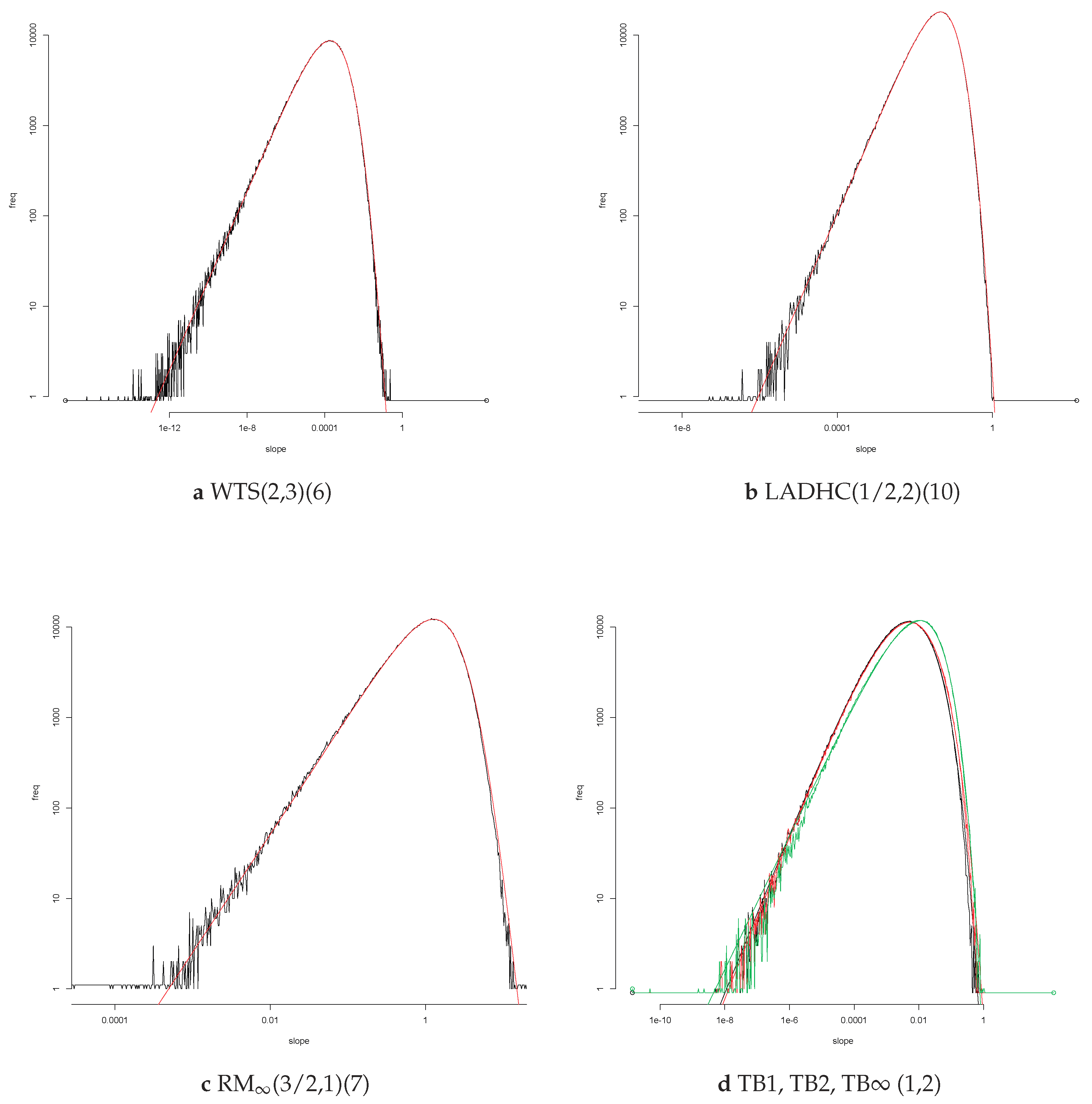
Of the four parameters of the EGBP distribution, there is one, the slope of the left asymptote of ψE, which we can link to the tail indices (ξ,η). It would be of interest to know how the remaining three parameters depend on the tail indices, the shape of the error density and the estimator. In the text below, we define the optimal fit. Let S denote the variable with density where y0 − ψ yields the optimal fit. We consider two issues:
- How close is the theoretical sd to the empirical sd listed in the tables in Section 7?
- How does the distance between the loglog frequency plot of and compare to the distance between the log of the frequency plot of S and .
Our loglog frequency plots fr and gr are random piecewise linear functions with twenty bins per unit. We round off to an integer value m the random value , count the number, n, of occurrences of m in the million simulations and connect the points . The random fluctuations in the resulting plot fr are clearly visible, in particular in the tails. We choose the base line at level −1/10 so as to see unique occurrences, n = 1. The global shape is a concave curve like a parabola but with asymptotes with finite slopes. Let be a logconcave density. Define the distance
where we take the expectation with respect to the probability measure with atoms of size n/106 in m/20. To see whether the fit is good we simulate a million samples from the density g, construct gr, the log of the corresponding frequency plot, and compute the distance d(gr,g). Actually, we simulate twenty batches of a million samples and write down the average and sd of the distances in the notation of Equation (6) introduced in Section 2.
What logconcave density should one choose to obtain a good fit? The density g(s) = c/cosh(s) is symmetric. The function has asymptotes with slope ±1. It satisfies and . A scale transformation in the vertical and the horizontal direction will transform φ0 into the function which satisfies and . The asymptotes of φ have slope ±c/a. We still need to modify the function to have asymptotes whose absolute slopes assume different values. This may be achieved by replacing 1/cosh(s) by one of the functions below:
Note that the scale transformation of φ in the vertical direction corresponds to a power transformation of the density. We now have a three-dimensional family of analytic convex functions φ which are determined by the absolute values of the asymptotic slopes and the curvature at the origin. We still need a horizontal translation to fit the densities to the frequency plot fr.
Let Φ denote this four-dimensional space of convex analytic functions φ. Each function φ ∈ Φ is determined by four parameters: in . The corresponding space of dfs is EGBP. For a given loglog frequency plot fr choose the density with φ0 ∈ Φ to minimize the distance . Let
denote this minimal distance. Let gr denote the log of the frequency plot for a sample of size n = 106 from g0 and set . It may happen that d0 > d. Perhaps one should compare d not to d0, the distance between gr and g0, but to , the minimum of over all densities , φ ∈ Φ. Do that for twenty batches of a million simulations from the density g0.
Example A4.
For the estimators HB40(3), HB0(3) and RM(9) applied to samples of size n = 100 of points (Xi, Yi) where the X1 > ⋯ > g100 have a Pareto(1) distribution, Xi = 1/Ui, for the order statistics Ui of a sample from the uniform distribution on (0,1) and errors Yi from a Cauchy distribution scaled by its IQD, we obtain (d, d0, d1) = (0.01965, 0.019[1], 0.019[1]), (0.02036, 0.020[1], 0.019[1]) and (0.02077, 0.020[1], 0.020[1]).
Here is a crude estimate of the distance between the log of the frequency plot gr for a million simulations from the density g and the density. Let b0 denote the number of non-empty bins. Then,
In our case, b0 ≈ 340, which gives d ≈ 0.017.
Indeed, the number Nk of sample points in the kth bin Bk is binomial(n,pk) where n = 106 is the number of simulations and pk is the integral of g over the bin Bk. Hence, where with qk = 1 − pk close to one and Uk asymptotically standard normal for npk → ∞. Hence, and
The condition that be large does not hold for the bins in the tails. The loglog frequency plots are based on a million values of . Most of these occur in the centre. The tails, say the part where the frequency, the number of entries Nk in a bin, is less than a hundred is less than 0.5% of the total. It is this part which determines the tail behaviour. The distance between the smooth EGBP-fit y0 − ψ and the loglog frequency plot fr is determined by the middle part. A good fit in the tails is a bonus.
Appendix C.7. Variations in the Error Density at the Origin
What happens if one replaces the Student density by a symmetric density which is constant on a neigbourhood of the origin, or which has a vertex at the origin, or a zero, or a pole? We introduce three error variables with symmetric densities and with tail index η = 1. Start with variables Zs, Zu, and Zp with IQD = 2. These variables have symmetric densities and satisfy . The variable Zs has a Student distribution. It is the Cauchy variable with density . The variable zu has a density which is constant with value 1/4 on the interval (− 1, 1) and has Pareto tails: , z > 1. The variable zp is the symmetric version of a shifted Pareto variable , z > 0.
Define the corresponding error variables Yt = Zt/2 for t = s, u, p. The explanatory variables are Xi = 1/Ui where U1, …, Un are the increasing order statistics from the uniform distribution on (0,1). We use the estimators HB0[3] and HB40[3] to determine the empirical sd and to construct loglog frequency plots fr. One may expect HB40 to be less sensitive to the precise form of the density at the origin since it is based on the behaviour of the df at the 0.4 and 0.6 quantiles of the error distribution. Determine the EGBP approximation in these six cases, and the theoretical sd, the square root of . We also compute the distance . We then construct twenty plots gr corresponding to twenty batches of a million simulations from g0, and compute the distances and where is the best EGBP-approximation to gr.
If U is uniformly distributed on the interval (0,1), then U2 has density and has density 2u2 on (0,1). In general, for r > 0. For the three variables Zt introduced above, define samples of by replacing Zt by sign(Zt)|Zt|r when Zt lies in the interval (−1,1). The density of is asymptotic to ct|y| at the origin if r = 1/2 and asymptotic to if r = 2. We also check how good the EGBP-fit is for errors with these densities in Table A3, Table A4, Table A5, Table A6, Table A7 and Table A8 below.
The final plot below, Figure A5, shows the EGBP-fit to the loglog frequency plot for . The error has a Cauchy distribution scaled by its IQD, the explanatory variables are Pareto with tail index ξ = 1. The figure shows two things: LS is not a good estimator for (ξ,η) = (1,1). The right tail of the loglog frequency plot extends beyond 10,000. The EGBP fit is good.
Figure A5.
EGBP approximations for (ξ,η) = (1,1) to three loglog frequency plots for and one for . The error densities , in (b,c) are asymptotic to at the origin. In the first and fourth plots, the error is Cauchy scaled by its IQD.
Figure A5.
EGBP approximations for (ξ,η) = (1,1) to three loglog frequency plots for and one for . The error densities , in (b,c) are asymptotic to at the origin. In the first and fourth plots, the error is Cauchy scaled by its IQD.
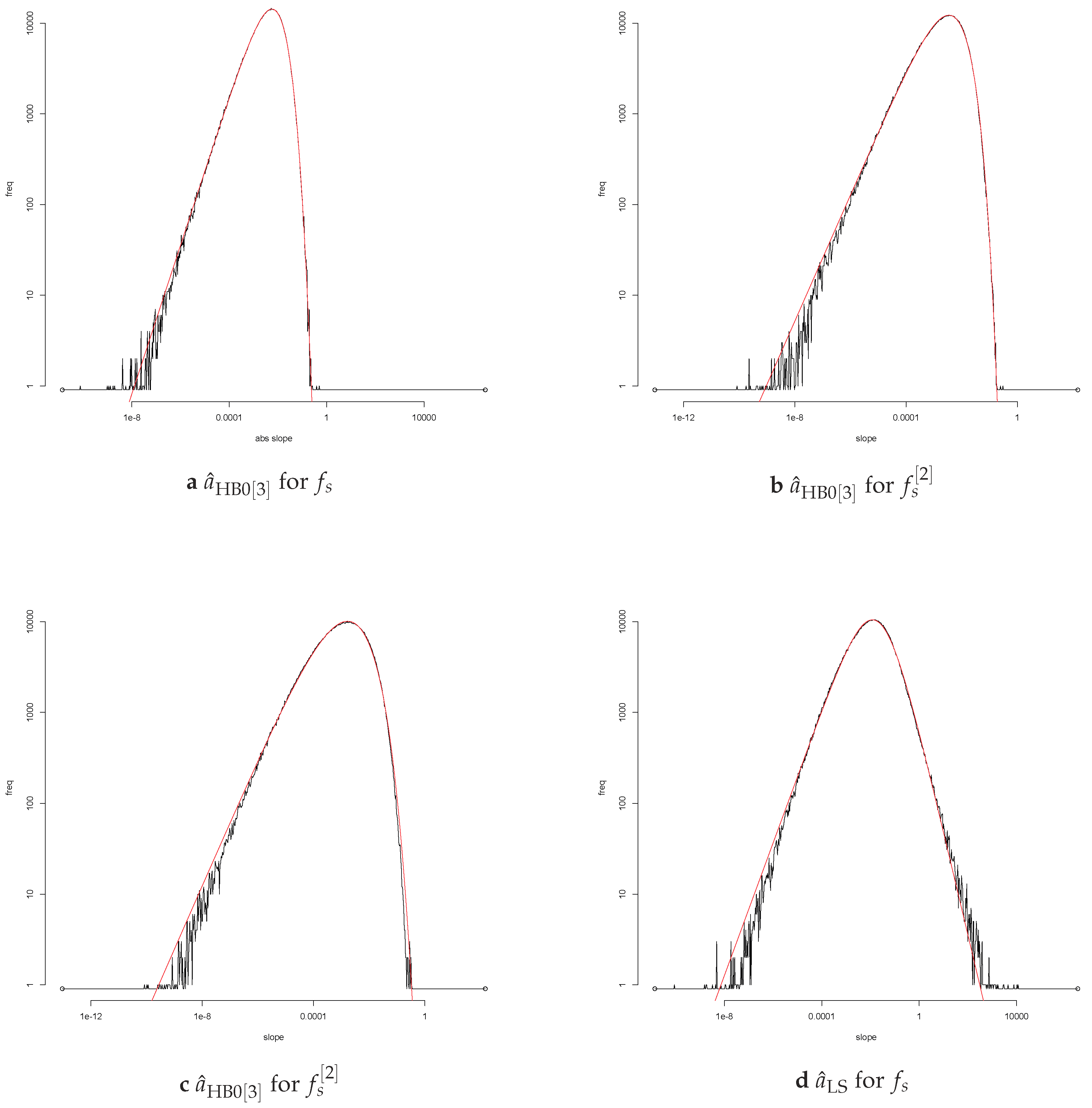
Table A3.
.
| Density | emp sd | theor sd | |||
|---|---|---|---|---|---|
| 0.01158[5] | 0.01158 | 0.01965 | 0.019[1] | 0.019[1] | |
| 0.01105[5] | 0.01106 | 0.01790 | 0.019[1] | 0.019[1] | |
| 0.0122[2] | 0.01223 | 0.02012 | 0.0200[5] | 0.0192[5] |
Table A4.
.
| Density | emp sd | theor sd | |||
|---|---|---|---|---|---|
| 0.01201[5] | 0.01200 | 0.02036 | 0.020[1] | 0.019[1] | |
| 0.01205[5] | 0.01218 | 0.01893 | 0.0192[5] | 0.0188[5] | |
| 0.0120[1] | 0.01217 | 0.02050 | 0.0193[5] | 0.0189[5] |
Table A5.
.
| Density | emp sd | theor sd | |||
|---|---|---|---|---|---|
| 0.00952[5] | 0.009545 | 0.02022 | 0.0194[5] | 0.0193[5] | |
| 0.00963[5] | 0.009643 | 0.02100 | 0.019[1] | 0.019[1] | |
| 0.0096[2] | 0.009824 | 0.02295 | 0.0203[5] | 0.0201[5] |
Table A6.
.
| Density | emp sd | theor sd | |||
|---|---|---|---|---|---|
| 0.00847[5] | 0.008634 | 0.03120 | 0.0209[5] | 0.0208[5] | |
| 0.00881[5] | 0.008888 | 0.03094 | 0.0200[5] | 0.0199[5] | |
| 0.0083[1] | 0.008916 | 0.03863 | 0.0210[5] | 0.0209[5] |
Table A7.
.
| Density | emp sd | theor sd | |||
|---|---|---|---|---|---|
| 0.01209[5] | 0.01226 | 0.01971 | 0.0194[5] | 0.0190[5] | |
| 0.01103[5] | 0.01115 | 0.01892 | 0.0193[5] | 0.0190[5] | |
| 0.0134[2] | 0.01338 | 0.02144 | 0.020[1] | 0.019[1] |
Table A8.
.
| Density | emp sd | theor sd | |||
|---|---|---|---|---|---|
| 0.01518[5] | 0.01525 | 0.01727 | 0.019[1] | 0.019[1] | |
| 0.0148[1] | 0.01482 | 0.01876 | 0.018[1] | 0.018[1] | |
| 0.0157[2] | 0.01585 | 0.02003 | 0.0191[5] | 0.0186[5] |
It is the distribution of the estimator which determines how good it is, in particular the right tail of the distribution of . This right tail determines the risk. The loglog frequency plot gives a good description of the tail behaviour. A steep decrease on the right, indicates a light right tail for . A good EGBP fit means that the logconcave density of the EGBP variable S agrees well with the distribution of the variable . Moreover, the theoretical sd being close to the empirical sd of indicates that the good fit extends to the right tail. The simulations in this paper suggest that for Student errors the loglog frequency plots for the absolute value of the estimator may often be fitted accurately by the exponent of the logconcave EGBP densities, and that this good fit extends to the right tail. The results above show that the good fit also holds for symmetric densities with a zero or a singularity at the origin.
References
- Balkema, Guus. Least Absolute Deviation and Balance. Unpublished work.
- Balkema, Guus, and Paul Embrechts. 2007. High Risk Scenarios and Extremes. A Geometric Approach. Zurich Lectures in Advanced Mathematics. Zurich: European Mathematical Society. [Google Scholar]
- Bassett, Gilbert, Jr., and Roger Koenker. 1978. Asymptotic theory of Least Absolute Error regression. Journal of the American Statistical Association 73: 618–22. [Google Scholar] [CrossRef]
- Dielman, Terry E. 2005. Least absolute value regression: Recent contributions. Journal of Statistical Computation and Simulation 75: 263–86. [Google Scholar] [CrossRef]
- Drygas, Hilmar. 1976. Weak and strong consistency of least squares estimates in regression models. Zeitschrift für Wahrscheinlichkeitstheorie und Verwandte Gebiete 34: 119–27. [Google Scholar] [CrossRef]
- De Haan, Laurens, and Ana Ferreira. 2006. Extreme Value Theory: An Introduction. Berlin: Springer. [Google Scholar]
- Eddington, Arthur Stanley. 1914. Stellar Movements and the Structure of the Universe. London: Macmillan. [Google Scholar]
- Fischler, Martin A., and Robert C. Bolles. 1981. Random sample consensus: A paradigm for model fitting with applications to image analysis and automated cartography. Communications of the ACM 24: 381–95. [Google Scholar] [CrossRef]
- Heffernan, Janet E., and Jonathan A. Tawn. 2004. A conditional approach for multivariate extreme values. Journal of the Royal Statistical Society 66: 497–546. [Google Scholar] [CrossRef]
- Heffernan, Janet E., and Sidney I. Resnick. 2007. Limit laws for random vectors with an extreme component. The Annals of Applied Probability 17: 537–71. [Google Scholar] [CrossRef]
- Jaeckel, Louis A. 1972. Estimating regression coefficients by minimizing the dispersion of the residuals. The Annals of Mathematical Statistics 43: 1449–58. [Google Scholar] [CrossRef]
- Koenker, Roger. 2000. Galton, Edgeworth, Frisch, and the prospects for quantile regression in econometrics. Journal of Econometrics 95: 347–74. [Google Scholar] [CrossRef]
- Kuan, Chung-Ming. 2007. Asymptotic Least Squares Theory: Part I. Available online: http://homepage.ntu.edu.tw/c̃kuan/pdf/et01/et_Ch6.pdf (accessed on 22 August 2018).
- Lehmann, Erich L. 1983. Theory of Point Estimation. New York: Wiley. [Google Scholar]
- Mikosch, Thomas, and Casper G. de Vries. 2013. Heavy tails of OLS. Journal of Econometrics 172: 205–21. [Google Scholar] [CrossRef]
- Nagya, Gábor. 2018. Sector based linear regression, a new robust method for the multiple linear regression. Acta Cybernetica 23: 1017–38. [Google Scholar] [CrossRef]
- Nolan, John P., and Diana Ojeda-Revah. 2013. Linear and non-linear regression with stable errors. Journal of Econometrics 172: 186–94. [Google Scholar] [CrossRef]
- Postnikov, Eugene B., and Igor M. Sokolov. 2015. Robust linear regression with broad distributions of errors. Physica A 434: 257–67. [Google Scholar] [CrossRef]
- Rousseeuw, Peter J. 1984. Least median of squares regression. Journal of the American Statistical Association 79: 871–80. [Google Scholar] [CrossRef]
- Rousseeuw, Peter J. 1991. Tutorial to robust statistics. Journal of Chemometrics 5: 1–20. [Google Scholar] [CrossRef]
- Ruppert, David, and Raymond J. Carroll. 1980. Trimmed least squares estimation in the linear model. Journal of the American Statistical Association 75: 828–38. [Google Scholar] [CrossRef]
- Samorodnitsky, Gennady, Svetlozar T. Rachev, Jeong-Ryeol Kurz-Kim, and Stoyan V. Stoyanov. 2007. Asymptotic distribution of unbiased linear estimators in the presence of heavy-tailed stochastic regressors and residuals. Probability and Mathematical Statistics 27: 275–302. [Google Scholar]
- Sen, Pranab Kumar. 1968. Estimates of the regression coefficient based on Kendall’s tau. Journal of the American Statistical Association 63: 1379–89. [Google Scholar] [CrossRef]
- Siegel, Andrew F. 1982. Robust regression using repeated medians. Biometrika 69: 242–44. [Google Scholar] [CrossRef]
- Sievers, Gerald L. 1978. Weighted rank statistics for simple linear regression. Journal of the American Statistical Association 73: 628–31. [Google Scholar] [CrossRef]
- Smith, V. Kerry. 1973. Least squares regression with Cauchy errors. Oxford Bulletin of Economics and Statistics 35: 223–31. [Google Scholar] [CrossRef]
- Theil, Henri. 1950. A rank-invariant method of linear and polynomial regression analysis. Proceedings of the KNAW 53: 386–92, 521–25, 1397–412. [Google Scholar]
- Van de Geer, Sara Anna. 1988. Asymptotic normality of minimum L1-norm estimators in linear regression. In Report. MS-R8806. Amsterdam: CWI. [Google Scholar]
| 1. | Probabilities for the explanatory variables may be reduced to probabilities for order statistics from the uniform distribution on . Here, we use that, given , the quotient is uniformly distributed on and that . |
| 2. | I thank Michael Feast from the Department of Astronomy of the University of Cape Town for drawing my attention to these words. |
Figure 1.
On the grid (ξ, η) ∈ {0, 1/2, 1, 3/2, 2, 3} × {0, 1/3, 1/2, 2/3, 1, 3/2, 2, 3, 4}, the optimal estimators for Student errors are: LS, a red circle, and TS, a pink disk; LAD, a light blue △, TB1, a blue ▽, LADPC, a dark green filled ▽, and LADHC a light green filled △; and HB0 a purple □, and HB40, an orange ⊠. On the right is a sample for (ξ,η) = (3,1) with Student errors. The true regression line is the horizontal axis. The LAD (Least Absolute Deviation) estimate drawn in the plot is obviously a bad estimate. This line is also the RMP (RightMost Point) estimate.

Figure 2.
Frequencies of the absolute slope for (ξ,η) = (3,4). On the left: The LAD estimator yields an empirical sd = 0e+16[1]. On the right: The Right Median estimator based on the 21 rightmost sample points, RM(21), yields an empirical sd = 0.00027[5]. The Hill estimate of the right tail index of the distribution of is 3.87; for it is 0.436.
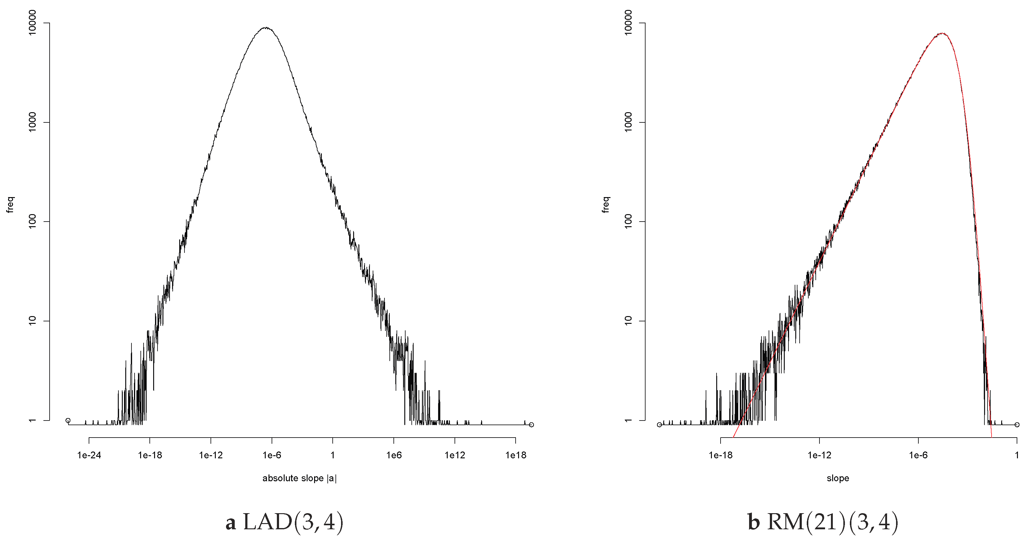
Figure 3.
The sd (on two scales) of the slopes An and (dashed) of the LS estimates of the regression line y = ax + b and the regression ray y = ax for the n = 20,50,100,200,500,1000 (grey, azure, black, red, green, and blue) and ∞ (purple) rightmost points of the Poisson point process N0 for standard normal errors.

Figure 4.
Log frequency of for ξ = η = i/10 for i = 2, …, 7, and 0.999 quantiles of . The Hill estimates of the tail index of are based on the 500 largest absolute observations.
Figure 4.
Log frequency of for ξ = η = i/10 for i = 2, …, 7, and 0.999 quantiles of . The Hill estimates of the tail index of are based on the 500 largest absolute observations.

Figure 5.
Log frequencies for the estimates (full line) and (dashed) of the slope of the regression line based on a million simulations of a sample of 100 points , with X standard exponential and Y* of the form O × U2 (red), O × U (black), (green) and O × (1 + U)/2 (blue) where U is standard uniform on (0, 1) and O is a fair sign independent of U. Note that depends on the density of Y* at the median; on the density at the 0.4 and 0.6 quantiles.

Figure 6.
Loglog frequencies of |aLAD| for ξ = 1/4, η = 1,4. The concave red curve is the EGBP fit. On the left: The empirical sd is 0.243[2], the theoretical sd of the EGBP fit is 0.2425. On the right: 2e + 6[5e + 6] and ∞. On the left: the Hill estimate of the tail index based on the 1001 rightmost points is 0.18 yielding a finite fifth moment. On the right: 0.89 yields an infinite second moment.
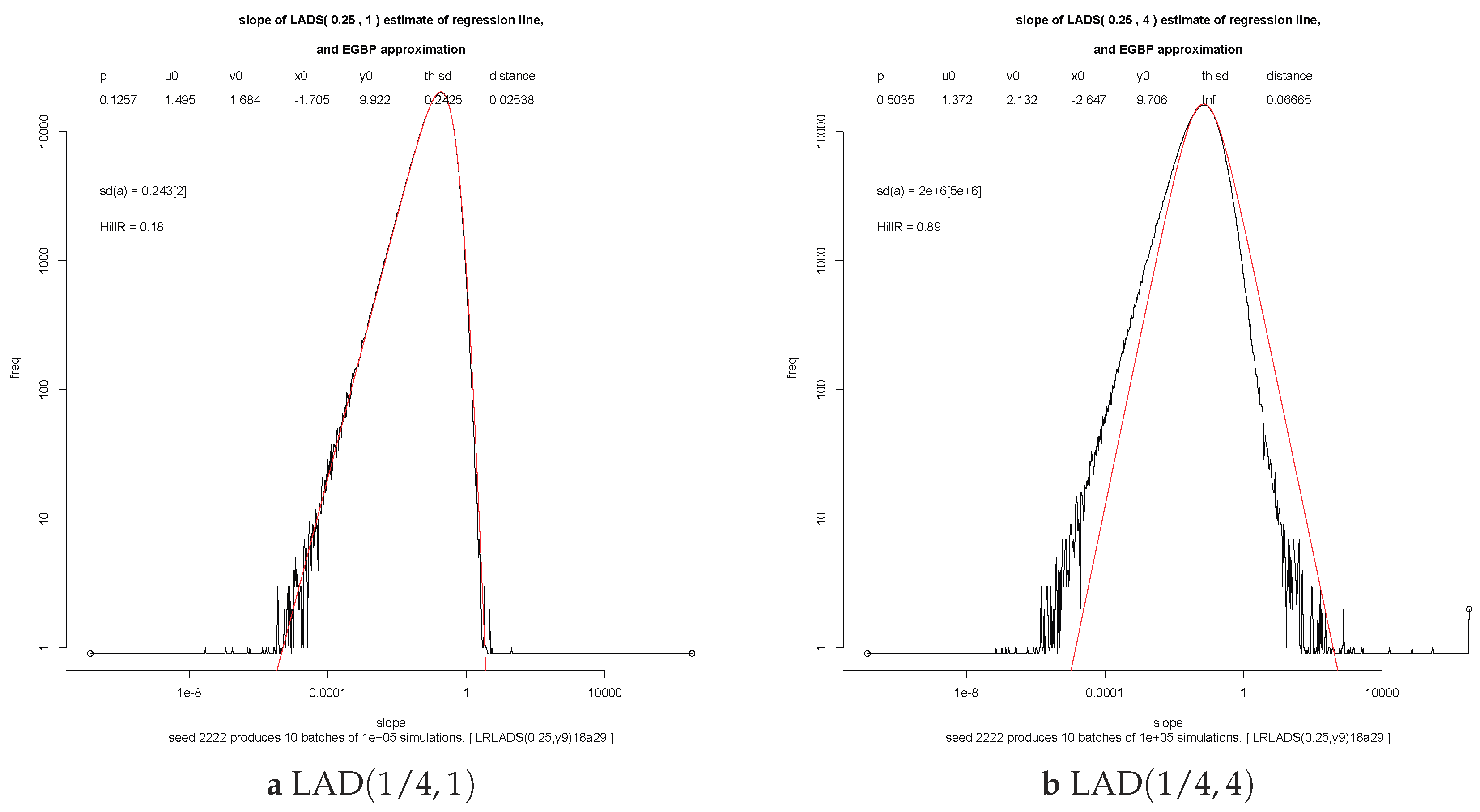
Figure 7.
On the left: , for ten batches of 105 simulations of a sample of 100 Student variables scaled by their IQD and trimmed by m on both sides, is minimal for m = 1, 23, 29, 34, 39, 44, 46, 48, 49 for tail index η = 0, 1/3, 1/2, 2/3, 1, 3/2, 2, 3, 4 (black, red, green, blue, brown, purple, orange, azure, and grey). On the right: A bimodal loglog frequency plot for for (ξ,η) = (3,3), (m, p) = (22, 1) and Pareto errors. The red (green) curve describes the 629,341 negative (370,659 positive) outcomes. The black curve describes the sum, the one million outcomes of the absolute value. Here, for the state function with p = 1 and 0.0137[1] without reward (p = 0). The minimal value is 0.00016[5] for p = 15. An extra parameter yields for (m, p, r) = (25, 30, 0.6).
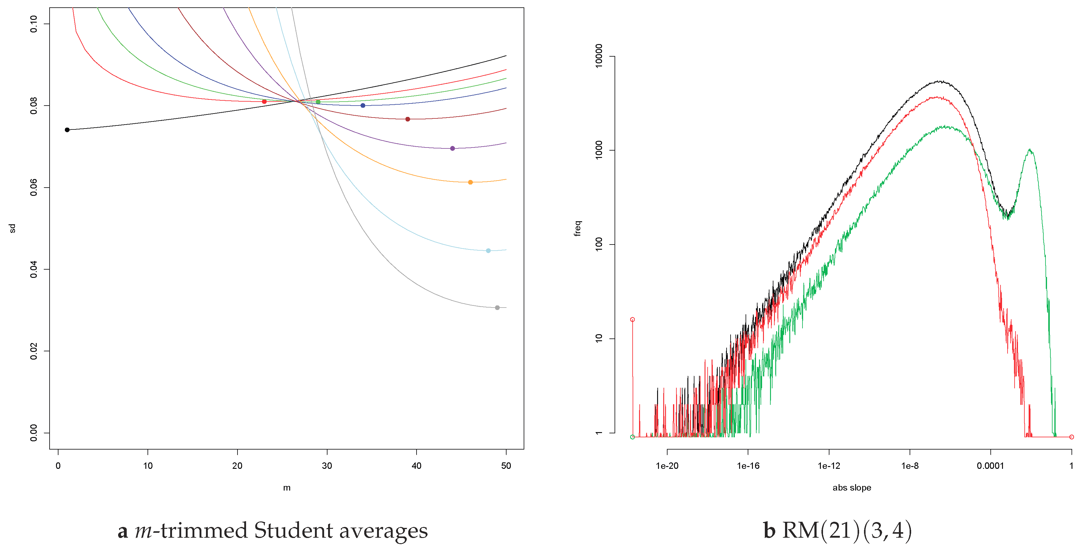
Figure 8.
The average square root of the average loss for for Student (left, m = 30) and Pareto (right, m = 29) errors for (ξ,η) = (3,3) and ten batches of 105 simulations. The curves describe the behaviour of as a function of p for different values of r = 0.15, 0.2, 0.25, 0.3, 0.4, 0.5 (Student) and r = 3:8/10 (Pareto) with colours black, red, green, blue, brown, and purple. The erratic behaviour on the right is symptomatic for Pareto errors.

Figure 9.
The square root of the average loss for WLTS(16, p, r) at (ξ,η) = (1,1) for Student errors (full lines) and Pareto errors (dashed) scaled by the IQD for p ranging from 0.1 to 200 and r = 0.01 (grey), 0.02 (pink), 0.05 (dark green), 0.1 (black), 0.2 (red), 0.3 (green), 0.4 (blue), 0.5 (brown), 0.6 (purple), 1 (orange), and 2 (azure). The optimal values of (p, r) are (0.2, 0.4) (Student) and (200, 0.5) (Pareto).

Table 1.
The empirical sd for .
| 0 | 1/2 | 1 | 3/2 | 2 | 3 | 4 | |
|---|---|---|---|---|---|---|---|
| 0 | 0.0969[2] | 0.0951[2] | 0.0917[5] | 0.0869[2] | 0.0810[5] | 0.0681[5] | 0.0560[5] |
| 1/2 | 0.0641[2] | 0.0690[2] | 0.1[1] | 3[5] | 40[50] | 1e+7[1] | 2e+10[5] |
Table 2.
Quantiles , empirical sd and slope.
| 1/5 | 3/10 | 2/5 | 1/2 | 3/5 | 7/10 | |
|---|---|---|---|---|---|---|
| 0.999 quantile | 1.28 | 0.999 | 1.09 | 1.33 | 1.95 | 2.87 |
| emp sd | 0.312[1] | 0.196[1] | 0.16[1] | 0.19[5] | 0.3[1] | 1[1] |
| Hill est | 0.15[1] | 0.23[1] | 0.35[2] | 0.46[2] | 0.59[5] | 0.69[5] |
Table 3.
Three estimators.
| LS | 0.0467[1] | 0.0603[2] | 0.0739[2] | 0.0798[2] |
| LAD | 0.0308[1] | 0.0982[2] | 0.1774[5] | 0.2132[5] |
| LAD40 | 0.0376[1] | 0.0879[2] | 0.1069[2] | 0.0677[5]. |
Table 4.
The empirical sd of the estimate of the slope for LS, LAD and RMP. The breakdown of LS for is dramatic. Even the simple RMP performs better. For , Least Absolute Deviation is optimal.The sds decrease as ξ increases, as is to be expected, and the relative size of the fluctuations increases too.
| 1/2 | 1 | 3/2 | 2 | 5/2 | 3 | ||
|---|---|---|---|---|---|---|---|
| 0.0774[2] | 0.0518[1] | 0.00702[2] | 0.00122[1] | 0.000245[5] | 0.000054[2] | 0.0000131[5] | |
| 1/3 | 0.118[1] | 0.0790[5] | 0.0107[1] | 0.00186[2] | 0.00037[1] | 0.000081[5] | 0.000019[1] |
| 1/2 | 0.23[1] | 0.15[1] | 0.020[1] | 0.0034[2] | 0.0007[1] | 0.00015[5] | 0.00004[1] |
| 2/3 | 0[100] | 30[50] | 0[10] | 1[1] | 0.1[2] | 0.01[2] | 0.001[2] |
| 1 | 0[100000] | 20000[50000] | 3000[5000] | 0[1000] | 0[100] | 2[5] | 0.1[1] |
| 0.0971[2] | 0.0641[2] | 0.00859[2] | 0.00149[1] | 0.000295[5] | 0.000066[2] | 0.0000157[5] | |
| 1/3 | 0.0959[2] | 0.0670[1] | 0.00946[2] | 0.00169[1] | 0.000344[5] | 0.0000764[5] | 0.0000184[5] |
| 1/2 | 0.0952[2] | 0.0690[5] | 0.0103[2] | 0.00190[5] | 0.00039[2] | 0.000087[5] | 0.000021[2] |
| 2/3 | 0.0941[2] | 0.072[1] | 0.0120[2] | 0.003[1] | 0.00062[5] | 0.00014[5] | 0.00004[1] |
| 1 | 0.0918[5] | 0.11[5] | 1[1] | 0.0[1] | 0.008[5] | 0.00[1] | 0.001[1] |
| 0.1966[5] | 0.0974[5] | 0.0116[1] | 0.00189[5] | 0.00036[1] | 0.000078[5] | 0.000018[1] | |
| 1/3 | 0.290[5] | 0.144[2] | 0.0171[5] | 0.0028[1] | 0.00052[2] | 0.000111[5] | 0.000026[2] |
| 1/2 | 0.6[1] | 0.3[1] | 0.04[1] | 0.006[2] | 0.0011[5] | 0.0002[1] | 0.00005[5] |
| 2/3 | 4[5] | 2[2] | 0.3[5] | 0.04[5] | 0.01[1] | 0.002[2] | 0.0003[5] |
| 1 | 300[500] | 200[200] | 20[50] | 3[5] | 1[1] | 0.1[2] | 0.02[5] |
Table 5.
Theempirical sd of for Student errors with tail index .
| 0 | 1/3 | 1/2 | 2/3 | 1 | 3/2 | 2 | 3 | 4 | |
|---|---|---|---|---|---|---|---|---|---|
| 0 | 0.0969[2] | 0.0959[2] | 0.0951[2] | 0.0941[2] | 0.0917[2] | 0.0869[2] | 0.0810[5] | 0.0681[5] | 0.0560[5] |
| 1/4 | 0.2328[5] | 0.2363[5] | 0.238[1] | 0.2389[5] | 0.243[2] | 0.26[2] | 0.4[2] | 10000[10000] | 2e+6[5] |
| 1/2 | 0.0641[2] | 0.0670[2] | 0.0690[2] | 0.072[1] | 0.1[1] | 3[5] | 40[50] | 1e+7[2] | 2e+10[5] |
| 1 | 0.00861[5] | 0.00943[5] | 0.0104[5] | 0.012[1] | 1[1] | 20[20] | 10000[10000] | 2e+6[2] | 0e+15[2] |
Table 6.
Empirical sd of the slope for estimators without a parameter for Student errors.
| 0 | 0.2578[5] | 0.2371[5] | 0.2227[5] | ||||
| 1/3 | 0.2094[5] | ||||||
| 1/2 | 0.26[5] | ||||||
| 2/3 | 1.6[5] | ||||||
| 1 | 200[100] | ||||||
| 3/2 | 1e+6[2e+6] | ||||||
| 2 | 3e+9[5e+9] | ||||||
| 3 | 0[1e+17] | 0.1242[5] | 0.153[1] | ||||
| 4 | 2e+24[5e+24] | 0.1159[5] | 0.124[5] | 0.192[5] | |||
| LS | LAD | LADPC | TS | TB1 | TB2 | TB∞ | |
| 0 | 0.258[1] | 0.230[1] | 0.2159[5] | ||||
| 1/3 | 0.2044[5] | 0.1829[5] | 0.1824[5] | ||||
| 1/2 | 0.17[2] | 0.1827[5] | 0.1640[5] | 0.170[1] | |||
| 2/3 | 1.0[5] | 0.163[1] | 0.148[1] | 0.1604[5] | |||
| 1 | 120[50] | ||||||
| 3/2 | 0[1e+6] | 3[5] | |||||
| 2 | 1e+9[1e+9] | 40[50] | |||||
| 3 | 1e+16[1e+16] | 1e+7[2e+7] | 0.1298[5] | 0.153[2] | |||
| 4 | 2e+23[5e+23] | 2e+10[5e+10] | 0.1257[5] | 0.160[5] | 0.21[1] | ||
| LS | LAD | LADPC | TS | TB1 | TB2 | TB∞ | |
| 0 | 0.01660[5] | 0.0647[2] | 0.0558[2] | 0.0514[2] | |||
| 1/3 | 0.0491[2] | 0.0424[2] | 0.0424[2] | ||||
| 1/2 | 0.0432[2] | 0.0376[2] | 0.0393[1] | ||||
| 2/3 | 0.1[1] | 0.0382[2] | 0.0336[2] | 0.0369[2] | |||
| 1 | 10[10] | 1[1] | 0.0305[5] | 0.0279[5] | 0.0333[1] | ||
| 3/2 | 30000[20000] | 20[20] | 0.0312[5] | ||||
| 2 | 1e+8[2e+8] | 10000[10000] | 0.0286[1] | 0.0316[5] | |||
| 3 | 0[1e+16] | 2e+6[2e+6] | 0.0314[2] | 0.032[1] | 0.038[1] | ||
| 4 | 2e+23[5e+23] | 0[2e+15] | 0.0320[1] | 0.049[1] | 0.055[1] | ||
| LS | LAD | LADPC | TS | TB1 | TB2 | TB∞ | |
| 0 | 0.00260[2] | 0.00432[2] | 0.0220[2] | 0.0183[1] | 0.0164[1] | ||
| 1/3 | 0.00491[2] | 0.0160[1] | 0.0133[1] | 0.0131[1] | |||
| 1/2 | 0.00521[2] | 0.0137[1] | 0.0116[1] | 0.0120[1] | |||
| 2/3 | 0.02[2] | 0.0120[1] | 0.0103[1] | 0.0112[1] | |||
| 1 | 3[5] | 0.1[1] | 0.00626[5] | 0.0093[2] | 0.0085[1] | 0.0101[1] | |
| 3/2 | 5000[5000] | 10[10] | 0.00730[5] | 0.0072[1] | 0.0074[1] | 0.0095[1] | |
| 2 | 2e+7[5e+7] | 1e+6[2e+6] | 0.00830[5] | 0.0078[1] | 0.0099[2] | ||
| 3 | 1e+15[2e+15] | 1e+8[2e+8] | 0.00968[5] | 0.0117[5] | 0.0129[5] | ||
| 4 | 0[1e+23] | 3e+12[5e+12] | 0.0104[1] | 0.0074[2] | 0.0187[5] | 0.020[1] | |
| LS | LAD | LADPC | TS | TB1 | TB2 | TB∞ | |
| 0 | 0.000645[5] | 0.00126[1] | 0.0086[1] | 0.00685[5] | 0.00597[5] | ||
| 1/3 | 0.00145[1] | 0.00596[5] | 0.00482[5] | 0.00463[5] | |||
| 1/2 | 0.00154[1] | 0.00502[5] | 0.00415[5] | 0.00422[5] | |||
| 2/3 | 0.004[5] | 0.00165[1] | 0.00431[5] | 0.00363[5] | 0.00388[5] | ||
| 1 | 1[1] | 0.01[2] | 0.00189[2] | 0.0033[1] | 0.00295[5] | 0.00348[5] | |
| 3/2 | 1000[1000] | 1[1] | 0.00227[1] | 0.00254[5] | 0.00266[5] | 0.00334[5] | |
| 2 | 0[1e+7] | 0[100000] | 0.00266[5] | 0.00229[5] | 0.00292[5] | 0.0036[1] | |
| 3 | 1e+14[5e+14] | 0[1e+7] | 0.00328[2] | 0.0025[1] | 0.0047[2] | 0.0050[2] | |
| 4 | 1e+22[2e+22] | 1e+15[2e+15] | 0.00372[5] | 0.0032[2] | 0.0079[2] | 0.0081[5] | |
| LS | LAD | LADPC | TS | TB1 | TB2 | TB∞ | |
| 0 | 0.000049[1] | 0.000133[2] | 0.00161[5] | 0.00122[2] | 0.00099[2] | ||
| 1/3 | 0.000053[1] | 0.000155[2] | 0.00103[2] | 0.00079[2] | 0.00071[2] | ||
| 1/2 | 0.000054[1] | 0.000166[2] | 0.00084[2] | 0.00065[1] | 0.00063[2] | ||
| 2/3 | 0.0002[2] | 0.000179[5] | 0.00070[1] | 0.00057[1] | 0.00058[2] | ||
| 1 | 0.02[5] | 0.001[1] | 0.000209[5] | 0.00051[2] | 0.00045[1] | 0.00051[2] | |
| 3/2 | 30[50] | 0.1[1] | 0.000261[5] | 0.00040[1] | 0.00042[1] | 0.00051[1] | |
| 2 | 100000[200000] | 0[1000] | 0.00032[1] | 0.00038[2] | 0.00051[5] | 0.00057[5] | |
| 3 | 0[1e+13] | 300000[500000] | 0.00044[1] | 0.00049[5] | 0.0009[1] | 0.0009[1] | |
| 4 | 1e+20[5e+20] | 1e+13[2e+13] | 0.00055[2] | 0.0007[1] | 0.0016[1] | 0.0016[5] |
Table 7.
Empirical sd of the slope for estimators with a parameter for Student errors.
| 0 | 0.0706[2] | |||||
| 1/3 | 0.0722[2] | |||||
| 1/2 | 0.0726[2] | |||||
| 2/3 | 0.0727[2] | |||||
| 1 | 0.0717[1] | |||||
| 3/2 | 0.0680[2] | |||||
| 2 | 0.0626[2] | |||||
| 3 | 0.0475[2] | |||||
| 4 | 0.129[1] | 0.0331[2] | ||||
| RM[r] | HB40[d] | HB0[d] | LADHC[d] | WTS[p] | ||
| 0 | 0.0398[1] | |||||
| 1/3 | 0.0421[1] | |||||
| 1/2 | 0.0428[1] | |||||
| 2/3 | 0.0430[1] | |||||
| 1 | 0.0424[1] | |||||
| 3/2 | 0.0396[1] | |||||
| 2 | 0.0356[1] | |||||
| 3 | 0.0264[1] | |||||
| 4 | 0.129[1] | 0.01825[5] | ||||
| RM[r] | HB40[d] | HB0[d] | LADHC[d] | WTS[p] | ||
| 0 | 0.00706[5] | |||||
| 1/3 | 0.00860[5] | |||||
| 1/2 | 0.00936[5] | |||||
| 2/3 | 0.0100[1] | |||||
| 1 | 0.0109[1] | |||||
| 3/2 | 0.0110[1] | |||||
| 2 | 0.01040[5] | |||||
| 3 | 0.00839[5] | |||||
| 4 | 0.0288[5] | 0.00617[5] | ||||
| RM[r] | HB40[d] | HB0[d] | LADHC[d] | WTS[p] | ||
| 0 | 0.00123[1] | |||||
| 1/3 | 0.00159[2] | |||||
| 1/2 | 0.00183[2] | |||||
| 2/3 | 0.00204[2] | |||||
| 1 | 0.00236[2] | |||||
| 3/2 | 0.00261[5] | |||||
| 2 | 0.00269[5] | |||||
| 3 | 0.00243[5] | |||||
| 4 | 0.0082[5] | 0.00200[5] | ||||
| RM[r] | HB40[d] | HB0[d] | LADHC[d] | WTS[p] | ||
| 0 | 0.000245[5] | |||||
| 1/3 | 0.00033[1] | |||||
| 1/2 | 0.00038[1] | |||||
| 2/3 | 0.00044[1] | |||||
| 1 | 0.00054[2] | |||||
| 3/2 | 0.00065[2] | |||||
| 2 | 0.00070[2] | |||||
| 3 | 0.00072[2] | |||||
| 4 | 0.0025[1] | 0.00066[1] | ||||
| RM[r] | HB40[d] | HB0[d] | LADHC[d] | WTS[p] | ||
| 0 | 0.0000130[5] | |||||
| 1/3 | 0.000018[1] | |||||
| 1/2 | 0.000021[2] | |||||
| 2/3 | 0.000025[1] | |||||
| 1 | 0.000033[2] | |||||
| 3/2 | 0.000046[5] | |||||
| 2 | 0.000053[5] | |||||
| 3 | 0.000069[5] | |||||
| 4 | 0.000073[5] |
Table 8.
Empirical sd and bias of the slope for estimators with a parameter for Pareto errors.
| 0 | 0.0778[2] | |||||
| 0.0096[5] | 0.0086[5] | 0.0079[5] | 0.0088[2] | 0.0089[2] | −0.0280[5] | |
| 1/3 | 0.0823[2] | |||||
| 0.0122[5] | 0.0096[5] | 0.0100[5] | 0.0112[2] | 0.0099[2] | −0.0462[5] | |
| 1/2 | 0.0823[2] | |||||
| 0.0134[5] | 0.0097[5] | 0.0109[5] | 0.0118[2] | 0.0093[2] | −0.0561[2] | |
| 2/3 | 0.0812[2] | |||||
| 0.0129[5] | 0.0104[5] | 0.0110[2] | 0.0120[1] | 0.0088[2] | −0.0650[2] | |
| 1 | 0.1085[5] | 0.0702[5] | ||||
| 0.0145[5] | 0.0104[2] | 0.0118[2] | 0.0124[2] | 0.0068[2] | −0.0890[2] | |
| 3/2 | 0.1006[5] | 0.072[5] | ||||
| 0.0137[2] | 0.0096[2] | 0.0125[2] | 0.0133[1] | 0.0055[1] | −0.0762[2] | |
| 2 | 0.0917[5] | 0.0715[5] | 0.0708[5] | 0.055[1] | ||
| 0.0128[2] | 0.0087[2] | 0.0123[2] | 0.0126[2] | 0.0039[1] | −0.0657[1] | |
| 3 | 0.0733[5] | 0.0434[2] | 0.0556[5] | 0.0553[2] | 0.0376[5] | |
| 0.0108[2] | 0.0062[1] | 0.0110[2] | 0.0103[2] | 0.00149[5] | −0.0417[1] | |
| 4 | 0.0571[5] | 0.0296[2] | 0.0412[5] | 0.0408[2] | 0.0236[2] | |
| 0.0071[2] | 0.0040[1] | 0.0082[1] | 0.0078[2] | 0.00054[2] | −0.02674[5] | |
| RM[r] | HB40[d] | HB0[d] | LADHC[d] | WTS[p] | ||
| 0 | 0.0517[2] | |||||
| 0.0134[5] | 0.0101[2] | 0.0105[2] | 0.0098[2] | 0.0077[2] | −0.0131[2] | |
| 1/3 | 0.0534[2] | |||||
| 0.0165[5] | 0.0117[2] | 0.0129[2] | 0.0128[2] | 0.0099[2] | −0.0218[2] | |
| 1/2 | 0.0533[2] | |||||
| 0.0172[5] | 0.0124[2] | 0.0143[2] | 0.0140[2] | 0.0108[2] | −0.0263[1] | |
| 2/3 | 0.0535[5] | |||||
| 0.0179[5] | 0.0134[2] | 0.0149[2] | 0.0154[1] | 0.0110[2] | −0.0284[1] | |
| 1 | 0.0517[2] | |||||
| 0.0196[5] | 0.0138[2] | 0.0163[2] | 0.0171[2] | 0.0095[2] | −0.0328[2] | |
| 3/2 | 0.0951[5] | 0.0463[2] | ||||
| 0.0199[5] | 0.0137[2] | 0.0175[2] | 0.0175[2] | 0.0064[1] | −0.0351[1] | |
| 2 | 0.091[1] | 0.0662[5] | 0.0639[5] | 0.0423[5] | ||
| 0.0203[5] | 0.0128[2] | 0.0178[2] | 0.0165[2] | 0.0048[1] | −0.0290[1] | |
| 3 | 0.079[1] | 0.0453[5] | 0.0560[5] | 0.0549[5] | 0.0299[2] | |
| 0.0174[2] | 0.0098[2] | 0.0156[2] | 0.0146[2] | 0.00217[5] | −0.0183[1] | |
| 4 | 0.064[1] | 0.0325[5] | 0.0444[5] | 0.0434[2] | 0.0195[2] | |
| 0.0127[2] | 0.0066[1] | 0.0122[2] | 0.0115[2] | 0.00102[5] | −0.01029[5] | |
| RM[r] | HB40[d] | HB0[d] | LADHC[d] | WTS[p] | ||
| 0 | 0.00733[5] | |||||
| 0.00236[5] | 0.00158[2] | 0.00165[2] | 0.00148[2] | 0.00096[2] | −0.00080[2] | |
| 1/3 | 0.0155[1] | 0.00770[5] | ||||
| 0.00306[5] | 0.00205[2] | 0.00216[5] | 0.00203[5] | 0.00130[2] | −0.00161[2] | |
| 1/2 | 0.0162[1] | 0.00786[5] | ||||
| 0.00329[5] | 0.00223[2] | 0.00244[5] | 0.00229[5] | 0.00145[2] | −0.00178[2] | |
| 2/3 | 0.0170[2] | 0.00788[5] | ||||
| 0.00353[5] | 0.00241[5] | 0.00263[5] | 0.00258[5] | 0.00159[2] | −0.00209[2] | |
| 1 | 0.0078[1] | |||||
| 0.00408[5] | 0.00272[5] | 0.00303[5] | 0.00309[5] | 0.00183[2] | −0.00257[5] | |
| 3/2 | 0.00729[5] | |||||
| 0.00462[5] | 0.00298[5] | 0.00348[5] | 0.00366[5] | 0.00200[5] | −0.00329[2] | |
| 2 | 0.0203[2] | 0.00670[5] | ||||
| 0.0048[1] | 0.00309[5] | 0.00373[5] | 0.00367[5] | 0.00164[2] | −0.00300[2] | |
| 3 | 0.0194[5] | 0.0104[2] | 0.0128[2] | 0.0123[2] | 0.0052[1] | |
| 0.0048[1] | 0.00279[5] | 0.00366[5] | 0.00358[5] | 0.00078[2] | −0.00233[2] | |
| 4 | 0.0172[5] | 0.0083[2] | 0.0111[2] | 0.0107[1] | 0.00361[5] | |
| 0.00389[5] | 0.00210[5] | 0.00315[5] | 0.00309[5] | 0.00038[1] | −0.00184[1] |
Table 9.
Empirical sd and bias of the slope for estimators with a parameter for Pareto errors.
| 0 | 0.00133[1] | |||||
| 0.000368[5] | 0.000247[5] | 0.000269[5] | 0.000237[5] | 0.000146[5] | −0.000073[5] | |
| 1/3 | 0.00301[5] | 0.00142[1] | ||||
| 0.00052[1] | 0.000342[5] | 0.000373[5] | 0.000329[5] | 0.000203[5] | −0.000132[5] | |
| 1/2 | 0.00333[5] | 0.00147[2] | ||||
| 0.00060[1] | 0.000385[5] | 0.000417[5] | 0.00037[1] | 0.000232[5] | −0.000167[5] | |
| 2/3 | 0.0037[1] | 0.00152[2] | ||||
| 0.00069[1] | 0.000434[5] | 0.000475[5] | 0.00043[1] | 0.000259[5] | −0.000159[5] | |
| 1 | 0.0042[1] | 0.00150[5] | ||||
| 0.00085[2] | 0.000518[5] | 0.000569[5] | 0.000530[5] | 0.000311[5] | −0.000239[5] | |
| 3/2 | 0.00154[5] | |||||
| 0.00106[1] | 0.00063[1] | 0.00069[1] | 0.00068[1] | 0.000381[5] | −0.000302[5] | |
| 2 | 0.00142[2] | |||||
| 0.00122[2] | 0.00071[1] | 0.00080[1] | 0.00078[1] | 0.00041[1] | −0.000429[5] | |
| 3 | 0.00113[1] | |||||
| 0.00139[2] | 0.00075[1] | 0.00089[1] | 0.00087[1] | 0.000312[5] | −0.000380[5] | |
| 4 | 0.0058[2] | 0.0026[1] | 0.0034[1] | 0.00329[5] | 0.00082[2] | |
| 0.00132[2] | 0.00067[1] | 0.00086[1] | 0.00086[1] | 0.000138[5] | −0.000297[2] | |
| RM[r] | HB40[d] | HB40[d] | LADHC[d] | WTS[p] | ||
| 0 | 0.000272[5] | |||||
| 0.000054[1] | 0.000041[1] | 0.000044[1] | 0.000042[2] | 0.0000244[5] | −44e-7[5e-7] | |
| 1/3 | 0.000296[5] | |||||
| 0.000089[2] | 0.000059[1] | 0.000063[1] | 0.000059[1] | 0.000035[1] | −0.000017[1] | |
| 1/2 | 0.00076[2] | 0.000306[5] | ||||
| 0.000113[2] | 0.000069[1] | 0.000074[1] | 0.000068[2] | 0.000040[1] | −0.000016[1] | |
| 2/3 | 0.00084[2] | 0.000314[5] | ||||
| 0.000130[2] | 0.000079[1] | 0.000084[1] | 0.000079[2] | 0.000046[1] | −0.000025[1] | |
| 1 | 0.00107[5] | 0.000324[5] | ||||
| 0.000186[5] | 0.000099[1] | 0.000107[2] | 0.000099[1] | 0.000057[1] | −0.000040[1] | |
| 3/2 | 0.00033[2] | |||||
| 0.000249[5] | 0.000129[2] | 0.000140[2] | 0.000132[2] | 0.000073[1] | −0.000036[1] | |
| 2 | 0.00033[2] | |||||
| 0.000304[5] | 0.000157[2] | 0.000174[2] | 0.000164[5] | 0.000084[2] | −0.000049[1] | |
| 3 | 0.000282[5] | |||||
| 0.00039[1] | 0.000191[5] | 0.000215[5] | 0.000207[5] | 0.000077[2] | −0.000067[1] | |
| 4 | 0.0021[2] | 0.00111[5] | 0.00107[5] | 0.000217[5] | ||
| 0.00043[1] | 0.000193[5] | 0.000235[5] | 0.000227[2] | 0.000043[1] | −0.000052[1] | |
| RM[r] | HB40[d] | HB0[d] | LADHC[d] | WTS[p] | ||
| 0 | 0.000015[1] | |||||
| 16e-7[1e-7] | 135e-8[5e-8] | 144e-8[5e-8] | 18e-7[1e-7] | 86e-8[5e-8] | 6e-8[5e-8] | |
| 1/3 | 0.000017[1] | |||||
| 28e-7[2e-7] | 207e-8[5e-8] | 219e-8[5e-8] | 25e-7[1e-7] | 126e-8[5e-8] | −14e-8[5e-8] | |
| 1/2 | 0.000017[1] | |||||
| 39e-7[1e-7] | 25e-7[1e-7] | 26e-7[1e-7] | 28e-7[1e-7] | 148e-8[5e-8] | −26e-8[5e-8] | |
| 2/3 | 0.000018[1] | |||||
| 47e-7[1e-7] | 30e-7[1e-7] | 31e-7[1e-7] | 33e-7[1e-7] | 172e-8[5e-8] | −32e-8[5e-8] | |
| 1 | 0.000019[1] | |||||
| 74e-7[2e-7] | 39e-7[1e-7] | 42e-7[1e-7] | 43e-7[1e-7] | 223e-8[5e-8] | −43e-8[5e-8] | |
| 3/2 | 0.000020[1] | |||||
| 0.0000159[2] | 57e-7[2e-7] | 61e-7[2e-7] | 59e-7[2e-7] | 31e-7[1e-7] | −74e-8[5e-8] | |
| 2 | 0.000021[2] | |||||
| 0.0000191[5] | 75e-7[2e-7] | 82e-7[2e-7] | 78e-7[2e-7] | 40e-7[2e-7] | −112e-8[5e-8] | |
| 3 | 0.000020[1] | |||||
| 0.000027[1] | 0.0000109[5] | 0.0000126[5] | 0.0000120[5] | 59e-7[5e-7] | −159e-8[5e-8] | |
| 4 | 0.0006[5] | 0.000018[1] | ||||
| 0.000034[2] | 0.0000131[5] | 0.0000158[5] | 0.0000149[2] | 7e-6[1e-6] | −22e-7[1e-7] |
Table 10.
Parameter r = 2r0 + 1 for Right Median, RM(r), with Student (left) and Pareto (right) errors.
Table 10.
Parameter r = 2r0 + 1 for Right Median, RM(r), with Student (left) and Pareto (right) errors.
| 0 | 1/2 | 1 | 3/2 | 2 | 3 | 0 | 1/2 | 1 | 3/2 | 2 | 3 | |||
|---|---|---|---|---|---|---|---|---|---|---|---|---|---|---|
| 0 | 21 | 5 | 1 | 1 | 1 | 1 | 0 | 11 | 4 | 1 | 0 | 0 | 0 | |
| 1/3 | 21 | 7 | 3 | 3 | 1 | 1 | 1/3 | 11 | 5 | 2 | 1 | 1 | 0 | |
| 1/2 | 23 | 9 | 5 | 3 | 3 | 3 | 1/2 | 11 | 6 | 3 | 2 | 2 | 1 | |
| 2/3 | 25 | 11 | 7 | 5 | 3 | 3 | 2/3 | 13 | 7 | 4 | 2 | 2 | 1 | |
| 1 | 27 | 13 | 9 | 7 | 5 | 5 | 1 | 13 | 8 | 5 | 4 | 4 | 2 | |
| 3/2 | 29 | 17 | 13 | 11 | 7 | 7 | 3/2 | 16 | 11 | 7 | 5 | 5 | 5 | |
| 2 | 31 | 21 | 15 | 13 | 11 | 11 | 2 | 18 | 12 | 11 | 6 | 6 | 5 | |
| 3 | 35 | 29 | 23 | 19 | 17 | 15 | 3 | 20 | 16 | 13 | 11 | 9 | 6 | |
| 4 | 41 | 39 | 33 | 27 | 23 | 21 | 4 | 23 | 20 | 18 | 14 | 13 | 6 |
Table 11.
Parameter d > 0 for Hyperbolic Balance 40, HB40(d), with Student (left) and Pareto (right) errors.
Table 11.
Parameter d > 0 for Hyperbolic Balance 40, HB40(d), with Student (left) and Pareto (right) errors.
| 0 | 1/2 | 1 | 3/2 | 2 | 3 | 0 | 1/2 | 1 | 3/2 | 2 | 3 | |||
|---|---|---|---|---|---|---|---|---|---|---|---|---|---|---|
| 0 | 12 | 3 | 1.5 | 1 | 0.8 | 0.8 | 0 | 15 | 3 | 1.5 | 1 | 1 | 0.8 | |
| 1/3 | 15 | 4 | 2 | 1.2 | 1 | 1 | 1/3 | 15 | 4 | 2 | 1.2 | 1.2 | 1 | |
| 1/2 | 15 | 4 | 2 | 1.5 | 1.2 | 1 | 1/2 | 15 | 4 | 2 | 1.5 | 1.2 | 1 | |
| 2/3 | 15 | 5 | 2.5 | 1.5 | 1.2 | 1 | 2/3 | 20 | 5 | 2.5 | 1.5 | 1.5 | 1 | |
| 1 | 20 | 6 | 3 | 2 | 1.5 | 1.2 | 1 | 25 | 6 | 3 | 2 | 2 | 1.2 | |
| 3/2 | 25 | 8 | 4 | 2.5 | 2 | 1.5 | 3/2 | 30 | 8 | 4 | 3 | 2.5 | 1.5 | |
| 2 | 30 | 10 | 5 | 4 | 3 | 2 | 2 | 40 | 10 | 5 | 4 | 4 | 2 | |
| 3 | 40 | 20 | 10 | 6 | 6 | 4 | 3 | 50 | 20 | 10 | 8 | 6 | 4 | |
| 4 | 60 | 30 | 15 | 12 | 12 | 6 | 4 | 100 | 40 | 20 | 15 | 12 | 6 |
Table 12.
Parameter d > 0 for Hyperbolic Balance 50, HB0(d), with Student (left) and Pareto (right) errors.
Table 12.
Parameter d > 0 for Hyperbolic Balance 50, HB0(d), with Student (left) and Pareto (right) errors.
| 0 | 1/2 | 1 | 3/2 | 2 | 3 | 0 | 1/2 | 1 | 3/2 | 2 | 3 | |||
|---|---|---|---|---|---|---|---|---|---|---|---|---|---|---|
| 0 | 15 | 3 | 1.5 | 1.2 | 1 | 1 | 0 | 10 | 3 | 1.5 | 1.2 | 1 | 1 | |
| 1/3 | 15 | 4 | 2 | 1.5 | 1.2 | 1 | 1/3 | 15 | 5 | 2 | 1.5 | 1.2 | 1.2 | |
| 1/2 | 20 | 4 | 2 | 1.5 | 1.2 | 1.2 | 1/2 | 20 | 6 | 2.5 | 2 | 1.5 | 1.2 | |
| 2/3 | 20 | 5 | 2 | 1.5 | 1.5 | 1.5 | 2/3 | 20 | 6 | 3 | 2 | 1.5 | 1.5 | |
| 1 | 20 | 6 | 3 | 2 | 2 | 1.5 | 1 | 30 | 10 | 4 | 3 | 2 | 1.5 | |
| 3/2 | 25 | 8 | 4 | 3 | 2.5 | 2 | 3/2 | 60 | 20 | 8 | 4 | 3 | 2 | |
| 2 | 30 | 10 | 5 | 4 | 3 | 2.5 | 2 | 100 | 40 | 12 | 6 | 5 | 2.5 | |
| 3 | 40 | 20 | 10 | 8 | 6 | 4 | 3 | 300 | 150 | 40 | 15 | 10 | 4 | |
| 4 | 60 | 40 | 20 | 15 | 12 | 8 | 4 | 1000 | 500 | 120 | 40 | 20 | 6 |
Table 13.
Parameter d > 0 for LAD with Hyperbolic Correction, LADHC(d), with Student (left) and Pareto (right) errors.
Table 13.
Parameter d > 0 for LAD with Hyperbolic Correction, LADHC(d), with Student (left) and Pareto (right) errors.
| 0 | 1/2 | 1 | 3/2 | 2 | 3 | 0 | 1/2 | 1 | 3/2 | 2 | 3 | |||
|---|---|---|---|---|---|---|---|---|---|---|---|---|---|---|
| 0 | 12 | 3 | 1.5 | 1 | 0.8 | 0.8 | 0 | 15 | 3 | 1.5 | 1 | 1 | 0.8 | |
| 1/3 | 15 | 4 | 2 | 1.2 | 1 | 1 | 1/3 | 15 | 4 | 2 | 1.2 | 1.2 | 1 | |
| 1/2 | 15 | 4 | 2 | 1.5 | 1.2 | 1 | 1/2 | 15 | 4 | 2 | 1.5 | 1.2 | 1 | |
| 2/3 | 15 | 5 | 2.5 | 1.5 | 1.2 | 1 | 2/3 | 20 | 5 | 2.5 | 1.5 | 1.5 | 1 | |
| 1 | 20 | 6 | 3 | 2 | 1.5 | 1.2 | 1 | 25 | 6 | 3 | 2 | 2 | 1.2 | |
| 3/2 | 25 | 8 | 4 | 2.5 | 2 | 1.5 | 3/2 | 30 | 8 | 4 | 3 | 2.5 | 1.5 | |
| 2 | 30 | 10 | 5 | 4 | 3 | 2 | 2 | 40 | 10 | 5 | 4 | 4 | 2 | |
| 3 | 40 | 20 | 10 | 6 | 6 | 4 | 3 | 50 | 20 | 10 | 8 | 6 | 4 | |
| 4 | 60 | 30 | 15 | 12 | 12 | 6 | 4 | 100 | 40 | 20 | 15 | 12 | 6 |
Table 14.
Parameter p > 0 for Weighted Theil–Sen, WTS(p), with Student (left) and Pareto (right) errors.
Table 14.
Parameter p > 0 for Weighted Theil–Sen, WTS(p), with Student (left) and Pareto (right) errors.
| 0 | 1/2 | 1 | 3/2 | 2 | 3 | 0 | 1/2 | 1 | 3/2 | 2 | 3 | |||
|---|---|---|---|---|---|---|---|---|---|---|---|---|---|---|
| 0 | 15 | 2.5 | 1 | 1 | 1 | 1 | 0 | 2.5 | 1 | 1 | 1 | 1 | 1 | |
| 1/3 | 15 | 3 | 1.2 | 1 | 1 | 1 | 1/3 | 3 | 1 | 1 | 1 | 1 | 1 | |
| 1/2 | 15 | 4 | 1.5 | 1 | 1 | 1 | 1/2 | 4 | 1 | 1 | 1 | 1 | 1 | |
| 2/3 | 20 | 5 | 2 | 1.2 | 1 | 1 | 2/3 | 5 | 1.2 | 1 | 1 | 1 | 1 | |
| 1 | 25 | 6 | 3 | 2 | 1.5 | 1 | 1 | 10 | 2.5 | 1 | 1 | 1 | 1 | |
| 3/2 | 25 | 8 | 5 | 4 | 3 | 1 | 3/2 | 15 | 8 | 1.2 | 1 | 1 | 1 | |
| 2 | 30 | 12 | 8 | 6 | 5 | 4 | 2 | 25 | 15 | 2.5 | 1.2 | 1.2 | 1 | |
| 3 | 50 | 30 | 15 | 8 | 6 | 5 | 3 | 100 | 60 | 15 | 3 | 2.5 | 1.2 | |
| 4 | 80 | 50 | 25 | 12 | 10 | 8 | 4 | 400 | 150 | 50 | 20 | 12 | 1.5 |
Table 15.
Parameters (m, p, r) for Weighted Least Trimmed Squares, WLTS(m, p, r), with Student errors.
Table 15.
Parameters (m, p, r) for Weighted Least Trimmed Squares, WLTS(m, p, r), with Student errors.
| 0 | 1/2 | 1 | 3/2 | 2 | 3 | |
|---|---|---|---|---|---|---|
| 0 | (5,0,0) | (6, 0, 0) | (1, 0. 04, 0.25) | (1, 0.4, 2.5) | (1, 0.25, 1.5) | (1, 0.3, 1.5) |
| 1/3 | (12, 0.008, 0.01) | (12, 0.005, 0.1) | (5, 0. 1,2) | (3, 0.12, 2.5) | (4, 0.2, 0.8) | (4, 0.2, 1.2) |
| 1/2 | (14, 0.008, 0.06) | (16, 0.02, 0.3) | (9, 0.12, 1.5) | (8, 0.15, 0.8) | (6, 0.25, 0.6) | (5, 0.3, 1.25) |
| 2/3 | (16, 0.012, 0.05) | (19, 0.04, 0.8) | (12, 0.15, 1) | (10, 0.15, 0.8) | (11, 0.3, 0.6) | (10, 0.3, 1) |
| 1 | (22, 0.04, 0.08) | (26, 0.08, 0.3) | (16, 0.2, 0.5) | (15, 0.4, 0.4) | (14, 0.3, 0.6) | (16, 0.8, 1.5) |
| 3/2 | (25, 0.1, 0.06) | (33, 0.25, 0.4) | (24, 0.5, 0.4) | (24, 0.8, 0.4) | (18, 0.6, 0.3) | (20, 3, 2.5) |
| 2 | (28, 0.15, 0.05) | (38, 0.5, 0.4) | (30, 0.8, 0.3) | (28, 1, 0.25) | (26, 1, 0.3) | (24, 3, 2.5) |
| 3 | (34, 0.5, 0.015) | (42, 1, 0.3) | (35, 1.2, 0.2) | (32, 1.5, 0.25) | (30, 1.5, 0.25) | (26, 8, 5) |
| 4 | (39, 0.8, 0.03) | (45, 1.5, 0.25) | (38, 1.5, 0.15) | (34, 1.5, 0.15) | (32, 1.5, 0.2) | (28, 10, 5) |
Table 16.
Parameters (m, p, r) for Weighted Least Trimmed Squares, WLTS(m, p, r), with Pareto errors.
Table 16.
Parameters (m, p, r) for Weighted Least Trimmed Squares, WLTS(m, p, r), with Pareto errors.
| 0 | 1/2 | 1 | 3/2 | 2 | 3 | |
|---|---|---|---|---|---|---|
| 0 | (4,25,0.04) | (5, 100, 0.06) | (5, 80, 0.12) | (6, 100, 0.2) | (4, 100, 0.15) | (3, 80, 0.25) |
| 1/3 | (7, 1.2, 0.08) | (9, 300, 0.15) | (9, 8, 0.2) | (8, 12, 0.25) | (8, 12, 0.25) | (5, 50, 0.2) |
| 1/2 | (9, 1, 0.1) | (11, 6, 0.15) | (10, 20, 0.25) | (9, 5, 0.25) | (10, 40, 0.4) | (9, 60, 0.4) |
| 2/3 | (11, 1.2, 0.12) | (13, 80, 0.25) | (12, 25, 0.3) | (10, 30, 0.4) | (12, 30, 0.4) | (9, 20, 0.4) |
| 1 | (25, 6, 0.3) | (17, 8, 0.3) | (16, 100, 0.4) | (15, 50, 0.5) | (15, 200, 0.4) | (15, 100, 0.6) |
| 3/2 | (34, 20, 0.4) | (25, 12, 0.4) | (22, 20, 0.4) | (23, 10, 0.6) | (18, 150, 0.6) | (16, 80, 0.6) |
| 2 | (38, 10, 0.3) | (33, 15, 0.5) | (25, 10, 0.5) | (27, 25, 0.5) | (25, 30, 0.6) | (21, 15, 0.6) |
| 3 | (42, 8, 0.25) | (39, 6, 0.4) | (32, 25, 0.6) | (31, 12, 0.5) | (29, 100, 0.5) | (25, 30, 0.6) |
| 4 | (43, 6, 0.2) | (42, 6, 0.4) | (36, 5, 0.4) | (33, 25, 0.5) | (31, 12, 0.5) | (28, 20, 0.5) |
Table 17.
The optimal parameter d for Hyperbolic Balance, HB100(d). Sample size n = 231 with Student (left) and Pareto (right) errors.
Table 17.
The optimal parameter d for Hyperbolic Balance, HB100(d). Sample size n = 231 with Student (left) and Pareto (right) errors.
| 0 | 1/2 | 1 | 3/2 | 2 | 3 | 0 | 1/2 | 1 | 3/2 | 2 | 3 | |||
|---|---|---|---|---|---|---|---|---|---|---|---|---|---|---|
| 0 | 30 | 3 | 1.5 | 1 | 0.8 | 0.6 | 0 | 30 | 4 | 1.5 | 1.2 | 1 | 0.8 | |
| 1/3 | 30 | 4 | 2 | 1.5 | 1 | 0.6 | 1/3 | 40 | 6 | 2.5 | 1.5 | 1.2 | 1 | |
| 1/2 | 30 | 5 | 2 | 1.5 | 1.2 | 0.8 | 1/2 | 40 | 8 | 3 | 2 | 1.5 | 1.2 | |
| 2/3 | 30 | 5 | 2 | 1.5 | 1.5 | 1.2 | 2/3 | 40 | 8 | 3 | 2 | 1.5 | 1.2 | |
| 1 | 30 | 6 | 3 | 2 | 2 | 1.5 | 1 | 50 | 8 | 4 | 2.5 | 2 | 1.5 | |
| 3/2 | 40 | 8 | 4 | 3 | 2 | 2 | 3/2 | 60 | 15 | 5 | 3 | 2.5 | 2 | |
| 2 | 50 | 10 | 5 | 4 | 3 | 2.5 | 2 | 60 | 20 | 8 | 5 | 3 | 2 | |
| 3 | 60 | 20 | 8 | 6 | 5 | 3 | 3 | 120 | 40 | 15 | 10 | 5 | 4 | |
| 4 | 80 | 30 | 15 | 10 | 10 | 5 | 4 | 200 | 60 | 25 | 12 | 10 | 8 |
© 2018 by the authors. Licensee MDPI, Basel, Switzerland. This article is an open access article distributed under the terms and conditions of the Creative Commons Attribution (CC BY) license (http://creativecommons.org/licenses/by/4.0/).
Share and Cite
MDPI and ACS Style
Balkema, G.; Embrechts, P. Linear Regression for Heavy Tails. Risks 2018, 6, 93. https://0-doi-org.brum.beds.ac.uk/10.3390/risks6030093
AMA Style
Balkema G, Embrechts P. Linear Regression for Heavy Tails. Risks. 2018; 6(3):93. https://0-doi-org.brum.beds.ac.uk/10.3390/risks6030093
Chicago/Turabian StyleBalkema, Guus, and Paul Embrechts. 2018. "Linear Regression for Heavy Tails" Risks 6, no. 3: 93. https://0-doi-org.brum.beds.ac.uk/10.3390/risks6030093
Note that from the first issue of 2016, this journal uses article numbers instead of page numbers. See further details here.