Article

Country Risk Ratings and Stock Market Returns in Brazil, Russia, India, and China (BRICS) Countries: A Nonlinear Dynamic Approach

1
Institut Supérieur de Gestion de Tunis, Université de Tunis, Tunis 2000, Tunisia
2
Department of Economics, University of Navarra, 31009 Pamplona, Spain
3
Department of Economics & Finance, Southern Illinois University Edwardsville, Edwardsville, IL 62026, USA
4
Department of Economics, University of Pretoria, Pretoria 0002, South Africa
*
Author to whom correspondence should be addressed.
Submission received: 5 August 2018 / Revised: 5 September 2018 / Accepted: 7 September 2018 / Published: 10 September 2018
(This article belongs to the Special Issue Measuring and Modelling Financial Risk and Derivatives)

Abstract

:
This study examines the linkages between Brazil, Russia, India, and China (BRICS) stock market returns, country risk ratings, and international factors via Non-linear Auto Regressive Distributed Lags models (NARDL) that allow for testing the asymmetric effects of changes in country risk ratings on stock market returns. We show that BRICS countries exhibit quite a degree of heterogeneity in the interaction of their stock market returns with country-specific political, financial, and economic risk ratings. Positive and negative rating changes in some BRICS countries are found to have significant implications for both local stock market returns, as well as commodity price dynamics. While the commodity market acts as a catalyst for these emerging stock markets in the long-run, we also observe that negative changes in the country risk ratings generally command a higher impact on stock returns, implying the greater impact of bad news on market dynamics. Our findings suggest that not all BRICS nations are the same in terms of how they react to ratings changes and how they interact with global market variables.
JEL Classification:
C32; F21; G32

1. Introduction

Since 2001, when Jim O’Neill coined the acronym BRIC for Brazil, Russia, India, and China, this group of countries has experienced spectacular growth rates, especially in the period 2001–2010, and has played an increasingly important role in the world economy.1 In fact, BRICS nations represent 41.3% of the total global population and 20.2% of total global GDP (Mensi et al. 2014, 2016). Furthermore, from January 1988 to September 2015, the excess returns of emerging markets have been higher than in developed markets, while emerging market stock returns have a low correlation with developed market returns (Harvey 2012), providing international investors with favorable risk and return tradeoffs and risk diversification opportunities. These characteristics explain, for example, why BRICS countries are large recipients of global investment flows, receiving 20% of the world Foreign Direct Investment (FDI) inflows and comprising about 24.6% of gross equity market capitalization (World Bank 2015).
In the framework of standard asset pricing theories (Sharpe 1964; Lintner 1965), investment decisions are not only determined by expected stock returns, but by the volatility dynamics as well. To that end, BRICS stock markets have been subject to different risks over the last two decades. First, and due to the increasing integration across global markets, BRICS stock market returns are affected by international risk factors, such as the global financial crisis of 2007–2009 or the fluctuations in global commodity prices as this group of countries represent some of the major commodity exporters and importers globally. Second, since these countries are not completely integrated with the world market (Errunza and Losq 1985), domestic factors and country risk ratings also play an important role in their local stock market returns. This paper aims to test the validity of these considerations in a comprehensive framework that links country specific risk factors and key global factors in a parsimonious model. The country-specific risk factors are represented by three risk ratings: (i) political risk, which includes information on government stability, socioeconomic conditions, investment profile, internal and external conflict, corruption, democracy, and bureaucracy; (ii) financial risk, which measures foreign debt service over GDP, current account over exports of goods and services, months of imports cover, and exchange rate stability; and, (iii) economic risk, which provides evidence on per capita GDP, real GDP growth, annual inflation rate, budget deficit over GDP, and current account over GDP. In this context, the objective of this paper is to analyze the linkages between stock market returns, country risk ratings and international factors in each of the BRICS countries while using Non-linear Auto Regressive Distributed Lags (NARDL) models. Clearly, such an examination is of interest to not only emerging market investors in their market timing strategies in and out of these major emerging markets, but also for domestic stakeholders in the management of local and global risks in the local market.
This paper contributes to the literature on international finance in several ways. First, we analyze each of the BRICS economies separately, allowing for heterogeneity in the response of each country to each global or individual risk indicator. To that end, in contrast with most studies in the literature that analyze BRICS markets as a whole, this analysis enhances our understanding of the idiosyncratic characteristics of these key emerging markets. Further, as far as the methodology is concerned, the NARDL specification employed in this paper allows us to jointly model the long- and short-run asymmetries in the relationships among the variables. Accounting for asymmetry in this context is critical as investors’ reaction to good vs. bad news regarding political or economic developments can lead to markedly different effects on the local stock market. If one argues that investors overreact to bad news and not necessarily otherwise, such an asymmetric reaction may open up arbitrage possibilities for investors depending on the direction of the rating change and this can translate into significant arbitrage profits for investors.
As Shin et al. (2014) note, this methodology has two main advantages. First, it allows for one to simultaneously estimate long- and short-run asymmetries. Given the emerging nature of BRICS stock markets, the presence of market frictions and informational constraints may lead to a significant difference between the short- and long-run effects of rating changes over the stock market movements. It can be argued that in a market where information is not easily (or reliably) available or liquidity concerns persist, the market can experience severe short-run effects, while the effect does not necessarily persist over the long-run. To that end, disentangling the short- and long-run asymmetries becomes even more important in an emerging market context. Second, it provides a straightforward way of testing both long- and short-run symmetry restrictions. Finally, the analysis of the dynamic long- and short-run linkages among the country-specific and global risk factors provides further insight into the findings from various strands of the literature that deal with issues, including international transmission of shocks or contagion (e.g., Forbes and Rigobon 2002), risk management (e.g., Scholes 2000), and international portfolio diversification (e.g., Grubel 1968).
In sum, the two hypotheses that we aim to test is that, country-specific and global risks are likely to affect the individual economies within the BRICS bloc differently, given their inherent heterogeneity even though they are clubbed together. In other words, we aim to highlight that studies that have used aggregate variables for the entire BRICS bloc is unable to provide the true picture of the impact of regional and global risks. Secondly, our objective, by looking at the BRICS countries individually, is also to analyze whether the increases and decreases in country-specific risk ratings affect the movements in stock markets of these individual BRICS countries differently. This is expected, since increases in country-risk reflect bad news, while a decline in the same reflects a positive signal, and based on the literature on asymmetric information, it is widely accepted that bad news have a bigger impact than good news (see, for example, the discussion in Hatemi-J (2012)).
Looking ahead, our findings suggest that BRICS countries exhibit quite a degree of heterogeneity in the interaction of their stock market returns with country-specific financial, political and economic risk factors, while the most prevalent effects are observed in the case of China. We observe that symmetry, in both the short and long run, is largely rejected for all country-specific risk factors, suggesting that positive and negative changes in political, financial, and economic risk ratings yield asymmetric impact on stock market returns as well as global variables. We also observe quite a degree of interaction among country-specific risk factors, particularly for Brazil and India. These results were consistent across the financial, political, and economic risk rating factors.
Our estimations indicate that positive and negative rating changes in some BRICS countries, particularly Brazil, China, and Russia, have significant implications for both local stock market returns as well as commodity price dynamics. This finding is indeed interesting, suggesting that rating changes in BRICS nations can have effects beyond financial markets, leading to spillover effects over commodities. At the same time, we observe that, in the long-run, the commodity market acts as a catalyst for these emerging stock markets as opposed to developed stock markets. We also observe that negative changes in the country risk ratings generally command higher coefficient estimates in absolute value, implying the greater impact of bad news on market variables. Particularly, the Chinese stock market stands out in its long-run equilibrium relationship with country rating changes, while no significant effects are observed for India and Brazil.
Finally, changes in financial and political ratings are found to have negative long-run effects on the stock market, regardless of the sign of the change, while an opposite effect is observed for economic ratings. While some of the results can be attributed to the informational inefficiencies and the miss-pricing that are present in these stock markets, our findings clearly suggest that not all BRICS nations are the same in terms of how they react to ratings changes and how they interact with global market indicators. From an investment perspective, our findings can be used as a guideline for global investors in their market timing strategies towards emerging stock markets.
The remainder of the paper is structured, as follows: Section 2 provides the literature review. Section 3 describes the methodology and the construction of the NARDL model. Section 4 presents the data and the empirical results, and finally, Section 5 provides concluding comments and policy implications.

2. Literature Review

The empirical analysis carried out in this paper is related to various strands of the literature. One is the literature that deals with international equity correlations and portfolio diversification (e.g., Erb et al. 1994) as our analysis provides insight to the relationship between emerging stock market returns and global factors, including returns for advanced stock markets. In an early study, Erb et al. (1994) find that cross-equity correlations in the G-7 countries are affected by the business cycle, while Longin and Solnik (1995) later document an increase in cross-country correlations during volatile periods. De Santis and Gérard (1997) also find evidence of asymmetric correlations in up and down markets, as is consistent with the evidence by Longin and Solnik (2001) and Ang and Bekaert (2004) who document higher return correlations in bear market states. We approach these considerations from a different angle and estimate the short and long-run asymmetric relationships between the stock returns for each BRICS country and the developed stock returns. By doing so, we determine how the stock markets in each emerging country covered co-moves with the developed stock market over the business cycles.
As mentioned earlier, the NARDL model that is employed in this study is specified to account for both country-specific and international risk factors as determinants of stock market returns. The relationship between stock market return and risk has been widely analyzed in the literature with various studies examining alternative proxies for risk at both the country and global levels. The nature of the risk-return relationship and the channels with which risk relates to returns, however, remains an open question. Harvey (1995a, 1995b), for example, find that both the mean and volatility of returns are higher in emerging than in developed countries. Focusing on 40 national equity markets, out of which 19 were emerging countries, Erb et al. (1995) show that country credit ratings are correlated with future equity returns and volatility. Erb et al. (1996) later argue that higher expected returns are associated with higher risk components, while Kaminsky and Schmukler (2001) find that changes in sovereign ratings have an impact on country risk and stock returns. Harms (2002) further supports these arguments and shows that political risk is an important determinant of stock market returns. Similarly, Bekaert and Harvey (1997) point out the greater role that political risk plays in driving emerging market returns compared to its effect on developed markets. Further supporting this findings, Bilson et al. (2002) use data for a sample of 17 emerging and 18 developed markets and show that political risk is important in explaining return variation in emerging markets, but not in developed markets. Later, the significant role that was played by political risk factors on emerging market returns is further supported by numerous studies including Ramcharran (2003), Girard and Omran (2007), and Lehkonen and Heimonen (2015) using various data periods and country samples. Recently, focusing on BRICS stock markets, Balcilar et al. (2017) use the geopolitical risk index developed by Caldara and Iacoviello (2016) and show that BRICS nations exhibit heterogeneous exposures to geopolitical risks while Russia bears the greatest risk exposure to geopolitical uncertainties.
Finally, our study also contributes to the strand of the literature that deals with the relationship between oil price movements and stock market returns (e.g., Hamilton 1983; Kang and Ratti 2013). On that aspect, BRICS countries provide an interesting mix of emerging stock markets, as it includes some of the major net oil importers (China and India are two of the largest oil importers) and exporter countries (Russia, Brazil), which allows for a comparative analysis of the stock and oil market relationship across heavy importers and exporters.
Three papers analyze the relationship between BRICS stock market returns, country risk ratings, and global risk factors. For example, Mensi et al. (2016) analyze the asymmetric relationship between BRICS stock returns and country risk ratings via a dynamic panel smooth threshold regression (PSTR) model.2 Liu et al. (2013) estimate a multivariate momentum threshold autoregression (MTAR) model and examine the relationship between stock markets for each of the five BRICS countries and country risk ratings, with the latter paper being an extension of the ARDL approach taken by Hammoudeh et al. (2013) to analyze the impact of credit ratings on BRICS in a linear framework.3 The main advantage of our methodology from those of Hammoudeh et al. (2013), Liu et al. (2013), and Mensi et al. (2016) is that the NARDL model allows us to examine the presence of asymmetric effects in the short- and long-run relationships among the variables of interest. Hence unlike the MTAR model of Liu et al. (2013), we do not study the asymmetric speed of adjustment to long-run equilibrium following positive and negative shocks, but the short- and long-run impact of positive and negative shocks of country-risk ratings on short and long-run behavior of the stock market. Given our objective of analyzing the role of positive and negative shocks in the short and long-runs, we understandably, also deviate from the PSTR approach of Mensi et al. (2016) who analyze the nonlinear short-run relationship between stock returns and country-risk ratings by allowing for regime-switching in a panel setup. Thus, in the process, they try to capture the asymmetric effect of the predictors on upper (bull) and lower (bear) regimes of stock returns, with the transition across the regimes being brought about based on an observable threshold variable in a smooth-fashion rather than in an abrupt-manner (based on the outcome of an unobservable regime variable) as in a Markov-switching model. To the best of our knowledge, this is the first paper to use a NARDL approach to study the asymmetric short and long-run effects of increases and decreases in country-risk ratings. Next, we explain the specification of the NARDL model.

3. Methodology

The empirical analysis that is adopted in this paper is based on the NARDL model that was recently developed by Shin et al. (2014). This approach is designed to examine the presence of asymmetric effects in the short- and long-run relationships among variables of interest, in our case, the three BRICS’s country risk rating factors, their respective national stock market returns, as well as two global factors, namely, the commodity index and the MSCI developed country index. The main advantage of this approach is that it allows us to examine the asymmetric interactions among the variables by distinguishing between the positive and negative changes in the explanatory variables via partial sums. This procedure then allows us to capture the hidden cointegration, which is not possible with standard methods, because traditional approaches of short- and long-run analyses are based on the actual data and not the data decomposed into its positive and negative components. By doing so, this paper provides a more comprehensive insight to the long and short run effects of the increases and decreases (i.e., positive and negative shocks) in country-specific risk factors and global factors on stock returns.
The NARDL model is an asymmetric extension of the linear autoregressive distributed lag (ARDL) cointegration model that was developed by Pesaran et al. (2001) by taking account of short and long run asymmetric behavior in the model. To capture the asymmetric behavior across the variables, Shin et al. (2014) split the explanatory variables into their positive and negative partial sums, as follows: x t = x 0 + x t + + x t . Here, the two components x t + and x t are, respectively, positive and negative partial sums of x t , such as
x t + = i = 1 t Δ x i + = i = 1 t max ( Δ x i , 0 )   and   x t = i = 1 t Δ x i = i = 1 t min ( Δ x i , 0 )
This approach of partial sum decomposition was initially used by Granger and Yoon (2002) and Schorderet (2001) to examine the presence of asymmetric cointegration. The advantage of this decomposition is that the positive and negative partial sums reflect, respectively, the increase and decrease of the explanatory variable. The NARDL model, including both decomposed asymmetric variables and symmetric variables, has the following error correction form
Δ y t = c + ρ y t 1 + θ w w t 1 + θ x + x t 1 + + θ x x t 1 + i = 1 p 1 γ i Δ y t i + j = 0 q 1 ( φ w , j Δ w t j + φ x , j + Δ x t j + + φ x , j Δ x t j ) + ε t  
where x t = x 0 + x t + + x t is a k × 1 vector of exogenous regressors entering the model asymmetrically, while w t 1 is an m × 1 vector of other exogenous regressors entering the model symmetrically. ρ and θ w are the symmetric long-run parameters, while θ x + and θ x are the asymmetric long-run parameters.4 Similarly, φ w , j are the symmetric short-run coefficients while φ x , j +   and   φ x , j are the asymmetric short-run coefficients. The latter two coefficients denote the short-run adjustments to the positive and negative shocks affecting the asymmetric regressors. γ i are the autoregressive parameter and ε t is i.i.d. zero mean random variable with finite variance σ ε 2 . Finally, p and q represent the respective lag orders for the dependent variable y t and the exogenous variables w t and x t in the distributed lag component.
If the coefficients associated with the partial sum variables in the short-run, the long-run (or both) differ significantly, then an asymmetric impact on the dependent variable can be established. In addition, one can compute the symmetric and the asymmetric positive and negative long-run coefficients, respectively, as follows
L W = θ w ρ ,   L X + = θ x + ρ   and   L X = θ x ρ
such that the statistical significance of these coefficients provides insights about the long-term relationships between the dependent variable and the respective independent variables. Positive sign of these coefficients indicates that positive (negative) shocks in the exogenous variables have a positive (negative) long run effect, respectively, on the dependent variables while negative sign implies opposite effects.
As mentioned earlier, the NARDL model offers many benefits over traditional methods investigating the cointegration relationship, such as Engle and Granger (1987), Johansen and Juselius (1990), etc. An important advantage of the NARDL model is that it allows for testing for long and short run asymmetries between the independent and dependent variables. Furthermore, it has the ability to combine I(0) and I(1) regressors, allowing for us to capture the hidden cointegration that is not possible with standard methods.5 Finally, it performs better when testing for cointegration relationships in small samples when compared to alternative cointegration procedures (Romilly et al. 2001).
In our empirical analysis, we consider the following regressions of the NARDL based error correction model presented in Equation (2). As explained earlier, we use the NARDL model to investigate the possible existence of both the long- and short-run asymmetries in the response of each dependent variable to positive and negative changes in risk rating factors.
Model   1 :   y = C M ,   w = ( S , S D ) ,   x = ( P , F , E )
Model   2 :   y = S ,   w = ( C M , S D ) ,   x = ( P , F , E )
Model   3 :   y = P ,   w = ( C M , S , S D ) ,   x = ( F , E )
Model   4 :   y = F ,   w = ( C M , S , S D ) ,   x = ( P , E )
Model   5 :   y = E ,   w = ( C M , S , S D ) ,   x = ( P , F )
Model   6 :   y = S D ,   w = ( C M , S ) ,   x = ( P , F , E )
where S is the BRICS stock market index; P, F, and E are the BRICS political, financial, and economic risk rating factors, respectively; CM is the commodity index; and, SD is the MSCI developed country stock index. The variables are measured in natural logarithm. Since the data is on monthly frequency, the maximum order of the lags in the NARDL model is chosen to be 12.
The estimation procedure that is adopted in this paper is as follows: Models 1–6 presented in Equations (4)–(9) are estimated for each BRICS market one at a time. For each model, following Shin et al. (2014), we start with the maximum lag order pmax = qmax = 12 and then drop all of the insignificant stationary regressors sequentially. Next, we test the presence of cointegration among the variables of the final specification to identify the long-run relationships between the dependent and the independent variables. To achieve this, the significance of the lagged levels of the variables in the underlying NARDL model specification is tested while using the F-statistic (denoted as FPSS test) where the null hypothesis of no cointegration is that the coefficients on the level variables are jointly equal to zero. For example, the null hypothesis for Model 1 in Equation (4) is stated as H 0 : ρ = θ S = θ SD = θ P +   = θ P   = θ F + = θ F   = θ E +   = θ E   = 0 .

4. Data and Empirical Results
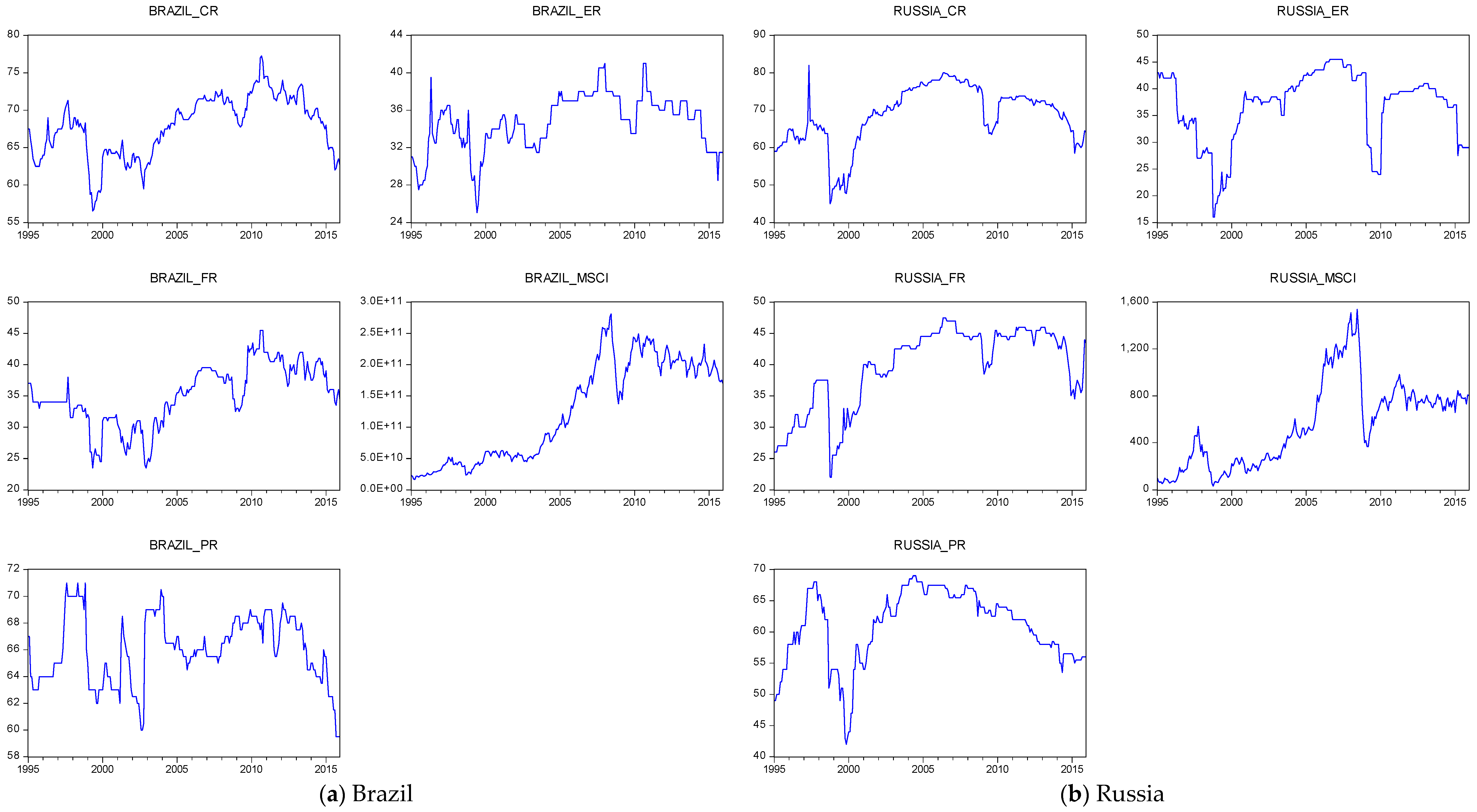
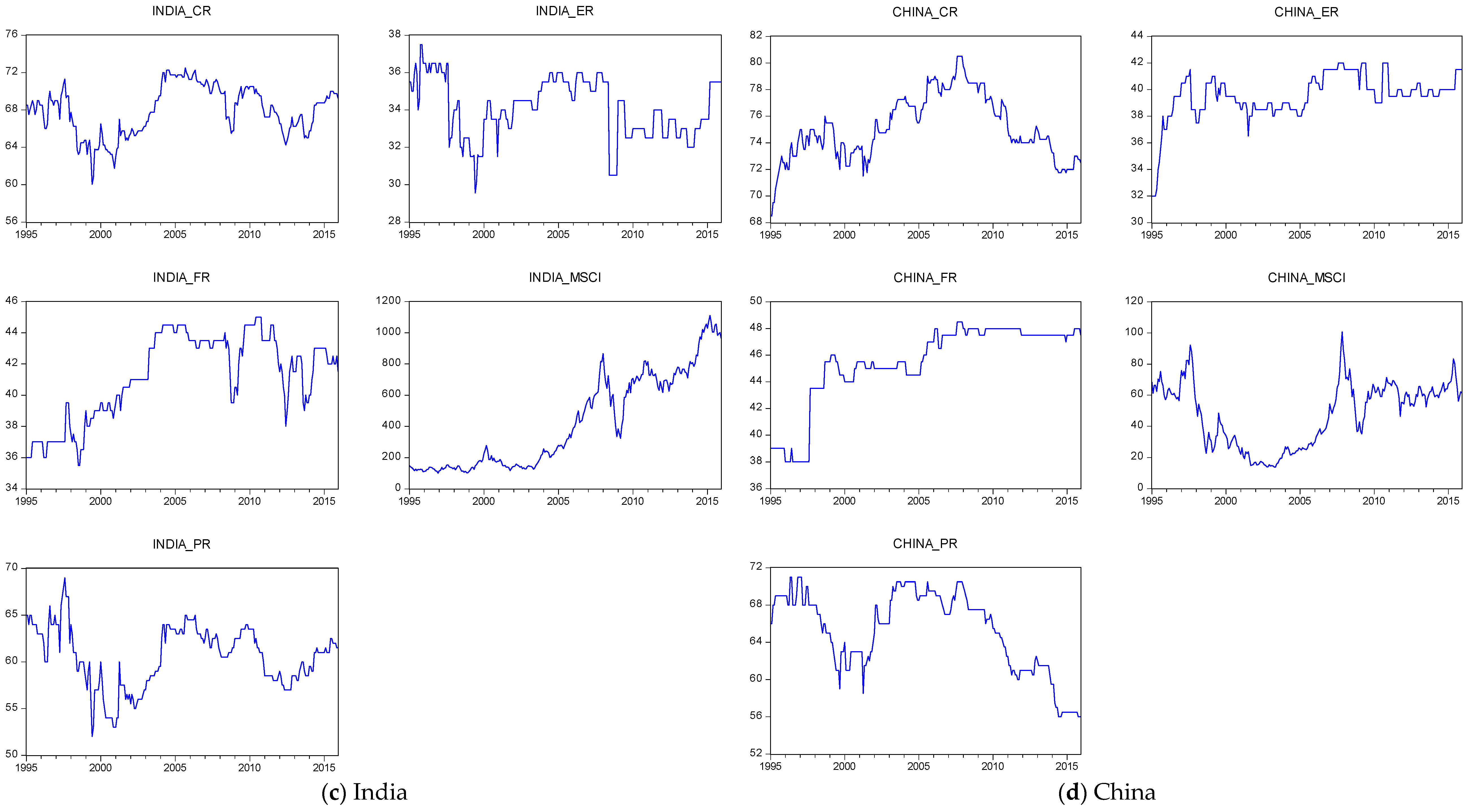
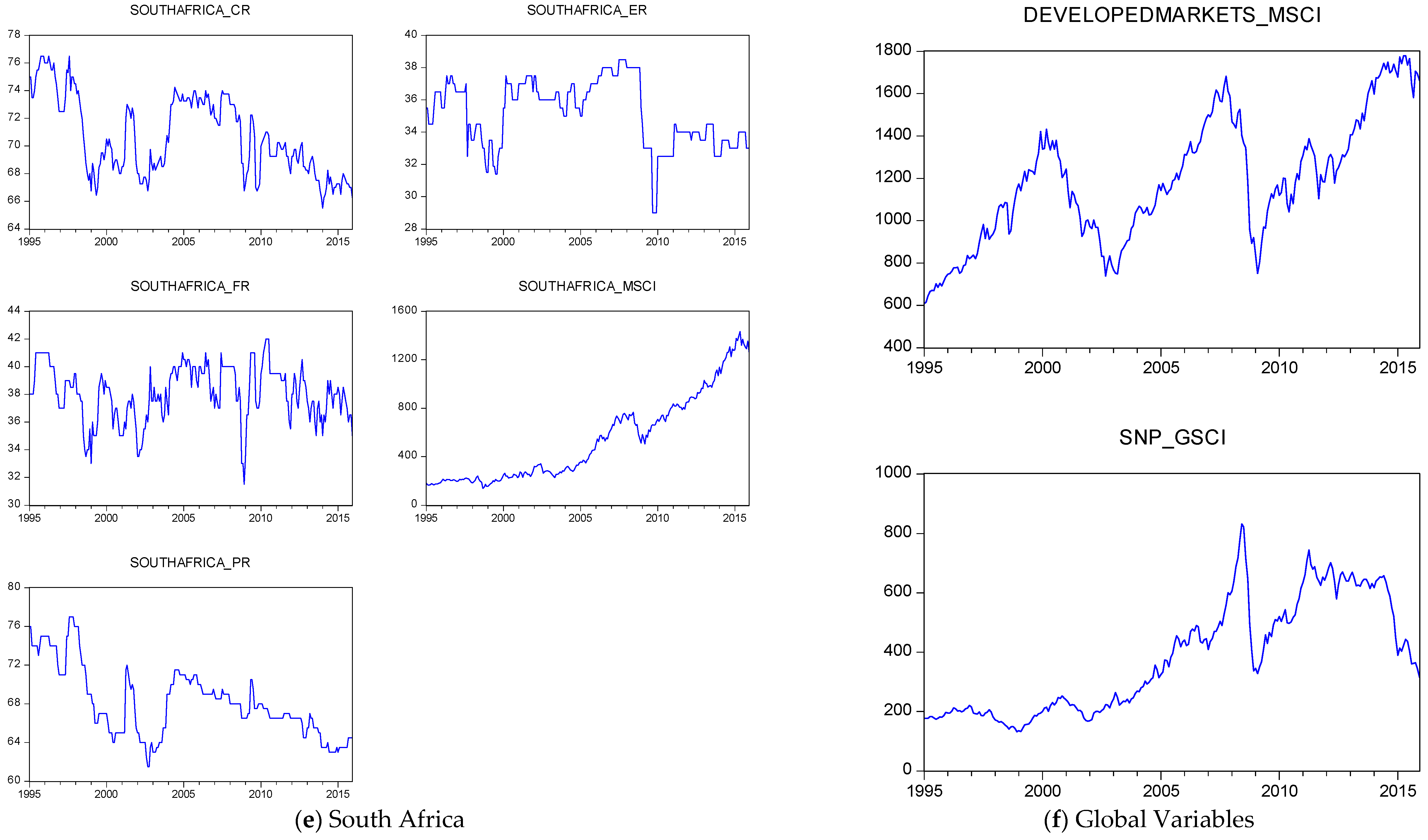
4.1. Data

We use Political Risk Services (PRS)’s International Country Risk Guide (ICRG) composite, economic, financial, and political risk ratings for the five BRICS countries over the monthly period of January 1995 to December 2015 (i.e., a total of 252 monthly observations). For the same period and frequency, we sourced the MSCI developed countries stock index and the dollar-denominated MSCI equity return indexes of the BRICS countries. Denominating the stock market indices in US dollars helps us to eliminate the effect of local inflation and national exchange rate fluctuations. We also use the S&P GSCI commodity spot price index, since these markets are large consumers and producers in the global commodity markets. Note the same start and end periods across the BRICS countries are determined purely by data availability and to ensure the comparability of results based on the sample size.
The ICRG of PRS creates the composite country risk ratings comprised of the political risk (PR) ratings; financial risk (FR) ratings; and, economic risk (ER) ratings. The PR accounts for 50% of the composite risk ratings, while each of the other two ratings have a weight of 25% each of the composite. It is important to note that the greater the number of points assigned for a risk rating factor, the lower the risk measured by that factor. The PR rating group identifies 12 political risk indicators covering government stability to conflict, corruption, democracy, and bureaucracy. The five indicators with the highest weight and assigned 12 points each are: Government Stability; Socioeconomic Conditions; Investment Profile; Internal Conflict; and, External Conflict. All of the remaining indicators have six points each, barring, Bureaucracy Quality, which is assigned four points. The total number of points for the PR group is 100. The FR group includes five financial risk indicators, with each of them assigned 10 points to make up a total of 50 points. The five indicators are: Foreign Debt Service/GDP; Current Account/Exports of Goods and Services; Months of Imports Cover; and, Exchange Rate Stability. Finally, the ER group also includes five economic risk indicators, with a total point of 50 also assigned for this group like the FR group. The five ER indicators are: GDP per Capita; Real GDP Growth, Annual Inflation Rate; Budget Deficit/GDP; and, Current Account/GDP.
Figure A1 in the Appendix A presents the time-series graphs of the data used in the study. The first five graphs show the risk ratings in the BRICS countries. The risk rating levels and variations differ from one country to another. In particular, the composite, economic, and financial risk ratings for China exhibit remarkably low variation over time, especially from 1998 onwards. Unlike China, Russia’s risk ratings exhibit much greater variation. Examining the stock price dynamics of developed and BRICS markets as well as the S&P GSCI commodity spot price index, we generally observe that all BRICS countries have experienced an upward trend in their stock market indices over the whole sample period, with the exception of China.
The descriptive statistics presented in Table A1 in the Appendix A show that the highest mean and median values in composite, economic and financial risk ratings are observed in the case of China, while the highest mean and median values of political risk rating are observed in South Africa. Therefore, the comparison of the mean values for country ratings suggests that, among the BRICS countries, China is the least economically and financially risky country, while South Africa is the least politically risky country. On the other hand, Brazil has the lowest mean and median values in terms of composite and financial risk ratings, while India experiences the lowest mean and median values for both economic and political risk ratings. These observations suggest that Brazil is the most financially risky country while India is the most economically and politically risky country. However, when examining the coefficient of variation values, i.e., the ratio of standard deviation to mean, we can see that the higher values are observed in Russia for all four risk categories, suggesting that Russia experiences the highest historical volatility for all country risk ratings, possibly making it harder for global investors to come up with economic forecasts for this major economy.
We also observe that almost all of the risk ratings series have negatively skewed distributions (except China for the composite risk index and South Africa for both composite and political risk indexes), indicating that greater probability of large increases in risk levels (i.e., decreases in risk ratings) than decreases. Significant high kurtosis values are observed only for China’s economic and financial risk ratings, implying fatter tails than a normal distribution for these two risk measures, while significant low values are obtained for India’s composite and financial risk ratings, China’s political risk rating and South Africa’s composite risk rating. This implies that the distribution of the above-mentioned risk factors is concentrated towards the mean and it has skinny tails. These observations are further supported by the JB statistics, indicating a rejection of the normality assumption at the conventional significance levels for the four risk factors in all BRICS countries, except for China’s composite risk rating.
Additionally, in Table A2, while using standard unit root tests, namely the Augmented (Dickey and Fuller 1979), (ADF), (Phillips and Perron 1988) (PP), and (Ng and Perron 2001), (NP), we show that none of the variables that were used in the analysis are integrated of order 2, i.e., I(2). This is an important result, as ARDL-types models does not allow for I(2) variables in the system.

4.2. Empirical Results from the NARDL Models

We begin our analysis by testing the presence of the long-run cointegrating relationship among variables in Models 1–6, as presented in Equations (4)–(9). As mentioned earlier, we test the significance of the lagged levels of the variables in each underlying NARDL model while using the F-statistic (denoted as FPSS test), where the null hypothesis of no cointegration is that the coefficients on the level variables are jointly equal to zero. Table 1 reports the results of the FPSS tests for each model across the BRICS stock markets presented in different columns.
Examining the results for Model 2 in Equation (5) where the stock market index is the dependent variable, we observe that the FPSS test statistics are highly significant, only in the case of China and Russia, implying a long-run equilibrium relationship between the stock market index, the commodity index, the MSCI developed country index, and the positive and negative changes in the economic, financial, and political risk ratings. On the other hand, when the political risk rating is used as a dependent variable, we observe evidence of a long-run cointegrating relationship for Brazil, India, and Russia only, while the same result holds for Brazil, India, and South Africa when financial risk rating is the dependent variable. However, taking the economic risk rating as a dependent variable produces evidence of a long-run relationship for all BRICS countries, except China. These findings suggest that BRICS countries exhibit quite a degree of heterogeneity in the interaction of their stock market returns with country-specific financial, political, and economic risk factors, while the most prevalent effects are observed in the case of China and Russia. Given the earlier observations that China is the least economically and financially risky country in the sample and Russia experiences the highest historical volatility for all country risk ratings, these findings suggest the level of risk for a given country or its stability over time is not necessarily the primary determinant of its stock market’s sensitivity to rating changes and other economic factors might be at play. At the same time, quite a degree of interaction is observed across country risk factors as well, particularly for Brazil and India, consistently across the financial, political, and economic risk rating factors.
In the case of commodity returns specified as the dependent variable, as shown in Model 1, we observe a long-run cointegrating relationship in the case of Brazil, China and Russia only. This is not unexpected as these countries represent major exporters and importers in our sample. Sudden shocks in the country-specific risk factors for these major players can significantly affect the commodity return dynamics. Interestingly, however when the MSCI developed stock market index is the dependent variable (Model 6), Brazil and Russia drop out and are replaced by South Africa, implying greater integration of this BRICS nation along with China with the world stock markets. While it is not surprising to observe a significant interaction between positive and negative changes in country specific risk factors for China and global stock market movements as this country is a key catalyst for global market dynamics, it is interesting that South Africa also yields significant results, possibly due to the degree of integration of this emerging market with global stock markets. Next, we examine the findings for the NARDL models.
The estimation results for the NARDL models for each BRICS stock market are presented in Table 2. As noted earlier, the main focus of this study is the possible existence of both long-run and short-run asymmetries in the response of BRICS stock market returns to positive and negative changes in risk rating factors. For this purpose, we report for each country only the estimation results for Model 2 in Equation (5) where the stock market return is the dependent variable. The results for the remaining models are not reported for brevity and they are available upon request. As noted earlier in the model description, L x + and L x ( x = P ,   F and E ) are the asymmetric positive and negative long-run coefficients and L C M and L S D are the symmetric long-run coefficients for the commodity and global stock markets. We use the Wald test statistic denoted by W L R x in the table to test long-run symmetry that is represented by the null hypotheses H 0 :   L x + = L x . Similarly, W S R x is the short-run asymmetry test statistic based on the Wald test for the additive short-run symmetry formulated by the null hypothesis: H 0 : j = 0 q 1 φ x , j + = j = 0 q 1 φ x , j .
The BDM test based on the co-integration test statistic by Banerjee et al. (1998) confirms the earlier FPSS test results, indicating cointegration in all the considered equations for each country, with the exception of Model 2 for Russia and Model 6 for China and South Africa7. Examining the symmetric long-run coefficients in Table 2, we observe quite a degree of heterogeneity across the BRICS stock markets. One commonality, though, is that the commodity market seems to have a more consistent long-run equilibrium relationship with BRICS stock markets when compared to that with developed stock markets, implied by significant estimates for LCM across all BRICS markets with the exception of Brazil. This confirms our prior argument that commodity market movements indeed act as a systematic catalyst for stock market movements in this bloc of major global importer and exporters. Interestingly, the LCM values are estimated to be positive regardless of the importer or exporter classification, implying a positive long-run relationship between the commodity and BRICS stock markets. When considering that oil carries a significant weight in the commodity index, a positive trend in commodity markets may indicate an improving demand for energy (and other raw materials for production) due to favorable global economic fundamentals, which also means good news for emerging countries as investors would be more willing to divert their funds into emerging stock markets in order to ride the wave of global growth expectations. On the other hand, a significant long-run equilibrium relationship with developed stock markets is only observed in the case of India, with weaker results for South Africa. These observations imply that, in the long-run, the commodity market acts as a catalyst for these emerging stock markets as opposed to developed stock markets.
Looking at the asymmetric impact of country rating changes, once again, we observe that BRICS stock markets exhibit heterogeneity in their long-run relationship with country risk ratings, with the strongest asymmetric effects being observed in the case of China. We generally reject symmetry in both the short- and long-run, implying that positive and negative changes in political, financial, and economic risk ratings yield an asymmetric impact on stock market returns. We also observe that negative changes in the country risk ratings generally command higher coefficient estimates in absolute value, implying the greater impact of bad news on stock market dynamics. This can be a manifestation of informational inefficiencies plaguing these emerging markets as investors over-react to bad news, either due to possible herding effects that are more prevalent during bad times or due to loss aversion by investors.
Focusing on the findings for China, we see that shocks in political and financial ratings have a negative long-run effect on its stock market return, regardless of the sign of the shock, as implied by negative estimates for LP+, LP−, LF+, and LF− for this country. The negative effect on the stock market may be a manifestation of the increased uncertainty these shocks bring to the market as retail investors who dominate this emerging stock market scramble to make sense of what the rating change truly means in terms of future growth expectations. In fact, we observe a similar negative effect of rating changes in the case of Russia and partially in South Africa as well, regardless of the sign of the change. To that end, the prevalent negative effect of financial and political rating changes may be due to informational inefficiencies in the stock market that hinders the processing of new information in a fundamental way, thus leading investors to take a cautious stand in their investments.
Finally, we do not observe any significant asymmetric effects of rating changes in the case of Brazil and India. The insignificant results that were observed for India are, in fact, consistent with the recent finding by Balcilar et al. (2017) that India is the most resilient BRIC nation to geopolitical risks with no significant causality effects observed on its stock market returns. Overall, our findings point to heterogeneity in the way BRICS stock markets react to country risk rating changes with the strongest effects observed in the case of China and in the case of negative rating changes. Furthermore, we observe the effect of these rating changes are not limited to stock markets only, but spills over to the commodity market as well.8

5. Conclusions

This study examines the interactions of stock market returns with country risk ratings and global risk factors via a Non-linear Auto Regressive Distributed Lags (NARDL) specification that allows for testing the presence of asymmetric effects in the short- and long-run relationships. We capture asymmetric cointegration by differentiating between positive and negative changes in country-specific risk factors measured by the political, financial, and economic risk ratings. Focusing on the major emerging stock markets in the BRICS, we analyze the linkages between local stock market returns, country risk ratings, and international factors, including commodity and developed stock markets.
Our findings suggest that BRICS countries exhibit quite a degree of heterogeneity in the interaction of their stock markets with country-specific financial, political, and economic risk factors, while the most prevalent effects are observed in the case of China. We observe that symmetry, in both the short- and long-run, is largely rejected for all country-specific risk factors, suggesting that positive and negative changes in political, financial, and economic risk ratings yield an asymmetric impact on stock market returns as well as global variables, particularly commodity returns. While some degree of heterogeneity is observed in how financial, economic and political risk ratings interact in the long-run, our findings suggest that positive and negative rating changes in some BRICS countries have significant implications for both local stock market returns as well as commodity price dynamics. Particularly, the Chinese stock market stands out in its long-run equilibrium relationship with country rating changes, while no significant effects are observed for India and Brazil.
Interestingly, shocks in financial and political ratings are found to have negative long-run effects on BRICS stock returns, regardless of the sign of the shock, while an opposite effect is observed for economic ratings. While some of the results can be attributed to the informational inefficiencies and mis-pricing present in these stock markets, our findings clearly suggest that not all BRICS nations are the same in terms of how they react to ratings changes and how they interact with global market indicators. From an investment perspective, our findings can be used as a guideline for global investors in their market timing strategies towards emerging stock markets, as well as in their predictive models for commodity markets.
It is important to point out that the variables incorporated in the econometric framework are in line with earlier research in this area, and it is parsimonious in nature. As part of future research, it would be interesting to extend our analysis by incorporating possible other predictors of the BRICS stock returns, as suggested by Sousa et al. (2016) in our current model, and check for the robustness of our results.

Author Contributions

Conceptualization, J.C., D.R. and R.G.; Methodology, A.B.N. and R.G.; Software, A.B.N.; Writing- Original Draft Preparation, J.C., D.R. and R.G.; Writing-Review & Editing: J.C., D.R. and R.G.

Funding

This research was funded by Ministerio de Economia y Competitividad, Spain (ECO2017-83183-R).

Acknowledgments

We would like to thank three anonymous referees for many helpful comments. Any remaining errors are solely ours.

Conflicts of Interest

The authors declare no conflict of interest.

Appendix A. Detailed Specification of the NARDL Models Estimated

The NARDL Models

The NARDL Models provided in Equations (4)–(9) can be presented in detailed form as
Δ C M t = c + ρ C M t 1 + θ S S t 1 + θ SD SD t 1 + θ P +   P t 1 + + θ P   P t 1 + θ F +   F t 1 + + θ F   F t 1 + θ E +   E t 1 + + θ E   E t 1 + i = 1 p 1 γ i Δ C M t i + j = 0 q 1 φ S , j Δ S t j + j = 0 q 1 φ S D , j Δ S D t j + j = 0 q 1 ( φ P , j +   Δ P t j + + φ P , j   Δ P t j ) + j = 0 q 1 ( φ F , j +   Δ F t j + + φ F , j   Δ F t j ) + j = 0 q 1 ( φ E , j +   Δ E t j + + φ E , j   Δ E t j ) + ε t
Δ S t = c + ρ S t 1 + θ C M C M t 1 + θ SD SD t 1 + θ P +   P t 1 + + θ P   P t 1 + θ F +   F t 1 + + θ F   F t 1 + θ E +   E t 1 + + θ E   E t 1 + i = 1 p 1 γ i Δ S t i + j = 0 q 1 φ C M , j Δ C M t j + j = 0 q 1 φ S D , j Δ S D t j + j = 0 q 1 ( φ P , j +   Δ P t j + + φ P , j   Δ P t j ) + j = 0 q 1 ( φ F , j +   Δ F t j + + φ F , j   Δ F t j ) + j = 0 q 1 ( φ E , j +   Δ E t j + + φ E , j   Δ E t j ) + ε t
Δ P t = c + ρ P t 1 + θ S S t 1 + θ SD SD t 1 + θ C M C M t 1 + θ F +   F t 1 + + θ F   F t 1 + θ E +   E t 1 + + θ E   E t 1 + i = 1 p 1 γ i Δ P t i + j = 0 q 1 φ S , j Δ S t j + j = 0 q 1 φ C M , j Δ C M t j + j = 0 q 1 φ S D , j Δ S D t j + j = 0 q 1 ( φ F , j +   Δ F t j + + φ F , j   Δ F t j ) + j = 0 q 1 ( φ E , j +   Δ E t j + + φ E , j   Δ E t j ) + ε t
Δ F t = c + ρ F t 1 + θ S S t 1 + θ SD SD t 1 + θ C M C M t 1 + θ P +   P t 1 + + θ P   P t 1 + θ E +   E t 1 + + θ E   E t 1 + i = 1 p 1 γ i Δ F t i + j = 0 q 1 φ S , j Δ S t j + j = 0 q 1 φ C M , j Δ C M t j + j = 0 q 1 φ S D , j Δ S D t j + j = 0 q 1 ( φ P , j +   Δ P t j + + φ P , j   Δ P t j ) + j = 0 q 1 ( φ E , j +   Δ E t j + + φ E , j   Δ E t j ) + ε t
Δ E t = c + ρ E t 1 + θ S S t 1 + θ SD SD t 1 + θ C M C M t 1 + θ F +   F t 1 + + θ F   F t 1 + θ P +   P t 1 + + θ P   P t 1 + i = 1 p 1 γ i Δ E t i + j = 0 q 1 φ S , j Δ S t j + j = 0 q 1 φ C M , j Δ C M t j + j = 0 q 1 φ S D , j Δ S D t j + j = 0 q 1 ( φ F , j +   Δ F t j + + φ F , j   Δ F t j ) + j = 0 q 1 ( φ P , j +   Δ P t j + + φ P , j   Δ P t j ) + ε t
Δ S D t = c + ρ S D t 1 + θ S S t 1 + θ CM C M t 1 + θ P +   P t 1 + + θ P   P t 1 + θ F +   F t 1 + + θ F   F t 1 + θ E +   E t 1 + + θ E   E t 1 + i = 1 p 1 γ i Δ S D t i + j = 0 q 1 φ S , j Δ S t j + j = 0 q 1 φ C M , j Δ C M t j + j = 0 q 1 ( φ P , j +   Δ P t j + + φ P , j   Δ P t j ) + j = 0 q 1 ( φ F , j +   Δ F t j + + φ F , j   Δ F t j ) + j = 0 q 1 ( φ E , j +   Δ E t j + + φ E , j   Δ E t j ) + ε t
where S is the stock index, P is the political risk rating factor, F is the financial risk rating factor, E is the economic risk rating factor, CM is the commodity index and SD is the MSCI developed country index. All variables are measured in natural logarithm. The coefficients ρ   and   θ s , s = C M , S D   and   S , are the symmetric long-run coefficients. θ a +   and   θ a ,   a = P , F   and   E , are the asymmetric long-run coefficients. φ s , j , s = C M , S D   and   S , are the symmetric short-run coefficients while φ a , j +   and   φ a , j ,   a = P , F   and   E , are the asymmetric short-run coefficients of the NARDL model. γ i is the autoregressive parameter and ε t is i.i.d. zero mean random variables with finite variance σ ε 2 . Since the data is on monthly frequency, the maximum order of the lags in the NARDL model is chosen to be 12.
Figure A1. Times series plot of data.
Risks 06 00094 g0a1aRisks 06 00094 g0a1bRisks 06 00094 g0a1c
Table A1. Summary Statistics for country ratings.
VariablesMeanMedianMaximumMinimumStandard DeviationCVSkewnessKurtosisJarque-BeraProbability
Brazil_CR67.85568.25077.25056.5404.0610.060−0.3752.6247.3820.025
Brazil_ER34.65535.00041.00025.0602.9880.086−0.4873.13910.1790.006
Brazil−FR35.05035.00045.50023.5004.8490.138−0.3182.5836.0850.048
Brazil_PR66.00066.00071.00059.5002.5460.039−0.2462.4755.4380.066
Brazil_MSCI1.25 × 10111.12 × 10112.81 × 10111.66 × 10108 × 10100.6400.1421.42526.9100.000
Russia_CR68.71770.00082.00045.0007.8200.114−0.8293.34230.1010.000
Russia_ER36.83038.50045.50016.0006.6390.180−1.0483.41047.8480.000
Russia_FR39.57942.50047.50022.0006.4390.163−0.8712.55433.9340.000
Russia_PR60.89362.00069.00042.0005.7680.095−0.8183.32929.2580.000
Russia_MSCI554.690520.8461539.35431.221362.0810.6530.4862.44513.1410.001
India_CR67.90968.50072.50060.0302.6220.039−0.3012.3298.5140.014
India_ER34.09134.00037.50029.5601.6000.047−0.3182.4177.8280.020
India_FR41.16141.50045.00035.5002.7220.066−0.4341.89820.6670.000
India_PR60.53661.00069.00052.0003.2520.054−0.2742.5805.0070.082
India_MSCI424.631287.2421111.045100.851300.4120.7070.5351.89224.9420.000
China_CR75.08774.62580.50068.5002.4140.0320.1362.5013.3960.183
China_ER39.54139.50042.00032.0001.7130.043−1.7148.717466.5710.000
China_FR45.43546.00048.50038.0003.0400.067−1.4023.94791.9730.000
China_PR65.17766.00071.00056.0004.2540.065−0.5752.27419.4340.000
China_MSCI47.75154.250100.66213.75220.5370.430−0.0841.89413.1470.001
South Africa_CR70.69970.00076.50065.5002.8340.0400.2621.86616.4010.000
South Africa_ER35.14135.50038.50029.0002.0470.058−0.3732.6067.4760.024
South Africa_FR38.06938.00042.00031.5001.9960.052−0.4932.95510.2360.006
South Africa_PR68.13967.50077.00061.5003.6400.0530.5582.58514.8610.001
South Africa_MSCI538.146375.2841432.465137.224355.2190.6600.7892.50128.7380.000
Developed Markets_MSCI1184.7461178.4201779.307608.263294.2150.2480.1732.2257.5590.023
S&P GSCI Commodity Spot Price Index379.791348.328832.304131.751188.5180.0600.4221.80122.5870.000
Note: The table presents the summary statistics for monthly composite (CR), economic (ER), financial (FR) and political (PR) risk ratings for the five BRICS countries over the period of January 1995 to December 2015. x_MSCI represents the stock market index for country x. CV is the coefficient of variation.
Table A2a. Unit root test results.
(a)
Level
VariableADFPPNP
ConstantConstant + TrendConstantConstant + TrendConstantConstant + Trend
Brazil_CR−1.635−1.545−1.911−1.934−6.016 *−6.334
Brazil_ER−2.936 **−2.905−2.928 **−2.956−7.940 *−16.03 *
Brazil−FR−2.188−2.875−2.241−2.982−8.000 *−8.716
Brazil_PR−2.412−2.355−2.412−2.355−12.28 **−13.283
Brazil_MSCI−1.637−1.519−1.637−1.5770.335−6.310
Russia_CR−2.214−2.104−2.141−2.017−4.184−8.738
Russia_ER−2.445−2.481−2.512−2.555−7.393 *−9.486
Russia_FR−2.480−2.570−2.523−2.803−0.632−7.984
Russia_PR−2.476−2.290−2.666−2.484−1.742−4.058
Russia_MSCI−2.243−2.842−1.940−2.692−1.225−14.669 *
India_CR−2.417−2.545−2.364−2.495−10.926 **−11.185
India_ER−3.783 **−3.795 **−3.804 **−3.822 **−17.008 ***−25.341 ***
India_FR−2.243−2.527−2.316−2.381−1.110−10.360
India_PR−2.860 *−2.832−2.682 *−2.642−6.229 *−10.682
India_MSCI−0.468−2.762−0.538−2.9710.710−6.805
China_CR−2.794 *−2.458−2.795 *−2.414−0.849−2.081
China_ER−4.749 ***−4.722 ***−4.749 ***−4.715 ***−0.050−3.565
China_FR−2.071−2.070−2.064−2.054−0.019−5.740
China_PR−0.746−1.678−0.514−1.529−1.993−4.984
China_MSCI−1.530−1.913−1.629−1.983−2.706−3.213
South Africa_CR−2.619 *−3.141 *−2.523−3.042−2.726−18.075 **
South Africa_ER−2.701 *−2.966−2.688 *−3.007−13.943 ***−16.045 *
South Africa_FR−4.291 ***−4.280 ***−4.426 ***−4.414 ***−33.194 ***−32.647 ***
South Africa_PR−2.308−2.538−2.424−2.766−0.797−8.168
South Africa_MSCI−0.330−3.067−0.242−3.0791.254−10.501
Developed Markets_MSCI−2.122−2.383−2.261−2.7190.425−4.964
S&P GSCI Commodity Spot Price Index−1.513−1.280−1.484−1.280−1.277−8.470
***, **, * indicates rejection of null hypothesis at 1%, 5%, and 10% level of significance respectively.
(b)
First Difference
VariableADFPPNP
ConstantConstant + TrendConstantConstant + TrendConstantConstant + Trend
Brazil_CR−13.954 ***−13.945 ***−13.954 ***−13.945 ***−123.228 ***−123.077 ***
Brazil_ER−10.699 ***−10.739 ***−16.416 ***−16.420 ***−265.278 ***−267.574 ***
Brazil−FR−15.371 ***−15.341 ***−15.371 ***−15.341 ***−124.937 ***−124.842 ***
Brazil_PR−14.366 ***−14.360 ***−14.334 ***−14.315 ***−123.935 ***−123.979 ***
Brazil_MSCI−15.810 ***−15.874 ***−15.810 ***−15.875 ***−40.119 ***−124.007 ***
Russia_CR−16.831 ***−16.835 ***−16.874 ***−16.852 ***−124.450 ***−124.437 ***
Russia_ER−16.339 ***−16.306 ***−16.351 ***−16.318 ***−124.834 ***−124.831 ***
Russia_FR−12.357 ***−12.390 ***−13.274 ***−13.267 ***−183.011 ***−183.631 ***
Russia_PR−15.790 ***−15.868 ***−15.866 ***−15.911 ***−124.999 ***−124.997 ***
Russia_MSCI−13.629 ***−13.630 ***−13.590 ***−13.588 ***−7.48776 *−19.8712 **
India_CR−15.429 ***−15.402 ***−15.527 ***−15.498 ***−124.950 ***−124.927 ***
India_ER−16.408 ***−16.387 ***−16.924 ***−17.230 ***−124.790 ***−124.786 ***
India_FR−13.688 ***−13.706 ***−13.564 ***−13.571 ***−122.614 ***−121.793 ***
India_PR−13.109 ***−13.102 ***−16.686 ***−16.715 ***−170.486 ***−170.648 ***
India_MSCI−14.741 ***−14.719 ***−14.747 ***−14.725 ***−29.557 ***−122.479 ***
China_CR−16.489 ***−16.718 ***−16.482 ***−16.758 ***−124.748 ***−124.688 ***
China_ER−16.083 ***−16.155 ***−16.083 ***−16.155 ***−124.963 ***−124.952 ***
China_FR−16.172 ***−16.215 ***−16.174 ***−16.225 ***−124.944 ***−124.966 ***
China_PR−17.253 ***−17.316 ***−17.379 ***−17.545 ***−124.009 ***−123.866 ***
China_MSCI−14.061 ***−14.066 ***−14.015 ***−14.008 ***−5.917 *−116.973 ***
South Africa_CR−13.822 ***−13.793 ***−13.723 ***−13.689 ***−122.948 ***−122.651 ***
South Africa_ER−16.529 ***−16.501 ***−16.770 ***−16.741 ***−124.709 ***−124.705 ***
South Africa_FR−16.228 ***−16.201 ***−16.837 ***−16.801 ***−124.859 ***−124.986 ***
South Africa_PR−14.068 ***−14.054 ***−14.070 ***−14.056 ***−123.372 ***−123.397 ***
South Africa_MSCI−15.824 ***−15.792 ***−15.896 ***−15.899 ***−1.851−36.2192 ***
Developed Markets_MSCI−13.925 ***−13.917 ***−14.032 ***−14.022 ***−122.520 ***−123.040 ***
S&P GSCI Commodity Spot Price Index−11.018 ***−11.066 ***−11.069 ***−11.079 ***−110.133 ***−109.161 ***
***, **, * indicate rejection of null hypothesis at 1%, 5%, and 10% level of significance respectively.

References

  1. Ang, Andrew, and Geert Bekaert. 2004. How do regimes affect asset allocation? Financial Analyst Journal 60: 86–98. [Google Scholar] [CrossRef]
  2. Bekaert, Geert, and Campbell Harvey. 1997. Emerging equity market volatility. Journal of Financial Economics 43: 29–77. [Google Scholar] [CrossRef]
  3. Balcilar, Mehmet, Matteo Bonato, Riza Demirer, and Rangan Gupta. 2017. Geopolitical Risks and Stock Market Dynamics of the BRICS. Economic Systems 42: 295–306. [Google Scholar] [CrossRef]
  4. Banerjee, Anindya, Juan Dolado, and Ricardo Mestre. 1998. Error-correction mechanism tests for cointegration in a single-equation framework. Journal of Time Series Analysis 19: 267–83. [Google Scholar] [CrossRef] [Green Version]
  5. Bilson, Christopher M., Timothy J. Brailsford, and Vincent C. Hooper. 2002. The explanatory power of political risk in emerging markets. International Review of Financial Analysis 11: 1–27. [Google Scholar] [CrossRef]
  6. Caldara, Dario, and Matteo Iacoviello. 2016. Measuring Geopolitical Risk; Working Paper. Washington: Board of Governors of the Federal Reserve Board.
  7. De Santis, Giorgio, and Bruno Gérard. 1997. International asset pricing and portfolio diversification with time varying risk. Journal of Finance 52: 1881–912. [Google Scholar] [CrossRef]
  8. Dickey, David A., and Wayne A. Fuller. 1979. Distribution of the estimators for autoregressive times series with a unit root. Journal of the American Statistical Society 75: 427–31. [Google Scholar]
  9. Engle, Robert, and Clive Granger. 1987. Co-integration and error correction: Representation, estimation and testing. Econometrica 55: 251–76. [Google Scholar] [CrossRef]
  10. Erb, Claude B., Campbell R. Harvey, and Tadas E. Viskanta. 1994. National risk in global fixed-income allocation. Journal of Fixed Income 4: 17–26. [Google Scholar] [CrossRef]
  11. Erb, Claude B., Campbell R. Harvey, and Tadas E. Viskanta. 1995. Country risk and global equity selection. The Journal of Portfolio Management 21: 74–83. [Google Scholar] [CrossRef]
  12. Erb, Claude B., Campbell R. Harvey, and Tadas E. Viskanta. 1996. Political risk, economic risk, and financial risk. Financial Analysts Journal 52: 29–46. [Google Scholar] [CrossRef]
  13. Errunza, Vihang, and Etienne Losq. 1985. International asset pricing under mild segmentation: Theory and test. Journal of Finance 40: 105–24. [Google Scholar] [CrossRef]
  14. Forbes, Kristin, and Roberto Rigobon. 2002. No contagion, only interdependence: Measuring stock market comovements. The Journal of Finance 57: 2223–61. [Google Scholar] [CrossRef]
  15. Girard, Eric, and Mohamed Omran. 2007. What are the risks when investing in thin emerging equity markets: Evidence from the Arab world. Journal of International Financial Markets, Institutions and Money 17: 102–23. [Google Scholar] [CrossRef]
  16. Godfrey, Leslie. 1978. Testing for multiplicative heteroskedasticity. Journal of Econometrics 8: 227–36. [Google Scholar] [CrossRef]
  17. Granger, Clive W., and Gawon Yoon. 2002. Hidden Cointegration. 2002-02. San Diego: University of California. [Google Scholar]
  18. Greenwood-Nimmo, Matthew, Tae-Hwan Kim, Yongcheol Shin, and Till Van Treeck. 2013. Fundamental Asymmetries in US Monetary Policymaking: Evidence from a Nonlinear Autoregressive Distributed Lag Quantile Regression Model. Mimeo: University of Melbourne. [Google Scholar]
  19. Grubel, Herbert. 1968. Internationally diversified portfolios: Welfare gains and capital flows. American Economic Review 58: 1299–314. [Google Scholar]
  20. Hamilton, James D. 1983. Oil and the macroeconomy since WWII. Journal of Political Economy 91: 228–48. [Google Scholar] [CrossRef]
  21. Hammoudeh, Shawkat, Ramazan Sari, Mehmet Uzunkaya, and Tengdong Liu. 2013. The dynamics of BRICS’s country risk ratings and domestic stock markets, U.S. stock market and oil price. Mathematics and Computers in Simulation 94: 277–94. [Google Scholar] [CrossRef]
  22. Harms, Philipp. 2002. Political risk and equity investment in developing countries. Applied Economics Letters 9: 377–80. [Google Scholar] [CrossRef]
  23. Harvey, Campbell R. 1995a. Predictable risk and returns in emerging markets. Review of Financial Studies 8: 773–816. [Google Scholar] [CrossRef]
  24. Harvey, Campbell R. 1995b. The risk exposure of emerging equity markets. The World Bank Economic Review 9: 19–50. [Google Scholar] [CrossRef]
  25. Harvey, Campbell R. 2012. Allocation to Emerging Markets in a Globally Diversified Portfolio. Durham: Duke University. [Google Scholar]
  26. Hatemi-J, Abdulnasser. 2012. Asymmetric causality tests with an application. Empirical Economics 43: 447–56. [Google Scholar] [CrossRef]
  27. Jarque, Carlos M., and Anil K. Bera. 1980. Efficient tests for normality, homoscedasticity and serial independence of regression residuals. Economics Letters 6: 255–59. [Google Scholar] [CrossRef]
  28. Johansen, Søren, and Katarina Juselius. 1990. Maximum likelihood estimation and inference on cointegration—With applications to the demand for money. Oxford Bulletin of Economics and Statistics 52: 169–210. [Google Scholar] [CrossRef]
  29. Kaminsky, Graciela, and Sergio L. Schmukler. 2001. Emerging Markets Instability: Do Sovereign Ratings Affect Country Risk and Stock Returns? Policy Research Working Paper Series 2678; Washington: The World Bank. [Google Scholar]
  30. Kang, Wensheng, and Ronald A. Ratti. 2013. Oil shocks, policy uncertainty and stock market returns. Journal of International Financial Markets, Institutions and Money 26: 305–18. [Google Scholar] [CrossRef]
  31. Lehkonen, Heikki, and Kari Heimonen. 2015. Democracy, political risk and stock market performance. Journal of International Money and Finance 59: 77–99. [Google Scholar] [CrossRef]
  32. Lintner, John. 1965. The valuation of risk assets and the selection of risky investments in stock portfolios and capital budgets. The Review of Economics and Statistics 47: 13–37. [Google Scholar] [CrossRef]
  33. Liu, Tengdong, Shawkat Hammoudeh, and Mark A. Thompson. 2013. A momentum threshold model of stock prices and country risk ratings: Evidence from BRICS countries. Journal of International Financial Markets, Institutions and Money 27: 99–112. [Google Scholar] [CrossRef]
  34. Longin, Franҫois, and Bruno Solnik. 1995. Is the correlation in international equity returns constant: 1960–90? Journal of International Money and Finance 14: 3–26. [Google Scholar] [CrossRef]
  35. Longin, Franҫois, and Bruno Solnik. 2001. Extreme correlation of international equity markets. The Journal of Finance 61: 649–76. [Google Scholar] [CrossRef]
  36. Mensi, Walid, Shawkat Hammoudeh, Seong-Min Yoon, and M. Mehmet Balcilar. 2017. Impact of macroeconomic factors and country risk ratings on GCC stock markets: Evidence from a dynamic panel threshold model with regime switching. Applied Economics 49: 1255–72. [Google Scholar] [CrossRef]
  37. Mensi, Walid, Shawkat Hammoudeh, Juan Carlos Reboredo, and Duc Khuong Nguyen. 2014. Do global factors impact BRICS stock markets? A quantile regression approach. Emerging Markets Review 19: 1–17. [Google Scholar] [CrossRef]
  38. Mensi, Walid, Shawkat Hammoudeh, Seong-Min Yoon, and Duc Khuong Nguyen. 2016. Asymmetric linkages between BRICS stock returns and country risk ratings: Evidence from dynamic panel threshold models. Review of International Economics 24: 1–19. [Google Scholar] [CrossRef]
  39. Ng, Serena, and Pierre Perron. 2001. Lag length selection and the construction of unit root tests with good size and power. Econometrica 69: 1519–54. [Google Scholar] [CrossRef]
  40. Pesaran, Hashem M., Yongcheol Shin, and Richard J. Smith. 2001. Bounds testing approaches to the analysis of level relationships. Journal of Applied Econometrics 16: 289–326. [Google Scholar] [CrossRef] [Green Version]
  41. Phillips, Peter C., and Pierro Perron. 1988. Testing for a unit root in time series regression. Biometrika 75: 335–46. [Google Scholar] [CrossRef]
  42. Ramcharran, Harri. 2003. Estimating the impact of risks on emerging equity market performance: Further evidence on data from rating agencies. Multinational Business Review 11: 77–90. [Google Scholar] [CrossRef]
  43. Ramsey, J.B. 1969. Tests for specification errors in classical linear least squares regression analysis. Journal of the Royal Statistical Society: Series B 31: 350–71. [Google Scholar]
  44. Romilly, Peter, Song Haiyan, and Xiaming Liu. 2001. Car ownership and use in Britain: A comparison of the empirical results of alternative cointegration estimation methods and forecasts. Applied Economics 33: 1803–18. [Google Scholar] [CrossRef]
  45. Sari, Ramazan, Mehmet Uzunkaya, and Shawtak Hammoudeh. 2013. The Relationship between Disaggregated Country Risk Ratings and Stock Market Movements: An ARDL Approach. Emerging Markets Finance and Trade 49: 4–16. [Google Scholar] [CrossRef]
  46. Scholes, Myron S. 2000. Crisis and Risk Management. American Economic Review 90: 17–21. [Google Scholar] [CrossRef] [Green Version]
  47. Schorderet, Yann. 2001. Revisiting Okun’s Law: An Hysteretic Perspective. San Diego: University of California, Mimeo. [Google Scholar]
  48. Sharpe, William F. 1964. Capital asset prices: A theory of market equilibrium under conditions of risk. The Journal of Finance 19: 425–42. [Google Scholar]
  49. Shin, Yongcheol, Byungchul Yu, and Matthew Greenwood-Nimmo. 2014. Modelling asymmetric cointegration and dynamic multipliers in an ARDL framework. In Festschrift in Honor of Peter Schmidt. Edited by William C. Horrace and Robin C. Sickles. New York: Springer Science & Business Media. [Google Scholar]
  50. Sousa, Ricardo M., Andrew Vivian, and Mark E. Wohar. 2016. Predicting asset returns in the BRICs: The role of macroeconomic and fundamental predictors. International Review of Economics and Finance 41: 122–43. [Google Scholar] [CrossRef] [Green Version]
  51. World Bank. 2015. World Development INDICATORS. Washington: The World Bank. [Google Scholar]
1
In 2010, South Africa joined this group of countries and formed the BRICS.
2
Mensi et al. (2017) also used this approach to carry out a similar analysis for Gulf Cooperation Council (GCC) countries.
3
Sari et al. (2013) have also used the autoregressive distributed lag (ARDL) model to study the impact of country risk ratings on the Turkish stock market.
4
The parameter ρ is assumed to be negative in order to have a cointegration relationship among the variables.
5
According to Granger and Yoon (2002), two times series are hidden cointegrated if their positive and negative components are cointegrated with each other.
6
For the bounds testing procedure, two sets of critical values are provided. The upper critical bound assumes that there is a cointegration relationship among the variables, while the lower critical bound assumes that no cointegration relationship exists between the variables. If the F-statistic is greater than the upper level critical value, then the null hypothesis of no-cointegration is rejected (i.e., all variables are cointegrated). Conversely, if the computed F-statistic falls below the lower bound critical value, then the null hypothesis cannot be rejected (i.e., no cointegration). Finally, if the F-statistic falls between the bounds, the test is inconclusive.
7
Results of the BDM test for all equations are available upon request.
8
Based on the suggestions of an anonymous referee, in order to account for bearish and bullish stock markets, we also estimated a quantiles-based version of the NARDL model, i.e., a QNARDL model as developed by Greenwood-Nimmo et al. (2013). Our results, which are available upon request, however. suggested that estimates of the parameters of model are not statistically different across the various quantiles. This result is an indication of the fact that our NARDL model is not misspecified across bear and bull markets and the QNARDL model does not necessarily bring in new information in our context. Having said this, we must also be cautious of the fact that this result could purely be driven by our relatively small sample size, which is not large enough to handle the overparameterized QNARDL model.
Table 1. FPSS tests.
BrazilChinaIndiaRussiaSouth Africa
Model 14.097 **5.247 ***3.2925.192 ***2.772
Model 23.384 *6.581 ***1.7345.495 ***2.747
Model 34.935 ***2.9735.664 ***9.238 ***2.902
Model 48.381 ***3.2885.146 ***3.523 *6.833 ***
Model 54.113 **3.2834.816 ***8.649 ***5.230 ***
Model 63.3104.326 **2.0982.0404.573 **
Note: This table presents the results of the FPSS tests for the presence of a long-run cointegrating relationship among the variables in Models 1–6 provided in Equations (4)–(9). The null hypothesis of no cointegration is that the coefficients on the level variables in each respective model are jointly equal to zero. Pesaran et al. (2001) tabulate the critical values for the FPSS test for k = 5, as 3.35, 3.79, and 4.68 at 10, 5, and 1 percent levels, respectively.6 ***, ** and * represent significance at the 1, 5, and 10 percent levels, respectively.
Table 2. Nonlinear ARDL estimation results for stock market returns.
(a).  
(a).  
BrazilChinaIndia
VariableCoeff.S.E.VariableCoeff.S.E.VariableCoeff.S.E.
c 0.4640.511 c −0.0950.252 c −0.3700.239
S t 1 −0.0200.024 S t 1 −0.089 ***0.020 S t 1 −0.055 **0.027
C M t 1 0.044 *0.026 C M t 1 0.128 ***0.032 C M t 1 0.038 *0.023
S D t 1 −0.0330.026 S D t 1 −0.0550.042 S D t 1 0.067 *0.039
P t 1 + −0.1920.175 P t 1 + −0.2220.135 P t 1 + 0.0910.111
F t 1 + −0.134 **0.054 F t 1 + −0.339 *0.173 F t 1 + 0.339 *0.179
E t 1 + −0.0270.077 E t 1 + 0.563 *0.287 E t 1 + −0.2350.202
P t 1 −0.359 *0.202 P t 1 −0.590 **0.269 P t 1 0.0900.131
F t 1 −0.0750.102 F t 1 −0.6510.649 F t 1 0.2250.137
E t 1 −0.0620.088 E t 1 1.230 ***0.251 E t 1 −0.1230.114
Δ S t 1 −0.120 **0.048 Δ C M t 0.318 ***0.089 Δ S t 5 −0.125 **0.050
Δ S t 2 −0.111 **0.049 Δ C M t 4 −0.378 ***0.091 Δ S t 7 −0.124 **0.048
Δ C M t 0.179 **0.071 Δ C M t 7 −0.243 **0.093 Δ C M t 0.227 ***0.075
Δ S D t 1 1.144 ***0.092 Δ C M t 10 −0.250 ***0.090 Δ C M t 8 −0.218 ***0.075
Δ P t 6 + −0.838 **0.353 Δ S D t 1 1.142 ***0.114 Δ S D t 1 0.726 ***0.091
Δ P t 10 + 0.844 **0.349 Δ S D t 7 0.324 ***0.114 Δ S D t 4 0.190 **0.088
Δ P t 11 + 1.000 ***0.375 Δ S D t 8 0.338 ***0.114 Δ S D t 5 −0.235 ***0.088
Δ P t 12 + −0.712 **0.349 Δ P t 2 + 1.410 **0.552 Δ S D t 9 0.202 **0.089
Δ F t 1 + 0.373 **0.159 Δ F t 6 + 1.415 ***0.480 Δ P t 3 + −0.687 **0.295
Δ F t 11 + −0.391 ***0.149 Δ E t 10 + 1.098 **0.483 Δ P t 7 + 0.732 **0.293
Δ E t 3 + 0.407 **0.177 Δ F t 3 2.632 **1.185 Δ P t 9 + −0.792 ***0.296
Δ E t 6 + 0.574 ***0.204 Δ F t + 0.936 **0.442
Δ P t 1 0.969 **0.484 Δ F t 6 + 0.821 **0.401
Δ F t 7 0.430 ***0.162 Δ F t 10 + −1.049 ***0.386
Δ F t 11 0.860 ***0.185 Δ P t 11 1.106 ***0.337
Δ E t 3 0.447 **0.188 Δ F t 9 1.180 ***0.453
Δ E t 5 0.496 **0.196 Δ E t 0.519 **0.241
Δ E t 1 1.090 ***0.246
Δ E t 1 −0.633 ***0.234
Long−run effects Δ E t 12 −0.716 ***0.243
L C M 2.2142.436 L C M 1.434 ***0.391 L C M 0.688 **0.297
L S D −1.6602.726 L S D −0.6110.537 L S D 1.234 **0.501
L P + −9.62616.577 L P + −2.484 *1.357 L P + 1.6561.995
L F + −6.7059.345 L F + −3.803 **1.705 L F + 6.2014.793
L E + −1.3644.728 L E + 6.313 **2.983 L E + −4.3015.027
L P −18.02625.062 L P −6.618 *3.775 L P 1.6551.971
L F −3.7557.658 L F −7.3036.644 L F 4.1163.246
L E −3.1206.054 L E 13.790 ***4.067 L E −2.2442.079
Statistics and Diagnostics
B D M −0.818 B D M −4.537 ** B D M −2.040
W L R P 0.247[0.620] W L R P 1.275[0.260] W L R P 0.000[0.999]
W L R F 0.304[0.582] W L R F 0.292[0.589] W L R F 0.779[0.379]
W L R E 0.350[0.555] W L R E 2.963[0.087] W L R E 0.194[0.660]
W S R P 0.548[0.460] W S R P 6.518[0.011] W S R P 9.183[0.003]
W S R F 16.788[0.000] W S R F 0.919[0.339] W S R F 0.350[0.555]
W S R E 0.011[0.916] W S R E 5.161[0.024] W S R E 0.237[0.627]
R ¯ 2   0.524 R ¯ 2   0.466 R ¯ 2   0.518
S C ( 12 ) 13.373[0.342] S C ( 12 ) 15.598[0.210] S C ( 12 ) 8.053[0.781]
R R T 5.155[0.023] R R T 0.020[0.886] R R T 0.267[0.605]
J B 4.644[0.098] J B 31.498[0.000] J B 0.239[0.887]
H T 43.365[0.000] H T 0.122[0.727] H T 0.010[0.921]
(b).  
(b).  
RussiaSouth Africa
VariableCoeff.S.E.VariableCoeff.S.E.
c −0.2080.346 c 0.260 *0.143
S t 1 −0.103 ***0.029 S t 1 −0.119 ***0.027
C M t 1 0.132 ***0.038 C M t 1 0.028 *0.015
S D t 1 0.0170.055 S D t 1 0.032 *0.019
P t 1 + 0.0890.151 P t 1 + 0.0720.095
F t 1 + 0.1340.183 F t 1 + 0.0170.072
E t 1 + −0.226 **0.091 E t 1 + 0.164 *0.088
P t 1 0.1960.228 P t 1 0.206 *0.117
F t 1 −0.340 **0.138 F t 1 −0.122 *0.072
E t 1 0.0620.059 E t 1 0.171 **0.072
Δ S t 1 0.105 **0.049 Δ C M t 0.146 ***0.052
Δ S t 10 0.110 **0.044 Δ C M t 0.611 ***0.071
Δ C M t 0.242 **0.119 Δ P t + −0.708 **0.294
Δ S D t 1 1.355 ***0.155 Δ P t 4 + −0.660 **0.292
Δ P t 7 + −0.950 **0.422 Δ P t 9 + 0.970 ***0.296
Δ F t + −0.869 ***0.328 Δ P t 1 −1.029 **0.416
Δ F t 10 + −0.860 ***0.326 Δ P t 10 −1.083 **0.419
Δ E t 7 + 0.382 **0.177 Δ F t 3 −0.386 **0.162
Δ P t 2.624 ***0.433 Δ F t 5 0.353 **0.155
Δ F t 1.271 ***0.258 Δ E t 12 0.655 ***0.189
Δ F t 4 0.989 ***0.246
Δ F t 5 −1.049 ***0.302
Δ F t 8 −0.521 **0.234
Δ F t 12 −0.735 ***0.274
Δ E t 1 −0.519 ***0.137
Δ E t 3 0.424 ***0.127
Δ E t 5 0.557 ***0.163
Δ E t 10 0.288 **0.134
Long−run effects
L C M 1.289 ***0.351 L C M 0.236 **0.115
L S D 0.1680.509 L S D 0.269 *0.143
L P + 0.8691.356 L P + 0.6060.809
L F + 1.3051.701 L F + 0.1410.599
L E + −2.194 **0.983 L E + 1.374 *0.768
L P 1.9082.003 L P 1.730 *0.992
L F −3.304 *1.727 L F −1.024 *0.584
L E 0.6000.610 L E 1.434 ***0.533
Statistics and Diagnostics
F P S S 5.495 *** F P S S 2.747
B D M −3.598 B D M −4.488 **
W L R P 0.242[0.623] W L R P 1.997[0.159]
W L R F 4.252[0.040] W L R F 34.555[0.000]
W L R E 5.881[0.016] W L R E 0.007[0.932]
W S R P 31.652[0.000] W S R P 4.941[0.027]
W S R F 4.434[0.036] W S R F 0.020[0.887]
W S R E 1.053[0.306] W S R E 12.053[0.001]
R ¯ 2   0.617 R ¯ 2   0.487
S C ( 12 ) 12.230[0.427] S C ( 12 ) 9.651[0.647]
R R T 2.735[0.098] R R T 3.550[0.060]
J B 5.720[0.057] J B 3.491[0.175]
H T 0.334[0.564] H T 30.155[0.000]
Notes: L x + and L x are the asymmetric positive and negative long-run coefficients, with x = P, F and E. L C M and L S D are the symmetric long-run coefficients. W L R x denotes the Wald test for long-run symmetry by testing the null hypothesis H 0 :   L x + = L x . W S R x denotes the Wald test of the additive short-run symmetry by testing the null hypothesis: H 0 : j = 0 q 1 φ x , j + = j = 0 q 1 φ x , j . BDM refers to the co-integration test statistic by Banerjee et al. (1998). Pesaran et al. (2001) tabulate the critical values of tBDM, for k = 5, as −3.86, −4.19 and −4.79 at 10, 5, and 1 percent levels, respectively. R-Bar denotes the adjusted R-square. SC(k) refers to the Godfrey (1978) test for kth order serial correlation. RRT denotes the Ramsey (1969) RESET test of functional form. JB denotes the Jarque and Bera (1980) test statistic for normality. HT is the MicroFit test for heteroscedasticity. p-values for tests are given in square brackets. ***, ** and * represent significance at the 1, 5 and 10 percent levels respectively.

