Risk of Bankruptcy, Its Determinants and Models

Department of Accounting and Controlling, Faculty of Management, University of Prešov, Konštantínova 16, 080 01 Prešov, Slovakia
*
Author to whom correspondence should be addressed.
Risks 2018, 6(4), 117; https://0-doi-org.brum.beds.ac.uk/10.3390/risks6040117
Submission received: 3 September 2018
/
Revised: 19 September 2018
/
Accepted: 5 October 2018
/
Published: 11 October 2018
Abstract
:In this paper, the following research problem was addressed: Is DEA (Data Envelopment Analysis) method a suitable alternative to Altman model in predicting the risk of bankruptcy? Based on the above-mentioned research problem, we formulated the aim of the paper: To apply DEA method for predicting the risk of bankruptcy and to compare its results with the results of Altman model. The research problem and the aim of the paper follow the research of authors aimed at the application of methods which are appropriate for measuring business financial health, performance and competitiveness as well as for predicting the risk of bankruptcy. To address the problem, the following methods were applied: financial ratios, Altman model for private non-manufacturing firms and DEA method. When applying DEA method, we formulated input-oriented DEA CCR model. We found that DEA method is an appropriate alternative to Altman model in predicting the risk of possible business bankruptcy. The important conclusion is that DEA allows us to apply not only outputs but also inputs. Since prediction models do not include these indicators, DEA method appears to be the right choice. We recommend, especially for Slovak companies, to apply cost ratio when calculating risk of bankruptcy.
1. Introduction
Business failure is a characteristic feature of all economies. It has an impact on a business as well as its surroundings. Therefore, it is necessary to mind out the prediction of the risk of business failure.
The starting point for risk assessment is the issue of risk definition. There are different opinions on this issue, mainly from the historical as well as contemporary point of view. Domestic and foreign literature provides several definitions of risk.
The term “risk” comes from Arabic, and expresses an unexpected event. Risk is usually defined as something unstable, indefinite which is related to the course of phenomenon and disturbs its behavior.
Key definition of risk was introduced by Lowrance (1976); Šotić and Rajić (2015) who said that “risk is the measure of probability and the weight of undesired consequences”. According to Čunderlík (2004), risk is the expression of the degree of uncertainty in various forms. The risk is defined as the state of imperfect knowledge when the decision-maker is aware of the various possible consequences of his decision and is able to estimate the degree of probability that this or that result occurs (Buganová and Hudáková 2012). Businesses have to face certain risks, whether financial, commercial, informational or personal. According to Fetisovová et al. (2004), for each financial decision, it is necessary to consider not only its expected return, but also the risk associated with it. Risk is one of the most important limits that define the scope of financial decision-making (Marinič 2008). Special attention should be paid to the risk of long-term financial decisions. Risk is the chance to achieve above-average return on investment (Klučka 2006). In 2009, Tranchard (2018) provided the following definition of risk: “Risk is the effect of uncertainty on objectives”. Risk is the probability that actual results will deviate from planned (expected) ones, in both positive and negative meaning (Markovič 2010). Risk is the “uncertainty” in which we are able to quantify the probability of diverting actual conditions, processes or results from the expected values using different methods (mainly statistical). Theory defines risk as a possibility of positive or negative diversion. In practice, risk is understood only as a negative diversion.
The risk is higher the more the actual result can deviate from the expected one, in both positive and negative directions (Mařík et al. 2011). The risk can be expressed as a quantitative and qualitative threat, while it is characterized by the probability of the occurrence of risk situation which can culminate in the crisis of a system (Tej et al. 2013). Risk is a category that affects the existence and performance of a business (Koscielniak 2014). No economic entity or business can predict its economic and financial results only based on internal results, since every activity involves external and macroeconomic risks. External as well as internal risks are the determinants of corporate bankruptcy. However, the main determinant of bankruptcy is insolvency (Cisko and Klieštik 2013). Some studies on risk of bankruptcy consider negative profitability as a prerequisite for bankruptcy (Scott 1981; Lukason and Laitinen 2018). Bankruptcy can be caused by both liquidity and profitability, as well as other financial areas of business. This issue is addressed in the current paper.
The next part of the text is structured as follows. Section 2 is the literature review. This section describes selected studies on risk of bankruptcy. The main methods are Altman discriminatory analysis model and DEA model. At the end of this section, the research problem and the aim of the paper are formulated. Section 3 describes the research sample and applied methods. Among these methods, there is DEA model for one hotel and also the preview how to process this model in Excel Solver. Section 4 contains descriptive statistics of selected financial indicators, as well as the results of internal and external risks as the determinants of bankruptcy. In this section, there are also results of Altman modified model for non-manufacturing firms and the results of DEA model. Section 5 is a polemic on obtained results. Section 6 concludes the research and brings significant findings.
2. Literature Review
“Bankruptcy is a situation where the liabilities exceed the assets in the company, generally it happens due to under capitalization, not maintaining sufficient cash, sources are not utilized properly, management of activities is inefficient, sales decline, and market situation deteriorates.” (Venkataramana et al. 2012). “Bankruptcy follows payment default or a situation in which the debtor company becomes unable to repay its debts. Although bankruptcy is part of the market selection process and can be considered to be the consequence of a firm’s inability to survive market competition, it may entail multiple damaging repercussions, occasionally of significant scale, in terms of job losses, the destruction of assets and productive base” (Aleksanyan and Huiban 2016).
“Bankruptcy risk is a possibility of anticipated legal bankruptcy procedure, followed by unfavorable financial consequences such a loss resources or expecting income” (Rybak 2006). “The bankruptcy means risk that a firm will be unable to meet its debt obligations. This risk is also referred to as default or insolvency risk“ (Campbell 2012). According to Rybak (2006), “bankruptcy risk takes place at all stages of the company’s life cycle. Its appearance is an objective inevitability of manager’s activities which is conditioned by vagueness of surroundings and insufficiency of company’s resources. Bankruptcy risk is greater when the individual or firm has little or no cash flow, or when it manages its assets poorly. Banks assess bankruptcy risk when considering whether to make a loan“ (Campbell 2012).
“Prediction of bankruptcy risk is of increasing importance to corporate governance. Many different models have been used to predict corporate bankruptcy. These methods all have their particular strengths and weaknesses, and choosing between them for empirical application is not straightforward” (Aziz and Dar 2006).
“From the existing approaches to the bankruptcy prediction (accounting analytical approach, option theoretical approach and statistical approach), the statistical approach tries to asses’ corporate failure risk through four widely known methods which make use of balance-sheet ratios: linear or quadratic discriminant analysis, logistic regression analysis, probit regression analysis and neural network analysis. Many empirical researches adopt the statistical approach” (Becchetti and Sierra 2002).
First studies devoted to bankruptcy prediction were aimed at the application of financial ratios. Fitzpatrick identified significant differences between financially healthy and distressed businesses (Misankova and Bartosova 2016; Valášková et al. 2017). Research firstly focuses on univariate analysis. A major work in this area was the work of Beaver (1966). Beaver demonstrated that financial indicators can be useful in the prediction of an individual firm failure (Šarlija and Jeger 2011). He proved that not all financial indicators can be used to predict business failure. However, the use of simple financial indicators was questioned in practice because of their potential distortion by managerial decisions. Therefore, Beaver carried out the classification test using dichotomous prediction (Kidane 2004). With the use of this method, we can identify several financial indicators with the most predictive power that are used as a predictor with multiple degrees of freedom. Univariate analysis was later followed by authors who used multivariate analysis. In the beginning of prediction models, discriminant analysis was applied. The aim of this method is to find such linear combination of parameters which best distinguishes bankrupt and non-bankrupt businesses (Spuchľáková and Frajtová-Michalíková 2016). In 1968, Altman elaborated a multiple discriminant analysis model (MDA) known as the Z-Score model, and then he modified this model in 1983. Z-Score model has been the dominant model all over the world. Although it “has been in existence for more than 45 years, it is still used as a main or supporting tool for bankruptcy or financial distress prediction or analysis, both in research and practice” (Altman et al. 2014). During the next two decades, even more financial distress studies were realized; we can mention studies by Deakin (1972); Blum (1974); Moyer (1977); Springate (1978); Fulmer et al. (1984) and Ohlson (1980), who applied logit model; Taffler (1984) who developed model Z-score for United Kingdom; and Zmijewski (1984) who used a probit approach in his model and other authors. There are also many studies that examined the applicability and predictive power of pre-developed models, mainly Altman model. The study of Soon et al. (2014) confirmed that the use of Altman model as the predictor of financial failure of a company is a successful tool. Sulub (2014) found that Altman model is exact for the failed multinational companies at a predictive power of 70%, and for the non-failed at a predictive power of 55%. Reisz and Perlich (2007) assessed Altman model as a better measure for short-term bankruptcy prediction than the market-based models. Kidane (2004) in his study concluded that Altman and Springate model failed to predict failure and non-failure of service and information technology companies.
It is necessary to point out that “discriminant analysis is valid only under certain restrictive assumptions, including the requirement for the discriminating variables to be jointly multivariate normal. Logit regression is not subject to the restriction of normality” (Karels and Prakash 1987, Odom and Sharda 1990). Therefore, logit model, probit model and neural networks started to be used (Spuchľáková and Frajtová-Michalíková 2016). Logit model is used especially in those cases where the output variable is dichotomous (Klieštik et al. 2015). This model provides the ability to model complex relationships between variables (Adamko and Svabova 2016). The dichotomous dependent variable of a logit model is expressed by the logarithm of the probability that an event (fail/not-fail) will occur (Maddala 1983). Logit model uses cumulative distribution function of the logistic distribution. This model was applied by Liu et al. (2011) in identifying financial distress in a hospital. Probit model applies cumulative distribution function of the standard normal distribution (Albright 2015). In 2014, Altman introduced new model based on the application of discriminatory analysis and seven modifications of logit model. These models are applicable in the Slovak Republic. (Adamko and Svabova 2016). However, it should be noted that it is not possible to simply apply models in the conditions of other countries and different industries. In Slovakia and the Czech Republic, models based on the conditions of these countries have been formulated: Ch-index of Chrastinová (1998) processed for agricultural businesses and model of Gurčík (2002) designed to predict financial health of agricultural businesses.
Nowadays, neural networks are at the forefront of this issue. They eliminate the negatives of above-mentioned models. Neural networks bring new broader approach to solving the problem, which is based not only on the application of discriminatory variables. Neural network is comprehensive term for a set of procedures from the area of artificial intelligence. Some of these procedures can be used as classification systems. Neural networks are the alternative to discriminatory analysis. They do not require deep mathematical and statistical knowledge and do not need any assumptions. “Neural networks perform classification tasks in a way intended to emulate brain processes” (Salchenberger et al. 1992). The basis of neural network is neuron model with N inputs and M outputs. “The processing ability of the network is stored in the interunit connection strengths or weights, obtained by a process of adaptation to, or learning from, a set of training patterns” (Gurney 1997). Neural networks are used in regulatory and simulation techniques. The process of abstraction is called learning; it can be run with or without teacher. During this process, values of weights are updated. Several learning algorithms are described in the literature. Once learning is finished, weights do not change and the network produces outputs in accordance with the rules applied to the input values.
“Neural networks have proven to be good at solving many tasks”. The first attempt to use artificial neural networks (ANNs) to predict bankruptcy was made by Odom and Sharda (1990). “They may have the most practical effect in the following three areas: modelling and forecasting, signal processing, and expert systems” (Lippmann 1987, Odom and Sharda 1990). Based on the comparison of discriminatory analysis and neural networks, Odom and Sharda (1990) confirmed that neural networks are more appropriate tool for predicting bankruptcy. Rahimian et al. (1993) tested the same dataset used by Odom and Sharda with three neural network paradigms: backpropagation network, Athena and Perception. Several studies further investigate the use of ANNs in bankruptcy or business failure prediction. These studies conclude that ANNs are influential instruments for model recognition and classification due to their nonlinear nonparametric adaptive-learning properties (Kidane 2004).
Recently, there have been reviews on the efficacy of the models carried out by Agarwal and Taffler (2008); Das et al. (2009) and Bauer and Agarwal (2014). They consider the performance of accounting-based models, market-based models and hazard models, which dominate in the finance literature (Altman et al. 2014).
There are also another methods for bankruptcy prediction, we can mention decision trees – a form of supervised learning by generalizing from examples (Friedman 1977), Cash Management Theory aimed at short-term management of corporate cash balances (Black and Scholes 1973) and balance sheet decomposition measures based on the argument that firms try to maintain equilibrium in their financial structure (Booth 1983). In the prediction of bankruptcy Self – Organizing Map (SOM) is one of the frequently used models to analyse the high – dimensional financial data and understand the unwanted bankruptcy phenomenon. “The authors used SOM to analyse and visualise the financial situation of companies over several years through a two-step clustering process” (Chen et al. 2013). Very beneficial is study of Gherghina (2015). His empirical study was devoted to artificial intelligence (AI) approach towards investigating corporate bankruptcy. He pointed out that the most powerful applied field of AI is the area of expert systems (ES). In his study he pointed to the application of ES prototype for valuation business failure risk and used indicators of indebtedness and solvency.
In this paper we apply innovative method DEA for bankruptcy prediction. This method detects the relative financial health of a number of businesses with the use of system of linear programming problems. The basic foundations of DEA method were elaborated by Farrell (1957). Charnes et al. (1978) later reformulated this method and developed DEA CCR model and Banker et al. (1984) developed DEA BCC model (In: Mokrišová and Horváthová 2018). Subsequently, DEA model started to apply not only in the field of business efficiency assessment, but also in the field of financial health evaluation (Mendelová and Bieliková 2017). There are two approaches to the diagnosis of businesses financial health applying DEA method. According to the first approach DEA is used in the first phase of the prediction process as a tool to create a predictive variable, i.e., predictor. This approach was firstly applied by Xu and Wang (2009). To predict financial bankruptcy of businesses listed on the Shanghai Stock Exchange, these authors applied degree of efficiency (DEA score) as a predictor. The second approach uses DEA as a separate classification or predictive technique. The use of the second DEA approach to diagnose financial health of businesses can be found in the work of Ferus (2010), who applied DEA to model the prediction of the insolvency risk of construction companies. The basic concepts of DEA within this approach differ especially in understanding Production Possibility Frontier and determining inputs and outputs. In the first ordinary concept outputs are defined as the variables that help to the success of businesses and in terms of mathematical optimization are maximized. Inputs are variables, the increase of which deteriorates business financial health, in terms of mathematical optimization are minimized. However, there is also the second concept based on the application of inverse or negative DEA. The inverse DEA includes swapping inputs and outputs of any DEA model (Simak 2000) and the negative DEA represents different definition of Production Possibility Frontier. When creating financial distress frontier of negative DEA, outputs are indicators which achieve higher values in the businesses in financial distress and inputs are indicators which reach lower values in businesses at risk of financial failure (Horváthová and Mokrišová 2018). DEA method was applied in the area of hotel benchmarking from the perspective of profitability and stability by Min et al. (2008).
Failure analysis using financial ratios is important for some reasons. First, management can use it to identify potential threats that need attention (Siegel 1981; Odom and Sharda 1990). Second, investors use these ratios to evaluate a firm. Finally, auditors use it as a help in on-going concern evaluation (Altman 1982; Odom and Sharda 1990).
If we summarize the results of these studies, we can conclude that they only work with output indicators, while inputs completely are absent. In most studies are missing mainly operational indicators, for example cost ratio. Based on the above-mentioned, we can conclude that the benefit of our research is the application of input indicators to identify risk of bankruptcy. We have chosen DEA, which has many advantages. It is a non-parametric method which allows processing of a large amount of data, both inputs and output indicators. In addition, its advantage is the fact that it offers the optimal solution, since it generates virtual model enterprise, which is called peer unit
In line with the above-mentioned text, we identified the following research problem: Is DEA method a suitable alternative to Altman model in predicting the risk of bankruptcy?
The aim of the paper is to apply DEA method for predicting the risk of bankruptcy and to compare its results with the results of Altman model.
Research results processed in this paper follows the results of our previous research aimed at the application of DEA model. To evaluate and predict financial health, we used the data of 30 Slovak companies doing a business in the field of heat supply. We compared the results of DEA model with the results of Altman model (Horváthová and Mokrišová 2018).
3. Materials and Methods
The research sample consists of 25 Slovak companies doing a business in the field of tourism in Slovakia. To ensure comparability of the data, we analyzed only four-star hotel companies, which under the classification of economic activities SK NACE belong to “hotel and similar accommodation”. We have chosen this industry because it economically falls behind other Slovak industries. However, in accordance with program statements of Slovak government, there is an effort of government structures to support and develop this sector. In many cases, hotel management has no knowledge of current economic situation of the hotel and cannot apply available analytical tools. Therefore, our aim was to study the applicability of DEA model on a small sample of hotels and to verify its classification capabilities on this sample. We have chosen DEA method due to the possibility of processing large amount of data, flexibility, the possibility to select various financial indicators and the speed of its application. We assume that all hotel companies have Microsoft Office and program Excel, therefore the application of this model does not require any expensive software solution.
To solve the research problem, we used the data from the Register of financial statements (RÚZ 2018). Hotel companies have specific features. The services they offer are of the special nature because their implementation requires a high level of human labor. The hotel industry and doing business in it is associated with low returns and variable sales. This is caused mainly by seasonality when there are fluctuations in the number of customers or the use of capacities during the year. For this industry, it is typical low stocks level and higher capital intensity in the form of land, buildings and hotel equipment. Compared to other businesses, the largest share of the sales in hotels have sales of services. On the other hand, the least share of the sales have sales of goods and own products, followed by additional services. Figure 1 shows the process of this research.
3.1. Selection and Calculation of Financial Indicators
To analyze financial health and predict bankruptcy, we selected financial ratios from various areas of financial health assessment: return on equity (ROE), return on assets (ROA), return on sales (ROS), total liquidity (TL), current liquidity (CL), indebtedness ratio (IR), equity ratio (ER), interest coverage (IC), average collection period (ACP), creditors payment period (CPP), total assets turnover ratio (TATR) and cost ratio (CR). Table 1 shows the method used to compute these indicators.
3.2. Calculation of Internal Risks
To calculate internal risks, we applied INFA model, which is used to evaluate cost of equity under the Slovak conditions. The model was developed by Inka and Ivan Neumaier at the Ministry of Economy of the Czech Republic. It uses the following formula (Neumaierová and Neumaier 2002):
where is the Risk-free rate of return, while RP is calculated as follows:
where is the risk premium for lower stocks liquidity on the market, is the risk premium for business risk, is the risk premium for financial stability risk, and is the risk premium for capital structure risk.
Conditions for hotel internal risks assessment based on the achieved values of risk determinants are stated in Table 2.
3.3. Calculation of external risks
To calculate external risks, we used Damodaran’s modified CAPM model for the calculation of Cost of equity. The model uses the following formula (Damodaran 2014):
while RP is calculated as follows:
Equity risk premium (ERP) is risk premium which reflects risk of the market in which a business generates its revenues and expresses the expected difference in the return on market portfolio and risk-free assets. In practice, equity risk premium is most often determined based on historical data. Its values are set based on the monitoring of the development of return on capital market in the past.
Country risk premium (CRP) is defined as country default risk multiplied by stock market volatility and the volatility of government bonds. It is a measure of non-compliance of diversified risk, which measures the degree of response of the asset to market change. In practice, its calculation is based on historical data (Kürschner 2008).
β coefficient (systematic risk) is used to determine the sensitivity of rate of return on individual security to the difference between the rate of return on market portfolio and risk-free rate.
3.4. Calculation of Altman Model
In 1983, Altman modified the original Z-score to be used for non-stock companies. “The modification led to an overall reevaluation and changing the market value of owner’s equity in X4 with the book value of owner’s equity” (Sulub 2014). Altman adjusted also the weights of individual indicators and zones of discrimination.
The model took the following formula:
where x1 is working capital/total assets, x2 is retained earnings/total assets, x3 is earnings before interest and taxes/total assets, x4 is book value of equity/book value of total liabilities, x5 is sales/total assets.
- Zones of discrimination:
- Z’ > 2.9 → safe zone
- Z’ ∈ < 1.23; 2.9 > → grey zone
- Z’ < 1.23 → distress zone
In 1995 Altman formulated model for non-manufacturing firms without the indicator X5. He did not use this indicator in order to “minimize the potential industry effect which is more likely to take place when such an industry-sensitive variable as asset turnover is included” (Sulub 2014).
The model took the following formula:
where x1 is working capital/total assets; x2 is retained earnings/total assets; x3 is earnings before interest and taxes/total assets; x4 is book value of equity/book value of total liabilities;
- Zones of discrimination:
- Z” > 2.60 → safe zone
- Z” ∈ < 1.10; 2.60 > → grey zone
- Z” < 1.10 → distress zone
In 2014, Altman formulated the generally applicable model with four variables:
3.5. Creation of DEA Model
CCR or CRS (constant returns to scale) models and BCC (variable returns to scale) models represent two types of basic DEA model. In our research we focused on DEA CCR model.
In addition to the classification in terms of returns on scale, DEA models can be divided into input-oriented and output-oriented. The basic variables for the measurement of business efficiency in input-oriented models are inputs, for example long-term tangible assets, staff number, number of customers, economic costs, material costs, employee costs, number of sales units or initial capital. The goal value for efficient business is value of efficiency equal to “1”. Businesses which achieve this value lower than “1” are inefficient. Therefore the aim of these business is to reduce the value of analyzed inputs. For output-oriented models we use outputs such as current liquidity, total liquidity, return on equity, return on assets, return on sales. If the value of efficiency according to output-oriented model is equal to “1”, business is efficient and if the value of efficiency is higher than “1”, business is inefficient. In the case of inefficient business, it is necessary to increase the value of analyzed outputs.
DEA model is based on a conceptual model. To determine business efficiency of DMUo for o {1, …, r} using the conceptual model, we address the task of linear programming:
Let (u*, v*) be the optimal solution and Eo* = Eo* (u*, v*) the optimal solution of the objective function for the problem (MPo). Then, DMUo is efficient if Eo* = 1, in other cases it is inefficient. Eo* is efficiency ratio. This problem may not have a solution due to the constraint u, v > 0. Therefore, this constraint is in some models changed to u, v ≥ 0.
Input-oriented primary model (LPo):
Input-oriented dual model (LDo):
Dual model (LDo) for DMU0, 0 (1…r), can be calculated according to linear programming theory stated as follows:
subject to , , , where is n-dimensional vector and is the real number.
Model (LDo) can be recorded also as follows: min {|( xo, yo) PC}. Model (LDo) is input-oriented envelopment CCR model.
Using the values of , we can compute the optimal values of inputs and outputs. Businesses needs to know these values to increase their efficiency.
When we solve this linear task, we get the optimal inputs (the difference between Xo and ); alternatively, we can keep inputs fixed and get optimal outputs (Cornuejols and Trick 1998).
In line with the CCR application requirements, it was necessary to select limited number of financial indicators, which represent inputs and outputs of the model. We decided to choose five financial ratios: ROA and TL as outputs and CPP, CR and ER as inputs.
When creating DEA CCR model, we left out data of hotels H2 and H21 as they reached a negative value of ER.
As an example of the dual model, we specify the objective function and conditions for hotel H1—DMU1. With the use of selected ratios, we formulated the following dual linear programming model:
Subject to
Minz = θ,
C1; 0.957λ1 + 0.9124λ3 + 0.997λ4 + 0.957λ5 + 1.001λ6 + 0.941λ7 + 0.969λ8 + 1.138λ9 + 0.967λ10 + 0.989λ11 + 1.365λ12 + 1.502λ13 + 1.052λ14 + 0.96λ15 + 0.943 λ16 + 1.09 λ17 + 1.081λ18 + 1.026λ19 + 0.995λ20 + 1.157λ22 + 0.995λ23 + 0.934λ24 + 0.1.398λ25 − 0.957θ1 0
C2; 0.197λ1 + 0.546λ3 + 0.164λ4 + 0.096λ5 + 2.67λ6 + 0.471λ7 + 0.173λ8 + 1.334λ9 + 2.317λ10 + 0.625λ11 + 2.879λ12 + 0.757λ13 + 0.398λ14 + 0.579λ15 + 0.156λ16 + 7.527λ17 + 0.640λ18 + 1.550λ19 + 2.344λ20 + + 0.218λ22 + 0.112λ23 + 3.214λ24 + 0.532λ25 − 0.197θ10
C3; 0.619λ1 + 0.445λ3 + 0.051λ4 + 0.165λ5 + 0.464λ6 + 0.543λ7 + 0.714λ8 + 0.771λ9 + 0.151λ10 + 0.605λ11 + 0.288λ12 + 0.188λ13 + 0.784λ14 + 0.357λ15 + 0.588λ16 + 0.051λ17 + 0.107λ18 + 0.115λ19 + 0.373λ20 + 0.269λ22 + 0.042λ23 + 0.097λ24 + 0.927λ25 − 0.619θ10
C4; 0.044λ1 + 0.032λ3 + 0.02λ4 + 0.389λ5 + 0.0108λ6 + 0.032λ7 + 0.083λ8 + (−)0.025λ9 + 0.016λ10 + 0.015λ11 + (−)0.057λ12 + (−) 0.035λ13 + (−)0.003λ14 + 0.014λ15 + 0.05λ16 + (−)0.001λ17 + (−)0.058λ18 + 0.007λ19 + 0.005λ20 + 0.001λ22 + 0.046λ23 + 0.029λ24 + (−)0.056λ25 0.044
C5; 0.6λ1 + 0.1λ3 + 0.97λ4 + 0.77λ5 + 0.03λ6 + 0.04λ7 + 0.8λ8 + 0.113λ9 + 0.043λ10 + 0.099λ11 + 0.363λ12 + 0.161λ13 + 0.653λ14 + 1.585λ15 + 0.561λ16 + 0.104λ17 + 0.186λ18 + 0.115λ19 + 0.56λ20 + 1.321λ22 + 0.994λ23 + 0.1207λ24 + 0.197λ25 0.6
λ1 + λ3 + λ4 + λ5 + λ6 + λ7 + λ8 + λ9 + λ10 + λ11 + λ12 + λ13 + λ14 + λ15 + λ16 + λ17 + λ18 + λ19 + λ20 + λ22 + λ23 + λ24 + λ25 − free
λ1, … λ25 ≥ 0
We addressed this model in MS Office (Excel Solver) while the example of data processing is shown in Table 3.
Figure 2 shows the minimization of objective function in compliance with the above-mentioned conditions. Three conditions are focused on outputs and two on inputs.
4. Results
This section presents the results of our research aimed at analyzing the risk of bankruptcy.
Descriptive statistics for selected financial indicators are shown in Table 4. The values of selected financial indicators show that hotels from the analyzed sample achieve low values of current liquidity and total liquidity. It means that hotels have problems with payment of short-term liabilities. This fact is confirmed by high values of creditors payment period with an average of 432 days and median of 198 days. Analyzed sample shows high indebtedness (71%), which we can classify as critical debt. Analyzed hotels achieved negative results also in the area of profitability. The average values of indicators ROS and ROA are negative, but their median is positive. Median of ROA is 1.4%, which represents low return on invested capital. Indicator cost ratio achieved median 0.99, which we can still evaluate positively. However, the average value of cost ratio (1.059) indicates that some hotels in the analyzed sample have cost ratio higher than 1.
The results of internal risks assessment are presented in Table 5. When analyzing the data, we left out the indicator IC due to its extreme values, which would misrepresent efficiency assessment of hotels as well as bankruptcy prediction.
The development of external risks is shown in Table 6. The data are from Damodaran (2018) and prediction was performed applying regression analysis.
The results of Altman model are shown in Table 7. We applied model for private firms Z’ as well as model for private non-manufacturing firms Z”.
Then, we applied DEA CCR model. Our research sample consisted of 25 hotels, while, for the creation of input-oriented model, we used 23 hotels. Two hotels were excluded from the model due to negative value of ER. The results of DEA model are shown in Table 8.
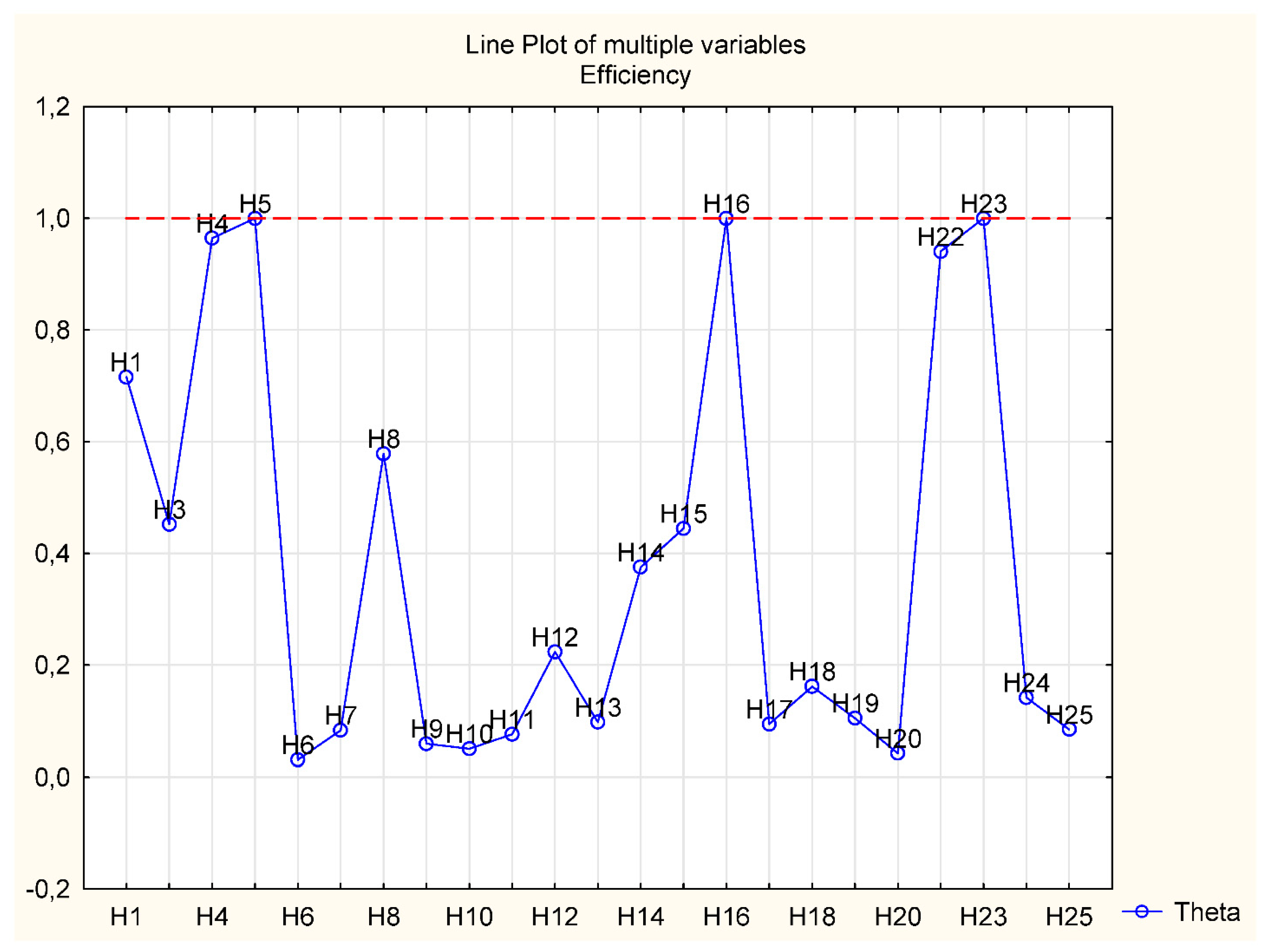
Results of DEA CCR model show that only three hotels achieve efficiency equal to “1” and therefore they are not threatened with bankruptcy. These are hotels H5, H16 and H23.
5. Discussion
Financial results of analyzed hotels are influenced by high internal risks. In particular, risk of lower stocks liquidity on the market, which is given by the amount of equity. Equity does not reach the level required to ensure stability of the hotel. Hotels from the analyzed sample have high indebtedness, which is a prerequisite for the increase of bankruptcy risk. From other internal risks, we can mention business risk. Analyzed hotels are located in the zone of average business risk. Ten hotels from the analyzed sample achieved the highest risk, eight hotels achieved zero risk and seven hotels are located in the zone of average risk. According to Slovak and Czech methodology, Neumaierová and Neumaier (2002), the driver of business risk is ROA. The average value of ROA is around 1%, while median of this indicator achieved negative value. Analyzed hotels achieved the worst results in financial stability risk, the determinant of which is CL. Almost all hotels achieved the highest risk. We can assess this situation as very negative, mainly from the point of view of our research aimed at bankruptcy risk, since insolvency is a prerequisite for it. Capital structure risk achieved average results, similar to business risk. This risk is together with financial stability risk the determinant of business bankruptcy. The assumption of bankruptcy increases when the company fails to cover interest expense with EBIT (Venkataramana et al. 2012).
Based on these results, we can conclude that 22 hotels from the analyzed sample are threatened with bankruptcy, since they do not achieve the required value of CL. Therefore, we can say that these businesses are illiquid. Table 9 shows values of CL as well as values of financial stability risk. Above-mentioned hotels achieved financial stability risk of 10%, which represents the highest possible risk.
Table 6 shows that average ERP of companies doing a business in Slovakia is 5.2%. It does not differ significantly from the ERP of most countries within the EU. Based on the prediction with the use of regression analysis, we can assume that this value will be lower than 5% in 2020. The average CRP of Slovakia is 1.43%. In 2018 it achieved the lowest value 0.98%. Based on the prediction we can assume that the value of country risk premium in 2020 will continue to decline. Coefficient β achieved in the period 2001−2008 values below 1, which means that industry’s yield fluctuated less than the market average in that period. On the other hand, from 2008 to 2015, the value of systematic risk was greater than 1, which means that industry’s yield fluctuated more than the market average. Since 2015, the value of systematic risk has fallen again below 1 and it can be expected that it will drop even more until 2020, which means that external risk in the sector is decreasing.
If we compare the results of overall internal and external risk, we can see that internal risk is much higher than external one. Internal risk is influenced by the results of analyzed hotels and it is a precondition for their bankruptcy. The comparison of overall internal and external risk in percent is shown in Table 10.
The value of external risk is the same for all hotels and considers market risk and country risk. The value of systematic risk is 0.96. Internal risk of analyzed hotels ranges from 5% to the value of maximum possible risk of 35%. Five hotels achieved internal risk of 35%. Only two hotels—H16 and H21—achieved internal risk of 5%, which consists of the risk of lower stocks liquidity on the market. This risk is given by amount of equity. As mentioned above, most hotels face solvency risk. Business risk and capital structure risk of the analyzed sample achieved average values.
Based on DEA model results, we can conclude that three hotels achieved theta equal to “1”. We can say that these hotels are efficient, therefore they are not threatened with bankruptcy. These hotels achieved higher ROA or CL than other hotels, but not at the same time. Two of the analyzed hotels achieved efficiency higher than “0.9”. Therefore, we can assume that these hotels are not threatened with bankruptcy. Two hotels achieved efficiency ranging from “0.5” to “0.9”. Efficiency of other hotels is less than “0.5”, while nine of these hotels achieved value of this indicator less than “0.1”. We can assume that these hotels face higher financial risk and have higher assumption of bankruptcy. The results of DEA model are shown in Figure 3.
Hotels with higher assumption of bankruptcy achieved cost ratio about “1” or higher than “1”. Low efficiency and higher assumption of bankruptcy reported also hotels which achieved negative profitability and low current liquidity. Hotel with cost ratio lower than “1” achieved higher efficiency and lower assumption of bankruptcy. Hotels which reached cost ratio lower than “1” and at the same time low efficiency reported high creditors payment period from 170 days to 834 days.
It should be noted that the results of DEA model are achieved by combining the values of all indicators.
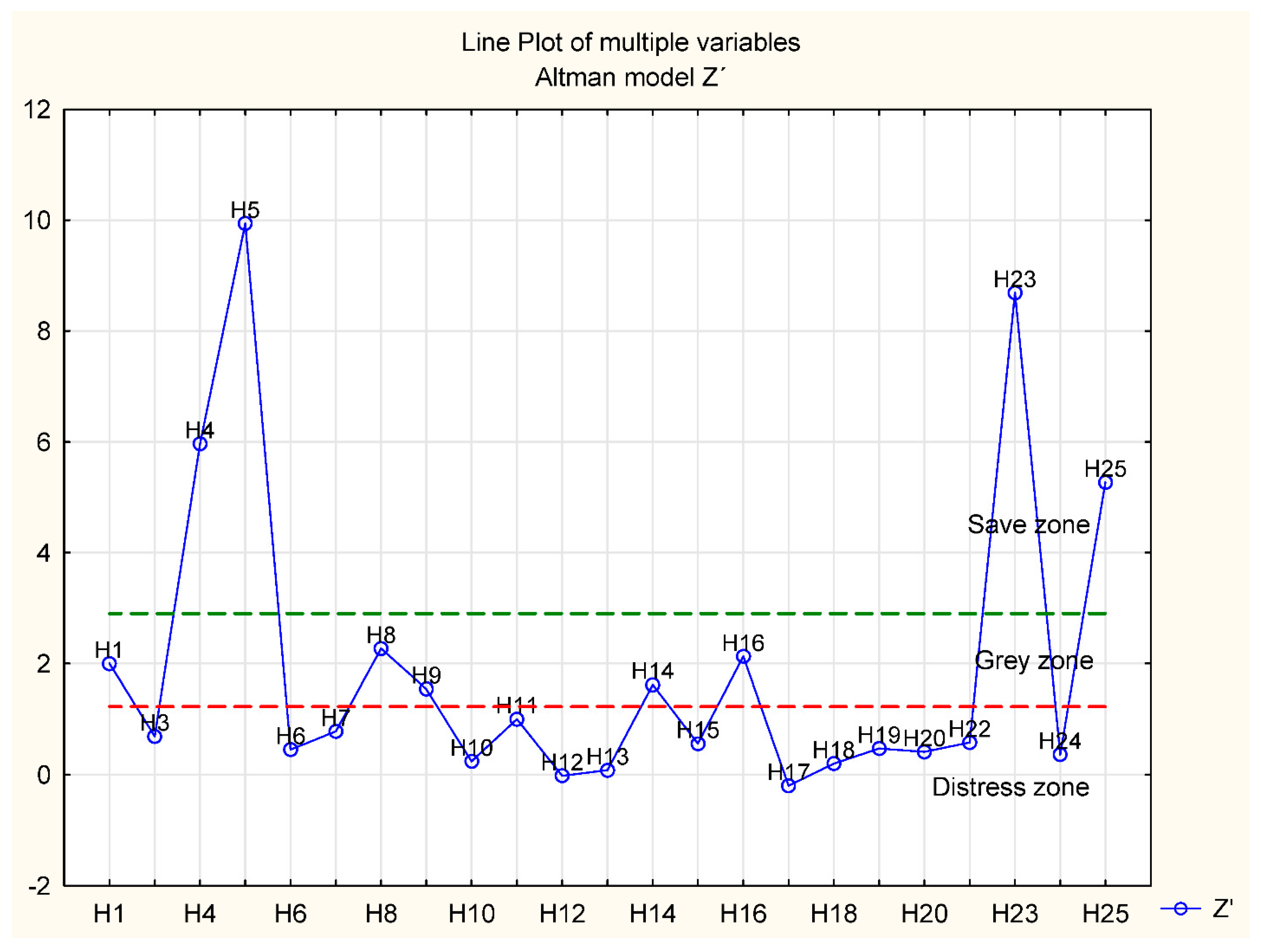
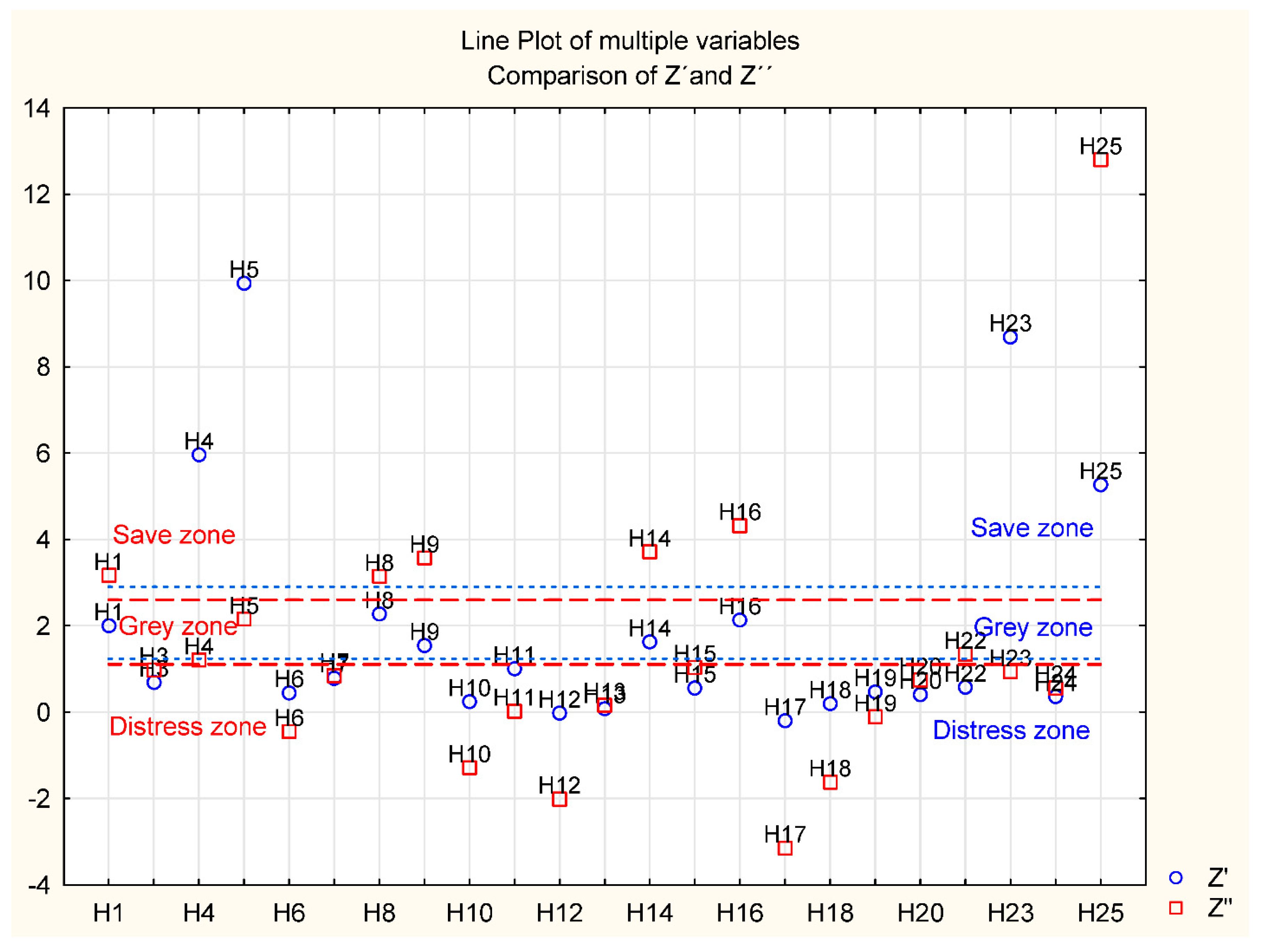
Figure 4 shows that, according to Z’, in safe zone are hotels H4, H5, H23 and H25. Five hotels are in grey zone and remaining hotels are in distress zone. According to Z” (Figure 5), hotels H4, H5 and H23 fell out of safe zone due to the application of the model with only four indicators, except for the indicator x5. Hotels H4 and H5 are located in grey zone and H23 in distress zone. On the other hand, hotel H1 is located in safe zone due to higher values of individual indicators in model. Based on the above-mentioned, we can conclude that only H5 is located in safe zone in both models. Sixteen hotels are located in the distress zone.
If we compare the results of this Altman model with the results associated with financial stability risk, we do not achieve the same results. Therefore, we can conclude that it is appropriate to predict risk of bankruptcy with the use of suitable combination of selected financial indicators. These indicators should represent all areas of business financial health assessment. Very important is the indicator of profitability which represents a production’s strength of the company. This indicator has the highest weight in applied models. We should mention H21 which in terms of financial stability risk did not show assumption of bankruptcy. However, when addressing Altman model, we excluded H21 from the analyzed sample. This hotel achieved negative value of the indicator x4 (book value of equity/book value of total liabilities) and therefore the results were misrepresented. Based on the above-mentioned, we can conclude that, when addressing this issue, considerable attention should be paid to research sample and “clear data” entering the model.
We selected Altman model for the comparison because it is a general model which is most commonly used in Slovak business practice. In addition, we followed the study of Vavřina et al. (2013) who compared the results of DEA with the results of Altman model.
DEA model is not the identical to Altman model. In addition to outputs, it also considers inputs, namely CR and CPP. From this perspective, it is more complex model. Therefore, the results of both models are not entirely the same. According to DEA model, hotels H5, H16 and H23 are financially healthy and are not threatened with bankruptcy. These hotels show good results also in Altman model. H1 achieved in DEA model efficiency 0.72. We can assume that this hotel is in grey zone and it is due to values of liquidity and cost ratio. H25, which according to Altman model is in safe zone, is located in distressed zone according to DEA model. It was caused by cost ratio 1.49. Therefore, it is necessary to point out these facts: careful selection of indicators which are used in models is necessary, and not only outputs but also inputs should be selected to ensure complexity of the model. Cost ratio is one of the most important indicators applied by Slovak companies. The value of this indicator above “1” causes bankruptcy and it is equally significant as liquidity and profitability indicators. Based on the above-mentioned, we can conclude that DEA fills the gap in the prediction of bankruptcy in terms of the application of operational indicators, i.e., inputs.
DEA method has been used in many empirical studies. Many researchers combined DEA method with other conventional techniques. Xu and Wang (2009) applied conventional DEA approach and used DEA score as a predictor in conventional techniques—discriminant analysis (DA), linear regression (LR)—as well as mechanism of supporting vectors. They concluded that the inclusion of DEA score in these models decreased the rate of misclassification. Ferus (2010) applied conventional DEA approach and approximated DEA score using linear regression. He found that the proposed DEA approach achieved comparable classification accuracy to traditional techniques (DA and LR). Araghi and Makvandi (2013) used not only conventional DEA but also inverse DEA as predictors in LR. They quantified 72% overall accuracy of DEA, which is less compared to LR. Premachandra et al. (2011) combined conventional DEA and negative DEA and created DEA evaluation index. This index correctly classified 84% of businesses threatened with bankruptcy. However, the rate of classification of financially healthy businesses was relatively low. Nevertheless, these authors argued that, compared to other statistical methods, DEA has unique features making it an excellent tool for predicting bankruptcy.
Some authors compared the results of DEA method with the results of other conventional techniques. Mendelová and Bieliková (2017) compared the results of negative DEA, logistic regression and decision trees. Since DEA is highly sensitive to extremes and outliers, they proposed two-step procedure to eliminate them. The study assessed the classification ability of DEA model at the level of 78.5%, classification ability of other methods was more than 90%. Moreover, Mendelová and Bieliková concluded that the application of proposed two-step procedure to DEA method shows relatively satisfactory results in terms of correct classification of non-bankrupt businesses. Vavřina et al. (2013) compared the results of DEA method, LR and Altman Z-score. Overall probability of correct classification of DEA model overcame other approaches. Therefore, they concluded that DEA appears to be superior to Altman Z-score and LR when evaluating a dataset with few businesses threatened with bankruptcy.
Based on the comparison of the results of DEA model and Altman model, this paper reveals that classification ability of DEA model is 78.5%. This result is approximately the same as the results of above-mentioned studies. To achieve this, we ranked hotels according to Altman model and DEA model (Table 11).
6. Conclusions
Slovak government promotes tourism in its program statements. Their aim is to keep existing hotel facilities at the required level in terms of quantity but especially quality. It requires extensive cooperation of hotel facilities. Awareness of current state and indication of their possible bankruptcy can be beneficial in terms of strengthening Slovak economy.
In this context, DEA model seems to be an appropriate tool to diagnose bankruptcy. Compared to statistical and other methods, DEA is relatively new non-parametric method. It represents one of the methods which can be applied when determining the risk of bankruptcy. This method also allows us to evaluate individual production units with respect to whole sample. The benefit of this method is to find out how to increase or decrease inputs or outputs to achieve financial health. The most significant benefit of this method is identifying a “peer unit” for an inefficient businesses. This peer unit is an efficient unit which represents efficient consumption of inputs and production of outputs for an inefficient unit. Important advantage of DEA is the possibility to predict financial health of businesses. When addressing DEA model we can apply user-friendly software solution, which is also the great benefit. The disadvantage of DEA method is a deterministic approach—we directly assume the type of returns (constant returns to scale model and variable returns to scale model). The statistical testing of the significance of various inputs and outputs within this method is not processed at the same level as for example in econometric analysis yet. However, it is an area in which we can expect next development, which will definitely lead to improvement of this approach.
The limitations of the study come from the availability of the data in Slovak register of financial statements. We obtained complete data for only 25 hotels. Therefore, in our further research, we will focus on gaining larger amount of data. In addition to the data quantity, we also had problems with data quality. It was necessary to exclude some hotels from the analyzed sample. Equity of these hotels was negative and they achieved high value of interest coverage. These values degenerated results of DEA. Our research shows that in future it will be necessary to work on the classification accuracy of DEA in the diagnosis of bankruptcy. It will also be appropriate to compare the results of DEA model with the results of LR. According to the study of Premachandra et al. (2011), later followed by Araghi and Makvandi (2013), when comparing the results of DEA model, we apply model LR.
Despite all objections to DEA model, it is a great tool for business bankruptcy prediction (Premachandra et al. 2011).
Author Contributions
All authors contributed equally of this work.
Funding
This research was carried out within the Slovak grant scheme VEGA.
Acknowledgments
This paper was prepared within the grant scheme VEGA No. 1/0887/17 (Increasing the competitiveness of Slovakia within the EU by improving efficiency and performance of production systems) and the grant scheme VEGA No. 1/0791/16 (Modern approaches to improving enterprise performance and competitiveness using the innovative model—Enterprise Performance Model to streamline Management Decision-Making Processes).
Conflicts of Interest
The authors declare no conflict of interest.
References
- Adamko, Peter, and Lucia Svabova. 2016. Prediction of the risk of bankruptcy of Slovak companies. Paper present at 8th International Scientific Conference Managing and Modelling of Financial Risks, Ostrava, Czech Republic, 5–6 September 2016; pp. 15–20. Available online: https://www.ekf.vsb.cz/export/sites/ekf/rmfr/cs/sbornik/Soubory/Part_I.pdf (accessed on 1 August 2018).
- Agarwal, Vineet, and Richard Taffler. 2008. Comparing the performance of market-based and accounting-based bankruptcy prediction models. Journal of Banking & Finance 32: 1541–51. [Google Scholar] [CrossRef] [Green Version]
- Albright, Jeremy. 2015. What Is the Difference between Logit and Probit Model? Available online: https://www.methodsconsultants.com/tutorial/what-is-the-difference-between-logit-and-probit-models/ (accessed on 10 July 2018).
- Aleksanyan, Lilia, and Jean-Pierre Huiban. 2016. Economic and Financial Determinants of Firm Bankruptcy: Evidence from the French Food Industry. Review of Agricultural, Food and Environmental Studies 97: 89–108. [Google Scholar] [CrossRef]
- Altman, Edward I., Malgorzata Iwanicz-Drozdowska, Erkki K. Laitinen, and Arto Suvas. 2014. Distressed Firm and Bankruptcy Prediction in an International Context: A Review and Empirical Analysis of Altman’s Z-score Model. Available online: https://papers.ssrn.com/sol3/papers.cfm?abstract_id=2536340 (accessed on 20 July 2018).
- Altman, Edward I. 1982. Accounting Implications of Failure Prediction Models. Journal of Accounting Auditing and Finance 6: 4–19. [Google Scholar]
- Araghi, Maryam K., and Sara Makvandi. 2013. Comparing Logit, Probit and Multiple Discriminant Analysis Models in Predicting Bankruptcy of Companies. Asian Journal of Finance & Accounting 5: 48–59. [Google Scholar] [CrossRef]
- Aziz, Adnan A., and Humayon A. Dar. 2006. Predicting corporate bankruptcy: where we stand? Corporate Governance 6: 18–33. [Google Scholar] [CrossRef]
- Banker, Rajiv. D., Abraham Charnes, and William. W. Cooper. 1984. Some Models for Estimating Technical Scale Inefficiencies in Data Envelopment Analysis. Management Science 30: 1078–92. [Google Scholar] [CrossRef]
- Bauer, Julian, and Vineet Agarwal. 2014. Are hazard models superior to traditional bankruptcy prediction approaches? A comprehensive test. Journal of Banking & Finance 40: 432–42. [Google Scholar] [CrossRef]
- Beaver, William H. 1966. Financial ratios as predictors of failure. Journal of Accounting Research 4: 71–111. [Google Scholar] [CrossRef]
- Becchetti, Leonardo, and Jaime Sierra. 2002. Bankruptcy risk and productive efficiency in manufacturing firms. Journal of Banking and Finance 27: 2099–20. [Google Scholar] [CrossRef]
- Black, Fischer, and Myron Scholes. 1973. The pricing of options and corporate liabilities. Journal of Political Economy 81: 637–54. [Google Scholar] [CrossRef]
- Blum, Marc. 1974. Failing Company Discriminant Analysis. Journal of Accounting Research 12: 1–25. [Google Scholar] [CrossRef]
- Booth, Peter J. 1983. Decomposition measure and the prediction of financial failure. Journal of Business Finance & Accounting 10: 67–82. [Google Scholar] [CrossRef]
- Buganová, Katarína, and Mária Hudáková. 2012. Manažment rizika v podniku, 1st ed. Žiline: EDIS, ISBN 978-80554-0459-2. [Google Scholar]
- Campbell, Harvey R. 2012. Bankruptcy Risk. Available online: https://financial-dictionary.thefreedictionary.com/Bankruptcy + risk (accessed on 15 July 2018).
- Charnes, Abraham, William W. Cooper, and Jean E. Rhodes. 1978. Measuring the Efficiency of Decision Making Units. European Journal of Operational Research 2: 429–44. [Google Scholar] [CrossRef]
- Chen, Ning, Bernardete Ribeiro, Armando Vieira, and An Chen. 2013. Clustering and visualization of bankruptcy trajectory using self−organizing map. Expert Systems with Applications 40: 385–93. [Google Scholar] [CrossRef]
- Chrastinová, Zuzana. 1998. Metódy Hodnotenia Ekonomickej Bonity a Predickei Finančnej situácie Poľnohospodárskych Podnikov. Bratislava: VÚEPP, ISBN 80-8058-022-7. [Google Scholar]
- Cisko, Štefan, and Tomáš Klieštik. 2013. Finančný manažment podniku II. Žilina: EDIS, ISBN 978-80-554-0684-8. [Google Scholar]
- Cornuejols, Gerard, and Michael Trick. 1998. Quantitative Methods for the Management Sciences. Pittsburgh: Carnegie Mellon University, Available online: http://mat.gsia.cmu.edu/classes/QUANT/NOTES/chap0.pdf (accessed on 11 May 2018).
- Čunderlík, Dušan. 2004. Rizikový manažment a riadenie kontinuity podnikateľskej činnosti podniku. Available online: http://fsi.uniza.sk/kkm/old/publikacie/pp/pp_kap_12.pdf (accessed on 12 August 2018).
- Damodaran, Aswath. 2018. The Data Page. Available online: http://pages.stern.nyu.edu/adamodar/ (accessed on 12 July 2018).
- Damodaran, Aswath. 2014. Equity Risk Premiums: Looking Backwards and Towards. Available online: http://people.stern.nyu.edu/adamodar/pdfiles/country/ERP2014.pdf (accessed on 14 May 2018).
- Das, Sanjiv R., Paul Hanouna, and Atulya Sarin. 2009. Accounting−Based versus Market−Based cross-sectional models for CDS spreads. Journal of Banking & Finance 33: 719–30. [Google Scholar] [CrossRef]
- Deakin, Edward B. 1972. A Discriminant Analysis of Predictors of Business Failure. Journal of Accounting Research 10: 167–79. [Google Scholar] [CrossRef]
- Farrell, Michael J. 1957. The Measurement of Productive Efficiency. Journal of the Royal Statistical Society, Series A 120: 253–90. [Google Scholar] [CrossRef]
- Ferus, Anna. 2010. The Application of DEA Method in Evaluating Credit Risk of Companies. Contemporary Economics 4: 107–13. [Google Scholar]
- Fetisovová, Elena, Karol Vlachynský, and Vladimír Sirotka. 2004. Financie malých a stredných podnikov, 1st ed. Bratislava: Iura Edition, ISBN 80-89047-87-4. [Google Scholar]
- Fulmer, John. G., Jr., James. E. Moon, Thomas. A. Gavin, and Michael. J. Erwin. 2004. A bankruptcy classification model for small firms. Journal of Commercial Bank Iandirg 66: 25–37. [Google Scholar]
- Friedman, Jerome H. 1977. A recursive partitioning decision rule for nonparametric classification. IEEE Transactions on Computers 26: 404–8. [Google Scholar] [CrossRef]
- Gherghina, Stefan C. 2015. An Artificial Intelligence Approach towards Investigating Corporate Bankruptcy. Review of European Studies 7: 5–22. [Google Scholar] [CrossRef]
- Gurčík, Ľubomír. 2002. G—index—metóda predikcie finančního stavu poľnohospodárskych podnikov. Agricultural Economics 48: 373–8. [Google Scholar]
- Gurney, Kevin. 1997. An Introduction to Neural Networks. London: UCL Press Limited, ISBN 0-203-45151-1. Available online: https://www.inf.ed.ac.uk/teaching/courses/nlu/assets/reading/Gurney_et_al.pdf (accessed on 24 August 2018).
- Horváthová, Jarmila, and Martina Mokrišová. 2018. The use of innovative approaches in assessing and predicting business financial health. Paper presented at 27th International Scientific Conference on Economic and Social Development, Rome, Italy, March 1–2; pp. 728–38. Available online: http://www.esd-conference.com/past-conferences (accessed on 12 March 2018).
- Karels, Gordon V., and Arun J. Prakash. 1987. Multivariate Normality and Forecasting of Business Bankruptcy. Journal of Business Finance & Accounting 14: 573–93. [Google Scholar] [CrossRef]
- Kidane, Habtom W. 2004. Predicting Financial Distress in IT and Services Companies in South Africa. Master’s thesis, Faculty of Economics and Management Sciences, Bloemfontein, South Africa. Available online: http://scholar.ufs.ac.za:8080/xmlui/handle/11660/1117 (accessed on 18 June 2018).
- Klieštik, Tomáš, Jana Majerová, and Alexander N. Lyakin. 2015. Metamorphoses and Semantics of Corporate Failures as a Basal Assumption of a Well−founded Prediction of a Corporate Financial Health. Paper presented at 3rd International Conference on Economics and Social Science (ICESS 2015), Changsha, China, December 28–29; vol. 86, pp. 150–4. [Google Scholar]
- Klučka, Jozef. 2006. Riadenie rizika a hodnotenie výkonnosti podniku. BIATEC 14: 22–25. [Google Scholar]
- Koscielniak, Helena. 2014. An improvement of information processes in enterprises—The analysis of sales profitability in the manufacturing company using ERP systems. Polish Journal of Management Studies 10: 65–71. [Google Scholar]
- Kürschner, Manuel. 2008. Limitation of the Capital Asset Princing Model (CAPM). Munich: GRIN Verlag, ISBN 978-3-640-09925. [Google Scholar]
- Lippmann, Richard P. 1987. An Introduction to Computing with Neural Nets. IEEE ASSP Magazine 4: 4–22. [Google Scholar] [CrossRef]
- Liu, Li-lin, Kathryn J. Jervis, Mustafa Z. Younis, and Dana A. Forgione. 2011. Hospital financial distress, recovery and closure: Managerial incentives and political costs. Journal of Public Budgeting, Accounting and Financial Management 23: 31–68. [Google Scholar] [CrossRef]
- Lowrance, William. W. 1976. Of Acceptable Risk. Los Altos: William Kaufman Inc. [Google Scholar]
- Lukason, Oliver, and Erkki K. Laitinen. 2018. Firm failure processes and components of failure risk: An analysis of European bankrupt firms. Journal of Business Research. [Google Scholar] [CrossRef]
- Maddala, Gangadharrao S. 1983. Limited Dependent and Qualitative Variables in Econometrics. Cambridge: Cambridge University Press. [Google Scholar] [CrossRef]
- Mařík, Miloš, Karel Čada, Pavla Maříková, Barbora Rýdlová, and Josef Rajdl. 2011. Metody Oceňování Podniku: Proces Ocenění—Základní metody a Postupy, 3rd ed. Praha: Ekopress, ISBN 978-80-86929-67-5. [Google Scholar]
- Marinič, Pavel. 2008. Plánovaní a Tvorba Hodnoty Firmy. Praha: Grada Publishing, a. s., ISBN 978-80-247-2432-4. [Google Scholar]
- Markovič, Peter. 2010. Opcia a investičný projekt. Finančný Manažment a Controlling 2010: 627–30. [Google Scholar]
- Mendelová, Viera, and Tatiana Bieliková. 2017. Diagnostikovanie finančného zdravia podnikov pomocou metódy DEA: aplikácia na podniky v Slovenskej republike. Politická ekonomie 65: 26–44. [Google Scholar] [CrossRef]
- Min, Hokey, Hyesung Min, Seong J. Joo, and Joungman Kim. 2008. A Data Envelopment Analysis for establishing the financial benchmark of Korean hotels. International Journal of Services and Operations Management 4: 201–17. [Google Scholar] [CrossRef]
- Misankova, Maria, and Viera Bartosova. 2016. Comparison of selected statistical methods for the prediction of bankruptcy. Paper presented at 10th International Days of Statistics and Economics, Prague, Czech Republic, September 8–10; pp. 1260–69. Available online: https://msed.vse.cz/msed_2016/article/205-Misankova-Maria-paper.pdf (accessed on 20 August 2018).
- Mokrišová, Martina, and Jarmila Horváthová. 2018. Linear model as a tool in the process of improving financial health. Paper presented at 28th International Scientific Conference on Economic and Social Development, Paris, France, April 19–20; pp. 435–44. Available online: http://www.esd-conference.com/past-conferences (accessed on 22 May 2018).
- Moyer, Charles R. 1977. Forecasting Financial Failure: A Reexamination. Financial Management 6: 11–7. [Google Scholar] [CrossRef]
- Neumaierová, Inka, and Ivan Neumaier. 2002. Výkonnost a tržní hodnota firmy. Praha: Grada Publishing, ISBN 80-247-0125-1. [Google Scholar]
- Odom, Marcus D., and Ramesh Sharda. 1990. A neural Network Model for Bankruptcy Prediction. Paper presented at International Joint Conference on Neural Networks, San Diego, CA, USA, June 17–21. [Google Scholar] [CrossRef]
- Ohlson, James A. 1980. Financial Ratios and the Probabilistic Prediction of Bankruptcy. Journal of Accounting Research 18: 109–31. [Google Scholar] [CrossRef]
- Premachandra, I. M., Yao Chen, and John Watson. 2011. DEA as a Tool for Predicting Corporate Failure and Success: A Case of Bankruptcy Assessment. Omega 39: 620–6. [Google Scholar] [CrossRef]
- Rahimian, E., S. Singh, T. Thammachote, and R. Virmani. 1993. Bankruptcy prediction by neural network. In Neural Networks in Finance and Investing: Using Artificial Intelligence to Improve Real−World Performance. Edited by Robert R. Trippi and Efraim Turban. Chicago: Probus, pp. 159–76. [Google Scholar]
- Reisz, Alexander S., and Claudia Perlich. 2007. A market-based framework for bankruptcy prediction. Journal of Financial Stability 3: 85–131. [Google Scholar] [CrossRef]
- RÚZ. 2018. Register účtovných závierok. Available online: http://www.registeruz.sk/cruz-public/home/ (accessed on 20 August 2018).
- Rybak, Tatsiana R. 2006. Analysis and estimate of the enterprises bankruptcy risk. Paper presented at the 3rd International Conference Řízení a Modelování Finančních Rizik, Ostrava, Czech Republic, September 6–7; pp. 315–20. [Google Scholar]
- Salchenberger, Linda M., E. Mine Cinar, and Nicholas A. Lash. 1992. Neural networks: A new tool for predicting thrift failures. Decision Sciences 23: 899–916. [Google Scholar] [CrossRef]
- Scott, James. 1981. The probability of bankruptcy: A comparison of empirical predictions and theoretical models. Journal of Banking & Finance 5: 317–44. [Google Scholar] [CrossRef]
- Siegel, Jeffrey G. 1981. Warning Signs of Impending Business Failure and Means to Counteract such Prospective Failure. The National Public Accountant 24: 9–13. [Google Scholar]
- Simak, Paul C. 2000. Inverse and Negative DEA and Their Application to Credit Risk Evaluation. Ph.D. dissertation, University of Toronto, ON, Canada. Available online: https://tspace.library.utoronto.ca/bitstream/1807/13948/1/NQ49942.pdf (accessed on 20 August 2018).
- Soon, Ng Kim, Absulah A. Mohammed, and Rahil M. Mostafa. 2014. Using Altman’s Z−Score Model to Predict the Financial Hardship of Companies Listed in the Trading Services Sector of Malaysian Stock Exchange. Australian Journal of Basic and Applied Sciences 8: 379–84. [Google Scholar]
- Springate, Gordon L. V. 1978. Predicting the possibility of failure in a Canadian firm: A discriminant analysis. Unpublished M.B.A. Research Project, Simon Eraser University. [Google Scholar]
- Spuchľáková, Erika, and Katarína Frajtová-Michalíková. 2016. Comparison of LOGIT, PROBIT and neural network bankruptcy prediction models. Paper presented at ISSGBM International Conference on Information and Business Management, Hong Kong, China, September 3–4; pp. 49–53, ISBN 978-981-09-9757-1. [Google Scholar]
- Sulub, Saed A. 2014. Testing the Predictive Power of Altman’s Revised Z’ Model: The Case of 10 Multinational Companies. Research Journal of Finance and Accounting 5: 174–184. [Google Scholar]
- Šarlija, Nataša, and Marina Jeger. 2011. Comparing financial distress prediction models before and during recession. Croatian Operational Research Review 2: 133–42. [Google Scholar]
- Šotić, Aleksander, and Radenko Rajić. 2015. The review of the definition of risk. Journal of Apllied Knowledge Management 3: 17–26. [Google Scholar]
- Taffler, Richard J. 1984. Empirical Models for the Monitoring of UK Corporations. Journal of Banking & Finance 8: 199–227. [Google Scholar] [CrossRef]
- Tej, Juraj, František Bartko, and Viktória Ali Taha. 2013. Manažment rizík a zmien, 1st ed. Prešov: Bookman, ISBN 978-80-89568-73-4. [Google Scholar]
- Tranchard, Sandrine. 2018. The new ISO 31000 Keeps Risk Management Simple. Available online: https://www.iso.org/news/ref2263.html (accessed on 29 August 2018).
- Valášková, Katarína, Lucia Švábová, and Marek Ďurica. 2017. Verifikácia predikčných modelov v podmienkach slovenského poľnohospodárskeho sektora. Ekonomika Management Inovace 9: 30–38. [Google Scholar]
- Vavřina, Jan, David Hampel, and Jitka Janová. 2013. New Approaches for the Financial Distress Classification in Agribusiness. Acta Universitatis Agriculturae et Silviculturae Mendelianae Brunensis 61: 1177–82. [Google Scholar] [CrossRef]
- Venkataramana, N., Md. Azash, and K. Ramakrishnaiah. 2012. Financial Performance and Predicting the Risk of Bankruptcy: A Case of Selected Cement Companies in India. International Journal of Public Administration and Management Research 1: 40–56. [Google Scholar]
- Xu, Xiaoyan, and Yu Wang. 2009. Financial Failure Prediction Using Efficiency as a Predictor. Expert Systems with Applications 36: 366–73. [Google Scholar] [CrossRef]
- Závarská, Zuzana. 2012. Manažment kapitálovej štruktúry pri financovaní rozvoja podniku ako nástroj zvyšovania finančnej výkonnosti. Prešov: Prešovská univerzita, ISBN 978-80-555-0553-4. [Google Scholar]
- Zmijewski, Mark E. 1984. Methodological Issues Related to the Estimation of Financial Distress Prediction Models. Journal of Accounting Research 22: 59–82. [Google Scholar] [CrossRef]
Figure 1.
Flowchart of the research.

Figure 2.
The example of inserting objective function and conditions in Solver.

Figure 3.
Results of efficiency.

Figure 4.
Results of Z’.

Figure 5.
The comparison of Z’ and Z”.


Table 1.
Method used to compute selected financial indicators.
| Indicator | Computation method | |
|---|---|---|
| CL | current liquidity | |
| TL | total liquidity | |
| TATR | total assets turnover ratio | |
| ACP | average collection period | |
| CPP | creditors payment period | |
| IR | indebtedness ratio | |
| ER | equity ratio | |
| IC | interest coverage | |
| ROE | return on equity | |
| ROS | return on sales | |
| ROA | return on assets | |
| CR | cost ratio | |
Table 2.
Conditions for hotel internal risks assessment.
| Risk Premium | Values | Criteria |
|---|---|---|
| rSL | E – equity | |
| rbusiness | EBIT − earnings before interest and taxes I – interests D − debt A – assets | |
X − average return on assets of businesses in given industry | ||
| rfinstab | CR − current ratio XL − average current ratio of businesses in given industry | |
| rcapstr | ||
Table 3.
The example of data processing in Solver.
| Hotels | CR | CPP | CL | ROA | SS | L1 | L3 | L4 | L5 | … | ϴ | Min z= 0 | C1 <= 0 | … | C5 >= 0.6 |
|---|---|---|---|---|---|---|---|---|---|---|---|---|---|---|---|
| H1 | 0.96 | 0.19 | 0.6 | 0.04 | 0.62 | 0 | 0 | 0 | 0.05 | 0.71 | 0.71 | −0.07 | … | 0.6 | |
| H3 | 0.91 | 0.54 | 0.1 | 0.03 | 0.45 | 0 | 0 | 0 | 0.07 | 0.45 | 0.45 | −0.29 | … | 0.1 | |
| H4 | 1 | 0.16 | 1 | 0.02 | 0.05 | 0 | 0 | 0 | 0 | 0.96 | 0.96 | 0 | … | 0.97 | |
| H5 | 0.95 | 0.09 | 0.77 | 0.39 | 0.16 | 0 | 0 | 0 | 1 | 1 | 1 | 0 | … | … | |
| H6 | 1.008 | 2.66 | 0.03 | 0.01 | 0.43 | 0 | 0 | 0 | 0.02 | 0.03 | 0.03 | 0 | … | … | |
| H7 | 0.94 | 0.47 | 0.04 | 0.03 | 0.54 | 0 | 0 | 0 | 0.08 | 0.08 | 0.08 | 0 | … | … | |
| H8 | 0.97 | 0.17 | 0.8 | 0.08 | 0.71 | 0 | 0 | 0 | 0.15 | 0.57 | 0.57 | 0 | … | … | |
| … | … | … | … | … | … | … | … | … | … | … | … | … | … | … | … |
| … | … | ||||||||||||||
| … | … | … | … | … | … | … | … | … | … | … | … | … | … | … | … |
| H25 | 1.39 | 0.53 | 0.19 | −0.06 | 0.92 | 0 | 0 | 0 | 0 | ……… | 0.08 | 0.08 | 0 | … | … |
Table 4.
Descriptive statistics for selected financial indicators.
| Variable | Valid N | Mean | Median | Minimum | Maximum | Std. Dev. |
|---|---|---|---|---|---|---|
| CL | 25 | 0.404 | 0.16 | 0 | 1.45 | 0.44 |
| TL | 25 | 0.482 | 0.20 | 0 | 1.6 | 0.49 |
| TATR | 25 | 1.58 | 0.26 | 0 | 8.74 | 2.76 |
| ACP | 25 | 0.10 | 0.04 | 0 | 0.65 | 0.16 |
| CPP | 25 | 1.20 | 0.55 | 0.1 | 7.53 | 1.64 |
| IR | 25 | 0.71 | 0.71 | 0.1 | 1.87 | 0.4 |
| ER | 25 | 0.29 | 0.28 | −0.9 | 0.93 | 0.4 |
| IC | 25 | −871.47 | 1.19 | −47,337.7 | 25,388.0 | 10,928.71 |
| ROE | 25 | 0.11 | 0.01 | −0.7 | 1.78 | 0.55 |
| ROS | 25 | −0.069 | 0.004 | −0.7 | 0.07 | 0.18 |
| ROA | 25 | −0.029 | 0.014 | −1.5 | 0.39 | 0.32 |
| CR | 25 | 1.059 | 0.99 | 0.9 | 1.5 | 0.16 |
Table 5.
Results of selected internal risks.
| Indicator | H1 | H2 | H3 | H4 | H5 | H6 | H7 | H8 | H9 |
| E(€) | 1,518,354 | −409,612 | 4,577,340 | 63,874 | 14,194 | 1,597,188 | 907,038 | 2,039,044 | 11,248,789 |
| rSL (%) | 5.00 | 5.00 | 4.87 | 5.00 | 5.00 | 5.00 | 5.00 | 5.00 | 4.21 |
| ROA | 0.04 | −1.52 | 0.03 | 0.02 | 0.39 | 0.01 | 0.03 | 0.08 | −0.03 |
| rbusiness (%) | 0.05 | 10.00 | 3.04 | 0.00 | 0.00 | 4.45 | 0.00 | 0.00 | 10.00 |
| CL | 0.46 | 0.41 | 0.06 | 0.85 | 0.65 | 0.02 | 0.05 | 0.69 | 0.09 |
| rfinstab (%) | 10.00 | 10.00 | 10.00 | 10.00 | 10.00 | 10.00 | 10.00 | 10.00 | 10.00 |
| IC | 8.30 | −72.05 | 3.75 | 25,388.00 | 219.37 | 0.87 | 1.78 | 1.60 | −44.51 |
| rcapstr (%) | 0.00 | 10.00 | 0.00 | 0.00 | 0.00 | 10.00 | 3.70 | 4.93 | 10.00 |
| Indicator | H10 | H11 | H12 | H13 | H14 | H15 | H16 | H17 | H18 |
| E(€) | 239,330 | 5,605,784 | 2,429,811 | 1,621,510 | 22,000,368 | 7,291,295 | 2,844,134 | 598,602 | 544,180 |
| rSL (%) | 5.00 | 4.77 | 5.00 | 5.00 | 3.25 | 4.60 | 5.00 | 5.00 | 5.00 |
| ROA | 0.02 | 0.01 | −0.06 | −0.03 | 0.00 | 0.01 | 0.05 | 0.00 | −0.06 |
| rbusiness (%) | 0.00 | 9.51 | 10.00 | 10.00 | 10.00 | 4.56 | 0.00 | 10.00 | 10.00 |
| CL | 0.04 | 0.07 | 0.17 | 0.11 | 0.61 | 0.54 | 1.39 | 0.10 | 0.16 |
| rfinstab (%) | 10.00 | 10.00 | 10.00 | 10.00 | 10.00 | 10.00 | 0.00 | 10.00 | 10.00 |
| IC | 2.66 | 1.19 | −3.62 | −2.03 | −0.71 | 2.53 | 51.03 | −0.15 | −14.23 |
| rcapstr (%) | 0.29 | 8.19 | 10.00 | 10.00 | 10.00 | 0.55 | 0.00 | 10.00 | 10.00 |
| Indicator | H19 | H20 | H21 | H22 | H23 | H24 | H25 | ||
| E(€) | 874,218 | 2,266,362 | −291,054 | 638,301 | 21,678 | 732,519 | 7,814,753 | ||
| rSL (%) | 5.00 | 5.00 | 5.00 | 5.00 | 5.00 | 5.00 | 4.54 | ||
| ROA | 0.01 | 0.00 | 0.23 | 0.00 | 0.05 | 0.03 | −0.06 | ||
| rbusiness (%) | 4.78 | 10.00 | 0.00 | 10.00 | 0.00 | 1.98 | 10.00 | ||
| CL | 0.10 | 0.05 | 1.45 | 1.19 | 0.70 | 0.08 | 0.07 | ||
| rfinstab (%) | 10.00 | 10.00 | 0.00 | 0.03 | 10.00 | 10.00 | 10.00 | ||
| IC | 0.00 | 1.27 | 4.00 | 0.03 | 0.00 | 1.91 | −47,337.70 | ||
| rcapstr (%) | 10.00 | 7.48 | 0.00 | 10.00 | 10.00 | 2.99 | 10.00 |
Table 6.
The development and prediction of external risks.
| Year | ERP % | CRP % | B |
|---|---|---|---|
| 2001 | 5.51 | 2.5 | 0.84 |
| 2002 | 5.51 | 1.45 | 0.9 |
| 2003 | 4.51 | 2.03 | 0.91 |
| 2004 | 4.82 | 1.43 | 0.84 |
| 2005 | 4.84 | 1.43 | 0.74 |
| 2006 | 4.8 | 1.2 | 0.82 |
| 2007 | 4.91 | 1.05 | 0.77 |
| 2008 | 4.79 | 1.05 | 1.25 |
| 2009 | 5 | 2.1 | 1.7 |
| 2010 | 4.5 | 1.35 | 1.74 |
| 2011 | 5 | 1.28 | 1.75 |
| 2012 | 6 | 1.28 | 1.74 |
| 2013 | 5.8 | 1.5 | 1.65 |
| 2014 | 5 | 1.28 | 1.27 |
| 2015 | 5.75 | 1.28 | 1.18 |
| 2016 | 6.25 | 1.33 | 0.97 |
| 2017 | 5.69 | 1.21 | 0.96 |
| 2018 | 5.08 | 0.98 | 0.94 |
| 2019 | 5.08 | 0.69 | 0.81 |
| 2020 | 4.66 | 0.34 | 0.65 |
Source: Processed by authors based on Damodaran’s data.
Table 7.
Results of Altman model.
| H1 | H2 | H3 | H4 | H5 | H6 | H7 | H8 | H9 | H10 | H11 | H12 | H13 | |
| Z’ | 2.00 | 1.87 | 0.69 | 5.96 | 9.94 | 0.45 | 0.78 | 2.27 | 1.54 | 0.24 | 1.00 | −0.02 | 0.08 |
| Z’’ | 3.16 | −15.23 | 0.97 | 1.20 | 2.15 | −0.45 | 0.84 | 3.14 | 3.57 | −1.29 | 0.02 | −2.01 | 0.16 |
| H14 | H15 | H16 | H17 | H18 | H19 | H20 | H21 | H22 | H23 | H24 | H25 | ||
| Z’ | 1.62 | 0.56 | 2.13 | −0.20 | 0.20 | 0.47 | 0.41 | 3.41 | 0.58 | 8.69 | 0.36 | 5.27 | |
| Z” | 3.71 | 1.03 | 4.32 | −3.14 | −1.62 | −0.11 | 0.74 | 3.18 | 1.33 | 0.93 | 0.56 | 12.80 |
Table 8.
Results of DEA model.
| CR | CPP | CL | ROA | ER | ϴ | |
|---|---|---|---|---|---|---|
| H1 | 0.9579 | 0.196655 | 0.6 | 0.0441 | 0.6188 | 0.715571 |
| H3 | 0.9124 | 0.546228 | 0.1 | 0.0319 | 0.445 | 0.452083 |
| H4 | 0.9965 | 0.163558 | 0.97 | 0.0202 | 0.0509 | 0.964491 |
| H5 | 0.9569 | 0.095564 | 0.77 | 0.3894 | 0.1647 | 1 |
| H6 | 1.0083 | 2.669453 | 0.03 | 0.0108 | 0.4639 | 0.031132 |
| H7 | 0.9409 | 0.471121 | 0.04 | 0.0321 | 0.5425 | 0.083836 |
| H8 | 0.9688 | 0.173098 | 0.8 | 0.0829 | 0.7143 | 0.578691 |
| H9 | 1.138 | 1.334135 | 0.1128 | −0.025 | 0.7712 | 0.059882 |
| H10 | 0.967 | 2.317649 | 0.0429 | 0.0156 | 0.1511 | 0.050876 |
| H11 | 0.9888 | 0.625902 | 0.0994 | 0.0149 | 0.6047 | 0.076718 |
| H12 | 1.3649 | 2.879761 | 0.3632 | −0.0574 | 0.2881 | 0.223671 |
| H13 | 1.5018 | 0.757406 | 0.1613 | −0.0347 | 0.1878 | 0.098295 |
| H14 | 1.0516 | 0.398902 | 0.6532 | −0.0027 | 0.7835 | 0.375252 |
| H15 | 0.9596 | 0.579216 | 0.5849 | 0.0144 | 0.3567 | 0.444627 |
| H16 | 0.9431 | 0.156296 | 1.5611 | 0.0498 | 0.5884 | 1 |
| H17 | 1.0903 | 7.527214 | 0.1039 | −0.0015 | 0.0511 | 0.094868 |
| H18 | 1.0809 | 0.640634 | 0.1863 | −0.0581 | 0.107 | 0.162098 |
| H19 | 1.026 | 1.550154 | 0.1149 | 0.0069 | 0.1153 | 0.105382 |
| H20 | 0.9945 | 2.343649 | 0.0558 | 0.0045 | 0.3729 | 0.042476 |
| H22 | 1.157 | 0.218919 | 1.3212 | 0.0012 | 0.269 | 0.940739 |
| H23 | 0.9947 | 0.112835 | 0.9943 | 0.0463 | 0.0423 | 1 |
| H24 | 0.9337 | 3.214863 | 0.1207 | 0.0285 | 0.0965 | 0.142196 |
| H25 | 1.398 | 0.531999 | 0.1973 | −0.0561 | 0.9268 | 0.08526 |
Table 9.
Values of Current Liquidity and financial stability risk.
| Hotel | H1 | H2 | H3 | H4 | H5 | H6 | H7 | H8 | H9 | H10 | H11 | H12 | H13 |
| CL | 0.46 | 0.41 | 0.06 | 0.85 | 0.65 | 0.02 | 0.05 | 0.69 | 0.09 | 0.04 | 0.07 | 0.17 | 0.11 |
| rfinstab (%) | 10 | 10 | 10 | 10 | 10 | 10 | 10 | 10 | 10 | 10 | 10 | 10 | 10 |
| Hotel | H14 | H15 | H16 | H17 | H18 | H19 | H20 | H21 | H22 | H23 | H24 | H25 | |
| CL | 0.61 | 0.54 | 1.39 | 0.10 | 0.16 | 0.10 | 0.05 | 1.45 | 1.19 | 0.70 | 0.08 | 0.07 | |
| rfinstab (%) | 10 | 10 | 0 | 10 | 10 | 10 | 10 | 0 | 0.025 | 10 | 10 | 10 |
Table 10.
Comparison of the overall internal and external risk.
| Risk | H1 | H2 | H3 | H4 | H5 | H6 | H7 | H8 | H9 | H10 | H11 | H12 | H13 |
| Internal risk (%) | 15.0 | 35.0 | 17.9 | 15.0 | 15.0 | 29.4 | 18.7 | 19.9 | 34.2 | 15.3 | 32.5 | 35.0 | 35.0 |
| External risk (%) | 7.52 | 7.52 | 7.52 | 7.52 | 7.52 | 7.52 | 7.52 | 7.52 | 7.52 | 7.52 | 7.52 | 7.52 | 7.52 |
| Risk | H14 | H15 | H16 | H17 | H18 | H19 | H20 | H21 | H22 | H23 | H24 | H25 | |
| Internal risk (%) | 33.2 | 19.7 | 5.0 | 35.0 | 35.0 | 29.8 | 32.5 | 5.0 | 25.0 | 25.0 | 20.0 | 34.5 | |
| External risk (%) | 7.52 | 7.52 | 7.52 | 7.52 | 7.52 | 7.52 | 7.52 | 7.52 | 7.52 | 7.52 | 7.52 | 7.52 |
Table 11.
Ranking of hotels according to Altman model and DEA model.
| Hotel | Altman Model | Ranking | DEA Model (ϴ) | Ranking | Difference in Rankings (di) | di2 |
|---|---|---|---|---|---|---|
| H5 | 9.94 | 1 | 1 | 1 | 0 | 0 |
| H23 | 8.69 | 2 | 1 | 1 | 1 | 1 |
| H4 | 5.96 | 3 | 0.96 | 2 | 1 | 1 |
| H25 | 5.27 | 4 | 0.09 | 15 | −11 | 121 |
| H8 | 2.27 | 5 | 0.58 | 5 | 0 | 0 |
| H16 | 2.13 | 6 | 1 | 1 | 5 | 25 |
| H1 | 2.00 | 7 | 0.72 | 4 | 3 | 9 |
| H14 | 1.62 | 8 | 0.38 | 8 | 0 | 0 |
| H9 | 1.54 | 9 | 0.06 | 18 | −9 | 81 |
| H11 | 1.00 | 10 | 0.08 | 17 | −7 | 49 |
| H7 | 0.78 | 11 | 0.08 | 16 | −5 | 25 |
| H3 | 0.69 | 12 | 0.45 | 6 | 6 | 36 |
| H22 | 0.58 | 13 | 0.94 | 3 | 10 | 100 |
| H15 | 0.56 | 14 | 0.44 | 7 | 7 | 49 |
| H19 | 0.47 | 15 | 0.11 | 12 | 3 | 9 |
| H6 | 0.45 | 16 | 0.03 | 21 | −5 | 25 |
| H20 | 0.41 | 17 | 0.04 | 20 | −3 | 9 |
| H24 | 0.36 | 18 | 0.14 | 11 | 7 | 49 |
| H10 | 0.24 | 19 | 0.05 | 19 | 0 | 0 |
| H18 | 0.20 | 20 | 0.16 | 10 | 10 | 100 |
| H13 | 0.08 | 21 | 0.10 | 13 | 8 | 64 |
| H12 | −0.02 | 22 | 0.22 | 9 | 13 | 169 |
| H17 | −0.20 | 23 | 0.09 | 14 | 9 | 81 |
Legend: ![Risks 06 00117 i001]() businesses threatened with bankruptcy according to Altman model and DEA model; and
businesses threatened with bankruptcy according to Altman model and DEA model; and ![Risks 06 00117 i002]() businesses threatened with bankruptcy only according to Altman model.
businesses threatened with bankruptcy only according to Altman model.
 businesses threatened with bankruptcy according to Altman model and DEA model; and
  businesses threatened with bankruptcy only according to Altman model.
© 2018 by the authors. Licensee MDPI, Basel, Switzerland. This article is an open access article distributed under the terms and conditions of the Creative Commons Attribution (CC BY) license (http://creativecommons.org/licenses/by/4.0/).
Share and Cite
MDPI and ACS Style
Horváthová, J.; Mokrišová, M. Risk of Bankruptcy, Its Determinants and Models. Risks 2018, 6, 117. https://0-doi-org.brum.beds.ac.uk/10.3390/risks6040117
AMA Style
Horváthová J, Mokrišová M. Risk of Bankruptcy, Its Determinants and Models. Risks. 2018; 6(4):117. https://0-doi-org.brum.beds.ac.uk/10.3390/risks6040117
Chicago/Turabian StyleHorváthová, Jarmila, and Martina Mokrišová. 2018. "Risk of Bankruptcy, Its Determinants and Models" Risks 6, no. 4: 117. https://0-doi-org.brum.beds.ac.uk/10.3390/risks6040117
Note that from the first issue of 2016, this journal uses article numbers instead of page numbers. See further details here.