LIBOR Fallback and Quantitative Finance


1
muRisQ Advisory, 8B-1210 Brussels, Belgium
2
University College London, London WC1E 6BT, UK
Risks 2019, 7(3), 88; https://0-doi-org.brum.beds.ac.uk/10.3390/risks7030088
Submission received: 19 April 2019
/
Revised: 2 August 2019
/
Accepted: 5 August 2019
/
Published: 15 August 2019
(This article belongs to the Special Issue Interest Rate Risk Modelling in Transformation)
Abstract
:With the expected discontinuation of the LIBOR publication, a robust fallback for related financial instruments is paramount. In recent months, several consultations have taken place on the subject. The results of the first ISDA consultation have been published in November 2018 and a new one just finished at the time of writing. This note describes issues associated to the proposed approaches and potential alternative approaches in the framework and the context of quantitative finance. It evidences a clear lack of details and lack of measurability of the proposed approaches which would not be achievable in practice. It also describes the potential of asymmetrical information between market participants coming from the adjustment spread computation. In the opinion of this author, a fundamental revision of the fallback’s foundations is required.
1. Introduction
Since their creation in 1986, LIBOR benchmarks1 have grown in importance to the point of being called in finance newspapers the most important number in the world. This was the case up to July 2017, when Bailey (2017), the CEO of the U.K. Financial Conduct Authority (FCA), indicated in a speech that there is an increased expectation that some LIBOR benchmarks will be discontinued in a not too distant future. The discontinuation of such benchmarks is in large part related to the decrease of importance of unsecured interbank lending, on which LIBOR benchmarks are based, since the financial crisis and to a lesser extent to the scandals that have plagued them.
The discontinuation of such benchmarks, which have been at the centre of the derivative market for so long and which support derivatives with notional in the hundreds of trillions USD, is a major challenge for the market. The market participants have to find new ways to express their views on and hedge interest rates but also to devise a mechanism to transition the existing trades to a new world without LIBOR. The term fallback is associated to the latter issue. The fallback’s challenge is first and foremost a legal challenge as LIBOR is engraved in many legal contracts. Unfortunately, the way LIBOR has been referenced in those contracts, some of them with a maturity beyond 50 years, is not robust in the case of discontinuation of the number’s publication. That weakness is now widely recognised by those who wrote and signed those contracts.
The legal wording has to be updated in order not to rely on numbers that may stop to exist soon. This includes changes to the wording for new contracts to avoid problems in the future and repapering existing contracts that have a maturity beyond the expected LIBOR’s discontinuation date. All that must be realised within the constraints and a timeframe imposed by new regulations, in particular the European Benchmark Regulation.
This is certainly a legal challenge that has to be solved first by legal means. ISDA®, the association which publishes the ISDA Master Agreement used by most financial institutions, has issued two consultations on the subject: ISDA (2018b) and ISDA (2019). However, a legal challenge does not mean that it can be solved by pure rewording without taking the underlying reality of the derivative’s market into consideration. There are constraints on the way the contracts can be drafted and amended imposed by the financial reality that those contracts represent.
In this note, we review those constraints in the framework and with the language of quantitative finance. Those constraints, imposed by the physical world, seem to have been neglected by people in charge of the legal aspects. Writing the constraints in term of quantitative finance is, to this author’s point of view, the easiest way to express the requirements in a clear language. Even if it may require an understanding of that language, far from obfuscating the requirements, it makes them explicit and accessible to all. We do not use a specific model to quantify the impacts of the discontinuation. We use the language of quantitative finance and option pricing in a model-free way, based only on the foundations of option pricing. We found that the proposed solution lacks the basic requirement of achievability for some products and potentially introduces an asymmetry of information between market participants. In some sense, this note is late in the process; such a fundamental analysis should have been published together with the first version of the consultations.
Many documents cover the LIBOR transition and fallback from an overview perspective, e.g., Schrimpf and Sushko (2019) published in a recent BIS quarterly review. Most of them are from a management consulting perspective and review the organisational steps and are not directly relevant for this analysis. Others, such as Duffie (2018) and Zhu (2019), look at how to reduce the exposure to LIBOR before the fallback. In this author’s opinion, this should be the goal of financial institutions. However, even if the exposure to LIBOR is eliminated before the discontinuation date, this technical note is still important as the details of the fallback are relevant to estimate the present value of the instruments to be terminated and to analyse the transfer of value created by the new rules. In a third direction of developments, specific models have been proposed to deal with the instruments resulting from the fallback, subject to the proposal being achievable, such as Lyashenko and Mercurio (2019). To our knowledge, no other document analyses the fallback options from a quantitative finance perspective, except preliminary notes by this author, e.g., Henrard (2019b).
This note contains facts and opinions. The facts have been described as precisely as possible. The opinions refer to what could have been done to obtain a more robust consultation process and the obstacle still existing to reach an achievable solution.
The main objective of this note is not to impose a specific solution but to review constraints on acceptable solutions. To obtain a realistic achievable solution, one has to accept to discuss the problem full complexity, its constraints and review all the potential solutions. If this note helps in clarifying the open questions before a practical solution can be reached, it will have achieved its main objective.
2. Fallback, Notations and Vanilla Products
The fallback associated to LIBOR derivatives is the wording in the financial contracts, typically master agreements, that indicates what happens if a LIBOR fixing is not published. The fallback is potentially specific to each contract and should not be confused with the waterfall approach used to determine the LIBOR fixing itself.
To understand the intricacies of a fallback process applied to LIBOR derivatives, we have to start with the detailed description of LIBOR and of some related interest rate instruments and in particular of the dates involved. We look at the details of a vanilla LIBOR coupon, a Forward Rate Agreement (FRA) and an Overnight Indexed Swap (OIS). We use those examples as typical representatives of interest rate derivatives; we could have selected other products and present similar arguments. More complex products, such as caps/floors, would potentially generate more complex issues, including the transformation of European options into Asian options; they are not the focus of this note. When examples are proposed, the USD-LIBOR-3M benchmark is used, but most of the material applies also to other tenors and similar benchmarks such as EUR-EURIBOR, GBP-LIBOR or CHF-LIBOR.
The terminology and notations of this note are the one used in Henrard (2014) where the standard pricing framework for derivatives under collateral is presented. A LIBOR fixing itself is characterised by three dates. The three dates are the fixing date , the effective date of the underlying deposit and the maturity date of the same deposit (we use Greek letters for the underlying deposit and later Latin letters for the derivatives). The fixing date is the one used to index the series of numbers in a time series and for LIBOR is also the figure’s publication date. The effective date is typically two business days after the fixing and the maturity date is a given term after the effective date, typically a one-, three- or six-month term. The effective and maturity dates are adjusted to fall on good business dates in their respective financial centre. The effective and maturity dates are used by banks contributing data to the benchmark’s administrator to estimate the contributed rate but are not used directly in the payoff’s computation.
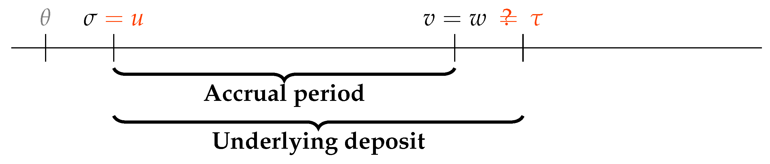
A vanilla LIBOR coupon referencing a LIBOR fixing is characterised by four dates: the fixing date , the coupon accrual start date u, the coupon accrual end date v and the payment date w. The LIBOR fixing date is the same for the fixing and the coupon and is the link between them. For vanilla coupons, the start accrual date is equal to the underlying deposit effective date, i.e., . Some swaps coupons, in particular with corporates, have an effective date delayed by a couple of days. For the deposit maturity date and the coupon end accrual date, one would like to say that they are also the same, but this is not always the case due to non-good business days adjustments. The coupons accrual dates are separated by a regular periods, e.g., three months, with each date in the list adjusted for non-good business days. When the start date of an accrual period is adjusted but the end date is adjusted by fewer days, the accrual period does not have a length equal to the theoretical period but a slightly shorter one. On the other side, the dates for the deposit underlying LIBOR are computed for each fixing separately, taking only into account the relevant start date and end date of the theoretical period, and not the adjustment done on the derivative. This can be described by “LIBOR means LIBOR” and LIBOR is not influenced by where it is used. In practice, the end accrual date and theoretical maturity dates coincide () except when a non-good business day intervenes. This non-coincidence appears roughly for two coupons out of seven (Saturdays and Sundays are non-good business days) where there is one day difference and ( minus one business day). The payment is done at the end of the accrual period in . The LIBOR fixing figure, which we denote , is known in , and the amount, which consists of the rate multiplied by the accrual factor, denoted as , is paid only in . The different dates are represented in Figure 1.
The option pricing in continuous time using the equivalent martingale measure approach provides a generic method to price contingent claims. The technical details of the approach can be found for example in (Hunt and Kennedy 2004, Corollary 7.34) for the underlying mathematics and in (Henrard 2014, Theorem 8.1) for the application in presence of collateral.
We apply the generic pricing approach to contingent claims referencing a LIBOR rate fixed in and paid in w. Note that the fixing is -measurable, even if paid only in .
Theorem 1.
In a economy satisfying the standard conditions (see Hunt and Kennedy 2004), the present value of a contingent claim with payoff in w is given in by
where is the collateral cash-account, is the market-price-of-risk-adjusted (or risk-neutral) measure and is the filtration representing the information available in s.
For a LIBOR coupon as described above, the valuation formula gives
A FRA presents a picture similar to vanilla coupons in term of dates, except that the payment takes place in u (not in v) and the amount paid is adjusted by a discounting-like formula. For a fixed rate K, the amount paid in u is
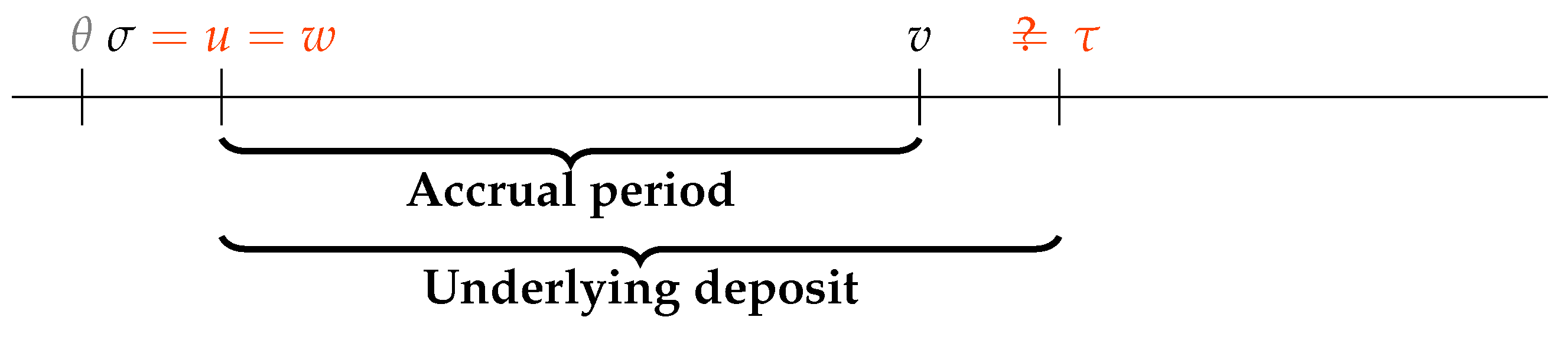
Note that the formula above is not a valuation/modelling choice but part of the term sheet, the legal contract signed by the parties. The different dates associated with a FRA are represented in Figure 2.
The value of s is given in the standard option valuation framework by
The FRAs are only one example of instruments with a similar date pattern where the payment takes place in , the deposit effective date, and not in , the maturity date. Other instruments include LIBOR-in-arrears and some exotics products such as range accruals. We emphasise that the payment date occurs in , which is several months before . As the fixing rate is -measurable with , the current FRA term sheets do not have a measurability problem. The -measurability of allows instruments referencing them to use that information at any date on or after . Many instrument’s term sheets use that flexibility and it seems natural that any replacement of for exiting contracts should respect that feature.
The LIBOR-like benchmarks are currently the most important benchmarks in the interest rate derivative markets, but there exists another type of benchmarks that takes more and more importance and that is expected to replace the LIBOR benchmarks to some extent; they are the overnight benchmarks.
The overnight benchmarks are similar to LIBOR benchmarks in the sense that they measure some level of interest rate on a given deposit term. The main difference is that for overnight benchmarks the term is reduced to a single night; the rate is for a deposit from today to the next good business day.
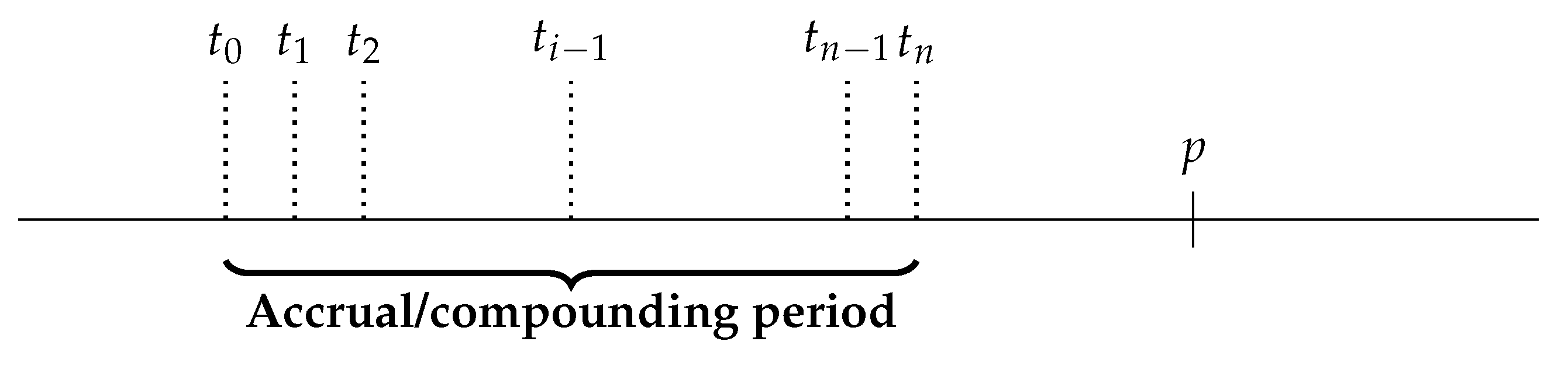
Associated to those overnight benchmarks is a type of derivatives called Overnight Indexed Swaps (OIS). The floating coupons of those instruments are not paid on a daily basis, even if the underlying benchmark is for a single day. The rates are accumulated by composition and paid after a certain term. If we denote by a set of -consecutive business days, representing n one-day periods and the overnight fixing for the period and the associated accrual factors, the amount paid on an OIS floating coupon (for a notional of 1) is the composition
The payment takes place in p which is usually one or two good-business days after the last day of the period . This lag is required for a smooth settlement of the amount paid. The representation of the dates is proposed in Figure 3.
3. Fallback and Expected Value
The valuation formula (Equation (1)) is written as if the LIBOR benchmark were always published in and thus available for payment in w. The current expectation, described in the Introduction, is that the benchmark may stop being published at some stage. We denote the announcement date of the discontinuation by a and the discontinuation date itself by d. Those dates are still unknown and can be modelled with stopping times. If a discontinuation were to take place, in today’s legal wording of the contract, there is no guarantee that something meaningful would replace the LIBOR figure. The actual valuation formula should be
The question mark in the formula is not a typo, it is really an uncertainty related to the legal framework in the case of cessation of the LIBOR and the actual cash flow in that state of the universe would be highly uncertain.
Industry groups have gathered to find a practical way to replace that question mark by something manageable. Most of the derivative market is governed by ISDA master agreements or by CCP rule books inspired by it. ISDA (2018b) has launched a consultation on ways to amend the master agreements from July to October 2018 and the preliminary results of the consultation have been published on 27 November 2018 and later detailed in ISDA (2018a). This initial consultation was covering a limited number of currencies (AUD, CHF, GBP, and JPY). Another consultation ISDA (2019) took place from May to July 2019, mainly related to USD and its preliminary results have been published on 30 July 2019, while the full results have not been published yet at the time of writing. To some extent, what will be decided by the ISDA Benchmark Committee will become the de facto standard for the derivative market.
The general idea of the fallback would be to substitute the LIBOR fixing in the derivatives by a new quantity obtained as the sum of an adjusted RFR and an adjustment spread. The former would play the role of the floating rate; it would depend on an overnight benchmark and be known around the date where LIBOR should have been fixed (the precise rules are described below). The latter, the adjustment spread, would be decided when the discontinuation is announced and be seen as an adjustment to avoid value transfer between the original LIBOR fixing and the new fixing mechanism. The new pricing formula becomes
The quantity is the adjusted RFR that replaces ; we use a notation with the date to indicate that the figure is associated to the original one fixed in but it should not be interpreted as being -measurable. We show below that, in the main ISDA proposal, it is actually not -measurable.
The spread S will be based on some historical mean or median. The notation for the spread contains two types of indications. The X and the length l represents a set of parameters that still have to be decided by the ISDA Benchmark Committee. Those parameters are not related to the derivatives themselves or the interest rate market; they are contractual descriptions such as the choice between mean and median, a potential trimming of the values and transitional period. To some extent, the contracts have been signed already by the market participants but some terms still have to be decided by the Committee. The spread will be fully known on the announcement date and will depend on historical data from a certain look back period l—which could be a 10-year period or another period to be decided—before the announcement. We have represented that period by the time interval .
4. Adjusted RFR
The ISDA proposal for the adjusted RFR is to use a compounding setting in arrears approach. The composition is given by
The proposal sounds reasonable as it would replace a quantity that would no longer exist () by an accumulation of elements that still exists () using an accumulation mechanism (composition) familiar in the derivative market and natural for interest rates. Unfortunately, the proposal suffers major flaws that can be summarised as lack of details and lack of measurability2. The flaws described here are related only to the fallback procedure, not for new trades referencing directly the overnight benchmarks. For new trades, one can make sure that the term sheet has all the required details and that the dates are compatible.
In Equation (6), what would be the dates and with respect to the dates , , , u, v and w described in Section 2? As the adjusted RFR is a replacement of LIBOR, it should be based only on LIBOR related dates and not on the derivative specific dates. The most natural ones would be that , the fixing date, is completely ignored and the overnight composition is done on the theoretical deposit period of the LIBOR, with and . In this way, all the occurrences of LIBOR are replaced with the same figure. Even if this is natural, this precision is not given in the ISDA documents—neither in the consultation document, nor in the document describing the results. The reason of the absence of the precision can probably be seen in Figure 1 and Figure 2. The payment date w is, in many cases, before the end of the theoretical deposit in . The minimal requirement is that the amount paid is known when paid, i.e., that is -measurable. This requirement is not satisfied with the natural choice of dates described above. The measurability requirement may appear as a technical term of no practical importance, but it is not; it is only the precise description of a very practical requirement that before you are able to pay an amount, you need to know what amount should be paid.
A less natural approach to the date’s choice would be to use and . This is less natural as such an approach would lack coherence. The same LIBOR figure would be replaced by different numbers, depending on where it is used. Moreover, even with the second approach, the issue of the upfront payment, as in the FRA case, could not be solved. In that case, the payment is done in u before any information about the composition figure is known. Without precise dates, the proposal cannot be implemented and when precise dates are used, it appears that the proposal is simply not achievable.
Several workarounds have been proposed unofficially to deal with this fundamental flaw. They include changing the term sheet of FRA to bring the payment to the end date v. It would solve the FRA problem in the most favourable case () but not the one of other products with a similar payment schedule like LIBOR in-arrears. Other proposed mechanisms include a “cut-off” period at the end of the composition, where a couple of days before the end date , the same rate would be used for a couple of days (k days) and the payment formula would become
with and . This may solve the measurability question when there is only a couple of days discrepancy but would introduce significant valuation and risk management issues, e.g., curve intra-month seasonality and convexity adjustments. This does not appear to be a reasonable workaround.
Those issues have been publicly (e.g., Henrard 2019a) and privately mentioned and have been debated in industry magazine (e.g., Sherif 2019a, 2019b) and public podcast.3 This is not simply an oversight of some trivial details, but a fundamental flaw in the proposal that has been exposed for a while and for which an answer is still missing. ISDA has indicated that the exact wording of the fallback will be published for consultation in 2019 and with a target implementation in 2020. Given the lack of attention to details in previous documents and the lack of answer to precise information requests, in the opinion of this author, it is doubtful that a satisfactory solution will be provided.
On the other side, a potential robust solution to the adjusted RFR rate in the fallback has been proposed by different working groups and this author. The solution is based on an OIS benchmark, also called forward-looking rate or term RFR. The solution has the favour of the majority of the market participants, when offered the possibility to chose it. On the EUR side, this was in particular the result of a recent consultation organised by the Working Group EUR Risk-Free Rates (2019). On the GBP side, a recent statement of the Working Group on Sterling Risk-Free Reference Rates published on the Bank of England website indicated that “the RFRWG also supports work currently underway to develop a term benchmark based on the sterling risk-free rate”. This solution was surprisingly not included in the ISDA consultation. A recent letter by the same institution to the FSB4 appears to warn participants with harsh (and possibly unwarranted) words against this solution. At this stage, this new benchmark does not exist and one has to be prudent not to recreate the issue we are trying to escape from. The inclusion of term rate could be done through a waterfall fallback as the one recommended by ARRC working groups for FRN5, securitisation and business loans with the term rate the waterfall’s first step. This single step is not a panacea, but to obtain a realistic solution, one has to accept to discuss the problem’s full complexity, its constraints and review all the potential solutions.
The alternative solution is based on forward looking OIS rates. On the fixing date , the fair fixed rate for an OIS with effective date and maturity date is measured. The adjusted RFR would be that OIS rate, i.e.,
This is a forward-looking or market expectation view of the same composition quantity used in the officially proposed method. If we ignore the difference between the maturity date and the payment date p, the value of the rate can be computed simply from (pseudo-)discount factors by
as proved in (Henrard 2014, Section 8.3.3). The impact of the payment in p instead of on the rate was proved to be negligible in practice in Henrard (2004).
Those instruments are fairly liquid in the market and the numbers above are quoted continuously on Swap Execution Facilities (SEF) and Multilateral Trading Facilities (MTF). To incorporate this approach in practice, one would need to discuss the difference between the end accrual date and the OIS payment date p (and adjust or not for it). However, in general, this approach is well-defined with the measurability of the same as the one of —both are -measurable—and the mechanism from which the number is obtained is very familiar to the derivative market (OIS fair rate).
The solution has clear advantages and the support of a large part of market participants. Its main disadvantage is that such a benchmark does not exist yet. However, similar benchmarks, such as the ICE Swap rate6, are widely used and there is a general consensus that such an OIS benchmark would be viable, including by A. Bailey as reported in Rega-Jones (2019).
Note that, when both approaches—the compounded setting in arrears and the forward looking term rate—are achievable in practice, the valuation and risk management of both approaches before the fixing date are the same. It is only after the fixing date that the approaches differ; the OIS benchmark is achievable, has the same measurability and has a similar risk profile to the one of the original LIBOR coupon while the compounded setting in-arrears may not be achievable and generate a significantly different risk profile.
We prove that the two approaches are equivalent in valuation terms before the fixing date .
Theorem 2.
The prices of a overnight linked coupon with compounding setting in-arrear or a standard coupon fixing on the OIS benchmark are equal before the fixing date θ of the OIS benchmark:
Proof.
The present value of the OIS benchmark approach is, using the measure associated to the collateral account,
The first equality uses the tower property of conditional expectation. The second equality uses the fact that is -measurable (Equation (9)) for the adjusted RFR and the definition of . The last equality uses the martingale property of .
The cash flow in the backward-looking option is also paid in but based on the composition of the daily rates compounded over the period. Today’s value of the payment is given by
The first equality is obtained from (Henrard 2014, Theorem 2.4) and is the pricing of vanilla OIS. The reasoning leading to that result is a little bit long and involves multiple nested conditional expectations and for that reason is not reproduced here; we refer to the above reference for the details. □
5. Adjustment Spread
The adjustment spread is denoted by . This is to indicate that it depends on methodology parameters X still to be decided and on some market data obtained in the period preceding the announcement date with l the look back period. In some sense, all the LIBOR derivatives are now path dependent up to the discontinuation’s announcement date.
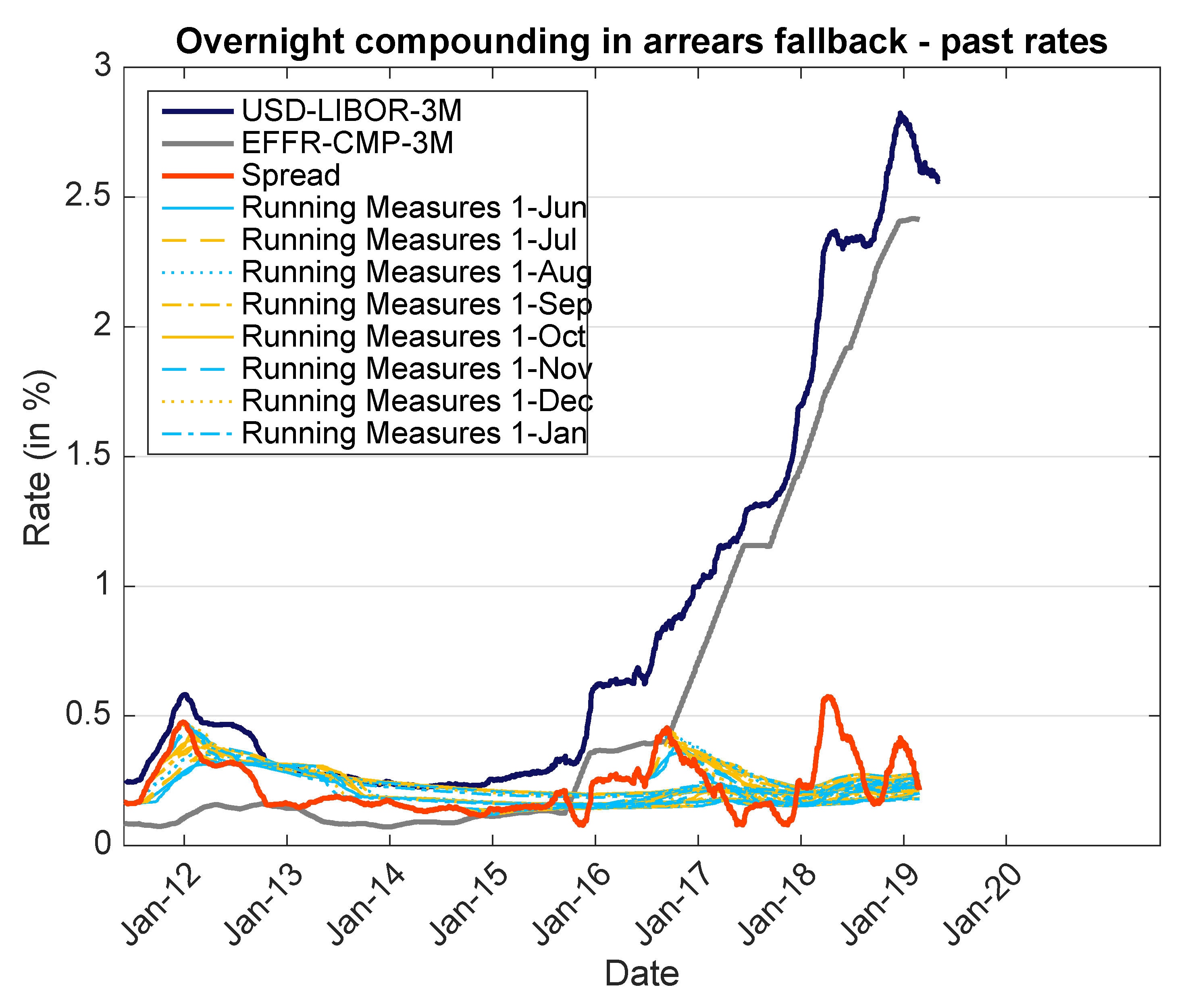
The expected methodology to compute the spread S is based on historical data, and in particular the daily spread (difference) between and with and . Note the already mentioned difference in measurability between which is -measurable and which is -measurable. The computed spread is coming from a difference in credit riskiness between the two different types of benchmarks but also from a difference between forecasted and realised rates. The spread is more volatile than a simple credit analysis would suggest and embeds unexpected monetary policy actions, as seen recently in the US. Figure 4 displays historical data where this volatility can be observed.
The fallback mechanism includes some market information—in Equation (5), we formally represent the information available by the filtration —but also some information about the methodology as discussed by the Committee members. That information about the discussion is generally not available to the public and is only available to the people privy to the methodology selection process. The existence of those different sets of information is not only a theoretical hypothesis but a fact recognised in practice by ISDA. In a recent letter7, the association indicates the valuation sensitivity of those parameters and the requirement to hide it from market participants8.
It means that there are in fact at least two filtrations, the pure financial market one, which we denote , and a second one, containing more information and that we denote from now on by : . The second filtration contains the information related to the methodology choices. Some people have access to and generic market participants only to . Applying the two filtrations in Equation (5) would generate different prices. It is not clear in general which value will be higher, as the hidden information can lead to lower or higher estimates of the spread. However, better information allows the market participant privy to that information to buy or sell at a better price. This situation can be compared, from an information point of view, to the situation of material non-public information in the securities market.
Note that the expected date for the LIBOR discontinuation is around the end of 2021 and the look back period could be ten years. This would means that from the period , almost 80% of the relevant data—the period [2011, 2019]—is already known. It makes the value of the information in the hidden parameters X even higher.
Equation (5)—and similar formulas writing the present value as an expectation of future cash flows—emphasises one element which appears misunderstood. The changes on the amounts or , even if the exact quantities will be known only in a or in w, have already an impact on the present value of the instruments today. There is no need to wait the actual discontinuation in d to feel the changes of value. In the standard valuation framework used in this note, the present value of derivatives is the expectation of the discounted payoff; changing the payoff has an immediate impact on the present value and creates immediate value transfer. The value transfer started as soon as the discussions on the changes in the fallback wording started.
Each new information, in or , has a direct impact on the present value. If one market participant has the information and acts on it, he will change the market value immediately by his demand or offer. Even if the only information one other participant has is , he will be able to see a discrepancy of value between his estimation of value from and the market value partly based on . It does not provide him the full information contained in but at least an indication that such an information may exist and be known by other market participants. It is important that a strong governance procedure is in place to avoid the extra information contained in to be abused.
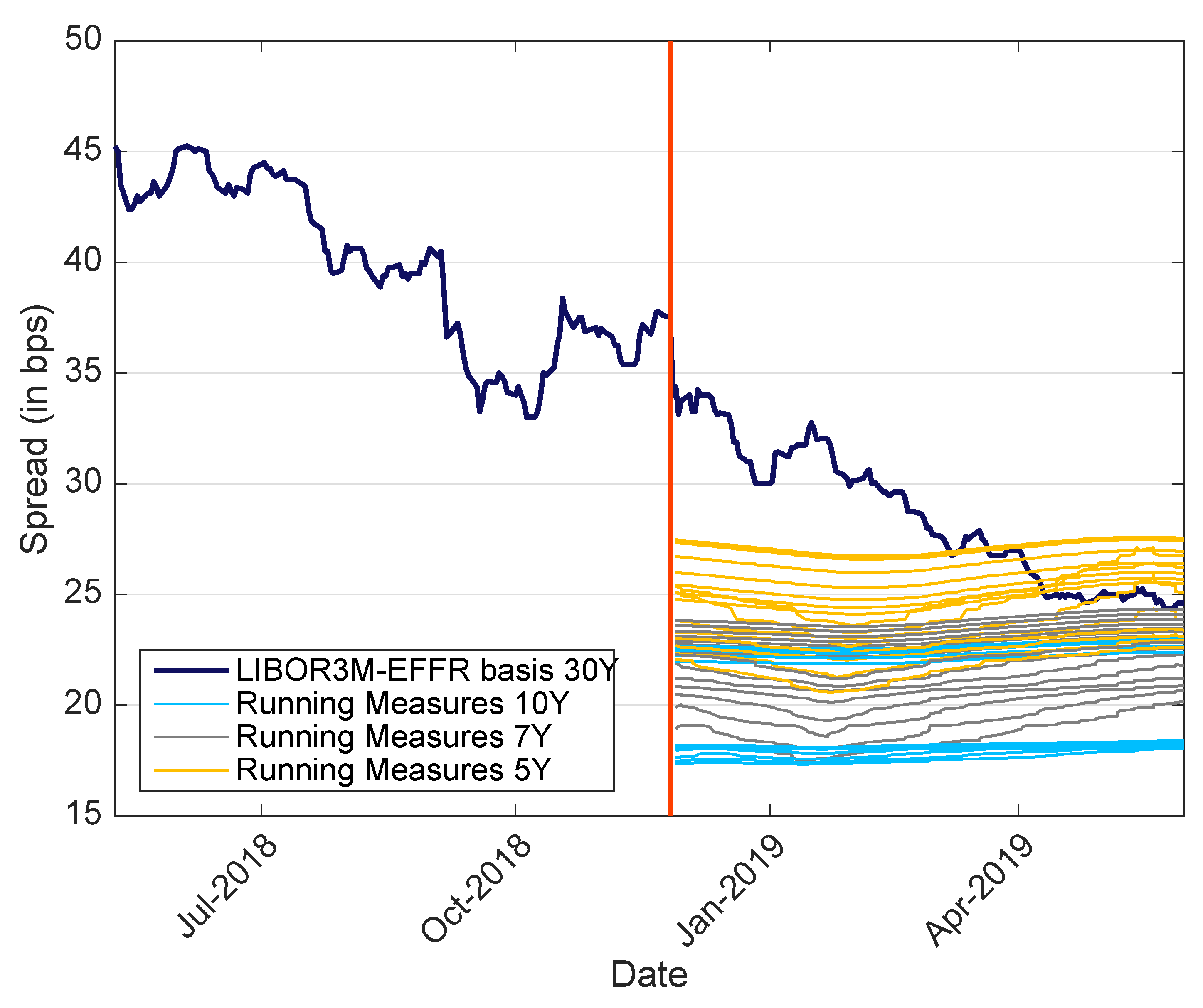
This is a situation that some market participants may have felt last November. The market value of some instruments started to deviate significantly from their previous value without new economical information beside the small and natural incoming of incremental information from the passing of time. In a couple of days, we went from to with limited important economic news. On the other side, the price of some derivatives linked to LIBOR, in particular the basis spread between LIBOR and OIS, changed dramatically in that couple of days. This could be an indication that a particular discrepancy between and had appeared. This change of price is represented in Figure 5. The graph displays the spread of basis swaps between USD-LIBOR-3M and average EFFR9. The spread moved significantly in the days after 26 November 2018 when the results of the consultation were known and the change of spread continued for the several months following that date, always in the same direction. It is only if a new set of information, not related to the economy in general but related to the information contained in the ISDA consultation results, is introduced that the market moves make sense. The graph depicts the market data of the spread—in dark blue thick line—and this author’s best guess of what the spread would be based on past data and hints in the ISDA documents. The best guess is based on 48 scenarios (median/mean, eight potential announcement dates and three potential look back periods). For each scenario, a thin line represents the mean/median computed with past data on that date, i.e., it is the information about S available using public information about the methodology. The choice of the historical approach was public only on 26 November 2018, and we reproduce the running average only from that date onward. In some sense, the lines represent the part of available to this author on any given date. As the methodology is further clarified in the future, the number of scenarios will decrease and the range of possibilities will narrow.
The historical data related to the spread is depicted in Figure 4. A large part of the historical average/median for the 5, 7 or 10 years preceding the potential announcement is already known. The market that was pricing the spread at around 37 basis points for USD-LIBOR-3M/EFFR just before the consultation results—already down from around 45 basis points a couple of months before—has now moved to 25 basis points. It appears that it took roughly three months for the market participants to move their valuation paradigm from to . It is likely that some market participants had access to the information but did not figure its impact on pricing immediately. Incorporating the extra information from the consultation explains the market move with surprisingly good precision10. A brief summary of figures for USD and GBP with three- and six-month tenors is provided in Table 1. All the spreads have move significantly over the last months. The GBP ten-year means are strongly impacted by the 2012 period. We can expect the mean to decrease slightly in the coming months.
According to the author’s data, the standard deviation of the USD-LIBOR-3M/EFFR spread has been divided by 2.5 between the period before November 2018 and the last three months. It is difficult to unentangle the macro-economic situation from instruments specific movements. One cannot prove the origin of those movements, but the joint movements in different currencies and the significant jump on a specific date are presumptions in favour of the explanation provided above. The coming months will show if the spreads stabilise at the expected fallback levels.
Note also that the historical spreads that will be used are between the forward-looking LIBOR and the backward-looking composition on overnight. It includes the past credit spread but also the past misestimations of future monetary policy decisions. If the adjustment spread is to obtain a neutral value transfer for the introduction of the fallback, it should be computed between the forward-looking LIBOR and a measure of forward-looking OIS when the fallback is introduced. Viewed from today or from the announcement date, both rates are forward looking and the adjustment spread should be based on forward-looking methodologies. Even if the past is a perfect estimator of the future, it is not clear that the spread methodology proposed is the correct one. The forward-looking OIS versus backward-looking composition can be hedged at zero cost with market swaps and should probably not be included in the spread computation.
6. Options and Hedging
The fallback introduces a new payoff for products currently linked to LIBOR. Some natural questions related to this new payoff type are: Which parts of it can be hedged? What is the dynamic of the different parts of the payoff (, , d, and )? Can we obtain enough information about the implied dynamics from the market?
The easiest part to start with is . In both approaches discussed in Section 4, the figure is based on compounding overnight rates. One is setting in arrears and one is forward-looking, but, as proved in Theorem 2, in term of valuation and risk management before the fixing, the two are equivalent. The OIS market exists and is liquid to some extent. Hedging this part is not an issue. The dynamic side is more involved. Currently, there is no liquidity in option-like products—cap/floor or swaptions—with overnight benchmarks as an underlying. It is impossible to obtain directly precise implied dynamic from the market.
The second observation is regarding the LIBOR with fallback inside Equation (5). If we take the full quantity, including the pure LIBOR and the overnight alternatives, the associated market is liquid. Swaps, cap/floor and swaptions on LIBOR with fallback are still the most liquid interest rate instruments. Even if the actual fallback wording has not been penciled explicitly yet and no contract includes this to-be-created wording yet, the general expectation is that, as soon as the wording is definitive and included in new contracts through updated master agreements, CCPs will change their rule books to include the fallback, for legacy trades as well as new contracts as described in LCH (2018). It is also expected that the large banks will sign protocols to apply the new wording/payoff to their legacy contracts. Even if the contracts have not been written yet and even less signed, from a valuation perspective, one can consider that the new payoff is already in place. If one believes that the discontinuation will actually take place by 2022, he has to consider that the long-term instruments are actually already overnight benchmarks-based and the dynamic of the LIBOR with fallback is actually the dynamic of the overnight-linked products. This provide a positive indirect answer to the question of the previous paragraph that had a negative direct answer: for post-2021 payoffs, the prices and implied dynamics of LIBOR linked products are actually prices and implied dynamics of OIS-like products.
We can try to go further into the details of those payoffs. For the announcement date a and the discontinuation date d themselves, there is a market expectation, at least for the ICE LIBOR in different currencies, that the discontinuation will take place around the beginning of 2022—1 January 2022 was used in the scenarios presented in the previous section—and the announcement date will be a couple of months before that. However, there is no instrument depending on that outcome on its own. There are no such things as binary swaps on those dates, e.g., an instrument paying a fixed amount if LIBOR exists and nothing otherwise. A similar reasoning can be done for the methodology parameters X and l; there is no market instrument where each component can be priced in isolation. The fact that most bilateral derivatives trade under similar master agreements and that CCPs will transfer the wording in their rule books means that there is uniformity of payoff among all liquid derivatives. If there were several fallback methodologies planned, for example with different spread approaches, one could try to extract from the differences in price the market implied values of some of those elements. However, from the uniformity, we can only price LIBOR and its fallback as a combined item and not each component separately.
Maybe going outside the derivative world, e.g., to Floating Rate Notes (FRN) or securitisation, could offer more information on the fallback elements as their fallback wording is different. However, for each individual FRN, there is an underlying credit and convenience yield impact. Even if the fallback is different, this difference, which is expected to be relatively small, will be lost in the idiosyncratic features of each note. It seems there is no practical possibility to extract information on the fallback from them.
Obviously, there will be no LIBOR after its discontinuation and asking what would be the value of for does not make sense. However, we could try to use a proxy to estimate the credit risk impact that is removed by the fallback. Some benchmark providers have started to publish benchmarks that somehow represent bank credit and could be used as a proxy, e.g., US Dollar ICE Bank Yield Index11 or Ameribor®12, but there is no derivative trading currently on those indices and there is also no practical possibility to extract any information from them.
Consequently, there is no real hope to obtain the market implied information on the fallback details for the derivatives. There is no real hope to compute a precise amount for the value transfer resulting from the disappearance of LIBOR and its fallback choice and even less to hedge it. The valuation impact, positive or negative, from the fallback choice on end-users with a net exposure to LIBOR will probably remain unknown.
7. Conclusions
The LIBOR fallback is first and foremost a legal challenge. Nevertheless, writing it in the language of quantitative finance helps not only to estimate the potential impacts in term of value transfer, but also to understand what is possible and what is not. In the opinion of this author, this approach that helps clarify the issues has been neglected in the current discussions. The ensuing lack of precision has pushed the discussions to an impasse. The current proposals cannot be implemented in practice due to lack of measurability. A fundamental revision of the foundations of the fallback is required. Each workaround not taking into account the quantitative finance foundations of the problem leads to further issues that appear to be without simple and elegant solution. A simple and elegant solution to the fallback has been proposed, under the form of an OIS benchmark adjusted RFR, but appears to be resisted for derivatives.
On the other hand, the difference in access to information related to the fallback methodology by different market participants has created a non-level playing field that can be described technically by the existence of two parallel filtrations for the pricing of financial instruments. If some participants were allowed to act on the richer filtration, an uncontrolled value transfer between market participants may ensue.
The goal of this note is to describe requirements for a technically achievable fallback process. To reach the goal of implementing an achievable fallback, one has to accept to discuss the problem full complexity, its constraints and review all the potential solutions. If the note achieves that goal it will quickly become de facto obsolete; an achievable precise fallback mechanism will be implemented and its origin can be forgotten.
For quantitative analysts, a second phase, consisting in developing model specific estimation of value transfers and developing new payoffs and models compatible with the new market, will start.
Funding
This research received no external funding.
Conflicts of Interest
The author declares no conflict of interest.
Abbreviations
The following abbreviations are used in this manuscript:
| ISDA | International Swaps and Derivatives Association |
| LIBOR | London InterBank Offered Rate |
| EFFR | Effective Federal Fund Rate |
| SOFR | Secured Overnight Financing Rate |
| FRA | Forward Rate Agreement |
| OIS | Overnight Indexed Swap |
References
- Bailey, Andrew. 2017. The Future of LIBOR. Speech at Bloomberg London. Available online: https://www.fca.org.uk/news/speeches/the-future-of-libor (accessed on 11 August 2019).
- Duffie, Darrell. 2018. Compression Auctions with an Application to LIBOR-SOFR Swap Conversion. Technical Report. Stanford: Graduate School of Business, Stanford University. [Google Scholar]
- Henrard, Marc. 2004. Overnight Indexed Swaps and Floored Compounded Instrument in HJM One-Factor Model. Ewp-fin 0402008, Economics Working Paper Archive. Munich: University Library of Munich. [Google Scholar]
- Henrard, Marc. 2014. Interest Rate Modelling in the Multi-Curve Framework: Foundations, Evolution and Implementation. Applied Quantitative Finance. London: Palgrave Macmillan, ISBN 978-1-137-37465-3. [Google Scholar]
- Henrard, Marc. 2019a. Fallback Compounding in Arrears Won’T Work! Multi-Curve Framework Blog Post. Available online: http://multi-curve-framework.blogspot.com/2019/03/fallback-compounding-in-arrears-wont.html (accessed on 11 August 2019).
- Henrard, Marc. 2019b. A Quant Perspective on IBOR Fallback Consutation Results. Market Infrastructure Analysis. muRisQ Advisory. Available online: https://ssrn.com/abstract=3308766 (accessed on 11 August 2019).
- Hunt, Philip J., and Joanne E. Kennedy. 2004. Financial Derivatives in Theory and Practice, 2nd ed. Wiley Series in Probability and Statistics; Hoboken: Wiley. [Google Scholar]
- ISDA. 2018a. Anonymized Narrative Summary of Responses to the ISDA Consultation on Term Fixings and Spread Adjustment Methodologies. Consultation Results. New York: The Brattle Group—ISDA. [Google Scholar]
- ISDA. 2018b. Consultation on Certain Aspects of Fallbacks for Derivatives Referencing GBP LIBOR, CHF LIBOR, JPY LIBOR, TIBOR, Euroyen TIBOR and BBSW. Consultation, ISDA. Available online: https://www.isda.org/2018/07/12/interbank-offered-rate-ibor-fallbacks-for-2006-isda-definitions (accessed on 11 August 2019).
- ISDA. 2019. Supplemental Consultation on Spread and Term Adjustments for Fallbacks in Derivatives Referencing USD LIBOR, CDOR and HIBOR and Certain Aspects of Fallbacks for Derivatives Referencing SOR. Consultation, ISDA. Available online: https://www.isda.org/a/n6tME/Supplemental-Consultation-on-USD-LIBOR-CDOR-HIBOR-and-SOR.pdf (accessed on 11 August 2019).
- LCH. 2018. LCH’s Position in Respect of ISDA’s Recommended Benchmark Fallback Approaches. LCH Circular No. 3999. Available online: https://www.lch.com/membership/ltd-membership/ltd-member-updates/lchs-position-respect-isdas-recommended-benchmark (accessed on 11 August 2019).
- Lyashenko, Andrei, and Fabio Mercurio. 2019. Looking Forward to Backward-Looking Rates: A Modeling Framework for Term Rates Replacing LIBOR. Technical Report. Amsterdam: Elsevier. [Google Scholar]
- Pomberg, Stefan, and Sander Willems. 2019. Back to a single curve? State of play of alternative risk-free rates. Paper presented at the QuantMinds International 2019, Hamburg, Germany, May 11–15. [Google Scholar]
- Rega-Jones, Natasha. 2019. FCA: Sonia Derivatives Liquid Enough to Create Term Rates. Available online: https://www.risk.net/derivatives/6712261/fca-sonia-derivatives-liquid-enough-to-create-term-rates (accessed on 11 August 2019).
- Schrimpf, Andreas, and Vladyslav Sushko. 2019. Beyond LIBOR: A Primer on the New Reference Rates. BIS Quarterly Review. Basel: Bank for International Settlements. [Google Scholar]
- Sherif, Nazneen. 2019a. FRAs Won’t Work with Standard Libor Fallback, Experts Say. Available online: https://www.risk.net/derivatives/6453341/fras-wont-work-with-standard-libor-fallback-experts-say (accessed on 11 August 2019).
- Sherif, Nazneen. 2019b. LIBOR-In-Arrears Swaps Face Unwinds on Benchmark Death. Available online: https://www.risk.net/derivatives/6572906/libor-in-arrears-swaps-face-unwinds-on-benchmark-death (accessed on 11 August 2019).
- Working Group EUR Risk-Free Rates. 2019. Second Public Consultation by the Working Group on Euro Risk-Free Rates: On Determining an ESTER-Based Term Structure Methodology as a Fallback in EURIBOR-Linked Contracts. Consultation, European Central Bank. Available online: https://www.ecb.europa.eu/paym/cons/html/wg_ester_term_structure_methodology.en.html (accessed on 11 August 2019).
- Zhu, Haoxiang. 2019. The Clock Is Ticking: A Multi-Maturity Clock Auction Design for LIBOR Transition. Presentation at Planning for the end of LIBOR, Cass Business School. Available online: https://www.cass.city.ac.uk/__data/assets/pdf_file/0004/471757/15h_Haoxiang-Zhu_LIBORCass.pdf (accessed on 11 August 2019).
| 1 | We use the term LIBOR to designate benchmarks related to interbank lending. Sensu stricto, the term LIBOR is restricted to the benchmarks administered by IBA and fixing in London. By abuse of language, we extend it in this note to other similar benchmarks such as EURIBOR, TIBOR, BBSW, etc. |
| 2 | Thanks to Andrea Macrina for pointing this way to describe the measurability problem. |
| 3 | |
| 4 | Letter available at https://www.isda.org/a/Y6SME/April-2019-Letter-to-FSB-OSSG.pdf. |
| 5 | Document available at https://www.newyorkfed.org/medialibrary/Microsites/arrc/files/2019/FRN_Fallback_Language.pdf. |
| 6 | See the administrator website at https://www.theice.com/iba/ice-swap-rate. |
| 7 | Text available at https://www.isda.org/a/Y6SME/April-2019-Letter-to-FSB-OSSG.pdf. |
| 8 | The exact wording is: ISDA to work with The Brattle Group and other external experts to analyse and perform sensitivity analysis on the “historical mean/median approach” to the spread adjustment (without input from ISDA working groups or market participants during this time period given the sensitivity of the parameters). |
| 9 | The target replacement for USD-LIBOR is SOFR, but the liquidity of SOFR based swaps is currently very limited and it is proxied here with EFFR. The difference in the current market is a couple of basis points. |
| 10 | Similar results have been obtained for the CHF, GBP markets and and USD-LIBOR-6M. The CHF data are described in Pomberg and Willems (2019). The GBP and some USD data are not depicted in this note but can be found on the author’s blog at http://multi-curve-framework.blogspot.com/. |
| 11 | See description at https://www.theice.com/iba/Bank-Yield-Index-Test-Rates. |
| 12 |
Figure 1.
Representation of the dates associated to a LIBOR fixing and a LIBOR coupon in a vanilla IRS.
Figure 1.
Representation of the dates associated to a LIBOR fixing and a LIBOR coupon in a vanilla IRS.

Figure 2.
Representation of the dates associated to a LIBOR fixing and a FRA instrument.

Figure 3.
Representation of the dates associated to an OIS.

Figure 4.
Historical time series for USD-LIBOR-3M and EFFR compounded on three-month periods. Running mean and median are for 5-, 7 -and 10-year look back periods and different announcement dates.
Figure 4.
Historical time series for USD-LIBOR-3M and EFFR compounded on three-month periods. Running mean and median are for 5-, 7 -and 10-year look back periods and different announcement dates.

Figure 5.
Historical time series for long tenor (30-year) basis swaps USD-LIBOR-3M/EFFR around the ISDA consultation period. The red vertical line is the consultation result date. The different thin lines are the author’s estimates using scenarios with different methodologies.
Figure 5.
Historical time series for long tenor (30-year) basis swaps USD-LIBOR-3M/EFFR around the ISDA consultation period. The red vertical line is the consultation result date. The different thin lines are the author’s estimates using scenarios with different methodologies.


Table 1.
Spread between the different LIBOR indices and overnight composition. The spreads at the different dates are the market spreads for 30-year tenor basis swaps similar to those reported in Figure 5 for USD-LIBOR-3M. The ranges represent the author’s estimates for the different scenarios.
Table 1.
Spread between the different LIBOR indices and overnight composition. The spreads at the different dates are the market spreads for 30-year tenor basis swaps similar to those reported in Figure 5 for USD-LIBOR-3M. The ranges represent the author’s estimates for the different scenarios.
| Index | July 2018 | November 2018 | May 2019 | Range |
|---|---|---|---|---|
| USD-LIBOR-3M | 45 | 38 | 25 | (18–28) |
| USD-LIBOR-6M | 57 | 50 | 35 | (30–40) |
| GBP-LIBOR-3M | 27 | 22 | 17 | (10–17) |
| GBP-LIBOR-6M | 33 | 28 | 24 | (18–32) |
| Spreads in basis points. | ||||
© 2019 by the author. Licensee MDPI, Basel, Switzerland. This article is an open access article distributed under the terms and conditions of the Creative Commons Attribution (CC BY) license (http://creativecommons.org/licenses/by/4.0/).
Share and Cite
MDPI and ACS Style
Henrard, M.P. LIBOR Fallback and Quantitative Finance. Risks 2019, 7, 88. https://0-doi-org.brum.beds.ac.uk/10.3390/risks7030088
AMA Style
Henrard MP. LIBOR Fallback and Quantitative Finance. Risks. 2019; 7(3):88. https://0-doi-org.brum.beds.ac.uk/10.3390/risks7030088
Chicago/Turabian StyleHenrard, Marc Pierre. 2019. "LIBOR Fallback and Quantitative Finance" Risks 7, no. 3: 88. https://0-doi-org.brum.beds.ac.uk/10.3390/risks7030088
Note that from the first issue of 2016, this journal uses article numbers instead of page numbers. See further details here.