Stochastic Mortality Modelling for Dependent Coupled Lives


1
Institute for Financial and Actuarial Mathematics, Department of Mathematical Sciences, University of Liverpool, Liverpool L69 7ZL, UK
2
African Institute for Mathematical Sciences Ghana, Legon, P. O. Box LGDTD 20046 Accra, Ghana
*
Author to whom correspondence should be addressed.
†
These authors contributed equally to this work.
Risks 2020, 8(1), 17; https://0-doi-org.brum.beds.ac.uk/10.3390/risks8010017
Submission received: 3 December 2019
/
Revised: 31 January 2020
/
Accepted: 5 February 2020
/
Published: 11 February 2020
(This article belongs to the Special Issue Interplay between Financial and Actuarial Mathematics)
Abstract
:Broken-heart syndrome is the most common form of short-term dependence, inducing a temporary increase in an individual’s force of mortality upon the occurrence of extreme events, such as the loss of a spouse. Socioeconomic influences on bereavement processes allow for suggestion of variability in the significance of short-term dependence between couples in countries of differing levels of economic development. Motivated by analysis of a Ghanaian data set, we propose a stochastic mortality model of the joint mortality of paired lives and the causal relation between their death times, in a less economically developed country than those considered in existing studies. The paired mortality intensities are assumed to be non-mean-reverting Cox–Ingersoll–Ross processes, reflecting the reduced concentration of the initial loss impact apparent in the data set. The effect of the death on the mortality intensity of the surviving spouse is given by a mean-reverting Ornstein–Uhlenbeck process which captures the subsiding nature of the mortality increase characteristic of broken-heart syndrome. Inclusion of a population wide volatility parameter in the Ornstein–Uhlenbeck bereavement process gives rise to a significant non-diversifiable risk, heightening the importance of the dependence assumption in this case. Applying the model proposed to an insurance pricing problem, we obtain the appropriate premium under consideration of dependence between coupled lives through application of the indifference pricing principle.
1. Introduction
1.1. Review of Existing Literature
Two lives involved in the pricing of an insurance contract are conventionally regarded as being mutually independent, inferring there exists no relationship between their remaining lifetimes. Although this assumption induces greater simplicity in pricing calculations through reduction of the joint life estimation problem to the estimation problem of a single life, it does not reflect reality. Addressing the existence of dependence between the lifetimes of two individuals holding a joint insurance contract is therefore important in improving the accuracy of insurance product pricing. Survival probabilities of two members of a married couple whose remaining lifetimes are considered to be dependent at the initiation of the policy may vary in line with the status of their partner’s life. Mortality laws determined at the time of the policy’s valuation dictate the calculation of prospective provisions; however, a change in circumstance in regard to the survival of two dependent lives during the contract may alter the value of the agreement, due to a change in the bereaved spouse’s probability of survival.
Approaches to modelling dependence between the times of death of paired lives vary across the literature. One method frequently applied in dependence structure modelling is to use copulas to express the joint survival functions of interest. Many papers including those by Frees et al. (1996); Youn and Shemyakin (1999), Carriere (2000); Denuit et al. (2001) and Shemyakin and Youn (2006) implement copulas in modelling the dependence structures of joint lives. Under the assumption dependence between lifetimes is induced by a mutually experienced external event affecting both members of a couple, common shock models are an alternative to the copula approach introduced by Marshall and Olkin (1967) and discussed by Frees et al. (1996) when testing the robustness of their selection of the Frank copula with Gompertz marginals. The proportional hazards survival model implemented by Hougaard et al. (1992) when investigating the relationship between mortality rates of twins across generations incorporates time dependent explanatory variables into the analysis whilst accounting for common shared frailties.
Markov chain methods are implemented in various works as a basis for joint mortality models. Subsequent to the loss of a spouse, it is likely that the bereaved will experience adaptations in their living conditions due to factors inclusive of grief and stress. Martikainen and Valkonen (1996) propose such changes contribute to the interdependence of the lifetimes of paired lives. Norberg (1989) models the progression of the marital status of two coupled lives over time using a continuous time four state Markov chain, allowing for the incorporation of such a dependence structure by setting marital status as a determining factor of the force of mortality, in addition to age and sex. Spreeuw and Wang (2008) expand Norberg’s model to a six state Markov chain, introducing an intermediate time period for each spouse within which the bereaved may remain for at most some specified time, prior to transitioning to the following surviving state. This modification enables investigation of the short-term dependence structures commonly associated with coupled lives, of which broken-heart syndrome is the most common.
One limitation of the model proposed by Spreeuw and Wang (2008) is that in moving between time periods the bereaved spouse experiences a sudden jump in mortality intensity, when in reality this change would be smooth. Semi-Markov chain models have superior flexibility in comparison to the standard Markov chain model, and time since previous transition is a determining factor in calculation of transition probabilities in addition to current time and state occupied. Ji et al. (2011) define broken-heart syndrome as a smooth parametric function of the time since bereavement through implementation of a semi-Markov model, enabling greater information gain in regard to how the broken-heart syndrome effect changes with time. It is clear that model selection influences the pricing and valuation of insurance products. The Markov chain model proposed by Norberg (1989) suggests the mortality intensity of the bereaved spouse increases permanently; however, the semi-Markov model described by Ji et al. (2011) allows for the bereaved spouse to recover following the initial death, thus facilitating duration dependence.
Financial risk, alongside systematic and unsystematic mortality risk, are the fundamental risk factors insurers are exposed to (Dahl 2004). Milevsky and Promislow (2001) present a more realistic modelling approach compared to prior assumption of constant interest in previous studies. Implementation of a Cox–Ingersoll–Ross interest rate process with stochastic force of mortality specified by a mean-reverting Brownian Gompertz process, enables incorporation of both interest rate and systematic mortality risk in their model.
Deterministic mortality intensities defined as functions of the age of the policy holder have traditionally been used by actuaries in the pricing and valuation of insurance products. Stochastic modelling of mortality forms an alternative class of mortality models; however, much of the literature focuses only on single cohort mortality. The use of stochastic processes in modelling mortality intensity allows for incorporation of the uncertainty of future mortality development and time dependence in the mortality model, enabling improvements in the accuracy and likelihood of realistic calculations, in addition to allowing for quantification of the mortality risk faced by insurance companies.
Paralleling mathematical approaches to modelling time to default discussed in credit risk literature, Dahl (2004); Biffis (2005); Luciano and Vigna (2005); Schrager (2006) and Luciano and Vigna (2008) model the remaining lifetime of an individual as a doubly stochastic stopping time of a Cox process, with stochastic intensity given by the force of mortality. Suggestion of a link between credit-sensitive securities and insurance contracts was initially proposed by Artzner and Delbaen (1995), enabling exploitation of similarities between both time to default and remaining lifetime and short-term interest rate and force of mortality.
Credit risk models can generally be classified into two distinct model categories (see Jarrow and Protter (2004) for comparison). Originating from the approaches of Black and Scholes (1973) and Merton (1974), structural models focus on the structural characteristics of an institution when considering default risk, comparing the market value of a company’s assets to their liabilities with complete knowledge of a comprehensive information set. The approach of the aforementioned literature falls into the class of reduced form models, implemented without the need to account for company specific factors underlying the occurrence of a default due to assumption of an exogenous cause (Saunders and Allen 2002).
In the case of the joint mortality experience of coupled lives, Luciano et al. (2008) again adopt the reduced form credit risk methodology, implementing a continuous time cohort model of affine type. The paper creates the first link between stochastic and copula based approaches through application of an Archimedean copula for the modelling of dependence between survival times of coupled lives. Archimedean copulas are popular in the modelling of joint lifetimes since bivariate distributions generated by frailty models are a subclass of this particular copula family (Oakes 1989). Luciano et al. (2016) find two parameter extensions of Archimedean copulas to be more suitable for representing coupled dependence when investigating the dependence of spouses across generations.
Frequent assumption of symmetric mortality reactions and the staticity of dependence over time are two of the drawbacks of copula use, with the continuous density assumption common to this approach implying no jump in mortality occurs on the loss of a spouse. Spreeuw (2006) investigates the nature of dependence and time-dependent association between lifetimes through implementation of a number of single parameter Archimedean type copula models. Almost all copulas selected exhibit long-term dependence, with just one family presenting short-term dependence for only young ages or short durations. Pure short-term dependence was not recognised in any of the copulas studied; however, a limitation of single parameter models in capturing all dependence classes was proposed, in line with Luciano et al. (2016). Allowing for asymmetric mortality reactions to the occurrence of a death, Gourieroux and Lu (2015) introduce jumps in mortality intensity through combination of a Freund model with an unobservable common static frailty representing the socioeconomic conditions shared by coupled lives. Additional dependence between lifetimes further to the contagion effects resulting directly from the loss is therefore generated through implementation of their model. Although dependence due to unobserved risk factors is not considered by Dufresne et al. (2018), incorporation of age difference and sex of the elder spouse in definition of the level of association between coupled lifetimes in a copula model, supports suggestion of asymmetric dependence.
Jevtić and Hurd (2017) introduce an alternative to copula dependence in the credit risk environment through definition of a probabilistic mechanism describing the influence the primary death has on the bereaved spouse. A stochastic mortality model of affine type is implemented for mortality experience, assuming correlated non-mean-reverting Ornstein–Uhlenbeck diffusions for the mortality intensities of coupled lives. This selection satisfies the requirements discussed by Cairns et al. (2006) detailing criteria for a good stochastic mortality model. Strong mean-reversion should rule out the selection of a model, even if the target level is time dependent and incorporates mortality improvements. Inclusion of mean-reversion in the modelling of mortality intensities requires a diminishing likelihood of future mortality improvements in the event that recent mortality developments occur at a faster rate than anticipated. Uncertainties surrounding medical advances and improvements in the healthcare and pharmaceutical industry highlight the unsuitability of a mortality model with such constraints. In line with this, existing research suggests time-homogeneous mean-reverting affine processes do not fit observed mortality tables, whilst forces of mortality appear to behave exponentially rather than in a mean-reverting fashion (Luciano and Vigna 2005).
In relation to credit risk, however, default intensities are generally modelled as mean-reverting processes. As such, implementation of the classical Cox–Ingersoll–Ross model is popular within credit risk literature. The Feller process is a non-mean-reverting adaptation of the classical Cox–Ingersoll–Ross model. In contrast to Ornstein–Uhlenbeck-type processes, the non-negativity constraint of mortality intensity is not violated through implementation of this model, conditional on the non-negativity of the initial starting point. Following calibration of a Feller model carried out by Luciano and Vigna (2008), survival probability was found to decrease at every age, an additional advantage of the selection, whilst inclusion of a rooted mortality intensity tempers the volatility of the process. We combine the non-mean reverting Cox–Ingersoll–Ross and Ornstein–Uhlenbeck stochastic processes to form the joint mortality model proposed. Many applications of these processes appear in the financial and insurance mathematics literature, and the interested reader may refer to Liang et al. (2011); Nowak and Romaniuk (2018) and Dassios et al. (2019) for examples of such applications.
1.2. Broken-Heart Syndrome and Shared Frailty Dependence
Broken-heart syndrome is a medically recognised condition triggered by severe negative events such as the loss of a spouse. The death induces a jump in the mortality rate of the bereaved spouse experienced at the moment of the primary death. Mortality elevation is generally greatest during the first period of bereavement after which a significant reduction occurs. Historical research into the prevelance of broken-heart syndrome suggests the elevated mortality of the surviving spouse diminishes significantly following an approximate period of between six and twelve months (Rees and Lutkins 1967), (Parkes et al. 1969), (Ward 1976), falling to the commonly lower mortality of the comparative non-widowed population in some cases. Factors influencing the impact of broken-heart syndrome include the cause of death of the deceased spouse (Elwert and Christakis 2008), the age of the bereaved spouse and the location of the first death (Rees and Lutkins 1967), with widowers experiencing a greater change in mortality when compared to that of widows.
Allowing for the existence of dependence between two lives involved in an insurance contract, Frees et al. (1996) and Carriere (2000) provide indications of strong positive correlation between death times of coupled lives. The presence of dependence suggests joint life annuities making payments until the first loss of life are underpriced, whilst last survivor annuities providing benefits until the final death are overpriced (Spreeuw and Wang 2008). Considering dependent lives Frees et al. (1996) identify a reduction in value of a joint-life annuity of approximately 5% compared to standard models under the assumption of independence. Spreeuw and Wang (2008) compare models with and without dependence of mortality on time elapsed since death of the spouse to the independence case, observing the need for higher premiums for a contingent insurance contract with dependent lives. When time is factored into the dependence, however, lower premiums were noted, with the mortality drop characteristic of broken-heart syndrome outweighing the initial mortality elevation. Similar trends in regard to the impact of the mortality pattern were found when pricing a reversionary annuity; however, independence yields increased premiums in this case due to the shorter period of payments associated with an increased degree of dependence.
Dependence duration should be established to determine the full extent of pricing implications. Hougaard (2000) discusses the classification of dependence across three time frames, with time elapsed since the death of the deceased allowing for differentiation between the three classes. Characterised by an elevated force of mortality which is a decreasing function of time since death, broken-heart syndrome is the most recognised form of short-term dependence. Long-term and instantaneous dependence, also referred to as the common shock effect, constitute the remaining classifications which should be considered by insurers in the pricing of products involving mortality assumptions. For further details on the definition of each dependence structure, see Hougaard (2000).
The true nature of the impact of spousal bereavement is a consideration of significant importance to insurers in regard to both pricing and the exploitation of opportunities for diversification, with relations between the remaining lifetimes of paired lives found to exist prior to death through unobserved couple-level frailties (Klein 1992). Spurious risk dependence refers to dependence due to unobserved heterogeneities associated with each member of a couple. In contrast to broken-heart syndrome which is causal by definition, spurious risk dependence between lifetimes is solely attributable to the sharing of correlated risk factors or frailties. Living conditions, healthcare access, diet habits and mutual emotional stresses are amongst some of the lifestyle features which may act as determinants of both health and mortality, with suggestion of selectivity in the formation of couples implying the pairing of individuals with equivalent levels of risk, heightening the prevalence of such correlation. Improvements in underwriting processes within an insurance company and diversification of insurance portfolios would allow for minimisation of this dependence risk in the event correlated unobserved heterogeneities are the main component of spousal mortality dependence. Identification of a marked causal effect of spousal bereavement would however require addressing, since assumption of coupled mortality dependence would be needed across all insured populations regardless of their characteristics.
Implementing a mixed proportional hazards model with flexible semi-parametric distribution for the unobserved heterogeneities, Lu (2017) separates the two dependence factors whilst allowing for both positive and negative spurious risk dependence. Comparison of models with and without consideration of spurious correlation using French joint annuity data reveals 92.4% and 81% of the mortality jump observed in bereaved males and females, respectively, is accounted for by broken-heart syndrome, whilst the remainder reflects the impact of the unobserved heterogeneity. Despite the dominance of broken-heart syndrome over spurious correlation, disregarding either effect was found to produce significant pricing errors. van den Berg et al. (2011) provide evidence for the causal effect of conjugal bereavement on mortality and health, reporting a reduction in residual life expectancy of 12% on average following the loss of a spouse. In line with Lu (2017), the model proposed acknowledges the error in assuming the life status of an individual’s spouse to be an exogenous determinant of mortality. Allowing for correlated unobserved heterogeneities and applying joint models of survival van den Berg et al. (2011) capture both causal and spurious dependence, reporting an increased mortality of greatest significance during the first two and a half years of bereavement which then decreases up to five years post loss, at which point the effect is no longer present. Applications of shared frailty models can also be seen in relation to both twin mortality and chronic disease incidence, with inclusion of a common risk factor accounting for the unobserved heterogeneities; for further details, refer to Clayton (1978) and Hougaard et al. (1992).
Although the negative implications of the loss of a spouse on the remaining lifetime of the bereaved partner are widely accepted, there exists a suggestion of differences in cultural patterns of bereavement reactions (Osterwers and Solomon 1984), (Parkes et al. 2015). Factors recognised by psychologists as determinants of cultural differences among populations (Laungani 1996), environmental features and sociological ideas such as those linking periods of economic, social, or political change to the absence of recognised norms and the associated influence on mental health (Durkheim 1897) are supportive of this hypothesis. In carrying out this study, we are particularly interested in the identification of sociological influences on joint mortalities and of variation in dependence structures between coupled lives in differing cultural settings.
Knowledge of the importance of insurance in sustaining economic growth has a history of significant length (United Nations 1964); however, penetration in low and lower-middle income countries remains reduced in comparison to higher-middle and high income countries (Outreville 2013), with determinants of consumption ranging from income per capita, inflation and banking sector development to religious inclination (Beck and Webb 2003). As a long-term savings instrument and measure of risk mitigation providing protection against the financial consequences of death, the need for increased life insurance penetration rates in such economies is highlighted by its connection with financial development levels (Outreville 1996). The importance of acknowledging dependence between coupled lives particularly in low and lower-middle income countries and consequently alleviating the insurance risk associated with inaccurate pricing mechanisms is therefore heightened by this connection, due to the instability of the associated economies.
1.3. Novelty of the Approach
Considering for the first time to the best of our knowledge the existence of socioeconomic influences on dependence between coupled lives and the bereavement process of surviving spouses in less economically developed populations, we utilise analysis of a Ghanaian dataset within which a lesser initial concentration of broken-heart syndome is observed to inform the proposal of a joint mortality model. In line with our observations which fit the nature of a reduced volatility and following the results of Luciano and Vigna (2008), we introduce correlated non-mean-reverting Cox–Ingersoll–Ross diffusions as paired mortality intensities, defining a model of the joint mortality of a couple assumed to share the same socioeconomic environment based on the stochastic mortality model proposed by Jevtić and Hurd (2017). A mean-reverting Ornstein–Uhlenbeck process is selected to represent the influence the loss of a spouse has on the remaining lifetime of the surviving partner. In moving from deterministic to stochastic bereavement, we facilitate a potential non-diversifiable risk requiring a premium which accounts for the change in mortality observed in the data, unlike the diversifiable nature of risks associated with a deterministic bereavement process.
Observation of an increased mortality during the first period of bereavement paired with the findings of Lu (2017) suggests dependence between lives within the sample is mostly causal in nature. Existence of a cause-and-effect relationship between the remaining lifetimes of paired individuals is therefore captured in the proposed model through definition of the bereavement effect, whilst couple specific unobserved heterogeneities are accounted for through inclusion of correlated Brownian motions in the paired mortality processes.
An outline of the paper is as follows, in Section 2, we discuss data supporting the modification of mortality processes before introducing the mortality model proposed in Section 3. One example of pricing a life insurance product incorporating the dependence model is provided in Section 4 alongside a numerical pricing example. Concluding remarks are given in Section 5.
2. Data Set
Evaluation of the existence of the broken-heart syndrome effect requires data which details the time of death of both members of a couple. Survey data collected at the University of Ghana is used to motivate the model proposed in this paper. Questions relating to the grandparents of a sample of students at the university include their number of children, living situation and the circumstances of their death in addition to the date at which they died.
Data processing revealed the full data set comprises 246 couples, 38 couples failing to have experienced at least one death were removed from the sample since the waiting time between deaths is the variable of interest. Couples corresponding to errors within the data collection were removed, in addition to outliers and those with incomplete data in regard to time of death. This leaves a total of 145 couples consisting of 61 double deaths and 84 single deaths, with 37 and 52 male first deaths, respectively. Since a number of bereaved spouses survived the observation period determined by the survey completion date, the data are said to be right-censored. The survival curve for the sample is displayed in Figure 1, with censored data points indicated.
Figure 2a,b show the distribution of male and female death times within a couple, whilst Figure 2c illustrates the number of deaths per year of bereavement. A total of eight bereaved spouses died within the first year of bereavement, corresponding to 13.1% of bereaved individuals in the sample. Although the death rate decreased to 5 out of the 61 bereaved spouses in the second year of bereavement, eight deaths were again observed in year five. Couples along the red line in Figure 2b are those exhibiting the classical features of broken-heart syndrome, with survival time less than one year.
The Pearson correlation between male and female deaths is 0.362773 when considering the whole sample; however, since year of birth range for the male spouse subset is approximately 55 years, the data were split into two cohorts to test for existence of a generational effect. Figure 3 and Figure 4 correspond to the cohorts of paired lives such that male year of birth falls in the intervals 1899–1926 and 1927–1954, respectively. After removal of outliers and couples with incomplete date of birth, 29 couples remained in cohort one and 28 couples in cohort two.
During the first year of bereavement, five surviving spouses died in cohort one, representing 17.2% of the bereaved sample. Following a drop in the number of deaths upon survival of the first year, a second peak of four deaths was observed in year four. The proportion of bereaved deaths experienced in the second cohort was 10.7% during the first year of bereavement with the deaths of three bereaved spouses, and reached a maximum of 21.4% with six deaths in year five. In addition to the differing patterns of bereaved deaths observed in Figure 3 and Figure 4, with the older cohort achieving its peak frequency much later, the Pearson correlation between male and female deaths within the sub-samples varies significantly. Correlation coefficients are −0.008397 and 0.4188 in the first and second cohorts respectively, suggesting the existence of a potential change in reactions to bereavement across generations.
A second data set was collected at the African Institute for Mathematical Sciences in Rwanda. Following exclusion of couples within which either one or both spouses were alive, the sample consisted of 38 couples from a total of 12 African countries. Due to construction of the survey in this case, the data collected reveals only intervals within which the survival time corresponding to each couple lies, although the maximum number of deaths once more occurs within the first period of bereavement.
Taking interval extremes and considering the upper bound of survival time, 23.7% of the bereaved sample died in the third year of bereavement with a second peak of 15.8% in year six, whilst 26.3% of the bereaved sample died in the first year when assuming the lower bound of survival time followed by 18.4% in year two, with no further peaks. The Pearson correlation between male and female deaths was fairly low with values of −0.2250 and −0.06755 for the upper and lower bounds, respectively, initiating consideration of the existence of country specific trends. Within this analysis, couples of Cameroonian and Ghanaian origin appear to behave in a similar fashion, whilst paired death times corresponding to Rwandese couples are widely distributed. The occurrence of mass death events such as the Rwandan genocide in 1994 may be proposed as potential causes of disruption in the general mortality pattern. Although the results perhaps imply the impact of broken-heart syndrome differs across developing countries, further analysis is required in relation to this hypothesis since it is difficult to draw such a conclusion from a data set of this size.
Previous investigations into the impacts of the effect have to the best of our knowledge regarded a group originating from a developed country as their sample population. Rees and Lutkins (1967) discuss their findings following an investigation into the mortality of bereaved close relatives. The number of deaths documented vary significantly from the control group in the first year of bereavement, with 11.6% of deaths followed by the death of a close relative in comparison to just 1.6% in the control. Subsequent to this, the percentage of total deaths in the bereaved group falls to a rate of 1.99%, not differing significantly from the comparative non-bereaved rate.
Focusing specifically on the effect of a death within a married couple, Rees and Lutkins (1967) found that fitting with the general trend of the data the severity of increases in mortality were greatest during the first year of bereavement, after which the magnitude of rate elevation diminishes. The mortality rate of widowers within the year following the loss of the deceased was 19.6%, a value sizeably greater than the same rate for widows (8.5%). In the case of widowers, the pattern of changing mortality differs slightly from the general findings of the investigation, 13.7% of widowers at risk died within the first six months following the bereavement whilst just 5.9% died in the second, a difference in mortality found to be significant at the 1% level.
Frees et al. (1996); Carriere (2000); Youn and Shemyakin (1999); Shemyakin and Youn (2006); Spreeuw and Wang (2008); Luciano et al. (2016) and Dufresne et al. (2018) are amongst a number of studies making use of data from a large Canadian insurer. Observations include increased mortality for widows and widowers in comparison to non-widowed lives, maximum mortality rates among individuals having lost their partner less than one year ago and the implication of a greater influence of broken-heart syndrome on men rather than women.
Although Ghanaian survey data supports the suggestion that broken-heart syndrome exists in countries of all levels of development, comparison with existing literature prompts the proposal behaviour under broken-heart syndrome may differ. The significant decrease in mortality following survival of the first year of bereavement is a characteristic prevalent in much of the research in this area; however, the decreasing trend of mortality with increasing year since bereavement, although apparent, cannot be identified with such high initial concentration and decay rate in the Ghanaian data. Such dissimilarities lead us to define a mortality model representing the impact of a dependence with less immediate significance. In the following section, we introduce the model proposed before considering the impact of assumption of dependence on the pricing of joint-life insurance products in Section 4.
3. Model Description
Inclusion of the probabilistic framework in the stochastic mortality model proposed by Jevtić and Hurd (2017) prompted the decision to implement a similar model within our investigation. Whilst multiple state models such as the semi-Markov chain model applied by Ji et al. (2011) offer transparency and the ability to observe whether the level of risk changes following a death event, the probabilistic mechanism also enables incorporation of the health of both members of a couple prior to the primary death. This feature increases the accuracy of the dependence model by permitting varied responses to the initial death, where dependence may be irregular across the population, determined by the health circumstances of each couple under consideration. Although we focus on the short-term dependence of coupled lives, the model proposed is capable of addressing both short- and long-term structures, with the ability to encompass any existence of dependence between two lifetimes before the death of one spouse. In this section, we propose an adaptation of the stochastic mortality model with probabilistic framework described by Jevtić and Hurd (2017), first defining a number of important concepts for survival analysis.
Fundamental in modelling mortality risk, the survival function of an individual aged x, referred to as , specifies the probability the individual survives for at least t years and is defined by
where is the remaining lifetime of . Manipulation of this function allows for calculation of the force of mortality, such that
where is the force of mortality of for , describing the instantaneous rate at which the individual experiences death. The force of mortality of an individual at time 0 is given by
Analagous to the pricing at time t of a default-free zero-coupon bond with maturity , under the assumption of a credit risk setting, the conditional probability of a stopping time exceeding some arbitrary time , where is doubly stochastic with intensity , can be shown to satisfy
where represents the information at time t. When implemented in mortality modelling, the stopping time often represents the remaining lifetime of an individual.
3.1. Probabilistic Mechanism
Let be a complete probability space where is a filtration satisfying the usual conditions of right continuity and completeness, large enough to carry a d-dimensional Brownian motion W, two exponentially distributed random variables and , and a single uniformly distributed random variable U. Within this space, the set is fully independent, with a realisation of the time of death of each partner following from every realisation of the randomly generated elements. Allowing T to represent a finite time horizon of suitable length, the Brownian filtration is defined over the interval and is given by for , where is a sub-filtration of . When applying the model to a sizeable population, an index , where N is the number of couples in the sample, should be added to every element whose properties are specific to a particular pair.
Consider two coupled lives aged x and y at time 0 with future lifetimes and , respectively. The instantaneous forces of mortality at time t given by for , are predictable -adapted processes driven by the Brownian motion W. The spouse whose death occurs first is identified as the deceased partner and denoted . Equivalently, the spouse who survives the first death is denoted q and labelled the bereaved partner. The remaining lifetime of spouse p, conditional on the information set , is the first jump-time of a nonexplosive inhomogeneous Poisson counting process N with parameter , where counts the number of deaths at time t, for . The remaining lifetime of spouse q is defined in an analogous manner, with both doubly stochastic stopping times representing and driven by the sub-filtration .
The first time of death is therefore given by
whilst the uniform random variable U allows for identification of the deceased spouse through comparison with a function of the forces of mortality at the instant of the primary death. Recalling that p is the label given to the partner who dies first, we have
In line with the belief the loss of a spouse has an impact on the mortality of the surviving spouse, is defined for as the mortality intensity of the bereaved partner following the initial death. This force of mortality is an adjustment of the original and the association between the two rates reflects the influence losing a partner has on the bereaved spouse’s health and hence their remaining lifetime. The bereavement effect is described by
the change in mortality process, where the modified process is inclusive of a structural break at representing the instant effect on the bereaved spouse’s mortality. The instantaneous rise at the first death time is given by a linear combination of the mortality of each spouse at time directly before the death, such that
where coefficients and are assumed to be non-negative. Intuitively, the mortality jump reflects the short-term dependence structure of broken-heart syndrome and modification of the adaptations in the mortality intensity of the surviving spouse due to adjustments in the life circumstances of the bereaved. Inclusion of the mortality intensity of both spouses in the estimation of the bereavement jump given in Equation (5) allows for incorporation of unobserved shared frailties.
Determined using a similar approach to the first time of death , the second time of death is given by
The model proposed is a variation of the reduced form modelling approach frequently used in the study of credit risk to model default as a stopping time whose occurrence is unexpected. Implementation of this method in regard to dependencies of bereaved partners suggests a change in the remaining lifetime of the bereaved spouse does not occur following the primary death, since random variables used in the determination of the time of death of each spouse , are required to be independent across the index. Inclusion of the modified intensity resolves this limitation.
Determination of the structure of dependence across a population may be of interest in addition to dependence between a particular couple. To model the dependence relationship amongst a whole population, risk factors experienced commonly by all individuals and risks specific to each member of the population should be considered. These factors are labelled systematic and idiosyncratic risks, respectively, and are an independent collection of factors by construction, with correlation between individuals induced by the risks shared among those under consideration.
The objective of the probabilistic mechanism is to determine the joint probability density function for the times of death of two coupled lives . Theorem 1 provides an expression for the joint density proposed with proof in Jevtić and Hurd (2017), where expectations are taken under the probability measure and it is assumed the death events do not occur simultaneously.
Theorem 1
(Jevtić and Hurd (2017)).
- 1.
- The joint probability density function for the time of death of two coupled lives is given by the reduced form expression
- 2.
- The marginal probability density function for the time of the first occurring death isfor
3.2. Stochastic Mortality Model with Non-Mean-Reverting Cox–Ingersoll–Ross Mortality Processes
It is common practice in financial modelling to assume the stochastic mortality intensity to be an affine process, due to their analytical tractability. Under sufficient technical conditions, the affine assumption gives rise to the expression
where and are unique functions satisfying generalised Riccati ordinary differential equations. Owing to the convenience of affine jump-diffusions, we propose a stochastic mortality model under the assumption of affine mortality intensities, assuming a cohort of single-life mortality models in continuous time with correlated, non-mean-reverting Cox–Ingersoll–Ross (CIR) processes representing the paired mortality intensities and . For further discussion and treatment of affine processes, see Duffie et al. (2003).
The adapted CIR processes are defined by
where the parameters , , and are positive. Let be a three-dimensional Brownian motion; each Brownian motion and can then be considered as a linear combination of two independent Brownian motions such that
which gives
Here, and represent the random idiosyncratic risk factors specific to each member of the couple and reflects the random couple specific risk factors commonly experienced by both members of the pair, an example of which is the mutual living environment often shared by coupled lives. Weights and are selected in order to satisfy , where and is the Pearson correlation between and . Introducing correlation between the two Brownian motions in this way allows for dependence prior to the initial death and enables the capturing of unobserved heterogeneities assumed to be shared between coupled lives.
Remark 1.
Selection of population specific risk factors for representation in the component of the Brownian motions and rather than the couple specific risks assumed in this paper initiates a non-diversifiable risk to insurers, creating with certainty, a long-term effect for companies which should be considered in the pricing and valuation of insurance products.
The final step in establishing the model is to define the bereavement effect explicitly, since determination of the second death time requires inclusion of the modified process , for . With correlation between coupled lives reflected in the paired Brownian motions, the bereavement model explains the causal relation between remaining lifetimes and the true contagion effect of the loss of a spouse. Specification of the bereavement process determines the dependence structure assumed to exist between the lives of interest, such flexibility in the model allows for consideration of all dependence classifications as required. Jevtić and Hurd (2017) define as a deterministic function with dynamics given by
for values of t greater than the initial time of death . In the deterministic case, the law of large numbers implies diversification of the risk associated with the loss of a spouse, we therefore propose an alternative approach to modelling the bereavement jump facilitating the existence of a non-diversifiable bereavement risk such that the associated premium must account for the change in mortality experienced after the first death. We fix coefficients and of Equation (5) at zero for computational simplicity; however, selection of positive values for and allows for incorporation of the mortality intensities of both lives prior to the first death in the initial value of the bereavement effect at time .
Definition 1.
The change in mortality process has dynamics given by an Ornstein–Uhlenbeck process such that
where is an independent d-dimensional Brownian motion, and .The explicit solution of the bereavement process for is
We assume the bereavement process defined in Definition 1 to be of affine type to allow for computation of the joint probability density function.
Remark 2.
The volatility of the bereavement process driven by the Brownian motion in Equation (12) is a determining feature of the nature of dependence. Fixing across the whole population infers the occurrence of an event experienced individually by all bereaved spouses at some future point in time. Such an event induces a non-diversifiable risk, posing a significant threat to the insurance industry in practice and creating the need for premiums which account for the observed change in mortality. On the other hand, assumption of a couple specific value for means the future event risk is diversifiable, through the insuring of a large and varied sample of couples.
Selection of as either fixed or varying should be determined through observation of data. Establishing a more detailed underwriting process would help in the identification of unobserved heterogeneities, reducing the dependence risk associated with this component of the bereavement process. Estimation of the volatility in Equations (9) and (11) may also be facilitated through increased data collection; however, since the existence of a future event common to all lives is not apparent in the data set analysed, we assume to be couple specific, acknowledging the possibility that a more populated data set may support the need for a change in this assumption.
When pricing a reversionary annuity in Section 4, the volatility coefficient does not appear in the indifference price. Since the risks associated with the correlated Brownian motions are diversifiable through inclusion of only couple specific risk factors, this independence of is of no concern in our case. In the non-diversifiable case discussed in Remark 1, however, the initial value of the bereavement effect given in Equation (11) should be redefined in order to incorporate both and the causal dependence between the members of each couple, to ensure the price of the insurance product covers the risk associated with a spousal loss.
Remark 3.
The Brownian motion of the bereavement process is assumed to be independent of the paired Brownian motions associated with mortality intensity. If the Brownian motion in Equation (11) is instead given by , the change in mortality of the surviving spouse upon the death of their partner is assumed to be correlated with their mortality before the primary death. The independence assumption adopted in this paper increases the importance of random risks, such as environmental factors, in determination of the impact of the loss, rather than historical mortality. The existence of dependence between the bereavement process and the mortality of the surviving spouse before the death at time , although an interesting concept, is not considered in this paper.
In the Ornstein-Uhleneck model of bereavement proposed, the mean reversion parameter is fixed at zero due to the decreasing significance of the mortality gap over time associated with the subsiding nature of the mortality elevation, characteristic of broken-heart syndrome. In contrast to the exponential model of bereavement assumed in Jevtić and Hurd (2017), mean reversion allows for the process to take both positive and negative values, accounting for instances when the mortality of the bereaved improves in comparison to a non-widowed mortality.
After establishing the structure of the bereavement effect, expectations required for the joint probability density and survival function calculations can be computed through application of the affine framework with term structure equation determined by the Feynman–Kac formula. The conditional formula whose specific form is used in the calculation of bond prices (see, for example, Grasselli and Hurd (2015)), is given by
where and are constant and for .
Proposition 1.
Three corollaries follow Proposition 1 whose proof is detailed in Appendix A. The explicit form of the expectations of interest under conditions appropriate in the mortality context are given in Corollary 1, whilst Corollaries 2 and 3 provide expressions for the joint probability density and survival functions, respectively. For proof of Corollary 2, see Appendix B.
Corollary 1.
The specific form of the conditional formula required for calculation of both the probability density and survival functions occurs when constants and are fixed at 1 and 0, respectively, which gives
and
where
and
Throughout the remainder of the paper, we will refer to functions and as and , respectively.
Corollary 2.
The joint probability density function for death times and with bereavement process of Ornstein–Uhlenbeck type is given by the expression
for , where , and are as defined in Corollary 1, and and are unique functions satisfying the generalised Riccati ordinary differential equations for the Ornstein–Uhlenbeck bereavement process , such that
and
Evaluating the derivatives of and with respect to in line with Proposition 1 and Corollary 2, gives
and
For further details on calculation of the joint probability density function, refer to Appendix B. and are as computed in Jevtić and Hurd (2017).
Remark 4.
The joint probability density function for the case is analogous to Corollary 2, with indices interchanged.
Under the assumption of independent coupled lives, the convenience of the affine environment allows for the survival probability of an individual aged x to be given by
Due to the changing mortality of the bereaved spouse upon the initial death at time , consideration of dependent lives requires the redefinition of the survival function in Equation (28). We instead regard the survival function for to be the product of two survival functions, split at the first jump time such that
Therefore, in accordance with the affine process selection for mortality intensity, the expression
holds for , whilst the survival probability for is determined through application of the law of total probability, which leads to Corollary 3.
Corollary 3.
The survival probability of an individual assuming a mortality intensity of non-mean reverting Cox–Ingersoll–Ross type is given by
where is defined by Equation (21).
Remark 5.
The survival probability of spouse is analogous to the survival probability of spouse detailed in Corollary 3, with indices interchanged.
One example of incorporating the model proposed in the pricing of a joint-life insurance contract using the indifference pricing principle approach is given in the following section.
4. Indifference Price Calculation for a Joint-Life Insurance Product
When pricing in the incomplete financial market setting, the utility indifference principle is an approach introduced by Hodges and Neuberger (1989) which compares the maximal expected utilities of an investor with and without taking a risk. Initially implemented in the pricing of European options and motivated by the unrealistic assumption of no transaction costs in the pure Black–Scholes model, extensions of the method have since been developed by Davis et al. (1993) and Ludkovski and Young (2008) among others, with the latter considering mortality contingent claims in a fully stochastic setting. In relation to life insurance, such an approach involves equating the expected utility of an insurer when a certain number of insurance policies are written to the expected utility when such policies are not written. The indifference premium of interest to our research is the change in premium which should be charged when dependence of coupled lives is assumed.
Various articles detail application of the indifference principle to pricing in the life insurance sector. Young and Zariphopoulou (2002) implement the approach in the valuation of insurance risks in the dynamic financial market setting. Extensions of their results are presented by Delong (2009) and Liang and Lu (2017) who follow similar procedures in order to determine indifference premiums. Liang and Lu (2017) apply a jump-diffusion model of Black–Scholes type to model the stochastic price of a risky asset with jumps given by a shot-noise process, whilst Delong (2009) makes use of a Lévy process in order to drive price dynamics. In both cases, the mortality intensity is assumed to be a stochastic process of diffusion type. Further distinction between the two papers appears in the definition of the policyholder benefits, with Delong (2009) defining benefits as fixed rates and Liang and Lu (2017) proposing the indifference premium for an equity-linked life insurance contract with benefits dependent on the value of the underlying asset.
Choi (2016) adapts further work by Young (2003) in line with Liang and Lu (2017) through implementation of the equivalent utility principle for valuation of equity-linked life insurance in order to obtain the indifference price of an insurance contract in both the deterministic and stochastic mortality cases. Solution of a stochastic optimisation problem determined through solving the associated Hamilton–Jacobi–Bellman equation enables calculation of the indifference premium in each of Delong (2009); Choi (2016) and Liang and Lu (2017). Explicit solutions of the optimisation are then found under the assumption of an exponential utility function.
Blanchet-Scalliet et al. (2019) consider the indifference principle in pricing life insurance portfolios under the assumption of contingent lives, with dependence introduced through correlation of policyholders’ lifetimes with a Farlie–Gumbel–Morgenstern copula. Medical breakthroughs and environmental features are suggested factors associated with dependence structures between the lifetimes of individuals within a population. When restricting the model by Blanchet-Scalliet et al. (2019) to consider just two policyholders, the surviving policyholder is said to experience a jump in mortality intensity when the other dies, in line with the assumption of the model proposed in this paper.
We now give one example of the pricing of a life insurance product under the assumption of dependence between coupled lives involved in a contract, implementing the indifference principle in order to obtain the result. To illustrate how dependence between coupled lives influences the pricing and valuation of insurance products involving mortality assumptions, consider a reversionary annuity which insures the life of an individual . The annuity pays a value of 1 to individual at the end of each year with the initial payment due at the end of the year of ’s death, where the beneficiary is the surviving spouse of . The contract terminates on the final payment at the end of the year preceding ’s death. If the individual dies before , the contract terminates before any payment is made.
In order to compute the price of such an annuity we first introduce the classical model by Merton (1969), which optimises the investment strategies of an individual seeking to maximise their expected utility of terminal wealth given some value of initial wealth. The insurer may trade between a risky asset and a risk-free asset. A geometric Brownian motion is used to model the price of the risky asset such that
for some , where t is fixed and gives the price of the risky asset at time s. The mean rate of return and volatility are positive constants and the process is a standard Brownian motion on a probability space with probability measure and filtration containing information about the financial market. The price of the risk-free asset with rate of return r at some time is modelled such that
where it is assumed .
Suppose the insurer trades dynamically between the risky asset and the risk-free asset given initial wealth at time . Defining as the wealth of the insurer for , where is the terminal time, the insurer invests in the risk-free asset and in the risky asset such that at time s. The wealth process then satisfies the dynamics
Under the assumption of an absence of any additional insurance risk, the investor wishes to maximise the expected utility of terminal wealth such that the value function satisfies
where is the set of admissible policies and is the utility function assumed to be increasing, concave and smooth. The value function without insurance risk has been shown by Björk (2009) to satisfy the Hamilton–Jacobi–Bellman (HJB) equation
which has optimal investment process given by
The maximum of the HJB equation exists due to the linearity of the wealth process dynamics with respect to the wealth and portfolio process and the concavity of the utility function u, which is inherited by the value function.
Assumption of an exponential utility function reduces technical difficulties associated with general utility functions and so enables determination of the indifference price. We therefore consider an exponential utility function of the form , where and is the coefficient of risk aversion, giving the closed form solution
Suppose the insurer has the opportunity to insure an individual aged x. If the insured individual dies in the interval , the insurer pays the expected present value (EPV) of the reversionary annuity to the surviving spouse at the end of the year of the primary death at time , where is the first death time within the couple as defined in the model proposed in Section 3. The expected present value of the annuity is given by
where is the death time of the surviving spouse under the assumption of dependent coupled lives. The expectation of the expected present value given represents the remaining lifetime of is then
since the insurance contract terminates if the beneficiary dies before the insured. Using the survival functions derived in Section 3, we can express the expectation of the expected present value of the reversionary annuity such that
where by (2)
and the value charged at time t to cover this payout is
Since the insurance contract remains standing if the individual survives until time and continues under the value function without the claim if dies between time t and , the insurer’s optimisation problem is defined by
where is the wealth of the insurer under the optimal strategy for . Under assumption of the appropriate conditions of regularity and integrability on the value functions discussed by Björk (2009), we obtain the corresponding HJB equation given by the expression:
where the investment process is optimal in the interval if and only if the optimisation problem has an equality. Details of the derivation of the HJB in Equation (42) are given in Appendix C.
Supposing we again assume the exponential utility for some , we consider the solution of the HJB equation to be of the form as in Young and Zariphopoulou (2002), where . By substitution, we then obtain
which reduces to
as satisfies the HJB equation for the value function under no additional insurance risk given by Equation (35). Since it is possible to show
further simplification gives a first order ordinary differential equation with respect to , which can be solved explicitly under application of the boundary condition such that
where
and is the survival function of the insured individual given by Equation (30)a and (30)b.
The minimum premium the insurer should charge in order to insure the individual at time t, for a reversionary annuity which pays in arrears from the moment of death of until the death of , is the indifference price which satisfies
where by substitution. Then,
where the EPV is given by Equation (38). Observe that the indifference price is independent of the wealth of the insurer. Specification of an exponential utility enables this desirable property due to the constant absolute risk aversion incorporated in the optimal investment process. Dependence on risk aversion, however, cannot be eliminated when applying the indifference principle approach, unlike with Black–Scholes pricing. Intuitively, this makes sense as it is impossible to completely hedge the risks priced due to the inexistence of a relationship between tradable assets and the associated uncertainties in relation to mortality.
Remark 6.
Note that, in the indifference pricing setting, the maximum premium the buyer of insurance should be willing to pay is given by solution of the expression
with respect to , the indifference price of the insurance buyer. Although unrealistic, in the event of an equality of the risk aversion of insurer and buyer, the indifference prices and will be equivalent in this case, with price increasing with increasing risk aversion.
Under the assumption of independent lifetimes, the minimum premium to be charged by an insurer is again in the form of Equation (48); however, the mortality process incorporated in the expected present value is unadapted and independent of the mortality intensity of the deceased spouse such that
where and are the remaining lifetimes of individuals and , respectively, and is the mortality intensity of , given the independence of coupled lives. The difference in premium the insurer should charge when incorporating dependence between coupled lives and thus covering the risk of unexpected claim rates during the first period of bereavement is therefore given by
where
and the premium is the difference between the indifference price for dependent and independent coupled lives assuming constant risk aversion.
Numerical Simulation Results
Having obtained an expression for the indifference price of a reversionnary annuity, we now present numerical results to illustrate the significance of the dependence assumption. Luciano and Vigna (2008) calibrate a non-mean reverting Cox–Ingersoll–Ross or Feller process to a number of generations in the UK population. Comparison of historical Ghanaian life expectancies with those of the UK populations considered by Luciano and Vigna (2008) in addition to observing the parameter choices of Jevtić and Hurd (2017), allows for selection of the parameters of the paired mortality processes. Parameters and determining the nature of the bereavement effect were chosen through sensitivity analysis, utilising observations in the Ghanaian dataset to inform the selection. Table 1 presents numerical results for the indifference price of the insurance product discussed for three levels of risk aversion.
For each level of risk aversion in Table 1, we observe a reduced indifference price under the assumption of dependent coupled lives. Increasing the risk aversion coefficient to compare the risk neutral and risk averse insurance standpoints reveals increasing variation in the two prices. This should be expected since a risk averse insurer would consider the impact of dependence on mortality more significantly than a risk neutral insurer, hence charging at a more extreme rate.
During the simulation process, we also observed cases which priced higher under the dependence assumption. Due to the size of the sample, it is possible the difference between death interarrival times of a number of couples is larger in the dependent case, with not all bereaved spouses experiencing such a significant mortality jump in relation to the causal nature of broken-heart syndrome. Consideration of potential improvements in mortality following the loss of a spouse due to factors such as the stress associated with caring for an ill partner supports the occurrence of such findings in reality. Although limitation on the accurate estimation of parameters due to the size of the dataset may have an influence on the results obtained, observation of the need for a change in price under the assumption of dependent lives was consistent throughout all simulations.
5. Conclusions
We considered for the first time the existence of short-term dependence between coupled lives in a lower middle income country and thus propose a stochastic mortality model with non-mean-reverting Cox–Ingersoll–Ross (CIR) mortality processes of affine type to represent the mortality experience of such lives. Observation of a differing pattern of deaths in a widowed sample in comparison to findings of existing literature prompts suggestion of the existence of socioeconomic influences on the structure of dependence. Proposal of a CIR type model which includes a rooted process fits the nature of the Ghanaian data set analysed during the investigation. The tempered volatility induced by the process appears to be more appropriate for such a sample than the non-mean-reverting Ornstein Uhlenbeck mortality processes implemented in previous research.
Reflecting the influence the loss of a spouse has on the remaining lifetime of the surviving spouse, we define the bereavement effect to be an Ornstein–Uhlenbeck process with a zero mean-reversion parameter. The mean-reverting nature of the process captures the classical features of short-term dependence and allows for improvements in the mortality intensity of the surviving spouse to rates above a non-widowed population, perhaps more realistic than assumption of a positive bereavement effect throughout the remaining bereaved lifetime. Although we assume a couple specific volatility within the bereavement process, it is important to note that when the volatility is common across a population, the assumption of dependence carries a non-diversifiable risk which should be considered by insurers.
Through application of the indifference pricing principle, we obtained the price at which an insurer is indifferent between taking on the risk of insuring an individual and not taking the risk for a reversionary annuity. We provide an expression for the appropriate price change under the assumption of dependent coupled lives, in comparison to the traditional assumption of independence. Although an Ornstein–Uhlenbeck bereavement process appears to fit the pattern of observed data well, when pricing in the indifference principle setting, an equivalent result is obtained under assumption of a simpler exponential bereavement, with only the adjusted mortality intensity at the moment of the initial death incorporated in the survival function. Increasing the sophistication of the bereavement process model is therefore not essential when applying this pricing method under assumption of couple specific volatility parameters. If volatility parameters are population specific, however, redefinition of the initial adjusted mortality intensity is required in order to obtain a price which accounts for the non-diversifiable risk.
Author Contributions
Conceptualization, K.H., C.C., and O.M.P.; Data curation, K.H.; Formal analysis, K.H.; Investigation, K.H.; Methodology, K.H., C.C. and O.M.P.; Project administration, K.H. and C.C.; Resources, K.H., C.C., and O.M.P.; Software, K.H.; Supervision, C.C. and O.M.P.; Validation, C.C. and O.M.P.; Visualization, K.H.; Writing—original draft, K.H.; Writing—review and editing, K.H., C.C., and O.M.P. All authors have read and agree to the published version of the manuscript.
Funding
This research was funded by Engineering and Physical Sciences Research Council and Economic and Social Research Council Grant No. EP/L015927/1.
Acknowledgments
The authors would like to acknowledge the gracious support of this work through the EPSRC and ESRC Centre for Doctoral Training on Quantification and Management of Risk Uncertainty in Complex Systems Environments Grant No. (EP/L015927/1). Olivier Menoukeu Pamen aknowledges the funding provided by the Alexander von Humboldt Foundation, under the programme financed by the German Federal Ministry of Education and Research entitled German Research Chair No. 01DG15010. The authors would also like to acknowledge Professor Sandra Walklate and Dr Perpetual Saah Andam for their continued guidance and support throughout the project.
Conflicts of Interest
The authors declare no conflict of interest. The funders had no role in the design of the study; in the collection, analyses, or interpretation of data; in the writing of the manuscript, or in the decision to publish the results.
Appendix A. Proof of Proposition 1
Proof.
The existence of a function for , where and , is implied by the Markov property for any functions and that are sufficiently integrable, such that
The Feynman–Kac formula then states that the solution of the non-homogeneous parabolic partial differential equation
is given by f (see for example Grasselli and Hurd (2015)). In the Cox–Ingersoll–Ross case of interest, the general form of is given by
where and are real-valued constants. We therefore have and such that
where . Substitution of into the partial differential Equation (A4) gives
and
Solution of the first order ordinary differential equation for involves a calculation of length; however, after a number of algebraic steps, we obtain
under application of the initial conditions of the Feynman–Kac formula, . Then,
simplifies to
Since , we also have that . □
Appendix B. Proof of Corollary 2
Proof.
Considering the case , we have
which holds true since the mortality intensities and are independent under when conditioning on the information set . Proposition 1 implies the first component of the joint probability density function is given by
where and are as defined in Proposition 1. For the second component of the joint probability density function, consider = , where , then
which holds due to the independence of and , determined by their independent Brownian motions. Since we also assume the bereavement process to be of affine type, functions and satisfying generalised Riccati ordinary differential equations can be obtained such that a closed form solution of the required conditional expectation and its derivative with respect to can be found for :
where
and
(see Jevtić and Hurd (2017)). Application of the affine framework therefore allows for Equation (A15) to be expressed as
where and are defined in Corollary 1. As in the Cox–Ingersoll–Ross case in Proposition 1, functions and are given by and , respectively. The second component of the joint probability density function is then
where . The joint probability density function for death times and is therefore
□
Appendix C. Derivation of the Hamilton–Jacobi–Bellman Equation for U(w,t)
Here, we provide the derivation of the Hamilton–Jacobi–Bellman (HJB) equation for used to obtain the indifference price of the insurer. Assume the insurer follows the optimal investment strategy for , such that is the wealth of the insurer under . From Equation (41), we know that the insurer’s optimisation problem given an insured individual aged is given by
Under the assumption functions and are sufficiently smooth,
where
through application of It’s formula. Then,
and so
Carrying out a similar computation for gives the following expression for the insurer’s optimisation problem:
which gives
when we subtract and divide by h. Taking the limit , we get
since , where is the force of mortality of an individual aged x at time t and . The investment is optimal only if there exists an equality and so the corresponding HJB equation is
References
- Artzner, Philippe, and Freddy Delbaen. 1995. Default risk insurannce and incomplete markets. Mathematical Finance 5: 187–95. [Google Scholar] [CrossRef]
- Beck, Thorsten, and Ian Webb. 2003. Economic, demographic, and institutional determinants of life insurance consumption across countries. World Bank Economic Review 17: 51–87. [Google Scholar] [CrossRef] [Green Version]
- Biffis, Enrico. 2005. Affine processes for dynamic mortality and actuarial valuations. Insurance: Mathematics and Economics 37: 443–68. [Google Scholar] [CrossRef]
- Björk, Tomas. 2009. Arbitrage Theory in Continuous Time. Oxford: Oxford University Press. [Google Scholar]
- Black, Fischer, and Myron Scholes. 1973. The pricing of options and corporate liabilities. Journal of Political Economy 81: 637–54. [Google Scholar] [CrossRef] [Green Version]
- Blanchet-Scalliet, Christophette, Diana Dorobantu, and Yahia Salhi. 2019. A model-point approach to indifference pricing of life insurance portfolios with dependent lives. Methodology and Computing in Applied Probability 21: 423–48. [Google Scholar] [CrossRef] [Green Version]
- Cairns, Andrew, David Blake, and Kevin Dowd. 2006. Pricing death: Frameworks for the valuation and securitization of mortality risk. Astin Bulletin: The Journal of the International Actuarial Association 36: 79–120. [Google Scholar] [CrossRef] [Green Version]
- Carriere, Jacques. 2000. Bivariate survival models for coupled lives. Scandinavian Actuarial Journal 2000: 17–32. [Google Scholar] [CrossRef]
- Choi, Jungmin. 2016. The valuation of an equity-linked life insurance using the theory of indifference pricing. International Journal of Applied Mathematics 46: 480–87. [Google Scholar]
- Clayton, David. 1978. A model for association in bivariate life tables and its application in epidemiological studies of familial tendency in chronic disease incidence. Biometrika 65: 141–51. [Google Scholar] [CrossRef]
- Dahl, Mikkel. 2004. Stochastic mortality in life insurance: Market reserves and mortality-linked insurance contracts. Insurance: Mathematics and Economics 35: 113–36. [Google Scholar] [CrossRef]
- Dassios, Angelos, Jiwook Jang, and Hongbiao Zhao. 2019. A generalised cir process with externally-exciting and self-exciting jumps and its applications in insurance and finance. Risks 7: 103. [Google Scholar] [CrossRef] [Green Version]
- Davis, Mark, Vassilios Panas, and Thaleia Zariphopoulou. 1993. European option pricing with transaction costs. SIAM Journal on Control and Optimization 31: 470–93. [Google Scholar] [CrossRef]
- Delong, Łukasz. 2009. Indifference pricing of a life insurance portfolio with systematic mortality risk in a market with an asset driven by a Lévy process. Scandinavian Actuarial Journal 2009: 1–26. [Google Scholar] [CrossRef]
- Denuit, Michel, Jan Dhaene, Céline Le Bailly de Tilleghem, and Stéphanie Teghem. 2001. Measuring the impact of dependence among insured lifelengths. Belgian Actuarial Bulletin 1: 18–39. [Google Scholar]
- Duffie, Darrell, Damir Filipović, and Walter Schachermayer. 2003. Affine processes and applications in finance. The Annals of Applied Probability 13: 984–1053. [Google Scholar]
- Dufresne, François, Enkelejd Hashorva, Gildas Ratovomirija, and Youssouf Toukourou. 2018. On age difference in joint lifetime modelling with life insurance annuity applications. Annals of Actuarial Science 12: 350–71. [Google Scholar] [CrossRef] [Green Version]
- Durkheim, Émile. 1897. Suicide: A study in Sociology. Abingdon: Routledge. [Google Scholar]
- Elwert, Felix, and Nicholas Christakis. 2008. The effect of widowhood on mortality by the causes of death of both spouses. American Journal of Public Health 98: 2092–98. [Google Scholar] [CrossRef]
- Frees, Edward, Jacques Carriere, and Emiliano Valdez. 1996. Annuity valuation with dependent mortality. Journal of Risk and Insurance 63: 229–61. [Google Scholar] [CrossRef] [Green Version]
- Gourieroux, Christian, and Yang Lu. 2015. Love and death: A Freund model with frailty. Insurance: Mathematics & Economics 63: 191–203. [Google Scholar]
- Grasselli, Matheus, and Thomas Hurd. 2015. Interest Rate and Credit Risk Modeling. Hamilton: McMaster University. [Google Scholar]
- Hodges, Stewart, and Anthony Neuberger. 1989. Optimal replication of contingent claims under transaction costs. Review of Futures Markets 8: 222–39. [Google Scholar]
- Hougaard, Philip. 2000. Analysis of Multivariate Survival Data. Basel: Springer. [Google Scholar]
- Hougaard, Philip, Bent Harvald, and Niels Holm. 1992. Measuring the similarities between the lifetimes of adult Danish twins born between 1881–1930. Journal of the American Statistical Association 87: 17–24. [Google Scholar]
- Jarrow, Robert, and Philip Protter. 2004. Structural versus reduced form models: A new information based perspective. Journal of Investment Management 2: 1–10. [Google Scholar]
- Jevtić, Petar, and Thomas Hurd. 2017. The joint mortality of couples in continuous time. Insurance: Mathematics and Economics 75: 90–97. [Google Scholar] [CrossRef]
- Ji, Min, Mary Hardy, and Johnny Li. 2011. Markovian approaches to joint-life mortality. North American Actuarial Journal 15: 357–76. [Google Scholar] [CrossRef]
- Klein, John. 1992. Semiparametric estimation of random effects using the cox model based on the em algorithm. Biometrics 48: 795–806. [Google Scholar] [CrossRef] [PubMed]
- Laungani, Pittu. 1996. Death and bereavement in India and England: A comparative analysis. Mortality 1: 191–212. [Google Scholar] [CrossRef]
- Liang, Xiaoqing, and Yi Lu. 2017. Indifference pricing of a life insurance portfolio with risky asset driven by a shot-noise process. Insurance: Mathematics & Economics 77: 119–32. [Google Scholar]
- Liang, Zhibin, Kam Chuen Yuen, and Junyi Guo. 2011. Optimal proportional reinsurance and investment in a stock market with Ornstein-Uhlenbeck process. Insurance: Mathematics & Economics 49: 207–15. [Google Scholar]
- Lu, Yang. 2017. Broken-heart, common life, heterogeneity: Analyzing the spousal mortality dependence. Astin Bulletin. The Journal of the International Actuarial Association 47: 837–74. [Google Scholar] [CrossRef]
- Luciano, Elisa, Jaap Spreeuw, and Elena Vigna. 2008. Modelling stochastic mortality for dependent lives. Insurance: Mathematics and Economics 43: 234–44. [Google Scholar] [CrossRef] [Green Version]
- Luciano, Elisa, Jaap Spreeuw, and Elena Vigna. 2016. Spouses’ dependence across generations and pricing impact on reversionary annuities. Risks 4: 16. [Google Scholar] [CrossRef] [Green Version]
- Luciano, Elisa, and Elena Vigna. 2005. Non-mean reverting affine processes for stochastic mortality. In International Centre for Economic Research Applied Mathematics Working Paper No. 4. Torino: ICER—International Centre for Economic Research. [Google Scholar]
- Luciano, Elisa, and Elena Vigna. 2008. Mortality risk via affine stochastic intensities: Calibration and empirical relevance. Belgian Actuarial Bulletin 8: 5–16. [Google Scholar]
- Ludkovski, Michael, and Virginia Young. 2008. Indifference pricing of pure endowments and life annuities under stochastic hazard and interest rates. Insurance: Mathematics and Economics 42: 14–30. [Google Scholar] [CrossRef] [Green Version]
- Marshall, Albert, and Ingram Olkin. 1967. A multivariate exponential distribution. Journal of the American Statistical Association 62: 30–44. [Google Scholar] [CrossRef]
- Martikainen, Pekka, and Tapani Valkonen. 1996. Mortality after the death of a spouse: Rates and causes of death in a large Finnish cohort. American Journal of Public Health 86: 1087–93. [Google Scholar] [CrossRef] [Green Version]
- Merton, Robert. 1969. Lifetime portfolio selection under uncertainty: The continuous-time case. The Review of Economics and Statistics 51: 247–57. [Google Scholar] [CrossRef] [Green Version]
- Merton, Robert. 1974. On the pricing of corporate debt: The risk structure of interest rates. The Journal of Finance 29: 449–70. [Google Scholar]
- Milevsky, Moshe, and David Promislow. 2001. Mortality derivatives and the option to annuitise. Insurance: Mathematics and Economics 29: 299–318. [Google Scholar] [CrossRef]
- Norberg, Ragnar. 1989. Actuarial analysis of dependent lives. Bulletin of the Swiss Association of Actuaries 2: 243–54. [Google Scholar]
- Nowak, Piotr, and Maciej Romaniuk. 2018. Valuing catastrophe bonds involving correlation and CIR interest rate model. Computational & Applied Mathematics 37: 365–94. [Google Scholar]
- Oakes, David. 1989. Bivariate survival models induced by frailties. Journal of the American Statistical Association 84: 487–93. [Google Scholar] [CrossRef]
- Osterwers, Marian, and Fredric Solomon. 1984. Bereavement Reactions, Consequences, and Care. Washington: National Academies Press. [Google Scholar]
- Outreville, J. François. 1996. Life insurance markets in developing countries. The Journal of Risk and Insurance 63: 263–78. [Google Scholar] [CrossRef]
- Outreville, J. François. 2013. The relationship between insurance and economic development: 85 empirical papers for a review of the literature. Risk Management and Insurance Review 6: 71–122. [Google Scholar] [CrossRef]
- Parkes, Colin, Bernard Benjamin, and Roy Fitzgerald. 1969. Broken heart: A statistical study of increased mortality among widowers. British Medical Journal 1: 740–43. [Google Scholar] [CrossRef] [Green Version]
- Parkes, Colin, Pittu Laungani, and William Young. 2015. Death and Bereavement Across Cultures. Abingdon: Routledge. [Google Scholar]
- Rees, W. Dewi, and Sylvia Lutkins. 1967. Mortality of bereavement. British Medical Journal 4: 13–16. [Google Scholar] [CrossRef] [PubMed] [Green Version]
- Saunders, Anthony, and Linda Allen. 2002. Credit Risk Measurement: New Approaches to Value at Risk and Other Paradigms. Hoboken: John Wiley & Sons, vol. 154. [Google Scholar]
- Schrager, David. 2006. Affine stochastic mortality. Insurance: Mathematics and Economics 38: 81–97. [Google Scholar] [CrossRef] [Green Version]
- Shemyakin, Arkady, and Heekyung Youn. 2006. Copula models of joint last survivor analysis. Applied Stochastic Models in Business and Industry 22: 211–24. [Google Scholar] [CrossRef]
- Spreeuw, Jaap. 2006. Types of dependence and time-dependent association between two lifetimes in single parameter copula models. Scandinavian Actuarial Journal 2006: 286–309. [Google Scholar] [CrossRef]
- Spreeuw, Jaap, and Xu Wang. 2008. Modelling the short-term dependence between two remaining lifetimes. Cass Business School Discussion Paper 2: 1–21. [Google Scholar]
- United Nations. 1964. Proceedings of the United Nations Conference on Trade and Development. Paper presented at United Nations Conference on Trade and Development, Geneva, Switzerland, 23 March–16 June; New York: United Nations, vol. 1. [Google Scholar]
- van den Berg, Gerard, Maarten Lindeboom, and France Portrait. 2011. Conjugal bereavement effects on health and mortality at advanced ages. Journal of Health Economics 4: 774–94. [Google Scholar] [CrossRef] [Green Version]
- Ward, Audrey. 1976. Mortality of bereavement. British Medical Journal 1: 700–2. [Google Scholar] [CrossRef] [PubMed] [Green Version]
- Youn, Heekyung, and Arkady Shemyakin. 1999. Statistical aspects of joint life insurance pricing. Proceedings of the Business and Statistics Section of the American Statistical Association 34138: 34–38. [Google Scholar]
- Young, Virginia. 2003. Equity-indexed life insurance: Pricing and reserving using the principle of equivalent utility. North American Actuarial Journal 7: 68–86. [Google Scholar] [CrossRef]
- Young, Virginia, and Thaleia Zariphopoulou. 2002. Pricing dynamic insurance risks using the principle of equivalent utility. Scandinavian Actuarial Journal 4: 246–79. [Google Scholar] [CrossRef]
Figure 1.
Kaplan–Meier curve for probability of death in a widowed population.

Figure 2.
Male versus female year of death plot (a), female year of death vs interarrival time of deaths (b) and number of deaths per year of bereavement (c).
Figure 2.
Male versus female year of death plot (a), female year of death vs interarrival time of deaths (b) and number of deaths per year of bereavement (c).

Figure 3.
Male vs female year of death plot (a), female year of death vs interarrival time of deaths (b) and number of deaths per year of bereavement (c), for cohort of couples with male spouse born between 1899 and 1926.
Figure 3.
Male vs female year of death plot (a), female year of death vs interarrival time of deaths (b) and number of deaths per year of bereavement (c), for cohort of couples with male spouse born between 1899 and 1926.

Figure 4.
Male vs female year of death plot (a), female year of death vs interarrival time of deaths (b) and number of deaths per year of bereavement (c), for cohort of couples with male spouse born between 1927 and 1954.
Figure 4.
Male vs female year of death plot (a), female year of death vs interarrival time of deaths (b) and number of deaths per year of bereavement (c), for cohort of couples with male spouse born between 1927 and 1954.


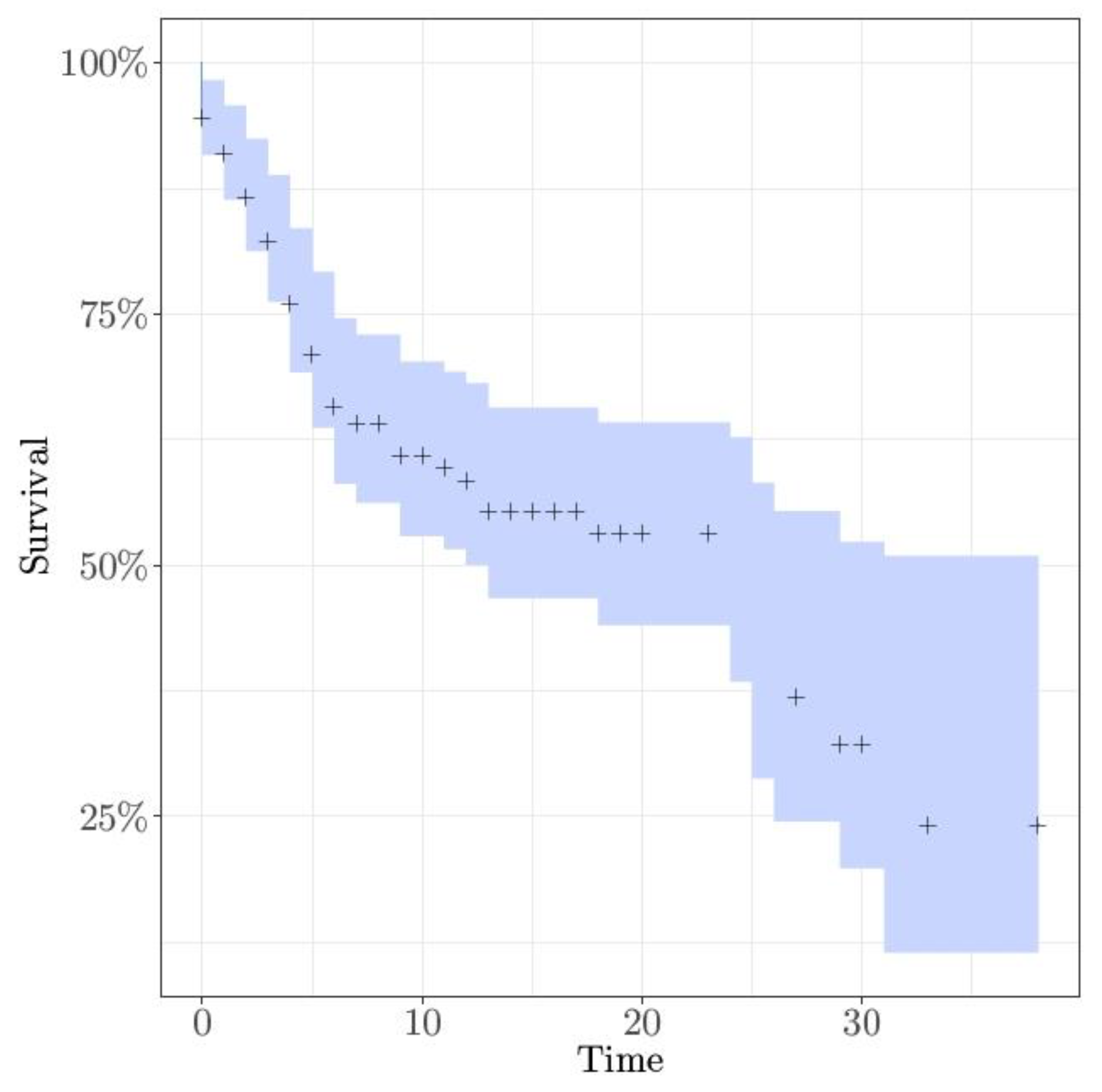
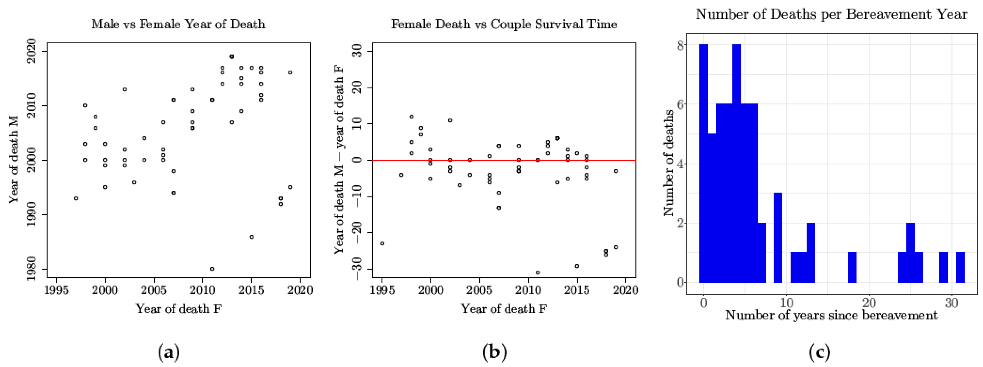
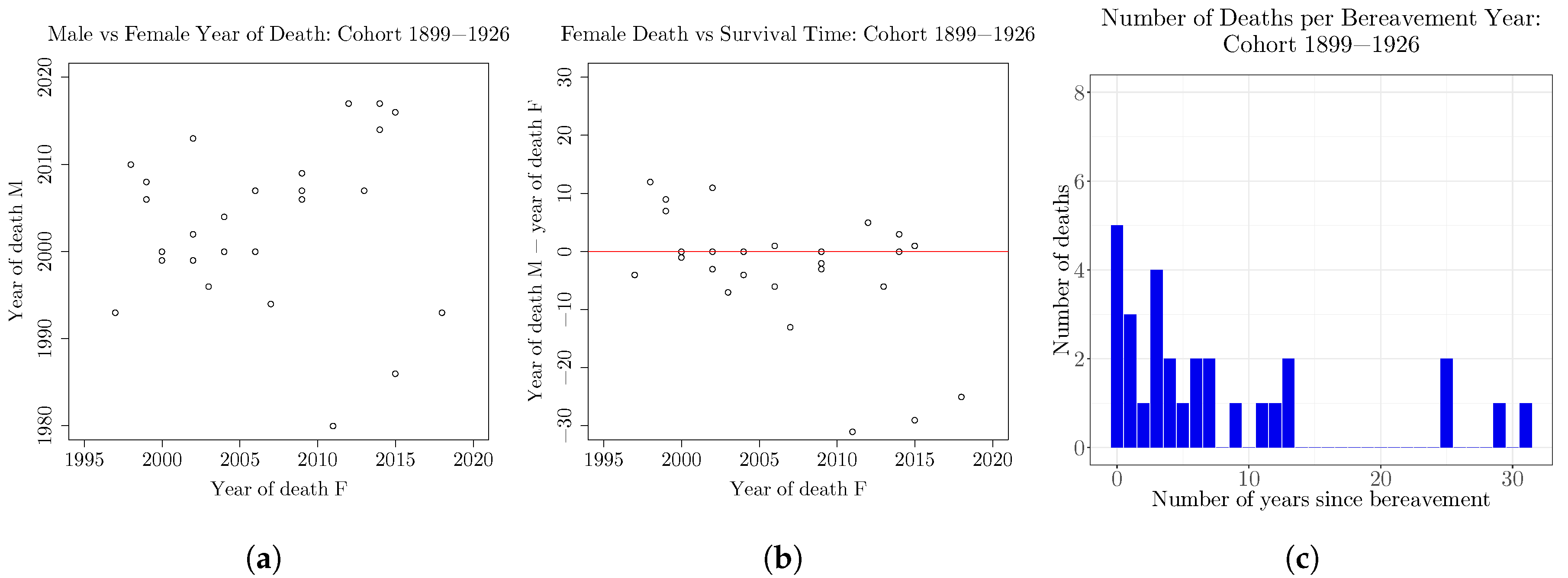
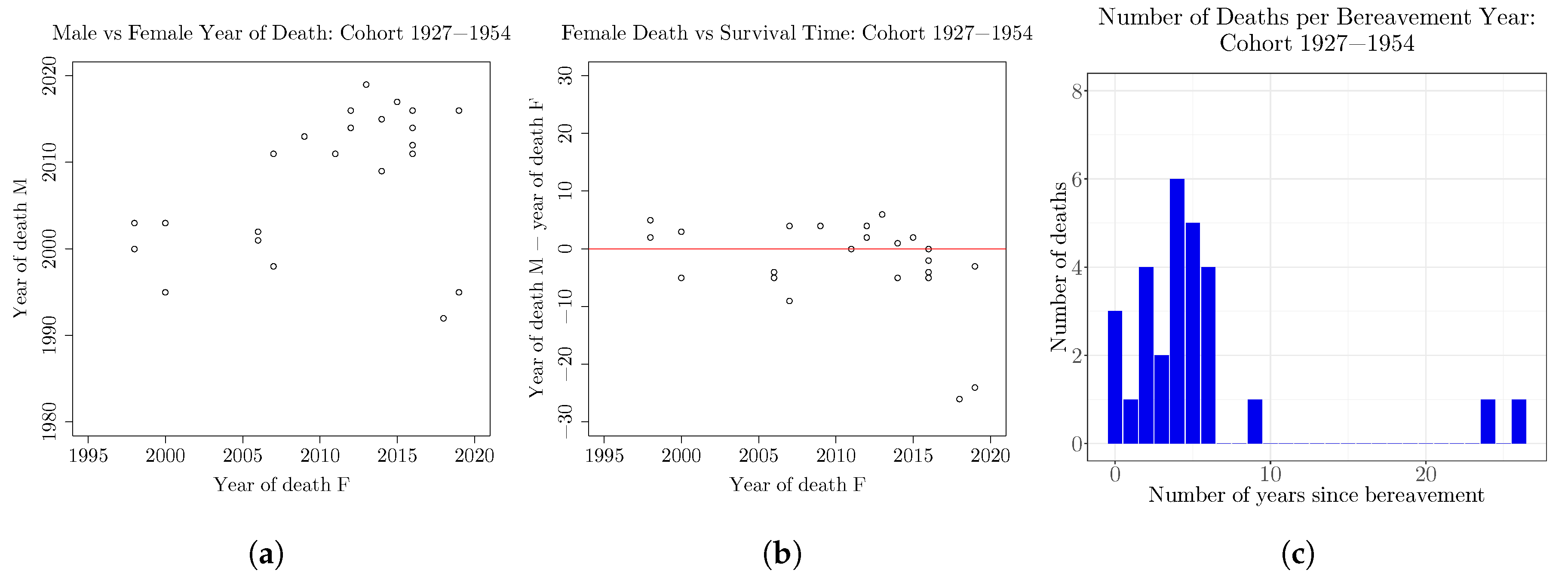
Table 1.
Comparison of indifference price with and without dependence assumption.
| Dependent Price | Independent Price | |
|---|---|---|
| 0.8199 | 1.2005 | |
| 0.6953 | 0.9291 | |
| 0.5376 | 0.5764 |
© 2020 by the authors. Licensee MDPI, Basel, Switzerland. This article is an open access article distributed under the terms and conditions of the Creative Commons Attribution (CC BY) license (http://creativecommons.org/licenses/by/4.0/).
Share and Cite
MDPI and ACS Style
Henshaw, K.; Constantinescu, C.; Menoukeu Pamen, O. Stochastic Mortality Modelling for Dependent Coupled Lives. Risks 2020, 8, 17. https://0-doi-org.brum.beds.ac.uk/10.3390/risks8010017
AMA Style
Henshaw K, Constantinescu C, Menoukeu Pamen O. Stochastic Mortality Modelling for Dependent Coupled Lives. Risks. 2020; 8(1):17. https://0-doi-org.brum.beds.ac.uk/10.3390/risks8010017
Chicago/Turabian StyleHenshaw, Kira, Corina Constantinescu, and Olivier Menoukeu Pamen. 2020. "Stochastic Mortality Modelling for Dependent Coupled Lives" Risks 8, no. 1: 17. https://0-doi-org.brum.beds.ac.uk/10.3390/risks8010017
Note that from the first issue of 2016, this journal uses article numbers instead of page numbers. See further details here.