A Poisson Autoregressive Model to Understand COVID-19 Contagion Dynamics


Department of Economics and Management, University of Pavia, 27100 Pavia, Italy
*
Author to whom correspondence should be addressed.
Risks 2020, 8(3), 77; https://0-doi-org.brum.beds.ac.uk/10.3390/risks8030077
Submission received: 9 June 2020
/
Revised: 27 June 2020
/
Accepted: 11 July 2020
/
Published: 16 July 2020
(This article belongs to the Special Issue Risks: Feature Papers 2020)
Abstract
:We present a statistical model which can be employed to understand the contagion dynamics of the COVID-19, which can heavily impact health, economics and finance. The model is a Poisson autoregression of the daily new observed cases, and can reveal whether contagion has a trend, and where is each country on that trend. Model results are exemplified from some observed series.
1. Motivation
The spread of the COVID-19 virus at the beginning of 2020 caught many countries and governments by surprise and unveiled a widespread lack of pandemic preparedness at the global and national level.
Currently, given the absence of a vaccine and the incomplete information about several aspects of contagion, such as the role of different risk factors, the dynamics of transmission and the role of asymptomatic transmission, governments operate under significant uncertainty. Against this background, data from countries where the virus has initially spread (notably China) are a precious source of information for the countries that are fighting against the virus. The more data becomes available, the more policies can be formulated with the backing of evidence as regards the “curve” and the “peak” of the contagion.
Early attempts to model the contagion curve of the COVID-19 include (Danon et al. 2020), which predicted that the outbreak would peak 126 to 147 days (around 4 months) after the start of person-to-person transmission in England and Wales, at a time in which the virus had been found in just 25 countries; and (Kucharski et al. 2020), which combines a stochastic transmission model with four datasets on cases of COVID-19 originated in Wuhan to estimate how transmission varied over time, and calculate the probability that newly introduced cases might generate outbreaks in other areas. In Imperial College COVID-19 Response Team (2020), researchers modified an individual-based simulation model developed to support pandemic influenza planning to explore scenarios for COVID-19 in Great Britain.
Particularly relevant studies for our work are Gu et al. (2020) and Giordano et al. (2020) which, while mathematically expressing the current practices in the modelling on the global spread of diseases, draw policy making suggestions. We follow the same line of research, combining mathematical rigour with attention to drawing results that can be useful for policy makers. Specifically, our contribution is a new statistical model for disease spread which, by taking dependence between daily contagion counts into account, can better capture the contagion curve dynamics and, thus, can draw further light on the understanding of its possible future path.
Our approach is connected to the exponential growth models employed in the SIR literature (Biggerstaff et al. 2014), to which we contribute by including an autoregressive component in the growth dynamics.
2. Methodology
We aim to build a monitoring model which can provide support to policy makers engaged in contrasting the spread of the COVID-19, and their economical consequences. To this aim, we propose a statistical model that can estimate when the peak of contagion is reached, so that preventive measures (such as mobility restrictions) can be applied and/or relaxed.
To be built the model requires, for each country (or region), the daily count of new infections. In the study of epidemics, it is usually assumed that infection counts follow an exponential growth, driven by the reproduction number R (see, e.g., Biggerstaff et al. 2014). The latter can be estimated by the ratio between the new cases arising in consecutive days: a short-term dependence. This procedure, however, may not be adequate: incubation time is quite variable among individuals and data occurrence and measurement is not uniform across different countries (and, sometimes, along time): these aspects induce a long-term dependence.
From the previous considerations, it follows that it would be ideal to model newly infected counts as a function of both a short-term and a long-term component. A model of this kind has been recently proposed by Agosto et al. (2016), in the context of financial contagion. We propose to adapt this model to the COVID-19 contagion.
Formally, resorting to the log-linear version of Poisson autoregression, introduced by Fokianos and Tjøstheim (2011), we assume that the statistical distribution of new cases at time (day) t, conditional on the information up to , is Poisson, with a log-linear autoregressive intensity, as follows:
where denotes the -field generated by , , , , . Note that the inclusion of , rather than , allows to deal with zero values.
In the model, is the intercept term, whereas and express the dependence of the expected number of new infections, , on the past counts of new infections. Specifically, the component represents the short-term dependence on the previous time point. The component represents a trend component, that is, the long-term dependence on all past values of the observed process. The inclusion of the component is analogous to moving from an ARCH (Engle 1982) to a GARCH (Engle and Bollerslev 1986) model in Gaussian processes, and allows to capture long memory effects. The advantage of a log-linear intensity specification, rather than the linear one known as integer-valued GARCH (see, e.g., Ferland et al. 2006), is that it allows for negative dependence. From an inferential viewpoint, Fokianos and Tjøstheim (2011) show that the model can be estimated by a maximum likelihood method.
3. Results
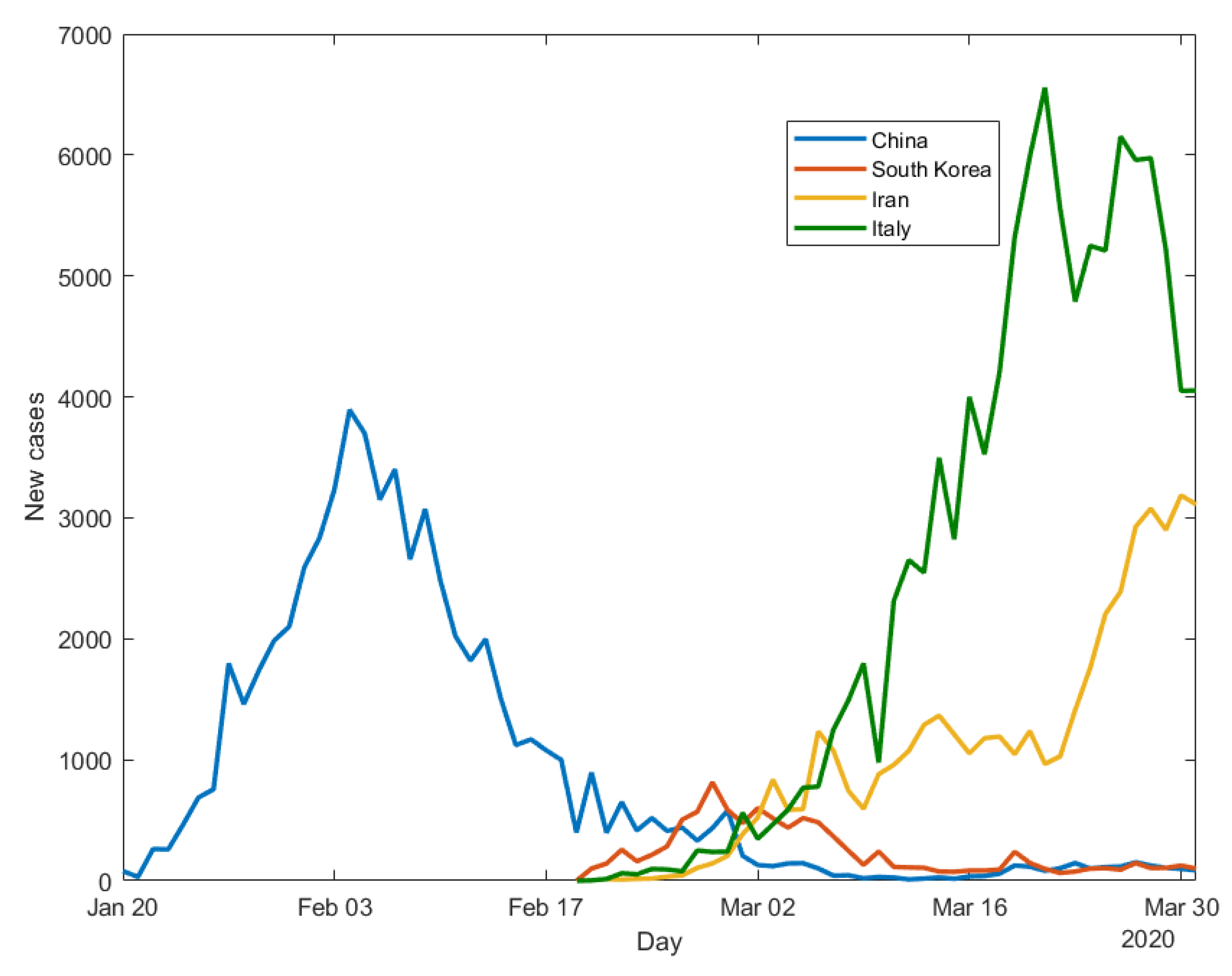
The model can be applied to any country, region, and in different time periods. We exemplify its usage, without loss of generality, using data available until 31 March 2020. The data source is the daily World Health Organisation reports (see World Health Organisation 2020), from which we have extracted the “Total confirmed new cases”. Figure 1 presents the observed evolution of the daily new cases of infection: for China (starting from 20 January), Iran, South Korea and Italy (starting from 21 February). We choose to consider data until the end of March (Figure 1) and make predictions for the beginning of April because at that time contagion counts in the analysed countries were still high and predictions challenging. Being the count response variable a Poisson, its variance depends on the number of observed counts, a number which has been declining in the considered countries, from April onwards, when not before.
Figure 1 shows that, as of 31 March 2020, COVID-19 contagion in China has completed a full cycle, with an upward trend, a peak, and a downward trend. South Korea seems to have had a similar situation, with a smaller intensity. Italy has followed a similar path, with a larger intensity. The contagion dynamics in Iran is more difficult to interpret, and is still quite erratic.
The application of our model can better qualify these conclusions. The estimated model parameters for China, using all data available until 31 March, are shown in Table 1.
Table 1 shows that all estimated autoregressive coefficients are significant, confirming the presence of both a short-term dependence and a long-term trend. From an interpretational viewpoint, the estimate of shows that, if the expectation of new cases for yesterday was close to 0, 100 new cases observed yesterday generate about 40 new expected cases today. According to the value estimated for , an expectation of 100 new cases for yesterday generates instead about 2 new expected cases today, if no cases were observed yesterday.
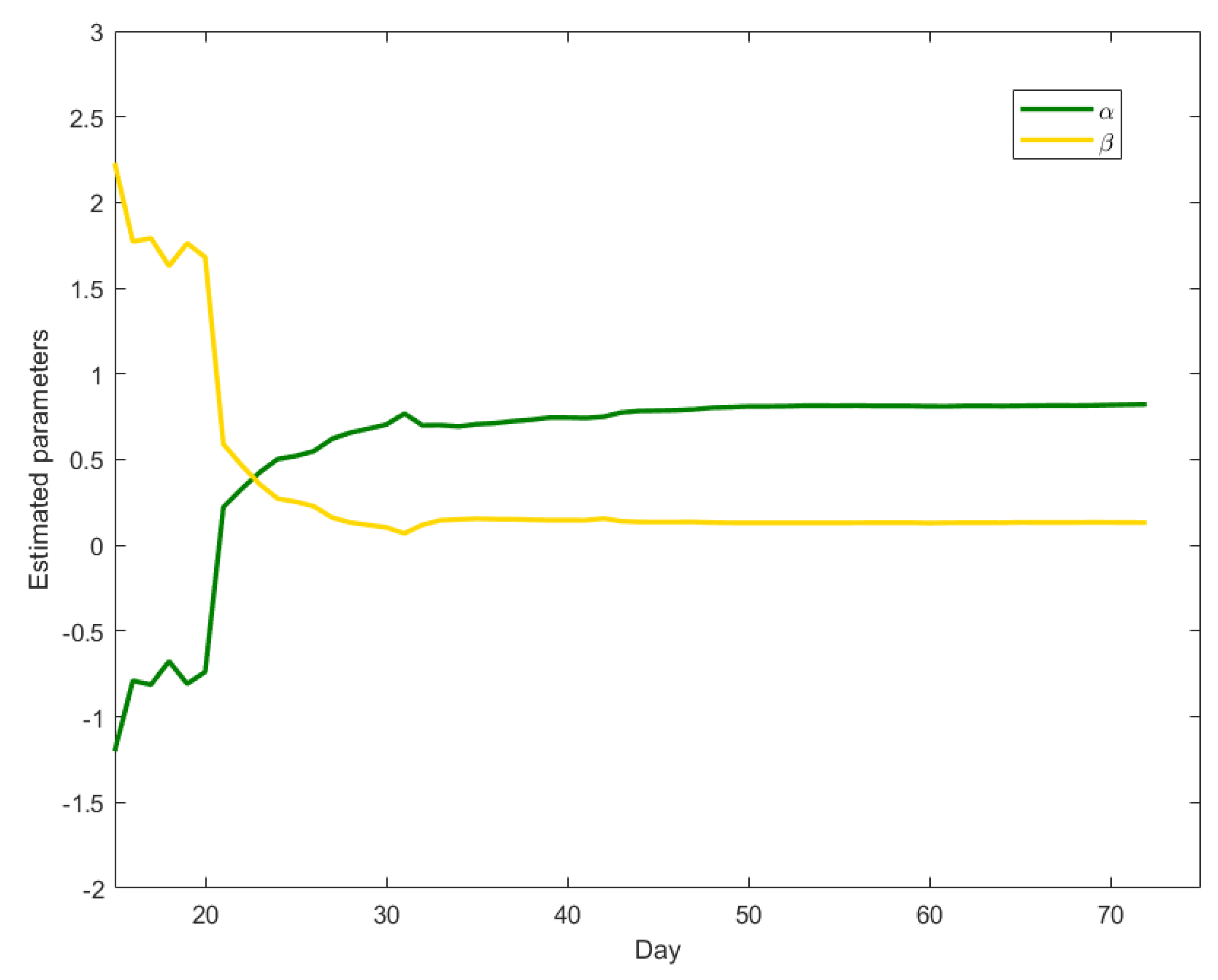
With the aim of better interpreting the time series of the other countries, which on 31 March seem not to have completed their contagion cycle yet, we repeatedly fit the model to the Chinese data, using increasing amounts of data, in a retrospective way. More precisely, we first fit the model on the first 15 counts from China (a minimal requirement for statistical consistency of the results), then on the first 16, and so on. For each fit we plot the estimated and parameters in Figure 2.
Figure 2 shows that, until February 11th (the 23rd day reported) is greater than , indicating the presence of a still increasing trend (the component) that absorbs the short-term component. After that time, downward trend data is accumulated, starts decreasing and increasing. The results approximate the values in Table 1 around 20 February: after this date the estimated parameters become stable, as the difference between subsequent estimates becomes lower than .
What obtained from the Chinese data suggests to use the PAR model to assess at which stage the contagion cycle is in the other countries. We thus estimate the model parameters for the other three countries, using the data available until 31 March. Our results show that, for Iran, on that date the parameter prevails, with an estimated value equal to , indicating a process mainly driven by a short-term dependence on the previous time points. However, further analyses reveal that the parameters estimated for Iran are very unstable. The estimated parameter for South Korea is not significant, indicating absence of a trend effect on the daily counts, consistently with what observed in Figure 1. For Italy, instead, is about , higher than , similarly to China but with a lower difference between the two parameters, indicating that, at the end of March, the trend component is weakening.
To conclude, we believe that our model can constitute a useful statistical tool for decision makers: in each country, once a minimal series of data is collected (we suggest 15 days) the values of and can be monitored along time, to reveal at which stage the contagion dynamics is: well beyond the peak (as in China and South Korea); close to or right after the peak (as Italy on 31 March); or in a situation that could indicate that the peak has been reached, but which needs more data to be understood (as Iran at the end of March).
The full reproducibility of our model can easily extend its application to more countries and time periods as data becomes available.
To better understand the advantages of our proposed specification and, at the same time, to show its possible improvement, we now compare it with two alternative models, one simpler and one more complex.
The first one is a classic exponential growth model, that is a regression of the number of daily new cases on the time, expressed as days since the outbreak:
The second alternative model we consider is a PARX model Agosto et al. (2016), that is a Poisson autoregressive model with a covariate. As a covariate we use time: the number of days since the outbreak, as in the classical exponential model. Thus, we extend the PAR model as follows:
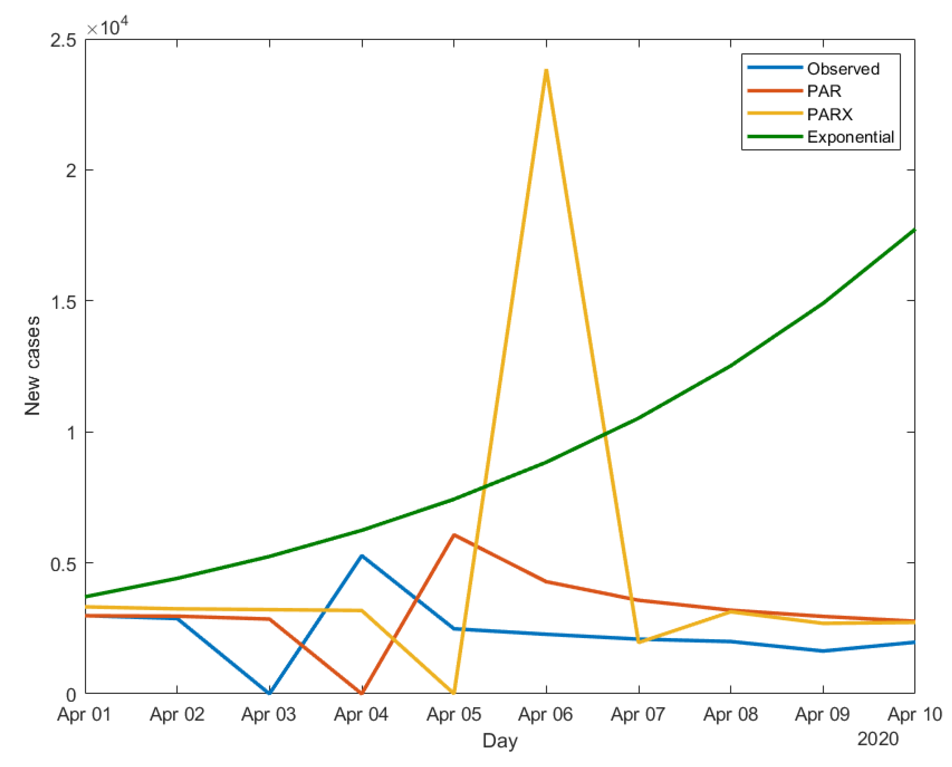
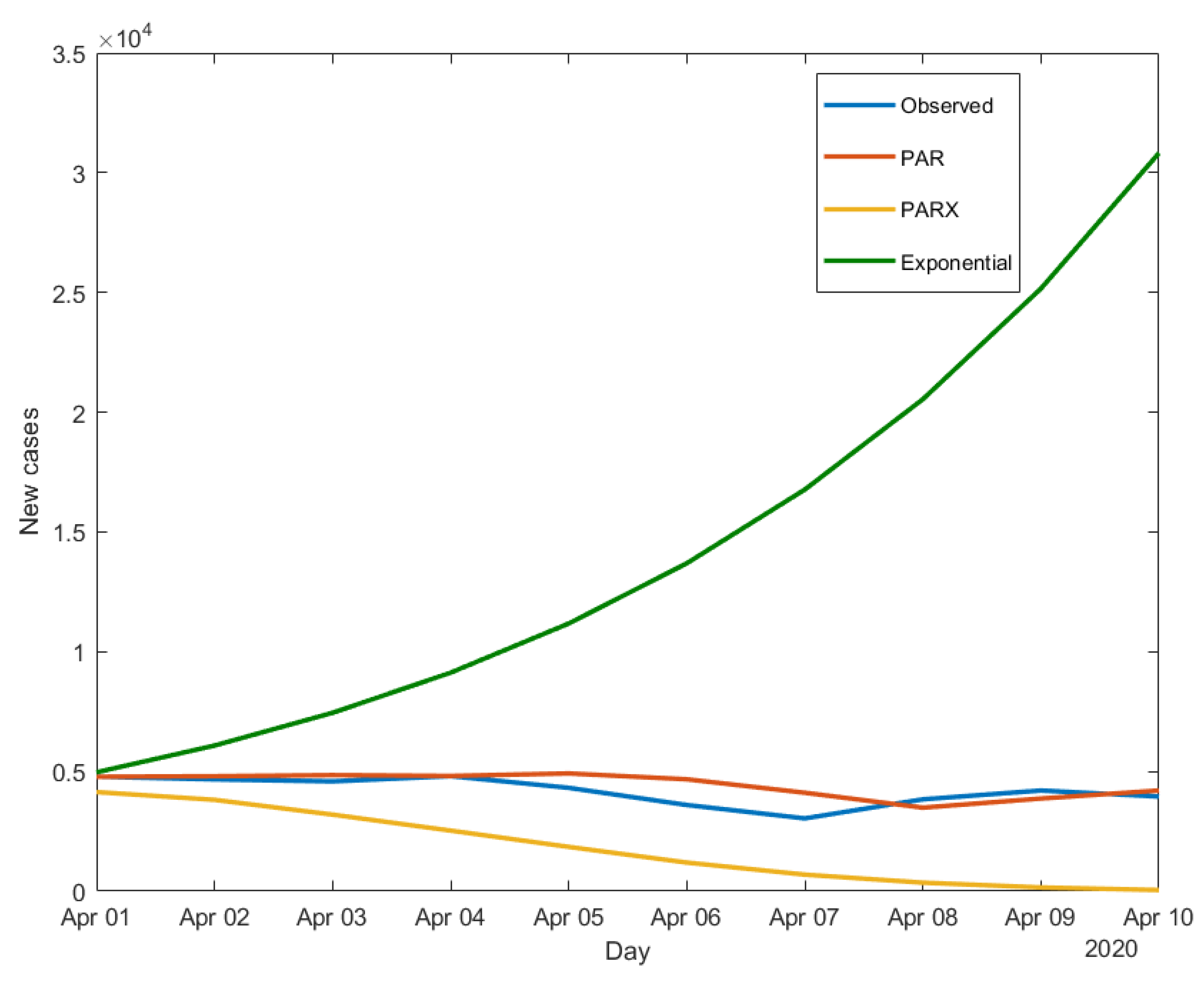
We now apply the three models-estimated using data until the end of March - to make 10-day ahead predictions of the daily new cases. The results obtained for South Korea, Iran and Italy are shown in Figure 3, Figure 4 and Figure 5.
Figure 3, Figure 4 and Figure 5 all show the limits of the exponential model, which, being a “static” model, cannot capture time variations in the contagion dynamics, differently from both the PAR and the PARX. The latter, being dynamic models, can better adapt to disease count variations, without the need to often adjust the estimates and find a saturation point, as it would be the case for the exponential model.
To compare the models in terms of out-of-sample predictive performance, in Table 2 we report the value of Root Mean Squared Error (RMSE) and Mean Percentage error (MPE) for the three specifications.
The results in Table 2 show that the PAR model always outperforms the other two, except in the case of South Korea, for which the preferable specification turns out to be Poisson autoregression including the time since outbreak as a covariate. This finding is consistent with what observed in Figure 3, Figure 4 and Figure 5 and confirms the superiority of Poisson autoregressive models over the exponential growth model. This advantage explains the potential impact of our proposal, which is successfully implemented and weekly updated in the infographic website of the Center for European Policy Studies1.
Author Contributions
All authors have read and agreed to the published version of the manuscript.
Funding
This research received no external funding.
Acknowledgments
The work of the Authors is receiving support from the European Union’s Horizon 2020 training and innovation programme “FIN-TECH”, under the grant agreement No. 825215 (Topic ICT-35-2018, Type of actions: CSA). The paper is the result of the joint collaboration between the two authors.
Conflicts of Interest
The authors declare no conflict of interest.
References
- Agosto, Arianna, Giuseppe Cavaliere, Dennis Kristensen, and Anders Rahbek. 2016. Modeling Corporate Defaults: Poisson Autoregressions with Exogenous Covariates (PARX). Journal of Empirical Finance 38: 640–63. [Google Scholar] [CrossRef] [Green Version]
- Biggerstaff, Matthew, Simon Cauchemez, Carrie Reed, Manoj Gambhir, and Lyn Finelli. 2014. Estimates of the reproduction number for seasonal, pandemic, and zoonotic influenza: A systematic review of the literature. BMC Infectious Diseases 14: 480. [Google Scholar] [CrossRef] [PubMed] [Green Version]
- Danon, Leon, Ellen Brooks-Pollock, Mick Bailey, and Matt J. Keeling. 2020. A Spatial Model of CoVID-19 Transmission in England and Wales: Early Spread and Peak Timing. Available online: https://www.medrxiv.org/content/10.1101/2020.02.12.20022566v1 (accessed on 30 April 2020).
- Engle, Robert F. 1982. Autoregressive Conditional Heteroscedasticity with Estimates of the Variance of U. K. Inflation. Econometrica: Journal of the Econometric Society 50: 987–1008. [Google Scholar] [CrossRef]
- Engle, Robert F., and Tim Bollerslev. 1986. Modelling the persistence of conditional variances. Econometric Reviews 5: 1–50. [Google Scholar] [CrossRef]
- Ferland, René, Alain Latour, and Driss Oraichi. 2006. Integer-valued GARCH processes. Journal of Time Series Analysis 27: 923–42. [Google Scholar] [CrossRef]
- Fokianos, Konstantinos, and Dag Tjøstheim. 2011. Log-linear Poisson autoregression. Journal of Multivariate Analysis 102: 563–78. [Google Scholar] [CrossRef]
- Giordano, Giulia, Franco Blanchini, Raffaele Bruno, Patrizio Colaneri, Alessandro Di Filippo, Angela Di Matteo, and Marta Colaneri. 2020. Modelling the COVID-19 epidemic and implementation of population wide interventions in Italy. Nature Medicine 26: 855–60. [Google Scholar] [CrossRef] [PubMed]
- Gu, Chenlin, Wei Jiang, Tianyuan Zhao, and Ban Zheng. 2020. Mathematical Recommendations to Fight against COVID-19. Available online: https://papers.ssrn.com/sol3/papers.cfm?abstract_id=3551006 (accessed on 30 April 2020).
- Imperial College COVID-19 Response Team. 2020. Impact of Non-Pharmaceutical Interventions (NPIs) to Reduce COVID19 Mortality and Healthcare Demand. Available online: https://www.imperial.ac.uk/media/imperial-college/medicine/sph/ide/gida-fellowships/Imperial-College-COVID19-NPI-modelling-16-03-2020.pdf (accessed on 30 April 2020).
- Kucharski, Adam J., Timothy W. Russell, Charlie Diamond, Yang Liu, John Edmunds, Sebastian Funk, Rosalind M. Eggo, Fiona Sun, Mark Jit, James D Munday, and et al. 2020. Early Dynamics of Transmission and Control of COVID-19: A Mathematical Modelling Study. Centre for Mathematical Modelling of Infectious Diseases COVID-19 Working Group. Available online: http://docplayer.fr/11284694-Tables-de-probabilites-et-statistique.html (accessed on 30 April 2020).
- World Health Organisation. 2020. Novel Coronavirus (2019-nCoV) Situation Reports. pp. 1–49. Available online: https://apps.who.int/iris/bitstream/handle/10665/330762/nCoVsitrep23Jan2020-eng.pdf (accessed on 30 April 2020).
| 1 |
Figure 1.
Observed infection counts.

Figure 2.
Evolution of the and parameters for Chinese daily infection counts.

Figure 3.
Daily infection counts in South Korea: observed and predicted values.

Figure 4.
Daily infection counts in Iran: observed and predicted values.

Figure 5.
Daily infection counts in Italy: observed and predicted values.


Table 1.
Model estimates for China, with standard errors and p-values.
| Parameter | Estimate | Std Error (p-Value) |
|---|---|---|
| 0.337 | 0.247 (0.177) | |
| 0.823 | 0.069 (0.000) | |
| 0.133 | 0.062 (0.016) |
Table 2.
Out-of-sample error measures.
| South Korea | Iran | Italy | ||||
|---|---|---|---|---|---|---|
| Model | RMSE | MPE | RMSE | MPE | RMSE | MPE |
| PAR | 19.48 | −31.04% | 2426.2 | −0.29% | 551.79 | −7.69% |
| PARX | 14.18 | −14.44% | 6996.1 | −49.33% | 2633.4 | 59.63% |
| Exponential | 47.28 | −103.1% | 8399.5 | −156.30% | 13,441 | −269.17% |
© 2020 by the authors. Licensee MDPI, Basel, Switzerland. This article is an open access article distributed under the terms and conditions of the Creative Commons Attribution (CC BY) license (http://creativecommons.org/licenses/by/4.0/).
Share and Cite
MDPI and ACS Style
Agosto, A.; Giudici, P. A Poisson Autoregressive Model to Understand COVID-19 Contagion Dynamics. Risks 2020, 8, 77. https://0-doi-org.brum.beds.ac.uk/10.3390/risks8030077
AMA Style
Agosto A, Giudici P. A Poisson Autoregressive Model to Understand COVID-19 Contagion Dynamics. Risks. 2020; 8(3):77. https://0-doi-org.brum.beds.ac.uk/10.3390/risks8030077
Chicago/Turabian StyleAgosto, Arianna, and Paolo Giudici. 2020. "A Poisson Autoregressive Model to Understand COVID-19 Contagion Dynamics" Risks 8, no. 3: 77. https://0-doi-org.brum.beds.ac.uk/10.3390/risks8030077
Note that from the first issue of 2016, this journal uses article numbers instead of page numbers. See further details here.