Nagging Predictors

Abstract

We define the nagging predictor, which, instead of using bootstrapping to produce a series of i.i.d. predictors, exploits the randomness of neural network calibrations to provide a more stable and accurate predictor than is available from a single neural network run. Convergence results for the family of Tweedie’s compound Poisson models, which are usually used for general insurance pricing, are provided. In the context of a French motor third-party liability insurance example, the nagging predictor achieves stability at portfolio level after about 20 runs. At an insurance policy level, we show that for some policies up to 400 neural network runs are required to achieve stability. Since working with 400 neural networks is impractical, we calibrate two meta models to the nagging predictor, one unweighted, and one using the coefficient of variation of the nagging predictor as a weight, finding that these latter meta networks can approximate the nagging predictor well, only with a small loss of accuracy.

1. Introduction

Aggregating is a statistical technique that helps to reduce noise and uncertainty in predictors. Typically, it is applied to an i.i.d. sequence of predictors and it is justified theoretically using the law of large numbers. In many practical applications one is not in the comfortable situation of having an i.i.d. sequence of predictors to which aggregating could be applied. For this reason, Breiman (1996) combined bootstrapping and aggregating, called bagging, bootstrapping being used to generate a sequence of randomized predictors and then aggregating them to receive an averaged bootstrap predictor. The title of this paper has been inspired by Breiman (1996), in other words, it is not meant in the sense of grumbling or the like, but we are going to combine networks and aggregating to receive the nagging predictor. Thereby, we benefit from the fact that typically neural network regression models have infinitely many equally good predictors which are determined by gradient descent algorithms. These equally good predictors depend on the (random) starting point of the gradient descent algorithm, thus, starting the algorithm in i.i.d. seeds for different runs results in an infinite sequence of (equally good) neural network predictors. Moreover, other common neural network training techniques may even lead to more randomness in neural network results, for example, dropout, which relies on randomly setting parts of the network to zero during training to improve performance at test time, see Srivastava et al. (2014) for more details, or the random selection of data to implement stochastic or mini-batch gradient descent methods. On the one hand, this creates difficulties for using neural network models within an insurance pricing context, since the predictive performance of the models measured at portfolio level will vary with each run and the predictions for individual policies will vary even more, leading to uncertainty about the prices that should ultimately be charged to individuals. On the other hand, having multiple network predictors puts us in the same situation as Breiman (1996) after having received the bootstrap samples, and we can aggregate them, leading to more stable results and enhanced predictive performance. In this paper, we explore statistical properties of nagging predictors at a portfolio and at a policy level, in the context of insurance pricing.

We give a short review of related literature. Aggregation of predictors is also known as ensembling. Dietterich (2000a, 2000b) discusses ensembling within various machine learning methods such as decision trees and neural networks. As stated in Dietterich (2000b), successful ensembling crucially relies on the fact that one has to be able to construct multiple suitable predictors. This is usually achieved by injecting randomness either into the data or into the fitting algorithm. In essence, this is what we do in this study, however, our main objective is to reduce randomness (in the results of the fitting algorithms) because, from a practical perspective, we need to have uniqueness in insurance pricing, in particular, we prove rates of convergence at which the random element can be diminished. Zhou (2012) and Zhou et al. (2002) study optimal ensembling of multiple predictors. Their proposal leads to a quadratic optimization problem that can be solved with the method of Lagrange. This is related to our task below of finding an optimal meta model using individual uncertainties which we discuss in Section 5.8, below. Related empirical studies on financial data are given in Di Persio and Honchar (2016), du Jardin (2016) and Wang et al. (2011). These studies conclude that ensembling is very beneficial to improve predictive performance which, indeed, is also one of our main findings.

Organization of manuscript. In the next section we introduce the framework of neural network regression models, and we discuss their calibration within Tweedie’s compound Poisson models. In Section 3 we give the theoretical foundation of aggregating predictors, in particular, we prove that aggregating leads to more stability in prediction in terms of a central limit theorem. In Section 4 we implement aggregation within the framework of neural network predictors providing the nagging predictor. In Section 5 we empirically prove the effectiveness of nagging predictors based on a French car insurance data set. Since nagging predictors involve simultaneously dealing with multiple networks, we provide a more practical meta network that approximates the nagging predictor at a minimal loss of accuracy.

2. Feed-Forward Neural Network Regression Models

These days neural networks are state-of-the-art for performing complex regression and classification tasks, particularly on unstructured data such as images or text. For a general introduction to neural networks we refer to LeCun et al. (2015), Goodfellow et al. (2016) and the references therein. In the present work, we follow the terminology and notation of Wüthrich (2019). We design feed-forward neural network regression models, referred to in short as networks, to predict insurance claims. In the spirit of Wüthrich (2019), we understand these networks as extensions of generalized linear models (GLMs), the latter being introduced by Nelder and Wedderburn (1972).

2.1. Generic Definition of Feed-Forward Neural Networks

Assume we have independent observations $(Y_i,{\mathit{x}}_i,v_i)$, $i=1,\dots ,n$; the variables $Y_i$ describe the responses (here: insurance claims), ${\mathit{x}}_i\in \mathcal{X}\subset {\mathbb{R}}^{q_0}$ describe the real-valued feature information (also known as covariates, explanatory variables, independent variables or predictors), and $v_i>0$ are known exposures. The main goal is to find a regression functional $\mu (·)$ that appropriately describes the expected insurance claims $\mathbb{E}\left[Y_i\right]$ as a function of the feature information ${\mathit{x}}_i$, i.e.,

$$\mathcal{X}\to \mathbb{R},{\mathit{x}}_i\mapsto \mu \left({\mathit{x}}_i\right)=\mathbb{E}\left[Y_i\right].$$

Since, typically, the true regression function $\mu$ is unknown we approximate it by a network regression function. Under a suitable link function choice $g(·)$, we assume that $\mathbb{E}\left[Y_i\right]$ can be described by the following network of depth $d\in \mathbb{N}$

$${\mathit{x}}_i\mapsto g\left(\mathbb{E}\left[Y_i\right]\right)=〈{\mathit{\beta }}^{(d+1)},\left({\mathit{z}}^{\left(d\right)}\circ \cdots \circ {\mathit{z}}^{\left(1\right)}\right)\left({\mathit{x}}_i\right)〉,$$

(1)

where $\langle ·,·\rangle$ is the scalar product in Euclidean space ${\mathbb{R}}^{q_d+1}$, the operation ○ gives a composition of hidden network layers ${\mathit{z}}^{\left(m\right)}$, $1\le m\le d$, of dimensions $q_m+1\in \mathbb{N}$, and ${\mathit{\beta }}^{(d+1)}\in {\mathbb{R}}^{q_d+1}$ is the readout parameter. For a given non-linear activation function $\varphi :\mathbb{R}\to \mathbb{R}$, the m-th hidden network layer is a mapping

$${\mathit{z}}^{\left(m\right)}:\left\{1\right\}\times {\mathbb{R}}^{q_{m-1}}\to \left\{1\right\}\times {\mathbb{R}}^{q_m},\mathit{x}\mapsto {\mathit{z}}^{\left(m\right)}\left(\mathit{x}\right)={\left(1,z_1^{\left(m\right)}\left(\mathit{x}\right),\dots ,z_{q_m}^{\left(m\right)}\left(\mathit{x}\right)\right)}^{\top },$$

with hidden neurons $z_j^{\left(m\right)}(·)$, $1\le j\le q_m$, being described by ridge functions

$$\mathit{x}\mapsto z_j^{\left(m\right)}\left(\mathit{z}\right)=\varphi 〈{\mathit{\beta }}_j^{\left(m\right)},\mathit{x}〉,$$

for network parameters ${\mathit{\beta }}_j^{\left(m\right)}\in {\mathbb{R}}^{q_{m-1}+1}$. This network regression function has a network parameter $\mathit{\beta }=({\mathit{\beta }}_1^{\left(1\right)},\dots ,{\mathit{\beta }}_{q_d}^{\left(q\right)},{\mathit{\beta }}^{(d+1)})\in {\mathbb{R}}^r$ of dimension $r={\sum }_{m=1}^{d+1}(q_{m-1}+1)q_m$.

Based on so-called universality theorems, see, for example, Cybenko (1989) and Hornik et al. (1989), we know that networks are very flexible and can approximate any continuous and compactly supported regression function arbitrarily well if one allows for a sufficiently complex network architecture. In practical applications this means that one has to choose sufficiently many hidden layers with sufficiently many hidden neurons to be assured of adequate approximation capacity, and then one can work with this network architecture as a replacement of the unknown regression function. This complex network is calibrated to (learning) data using the gradient descent algorithm. To prevent the network from over-fitting to the learning data, one exercises early stopping of this calibration algorithm by applying a given stopping rule. This early stopping of the algorithm before convergence typically implies that one cannot expect to receive a “unique best” model, in fact, the early stopped calibration depends on the starting point of the gradient descent algorithm and, usually, since each run has a different starting point, one receives a different solution each time early-stopped gradient descent is run. As described in Section 3.3.1 of Wüthrich (2019), this exactly results in the problem of having infinitely many equally good models for a fixed stopping rule, and it is not clear which particular solution should be chosen, say, for insurance pricing. This is the main point on which we elaborate in this work, and we come back to this discussion after Equation (7), below.

2.2. Tweedie’s Compound Poisson Model

We assume that the response $Y_i$ in Equation (1) belongs to the family of Tweedie’s compound Poisson (CP) models, see Tweedie (1984), having a density of the form

$$Y_i\sim f(y;{\theta }_i,v_i/\phi ,p)=exp\left\{\frac{y{\theta }_i-{\kappa }_p\left({\theta }_i\right)}{\phi /v_i}+a_p(y;v_i/\phi )\right\},$$

(2)

with $p\in [1,2]$ being the power variance (hyper-)parameter, and

$$\begin{array}{cc}{v}_i>0& \mathrm{is}\mathrm{a}\mathrm{given}\mathrm{exposure}(\mathrm{weight},\mathrm{volume}),\hfill \\ \phi >0& \mathrm{is}\mathrm{the}\mathrm{dispersion}\mathrm{parameter},\hfill \\ {\theta }_i\in {\mathbf{\Theta }}_p& \mathrm{is}\mathrm{the}\mathrm{canonical}\mathrm{parameter}\mathrm{in}\mathrm{the}\mathrm{effective}\mathrm{domain}{\mathbf{\Theta }}_p,\hfill \\ {\kappa }_p:{\mathbf{\Theta }}_p\to \mathbb{R}& \mathrm{is}\mathrm{a}\mathrm{cumulant}\mathrm{function}\mathrm{of}\mathrm{the}\mathrm{form}\mathrm{Equation}(3),\mathrm{below},\hfill \\ a_p(·;·)& \mathrm{is}\mathrm{the}\mathrm{normalization},\mathrm{not}\mathrm{depending}\mathrm{on}\mathrm{the}\mathrm{canonical}\mathrm{parameter}{\theta }_i.\hfill \end{array}$$

Tweedie’s CP models belong to the exponential dispersion family (EDF), the latter being more general because it allows for more general cumulant functions $\kappa$, we refer to Jørgensen (1986, 1987). We focus here on Tweedie’s CP family and not on the entire EDF because for certain calculations we need explicit properties of cumulant functions. However, similar results can be derived for other members of the EDF. We mention that the effective domain ${\mathbf{\Theta }}_p\subset \mathbb{R}$ is a convex set, and that the cumulant function ${\kappa }_p$ is smooth and strictly convex in the interior of the effective domain, having the following explicit form

$${\kappa }_p\left(\theta \right)=\left\{\begin{array}{cc}exp\left(\theta \right)\hfill & \mathrm{for}p=1,\hfill \\ \frac{1}{2-p}{((1-p)\theta )}^{\frac{2-p}{1-p}}\hfill & \mathrm{for}p\in (1,2),\hfill \\ -log(-\theta )\hfill & \mathrm{for}p=2.\hfill \end{array}\right.$$

(3)

$p=1$ is the Poisson model (with $\phi =1$), $p=2$ is the gamma model, and for $p\in (1,2)$ we receive compound Poisson models with i.i.d. gamma claim sizes having shape parameter $\gamma =(2-p)/(p-1)\in (0,\infty )$, see Jørgensen and de Souza (1994) and Smyth and Jørgensen (2002). The first two moments are given by

$${\mu }_i\stackrel{\mathrm{def}.}{=}\mathbb{E}\left[Y_i\right]={\kappa }_p^{\prime }\left({\theta }_i\right)\mathrm{and}\mathrm{Var}\left(Y_i\right)=\frac{\phi }{v_i}{\kappa }_p^{″}\left({\theta }_i\right)=\frac{\phi }{v_i}{V}_p\left({\mu }_i\right),$$

(4)

with power variance function $V_p\left(\mu \right)={\mu }^p$ for $p\in [1,2]$.

Remark 1.

In this paper we work under Tweedie’s CP models characterized by cumulant functions of the form Equation (3) because we need certain (explicit) properties of ${\kappa }_p$ in the proofs of the statements below. For regression modeling one usually starts from a bigger class of models, namely, the EDF, which only requires that the cumulant function is smooth and strictly convex on the interior of the corresponding effective domainΘ, see Jørgensen (1986, 1987). A sub-family of the EDF is the so-called Tweedie’s distributions which have a cumulant function that allows for a power mean-variance relationship Equation (4) for any $p\in \mathbb{R}\setminus (0,1)$, see Table 1 in Jørgensen (1987), for instance, $p=0$ is the Gaussian model, $p=1$ is the Poisson model, $p=2$ is the gamma model and $p=3$ is the inverse Gaussian model. As mentioned, the models generated by cumulant function Equation (3) cover the interval $(1,2)$ and correspond to compound Poisson models with i.i.d. gamma claim size, we also refer to Delong et al. (2020).

Relating Equation (3) to network regression function Equation (1) implies that we aim at modeling the canonical parameter ${\theta }_i$ of policy i by

$${\mathit{x}}_i\mapsto {\theta }_i=\theta \left({\mathit{x}}_i\right)={\left({\kappa }_p^{\prime }\right)}^{-1}\left(\mu \left({\mathit{x}}_i\right)\right)={\left({\kappa }_p^{\prime }\right)}^{-1}\left(g^{-1}\left(〈{\mathit{\beta }}^{(d+1)},\left({\mathit{z}}^{\left(d\right)}\circ \cdots \circ {\mathit{z}}^{\left(1\right)}\right)\left({\mathit{x}}_i\right)〉\right)\right),$$

(5)

and ${\left({\kappa }_p^{\prime }\right)}^{-1}$ is the canonical link, in contrast to the general link function g. If we choose the canonical link for g then ${\left({\kappa }_p^{\prime }\right)}^{-1}\circ g^{-1}$ provides the identity function in Equation (5). Network parameter $\mathit{\beta }\in {\mathbb{R}}^r$ is estimated with maximum likelihood estimation (MLE). This is achieved either by maximizing the log-likelihood function or by minimizing the corresponding deviance loss function. We use the framework of the deviance loss function here because it is more closely related to the philosophy of minimizing an objective function in gradient descent methods. The average deviance loss for independent random variables $Y_i$ is under Tweedie’s CP model assumption given by

$$\begin{array}{ccc}\mathcal{L}(\mathcal{D};\mathit{\beta })\hfill & =\hfill & \frac{2}{n}{\sum }_{i=1}^n\frac{v_i}{\phi }\left[Y_i{\left({\kappa }_p^{\prime }\right)}^{-1}\left(Y_i\right)-{\kappa }_p\left({\left({\kappa }_p^{\prime }\right)}^{-1}\left(Y_i\right)\right)-Y_i{\theta }_i+{\kappa }_p\left({\theta }_i\right)\right]\hfill \\ & =\hfill & \frac{2}{n}{\sum }_{i=1}^n\frac{v_i}{\phi }\left[Y_i{\left({\kappa }_p^{\prime }\right)}^{-1}\left(Y_i\right)-{\kappa }_p\left({\left({\kappa }_p^{\prime }\right)}^{-1}\left(Y_i\right)\right)-Y_i{\left({\kappa }_p^{\prime }\right)}^{-1}\left({\mu }_i\right)+{\kappa }_p\left({\left({\kappa }_p^{\prime }\right)}^{-1}\left({\mu }_i\right)\right)\right],\hfill \end{array}$$

(6)

for given data $\mathcal{D}=\{(Y_i,{\mathit{x}}_i,v_i);i=1,\dots ,n\}$. The canonical parameter is given by ${\theta }_i=\theta ({\mathit{x}}_i,\mathit{\beta })$ if we understand it as a function defined through Equation (5). Naturally we have for any mean parameter ${\mu }_i$ of any policy i

$$\delta (Y_i,{\mu }_i)\stackrel{\mathrm{def}.}{=}\frac{2v_i}{\phi }\left[Y_i{\left({\kappa }_p^{\prime }\right)}^{-1}\left(Y_i\right)-{\kappa }_p\left({\left({\kappa }_p^{\prime }\right)}^{-1}\left(Y_i\right)\right)-Y_i{\left({\kappa }_p^{\prime }\right)}^{-1}\left({\mu }_i\right)+{\kappa }_p\left({\left({\kappa }_p^{\prime }\right)}^{-1}\left({\mu }_i\right)\right)\right]\ge 0,$$

(7)

because these terms subtract twice the log-likelihood of the ${\mu }_i$-parametrized model from its saturated counterpart. $\delta (Y_i,{\mu }_i)$ is called the unit deviance of $Y_i$ w.r.t. mean parameter ${\mu }_i$.

The gradient descent algorithm now tries to make the objective function $\mathcal{L}(\mathcal{D};\mathit{\beta })$ small through optimizing network parameter $\mathit{\beta }$. This is done globally, i.e., simultaneously on the entire portfolio $i=1,\dots ,n$. Naturally, two different parameters ${\mathit{\beta }}^{\left(1\right)}\ne {\mathit{\beta }}^{\left(2\right)}$ with $\mathcal{L}(\mathcal{D};{\mathit{\beta }}^{\left(1\right)})=\mathcal{L}(\mathcal{D};{\mathit{\beta }}^{\left(2\right)})$ may provide very different models on an individual policy level i. This is exactly the point raised in the previous section, namely, that early stopping in model calibration w.r.t. to a global objective function $\mathcal{L}$ on observations $\mathcal{D}$ may provide equally good models on that portfolio level, but they may be very different on an individual policy level (if the gradient descent algorithm has not converged to the same extremal point of the loss function). The goal of this paper is to study such differences on individual policy level.

3. Aggregating Predictors

We introduce aggregating in this section. This can be described on one single policy i. Assume that ${\widehat{\mu }}_i$ is a predictor for response $Y_i$ (and an estimator for mean parameter ${\mu }_i=\mathbb{E}\left[Y_i\right]$). In general, we assume that predictor ${\widehat{\mu }}_i$ and response $Y_i$ are independent. This independence reflects that we perform an out-of-sample analysis, meaning that the mean parameter has been estimated on a learning data set that is disjoint from $Y_i$, and we aim at performing a generalization analysis by considering the average loss described by the expected unit deviance (subject to existence)

$$\mathbb{E}\left[\delta (Y_i,{\widehat{\mu }}_i)\right].$$

(8)

We typically assume that the predictor ${\widehat{\mu }}_i$ is chosen such that this expected generalization loss is finite.

Proposition 1.

Choose response $Y_i\sim f(·;{\theta }_i,v_i/\phi ,p)$ with power variance parameter $p\in [1,2]$ and canonical parameter ${\theta }_i\in {\mathbf{\Theta }}_p$. Assume ${\widehat{\mu }}_i$ is an unbiased estimator for the mean parameter ${\mu }_i={\kappa }_p^{\prime }\left({\theta }_i\right)$, being independent of $Y_i$, and additionally satisfying $ϵ<{\widehat{\mu }}_i\le p/(p-1){\mu }_i$, a.s., for some $ϵ\in (0,p/(p-1){\mu }_i)$. We have expected generalization loss

$$\mathbb{E}\left[\delta (Y_i,{\widehat{\mu }}_i)\right]\ge \mathbb{E}\left[\delta (Y_i,{\mu }_i)\right].$$

We remark that the bounds on ${\widehat{\mu }}_i$ ensure that Equation (8) is finite, moreover, the upper bound $p/(p-1){\mu }_i$ is needed to ensure that the predictors lie in the domain such that the expected unit deviances $m\mapsto \mathbb{E}\left[\delta (Y_i,m)\right]$ are convex functions in m. This is needed in the following proofs.

Proof. 

We calculate the expected generalization loss received by the mean of the unit deviance

$$\begin{array}{ccc}\hfill \mathbb{E}\left[\delta (Y_i,{\widehat{\mu }}_i)\right]& =& \frac{2v_i}{\phi }\mathbb{E}\left[Y_i{\left({\kappa }_p^{\prime }\right)}^{-1}\left(Y_i\right)-{\kappa }_p\left({\left({\kappa }_p^{\prime }\right)}^{-1}\left(Y_i\right)\right)-Y_i{\left({\kappa }_p^{\prime }\right)}^{-1}\left({\widehat{\mu }}_i\right)+{\kappa }_p\left({\left({\kappa }_p^{\prime }\right)}^{-1}\left({\widehat{\mu }}_i\right)\right)\right]\hfill \\ & =& \mathbb{E}\left[\delta (Y_i,{\mu }_i)\right]\hfill \\ & & +\frac{2v_i}{\phi }\mathbb{E}\left[Y_i{\left({\kappa }_p^{\prime }\right)}^{-1}\left({\mu }_i\right)-{\kappa }_p\left({\left({\kappa }_p^{\prime }\right)}^{-1}\left({\mu }_i\right)\right)-Y_i{\left({\kappa }_p^{\prime }\right)}^{-1}\left({\widehat{\mu }}_i\right)+{\kappa }_p\left({\left({\kappa }_p^{\prime }\right)}^{-1}\left({\widehat{\mu }}_i\right)\right)\right]\hfill \\ & =& \mathbb{E}\left[\delta (Y_i,{\mu }_i)\right]+\frac{2v_i}{\phi }\left(h_p\left({\mu }_i\right)-\mathbb{E}\left[h_p\left({\widehat{\mu }}_i\right)\right]\right),\hfill \end{array}$$

where in the last step we have used independence between $Y_i$ and ${\widehat{\mu }}_i$ and where we use function

$$\begin{array}{ccc}m>0\mapsto h_p\left(m\right)\hfill & =\hfill & {\mu }_i{\left({\kappa }_p^{\prime }\right)}^{-1}\left(m\right)-{\kappa }_p\left({\left({\kappa }_p^{\prime }\right)}^{-1}\left(m\right)\right)\hfill \\ & =\hfill & \left\{\begin{array}{cc}{\mu }_{i}log\left(m\right)-m\hfill & \mathrm{for}p=1,\hfill \\ {\mu }_i\frac{m^{1-p}}{1-p}-\frac{m^{2-p}}{2-p}\hfill & \mathrm{for}p\in (1,2),\hfill \\ -{\mu }_i/m-log\left(m\right)\hfill & \mathrm{for}p=2.\hfill \end{array}\right.\hfill \end{array}$$

(9)

We calculate the second derivative of this function. For $p\in [1,2]$, it is given by

$$\frac{{\partial }^2}{\partial m^2}{h}_p\left(m\right)=-p{\mu }_i{m}^{-p-1}-(1-p)m^{-p}=m^{1+p}\left[-p{\mu }_i-(1-p)m\right]\le 0,$$

where for the last inequality we have used that the square bracket is non-negative under our assumptions. This implies that $h_p$ is a concave function, and applying Jensen’s inequality we obtain

$$\begin{array}{ccc}\hfill \mathbb{E}\left[\delta (Y_i,{\widehat{\mu }}_i)\right]& =& \mathbb{E}\left[\delta (Y_i,{\mu }_i)\right]+\frac{2v_i}{\phi }\left(h_p\left({\mu }_i\right)-\mathbb{E}\left[h_p\left({\widehat{\mu }}_i\right)\right]\right)\hfill \\ & \ge & \mathbb{E}\left[\delta (Y_i,{\mu }_i)\right]+\frac{2v_i}{\phi }\left(h_p\left({\mu }_i\right)-h_p\left(\mathbb{E}\left[{\widehat{\mu }}_i\right]\right)\right)=\mathbb{E}\left[\delta (Y_i,{\mu }_i)\right],\hfill \end{array}$$

where in the last step we have used unbiasedness of estimator ${\widehat{\mu }}_i$. This finishes the proof. □

Proposition 1 tells us that the estimated model ${\widehat{\mu }}_i$ has an expected generalization loss Equation (8) which is bounded below by the one of the true model mean ${\mu }_i$ of $Y_i$. Using aggregating we now try to come as close as possible to this lower bound. Breiman (1996) has analyzed this question in terms of the square loss function, and further results under the square loss function are given in Bühlmann and Yu (2002). We prefer to work with the deviance loss function here because this is the objective function used for fitting in the gradient descent algorithm. For this reason we prove the subsequent results, however, in their deeper nature these results are equivalent to the ones in Breiman (1996) and Bühlmann and Yu (2002).

Assume that ${\widehat{\mu }}_i^{\left(j\right)}$ are i.i.d. copies of unbiased predictor ${\widehat{\mu }}_i$. We define the aggregated predictor

$${\overline{\mu }}_i^{\left(M\right)}=\frac{1}{M}\sum _{j=1}^M{\widehat{\mu }}_i^{\left(j\right)}.$$

(10)

Proposition 2.

Assume that ${\widehat{\mu }}_i^{\left(j\right)}$, $j\ge 1$, are i.i.d. copies of ${\widehat{\mu }}_i$ satisfying the assumptions of Proposition 1, and being all independent from $Y_i$. We have for all $M\ge 1$

$$\mathbb{E}\left[\delta \left(Y_i,{\widehat{\mu }}_i^{\left(1\right)}\right)\right]\ge \mathbb{E}\left[\delta \left(Y_i,{\overline{\mu }}_i^{\left(M\right)}\right)\right]\ge \mathbb{E}\left[\delta \left(Y_i,{\overline{\mu }}_i^{(M+1)}\right)\right]\ge \mathbb{E}\left[\delta (Y_i,{\mu }_i)\right].$$

Proof. 

The last bound is immediately clear because the aggregated predictors themselves fulfill the assumptions of Proposition 1, and henceforth the corresponding statement. Thus, we focus on the inequalities for $M\ge 1$. Consider decomposition of the aggregate predictor for $M+1$

$${\overline{\mu }}_i^{(M+1)}=\frac{1}{M+1}\sum _{j=1}^{M+1}{\overline{\mu }}_i^{(-j)},\mathrm{where}{\overline{\mu }}_i^{(-j)}=\frac{1}{M}\sum _{k=1}^{M+1}{\widehat{\mu }}_i^{\left(k\right)}{𝟙}_{\{k\ne j\}}.$$

The predictors ${\overline{\mu }}_i^{(-j)}$, $j\ge 1$, are copies of ${\overline{\mu }}_i^{\left(M\right)}$, though not independent ones. We have, using function $h_p$ defined in Equation (9),

$$\begin{array}{ccc}\hfill \mathbb{E}\left[\delta (Y_i,{\overline{\mu }}_i^{\left(M\right)})\right]& =& \mathbb{E}\left[\delta (Y_i,{\overline{\mu }}_i^{(M+1)})\right]+\frac{2v_i}{\phi }\left(\mathbb{E}\left[h_p\left({\overline{\mu }}_i^{(M+1)}\right)\right]-\mathbb{E}\left[h_p\left({\overline{\mu }}_i^{\left(M\right)}\right)\right]\right)\hfill \\ & =& \mathbb{E}\left[\delta (Y_i,{\overline{\mu }}_i^{(M+1)})\right]+\frac{2v_i}{\phi }\left(\mathbb{E}\left[h_p\left(\frac{1}{M+1}{\displaystyle \sum _{j=1}^{M+1}}{\overline{\mu }}_i^{(-j)}\right)\right]-\mathbb{E}\left[h_p\left({\overline{\mu }}_i^{\left(M\right)}\right)\right]\right)\hfill \\ & \ge & \mathbb{E}\left[\delta (Y_i,{\overline{\mu }}_i^{(M+1)})\right]+\frac{2v_i}{\phi }\left(\mathbb{E}\left[\frac{1}{M+1}{\displaystyle \sum _{j=1}^{M+1}}{h}_p\left({\overline{\mu }}_i^{(-j)}\right)\right]-\mathbb{E}\left[h_p\left({\overline{\mu }}_i^{\left(M\right)}\right)\right]\right)\hfill \\ & =& \mathbb{E}\left[\delta (Y_i,{\overline{\mu }}_i^{(M+1)})\right],\hfill \end{array}$$

where the inequality follows from applying Jensen’s inequality to the concave function $h_p$, and the last identity follows from the fact that ${\overline{\mu }}_i^{(-j)}$, $j\ge 1$, are copies of ${\overline{\mu }}_i^{\left(M\right)}$. This finishes the proof. □

Proposition 2 says that aggregation works, i.e., aggregating i.i.d. predictors Equation (10) leads to a monotonically decreasing expected generalization loss. Moreover, notice that the i.i.d. assumption can be relaxed, indeed, it is sufficient that every ${\overline{\mu }}_i^{(-j)}$ in the above proof has the same distribution as ${\overline{\mu }}_i^{\left(M\right)}$. This does not require independence between the predictors ${\widehat{\mu }}_i^{\left(j\right)}$, $j\ge 1$, but exchangeability is sufficient.

Proposition 3.

Assume that ${\widehat{\mu }}_i^{\left(j\right)}$, $j\ge 1$, are i.i.d. copies of ${\widehat{\mu }}_i$ satisfying the assumptions of Proposition 1, and being all independent from $Y_i$. In the Poisson case $p=1$ we additionally assume that the sequence of aggregated predictors Equation (8) has a uniform integrable upper bound. We have

$$\underset{M\to \infty }{lim}\mathbb{E}\left[\delta \left(Y_i,{\overline{\mu }}_i^{\left(M\right)}\right)\right]=\mathbb{E}\left[\underset{M\to \infty }{lim}\delta \left(Y_i,{\overline{\mu }}_i^{\left(M\right)}\right)\right]=\mathbb{E}\left[\delta (Y_i,{\mu }_i)\right].$$

Proof. 

We have the identity

$$\mathbb{E}\left[\delta (Y_i,{\overline{\mu }}_i^{\left(M\right)})\right]=\frac{2v_i}{\phi }\left(\mathbb{E}\left[Y_i{\left({\kappa }_p^{\prime }\right)}^{-1}\left(Y_i\right)\right]-\mathbb{E}\left[{\kappa }_p\left({\left({\kappa }_p^{\prime }\right)}^{-1}\left(Y_i\right)\right)\right]-\mathbb{E}\left[h_p\left({\overline{\mu }}_i^{\left(M\right)}\right)\right]\right),$$

thus, it suffices to consider the last term. The law of large numbers implies a.s. convergence ${lim}_{M\to \infty }{h}_p\left({\overline{\mu }}_i^{\left(M\right)}\right)=h_p\left({\mu }_i\right)$ because we have i.i.d. unbiased predictors ${\widehat{\mu }}_i^{\left(j\right)}$, $j\ge 1$ (in particular we have consistency). Thus, it suffices to provide a uniform integrable bound and then the claim follows from Lebesgue’s dominated convergence theorem. Note that by assumption we have uniform bounds ${\overline{\mu }}_i^{\left(M\right)}\in (ϵ,p/(p-1){\mu }_i)$, a.s., which proves the claim for $p\in (1,2]$. Thus, there remains the Poisson case $p=1$. In the Poisson case we have $h_1\left(m\right)={\mu }_{i}log\left(m\right)-m$. The leading term of this function is linear for $m\to \infty$, henceforth, the uniform integrable bound assumption on the sequence Equation (8) provides the proof. □

The previous statement is based on the law of large numbers. Of course, we can also study a central limit theorem (CLT) that provides asymptotic normality and the rate of convergence. For the aggregated predictors we have convergence in distribution

$$M^{1/2}\frac{{\overline{\mu }}_i^{\left(M\right)}-{\mu }_i}{\mathrm{Var}{\left({\widehat{\mu }}_i\right)}^{1/2}}⟹\mathcal{N}(0,1),\mathrm{as}M\to \infty ,$$

(11)

noting that, under the Poisson case $p=1$ we need to assume, in addition to the assumptions of Proposition 1, that the second moment of ${\widehat{\mu }}_i$ is finite. Consider the expected generalization loss function on policy i for given mean estimate $m>0$ being independent of $Y_i$

$$m>0\mapsto {\overline{\delta }}_i\left(m\right)=\mathbb{E}\left[\delta (Y_i,m)|m\right]=\frac{2v_i}{\phi }\left(\mathbb{E}\left[Y_i{\left({\kappa }_p^{\prime }\right)}^{-1}\left(Y_i\right)\right]-\mathbb{E}\left[{\kappa }_p\left({\left({\kappa }_p^{\prime }\right)}^{-1}\left(Y_i\right)\right)\right]-h_p\left(m\right)\right),$$

where function $h_p$ was defined in Equation (9). Thus, for a CLT of the expected generalization loss it suffices to understand the asymptotic behavior of $h_p\left({\overline{\mu }}_i^{\left(M\right)}\right)$, because we have, using the tower property for conditional expectation and using independence between ${\overline{\mu }}_i^{\left(M\right)}$ and $Y_i$,

$$\mathbb{E}\left[\delta \left(Y_i,{\overline{\mu }}_i^{\left(M\right)}\right)\right]=\mathbb{E}\left[\mathbb{E}\left.\left[\delta \left(Y_i,{\overline{\mu }}_i^{\left(M\right)}\right)\right|{\overline{\mu }}_i^{\left(M\right)}\right]\right]=\mathbb{E}\left[{\overline{\delta }}_i\left({\overline{\mu }}_i^{\left(M\right)}\right)\right].$$

Proposition 4.

Assume that ${\widehat{\mu }}_i^{\left(j\right)}$, $j\ge 1$, are i.i.d. copies of ${\widehat{\mu }}_i$ satisfying the assumptions of Proposition 1, and all being independent from $Y_i$. In the Poisson case $p=1$ we additionally assume that ${\widehat{\mu }}_i$ has finite second moment. We have

$$M^{1/2}\frac{h_p\left({\overline{\mu }}_i^{\left(M\right)}\right)-h_p\left({\mu }_i\right)}{h_p^{\prime }\left({\mu }_i\right)\mathrm{Var}{\left({\widehat{\mu }}_i\right)}^{1/2}}⟹\mathcal{N}(0,1),\mathrm{as}M\to \infty .$$

This shows how the speed of convergence of aggregated predictors translates to the speed of convergence of deviance loss functions, in particular, from Taylor’s expansion we receive a first order term $h_p^{\prime }\left({\mu }_i\right)$. Basically, this is Theorem 5.2 in Lehmann (1983); we provide a proof because it is instructive.

Proof. 

We have Taylor expansion (using the Lagrange form for the remainder)

$$h_p\left({\overline{\mu }}_i^{\left(M\right)}\right)=h_p\left({\mu }_i\right)+h_p^{\prime }\left({\mu }_i\right)\left({\overline{\mu }}_i^{\left(M\right)}-{\mu }_i\right)+\frac{1}{2!}{h}_p^{″}\left(m\right){\left({\overline{\mu }}_i^{\left(M\right)}-{\mu }_i\right)}^2,$$

for some m between ${\overline{\mu }}_i^{\left(M\right)}$ and ${\mu }_i$. This provides

$$M^{1/2}\frac{h_p\left({\overline{\mu }}_i^{\left(M\right)}\right)-h_p\left({\mu }_i\right)}{h_p^{\prime }\left({\mu }_i\right)\mathrm{Var}{\left({\widehat{\mu }}_i\right)}^{1/2}}=M^{1/2}\frac{{\overline{\mu }}_i^{\left(M\right)}-{\mu }_i}{\mathrm{Var}{\left({\widehat{\mu }}_i\right)}^{1/2}}+\frac{1}{2!h_p^{\prime }\left({\mu }_i\right)\mathrm{Var}{\left({\widehat{\mu }}_i\right)}^{1/2}}{M}^{1/2}{h}_p^{″}\left(m\right){\left({\overline{\mu }}_i^{\left(M\right)}-{\mu }_i\right)}^2.$$

The first term on the right-hand side converges in distribution to the standard Gaussian distribution as $M\to \infty$, because of the CLT Equation (11). Therefore, the claim follows by proving that the last term converges in probability to zero. Consider the event $A_M=\left\{\right|{\overline{\mu }}_i^{\left(M\right)}-{\mu }_i|>M^{-3/8}\}=\{M^{1/2}|{\overline{\mu }}_i^{\left(M\right)}-{\mu }_i|>M^{1/8}\}$. CLT Equation (11) implies ${lim}_{M\to \infty }\mathbb{P}\left[A_M\right]=0$. Choose $\epsilon >0$. For the last term on the right-hand side of the last identity we have bound

$$\begin{array}{c}{\displaystyle \underset{M\to \infty }{lim}}\mathbb{P}\left[M^{1/2}{\displaystyle \underset{-|{\overline{\mu }}_i^{\left(M\right)}-{\mu }_i|\le \xi \le |{\overline{\mu }}_i^{\left(M\right)}-{\mu }_i|}{max}}\left|h_p^{″}({\mu }_i+\xi )\right|{\left({\overline{\mu }}_i^{\left(M\right)}-{\mu }_i\right)}^2>\epsilon \right]\hfill \\ \le {\displaystyle \underset{M\to \infty }{lim}}\mathbb{P}\left[M^{1/2}{\displaystyle \underset{-|{\overline{\mu }}_i^{\left(M\right)}-{\mu }_i|\le \xi \le |{\overline{\mu }}_i^{\left(M\right)}-{\mu }_i|}{max}}\left|h_p^{″}({\mu }_i+\xi )\right|{\left({\overline{\mu }}_i^{\left(M\right)}-{\mu }_i\right)}^2>\epsilon ,A_M^c\right]+{\displaystyle \underset{M\to \infty }{lim}}\mathbb{P}\left[A_M\right]=0.\hfill \end{array}$$

This finishes the proof. □

We remark that Propositions 1–4 have been formulated for predictors ${\widehat{\mu }}_i$, and a crucial assumption in these propositions is that these predictors are unbiased for mean parameter ${\mu }_i$. We could state similar aggregation results on the canonical parameter scale for ${\widehat{\theta }}_i$ and ${\theta }_i$. This would have the advantage that we do not need any side constraints on ${\widehat{\theta }}_i$ because the cumulant function ${\kappa }_p$ is convex over the entire effective domain ${\mathbf{\Theta }}_p$. The drawback of this latter approach is that typically ${\widehat{\theta }}_i$ is not unbiased for ${\theta }_i$, in particular, if we choose the canonical link $g={\left({\kappa }_p^{\prime }\right)}^{-1}$ in a non-Gaussian situation. In general, we can only expect asymptotic unbiasedness in this latter situation.

4. Networks and Aggregating

The results on aggregated predictors in Propositions 1–4 are essentially based on the assumption that we can generate a suitable i.i.d. sequence of unbiased predictors ${\widehat{\mu }}_i^{\left(j\right)}$, $j\ge 1$. Of course, in any reasonable practical application this is not the case because the data generating mechanism is unknown. Therefore, in practice, we can only make statements that are based on empirical approximations to the true model. Breiman (1996) used bootstrapping to obtain multiple predictors ${\widehat{\mu }}_i^{\left(j\right)}$, $j\ge 1$, and inserting these bootstrap estimates into Equation (10), he called the resulting predictor the bagging predictor. Dietterich (2000b) discusses other methods of receiving multiple predictors. We do not use bootstrapping here, but rather a method highlighted in Section 2.5 of Dietterich (2000b), and we will discuss similarities and differences between our approach and Breiman’s bagging predictor in this section.

4.1. Empirical Generalization Losses

We start from two disjoint sets of observations $\mathcal{D}=\{(Y_i,{\mathit{x}}_i,v_i);i=1,\dots ,n\}$ and $\mathcal{T}=\{(Y_t^{†},{\mathit{x}}_t^{†},v_t^{†});t=1,\dots ,m\}$. Assume that these two sets of observations have been generated independently and by exactly the same data generating mechanism providing independent observations $Y_i$ in $\mathcal{D}$ and $Y_t^{†}$ in $\mathcal{T}$. $\mathcal{D}$ will be termed learning data set, and it will be used for model calibration by making objective function $\mathit{\beta }\mapsto \mathcal{L}(\mathcal{D};\mathit{\beta })$ small in $\mathit{\beta }$; we typically use deviance loss function Equation (6) as the objective function. The resulting estimator $\widehat{\mathit{\beta }}={\widehat{\mathit{\beta }}}^{\mathcal{D}}$ of $\mathit{\beta }$ is then used to receive estimated means ${\widehat{\mu }}_t^{†}=\mu ({\mathit{x}}_t^{†},\widehat{\mathit{\beta }})=\mu ({\mathit{x}}_t^{†},{\widehat{\mathit{\beta }}}^{\mathcal{D}})$ for the features ${\mathit{x}}_1^{†},\dots ,{\mathit{x}}_m^{†}$ from the test data set $\mathcal{T}$. This allows us to study an empirical version of the expected generalization loss (8) on $\mathcal{T}$ given by considering

$$\begin{array}{c}\mathcal{L}(\mathcal{T};\widehat{\mathit{\beta }})=\frac{1}{m}{\sum }_{t=1}^m\delta (Y_t^{†},{\widehat{\mu }}_t^{†})=\frac{1}{m}{\sum }_{t=1}^m\delta \left(Y_t^{†},\mu ({\mathit{x}}_t^{†},\widehat{\mathit{\beta }})\right)\hfill \\ =\frac{2}{m}{\sum }_{t=1}^m\frac{v_t^{†}}{\phi }\left[Y_t^{†}{\left({\kappa }_p^{\prime }\right)}^{-1}\left(Y_t^{†}\right)-{\kappa }_p\left({\left({\kappa }_p^{\prime }\right)}^{-1}\left(Y_t^{†}\right)\right)-Y_t^{†}{\left({\kappa }_p^{\prime }\right)}^{-1}\left({\widehat{\mu }}_t^{†}\right)+{\kappa }_p\left({\left({\kappa }_p^{\prime }\right)}^{-1}\left({\widehat{\mu }}_t^{†}\right)\right)\right].\hfill \end{array}$$

(12)

Three remarks:

(1)

Parameter estimate $\widehat{\mathit{\beta }}={\widehat{\mathit{\beta }}}^{\mathcal{D}}$ is solely based on the learning data set $\mathcal{D}$ and loss $\mathcal{L}(\mathcal{T};\widehat{\mathit{\beta }})$ is purely evaluated on the observations $Y_t^{†}$ of the test data set $\mathcal{T}$. Independence between the two data sets implies independence between parameter estimator and observations $Y_t^{†}$ in $\mathcal{T}$. Thus, this provides a proper out-of-sample generalization analysis.

(2)

Expected generalization loss Equation (8) is based on the assumption that we can calculate the necessary moments of $Y_t^{†}$ under its true distributional model. Since this is not possible, in practice, we replace moments by empirical moments on $\mathcal{T}$ via Equation (12), however, the individual observations in $\mathcal{T}$ are not necessarily i.i.d., they are only independent and have the same structure for the mean parameter ${\mu }_t^{†}=\mu ({\mathit{x}}_t^{†},\mathit{\beta })$, but they typically have different variances, see Equation (4).

(3)

Evaluation Equation (12) is based on one single estimator $\widehat{\mathit{\beta }}$, only. Bootstrapping may provide an empirical mean also in parameter estimates $\widehat{\mathit{\beta }}$.

4.2. The Nagging Predictor

4.2.1. Definition of Nagging Predictors

In order to calculate aggregated predictors we need to have multiple parameter estimates ${\widehat{\mathit{\beta }}}^{\left(j\right)}$, $j\ge 1$, for network parameter $\mathit{\beta }\in {\mathbb{R}}^r$. Assume that we work in the network regression model framework as introduced in Section 2. We choose a sufficiently complex network so that it has sufficient approximation capacity to model fairly well a suitable family of regression functions. The selection of this network architecture involves the choices of the depth d of the network, the numbers of hidden neurons $q_m$ in each hidden layer $1\le m\le d$, as well as activation function $\varphi$ and link function g, see Section 2.1. This network regression function is then calibrated to the learning data set $\mathcal{D}$ assumed to satisfy Tweedie’s CP model assumptions as specified in Section 2.2. The network parameter $\mathit{\beta }\in {\mathbb{R}}^r$ of dimension $r={\sum }_{m=1}^{d+1}(q_{m-1}+1)q_m$ is now calibrated to this learning data by making deviance loss Equation (6) small. Since typically the dimension r is large, we do not aim at finding the MLE for $\mathit{\beta }$ by minimizing deviance loss $\mathit{\beta }\mapsto \mathcal{L}(\mathcal{D};\mathit{\beta })$, because this would over-fit the predictive model to the learning data $\mathcal{D}$, and it would poorly generalize to the (independent) test data $\mathcal{T}$. For this reason we early stop the fitting algorithm before it reaches a (local) minimum of the deviance loss function $\mathit{\beta }\mapsto \mathcal{L}(\mathcal{D};\mathit{\beta })$. This early stopping is done according to a sensible stopping rule that tracks over-fitting on validation data $\mathcal{V}$ which typically is a subset of the learning data $\mathcal{L}$, and, in particular, disjoint from the test data set $\mathcal{T}$.

The crucial point now is that the smoothness of this minimization problem in combination with an early stopping rule will provide for each different starting point of the fitting algorithm a different parameter estimate ${\widehat{\mathit{\beta }}}^{\left(j\right)}$, $j\ge 1$. Thus, this puts us in the situation of having an (infinite) sequence of parameter estimates that obey the same stopping rule and have a comparable deviance loss, i.e., $\mathcal{L}(\mathcal{D};{\widehat{\mathit{\beta }}}^{\left(j\right)})\approx \mathcal{L}(\mathcal{D};{\widehat{\mathit{\beta }}}^{\left(j^{\prime }\right)})$, of course, supposed that the stopping rule is based on this objective function. This then allows us to define and explore the resulting nagging predictor, defined by

$${\overline{\overline{\mu }}}_t^{\left(M\right)}=\frac{1}{M}\sum _{j=1}^M{\widehat{\mu }}_t^{\left(j\right)}=\frac{1}{M}\sum _{j=1}^M\mu ({\mathit{x}}_t^{†},{\widehat{\mathit{\beta }}}^{\left(j\right)}),$$

(13)

where the estimators ${\widehat{\mu }}_t^{\left(j\right)}$ are calculated according to Equation (5) using feature ${\mathit{x}}_t^{†}\in \mathcal{X}$ and network parameter estimates ${\widehat{\mathit{\beta }}}^{\left(j\right)}$ of different runs (seeds) $j\ge 1$ of the gradient descent algorithm.

In the remainder of this manuscript, we describe differences and commonalities of nagging predictors ${\overline{\overline{\mu }}}_t^{\left(M\right)}$ with bootstrapping and bagging predictors. We describe properties of these nagging predictors ${\overline{\overline{\mu }}}_t^{\left(M\right)}$, and we empirically analyze rates of convergence both on the portfolio level and on the individual insurance policy level, this analysis being based on an explicit car insurance data set, which is shown in Section 5.1, below.

4.2.2. Interpretation and Comparison to Bagging Predictors

Dependence on Observations $\mathcal{D}$

The nagging and the bagging predictors both have in common that they are fully based on the observed data $\mathcal{D}$. Thus, similar to bootstrapping, we can only extract information that is already contained in the data $\mathcal{D}$, and all deduced results and properties have to be understood conditionally, given $\mathcal{D}$. In particular, if for some reason data $\mathcal{D}$ is atypical, then this is reflected in bagging and nagging predictors and, therefore, these predictors may not generalize well to more typical data.

Differences between Bagging and Nagging

The crucial difference between bagging and nagging predictors is that the former performs re-sampling on observations, thus, it tries to create new (bootstrap) observations from the data $\mathcal{D}$ that follow a similar law as this original data. This re-sampling is either done in a non-parametric way, using an appropriate definition of residuals, or in a parametric way, with parameter estimates based on $\mathcal{D}$. Both re-sampling versions involve randomness and, therefore, bootstrapping is able to generate multiple random predictors ${\widehat{\mu }}_i^{\left(j\right)}$. Typically, these bootstrap predictors are i.i.d. by applying the same algorithm using i.i.d. seeds, but (again) this i.i.d. property has to be understood conditionally on the given observations $\mathcal{D}$, as mentioned in the previous paragraph.

The nagging predictor is not based on re-sampling data, but it always works on exactly the same data set, and multiple predictors are obtained by exploring multiple models, or rather multiple parametrizations of the same model using gradient descent methods combined with early stopping. Naturally, this involves less randomness compared to bootstrapping because the underlying data set for the different predictors is always the same.

Remark 2.

Bootstrapping is often used to assess model and parameter estimation uncertainty. For such an analysis, the bootstrapped observation is thought of being a second independent observation from the same underlying model, and one aims at understanding how parameter estimates change under such a change in the observations. As mentioned above, bootstrapping (re-sampling) adds an element of randomness, for instance, a large observation may occur on a different insurance policy that has slightly different features compared to the original data that generated the large observation and, henceforth, parameter estimates slightly change. Our nagging predictor does not have this element of randomness because it always works on exactly the same observations. One could combine the nagging predictor with bootstrapping on the estimated model. However, we refrain from doing so here, because we aim at fully understanding different (early stopped) gradient descent solutions, and additional bootstrap noise is not helpful for getting this understanding. Nevertheless, we view combining bootstrapping with nagging as a next step to explore model uncertainty. This is beyond the present manuscript, also because convergence results will require more work.

Unbiasedness

The results of Propositions 1–4 are crucially based on the assumption that the predictors ${\widehat{\mu }}_i^{\left(j\right)}$ are unbiased for ${\mu }_i$. In practice, this might be a critical point if there is a bias in the data $\mathcal{D}$: as explained in the previous paragraphs, all deduced results are conditional on this data $\mathcal{D}$, and therefore a potential bias will also be reflected in bagging and nagging predictors. In this sense, the empirical analysis is a bit different from the theoretical results in Section 3; the propositions in that section build on the assumption of being able to simulate infinitely many observations and, henceforth, by the law of large numbers a potential bias asymptotically vanishes. Typically, on finite samples there is a bias and the best that bagging and nagging can do is to exactly match this bias. Thus, these methods do not help to reduce bias, but they reduce volatility in predictors, as highlighted in Propositions 1–4 but always in an empirical sense, conditionally on $\mathcal{D}$.

5. Example: French Motor Third-Party Liability Insurance

5.1. Data

Our goal is to explore bagging predictors on real data. We therefore use the French motor third-party liability (MTPL) claim counts data set of Dutang and Charpentier (2019). This data set has already been used in Noll et al. (2018) and Wüthrich (2019). The data are available through the R package CASdatasets, see Dutang and Charpentier (2019); we use version CASdatasets_1.0–8.

Listing 1 gives a short excerpt of the data. We have a unique policy ID (IDpol) for each policy i, the claim counts $N_i$ per policy (ClaimNb), and the exposure $v_i$ (Exposure) on lines 3–5 of Listing 1, and lines 6–14 provide the covariate information ${\mathit{x}}_i$. An extensive descriptive and exploratory data analysis of the French MTPL data are provided in Noll et al. (2018) and Lorentzen and Mayer (2020), therefore, we do not repeat such an analysis here, but refer to these references.

Listing 1. French MTPL claims frequency data freMTPL2freq; version CASdatasets_1.0-8.

Listing 1. French MTPL claims frequency data freMTPL2freq; version CASdatasets_1.0-8.

5.2. Regression Design for Predictive Modeling

Our goal is to build a predictive model for the claim counts $N_i$ (ClaimNb) in Listing 1. We choose a Poisson regression model for data $(N_i,{\mathit{x}}_i,v_i)$ satisfying

$$N_i\sim \mathrm{Poi}\left(\mu \left({\mathit{x}}_i\right)v_i\right),\mathrm{with}\mathrm{expected}\mathrm{frequency}\mathrm{function}{\mathit{x}}_i\mapsto \mu \left({\mathit{x}}_i\right).$$

The Poisson distribution belongs to the family of Tweedie’s CP models with power variance parameter $p=1$, effective domain $\mathbf{\Theta }=\mathbb{R}$, cumulant function ${\kappa }_1\left(\theta \right)=exp\left(\theta \right)$ and dispersion parameter $\varphi =1$. In fact, if we define $Y_i=N_i/v_i$, we have the following density w.r.t. the counting measure on ${\mathbb{N}}_0/v_i$

$$Y_i\sim f(y;{\theta }_i,v_i,p)=exp\left\{v_i\left(y{\theta }_i-exp\left({\theta }_i\right)\right)+a_1(y;v_i)\right\}.$$

This provides the first two moments as

$${\mu }_i=\mathbb{E}\left[Y_i\right]=exp\left({\theta }_i\right)\mathrm{and}\mathrm{Var}\left(Y_i\right)=\frac{1}{v_i}exp\left({\theta }_i\right)=\frac{1}{v_i}{\mu }_i.$$

The canonical link is given by the log-link, and we choose links ${\left({\kappa }_p^{\prime }\right)}^{-1}(·)=g(·)=log(·)$. These choices provide the network regression function on the canonical scale, see Equation (5),

$${\mathit{x}}_i\mapsto {\theta }_i=\theta \left({\mathit{x}}_i\right)={\left({\kappa }_1^{\prime }\right)}^{-1}\left(\mu \left({\mathit{x}}_i\right)\right)=〈{\mathit{\beta }}^{(d+1)},\left({\mathit{z}}^{\left(d\right)}\circ \cdots \circ {\mathit{z}}^{\left(1\right)}\right)\left({\mathit{x}}_i\right)〉,$$

(14)

thus, the network predictor on the right-hand side exactly gives the canonical parameter under the canonical link choice for $g(·)$. We are now almost ready to fit the model to data, i.e., to find a good network parameter $\mathit{\beta }\in {\mathbb{R}}^r$ using the gradient descent algorithm. As objective function for parameter estimation we choose the Poisson deviance loss function which is given by inserting all Poisson distribution related terms into Equation (6),

$$\begin{array}{ccc}\hfill \mathcal{L}(\mathcal{D};\mathit{\beta })& =& \frac{2}{n}{\displaystyle \sum _{i=1}^n}{v}_i\left[Y_{i}log\left(Y_i\right)-Y_i-Y_i{\theta }_i+exp\left({\theta }_i\right)\right]\hfill \\ & =& \frac{2}{n}{\displaystyle \sum _{i=1}^n}\mu \left({\mathit{x}}_i\right)v_i-N_i-N_{i}log\left(\mu \left({\mathit{x}}_i\right)v_i/N_i\right),\hfill \end{array}$$

for regression function ${\mathit{x}}_i\mapsto {\mu }_i=\mu \left({\mathit{x}}_i\right)$ defined through Equation (14), and where the terms under the summations are set equal to $2\mu \left({\mathit{x}}_i\right)v_i$ in case $N_i=0$.

5.3. Selection of Learning and Test Data

Next we describe data selection and feature pre-processing so that they can be used in a network regression function of the form Equation (14). Features are pre-processed completely analogously to the example in Section 3.3.2 of Wüthrich (2019), i.e., we use the MinMaxScaler for continuous explanatory variables and we use two-dimensional embedding layers for categorical covariates.

Having this pre-processed data, we specify the choice of learning data $\mathcal{D}$ on which the model is learned, and the test data $\mathcal{T}$ on which we perform the out-of-sample analysis. To keep comparability with the results in Noll et al. (2018); Wüthrich (2019) we use exactly the same partition of all data of Listing 1. Namely, 90% of all policies in Listing 1 are allocated to learning data $\mathcal{D}$ and the remaining 10% are allocated to test data $\mathcal{T}$. This allocation is done at random, and we use the same seed as in Noll et al. (2018); Wüthrich (2019). This provides us with the two data sets highlighted in

Table 1. Learning and test data $\mathcal{D}$ and $\mathcal{T}$, respectively: the last columns provide the empirical frequency on these two data sets and the underlying number of policies, the other columns show the split of the policies according to the numbers of observed claims; this partition is identical to Noll et al. (2018); Wüthrich (2019).

	Numbers of Observed Claims					Empirical	Size of
	0	1	2	3	4	Frequency	Data Sets
empirical probability on $\mathcal{D}$	94.99%	4.74%	0.36%	0.01%	0.002%	10.02%	$n=\mathrm{610,212}$
empirical probability on $\mathcal{T}$	94.83%	4.85%	0.31%	0.01%	0.003%	10.41%	$m=\mathrm{67,801}$

.

5.4. Network Architecture and Gradient Descent Fitting

Finally, we need to specify the network architecture. We choose a network of depth $d=3$ having $(q_1,q_2,q_3)=(20,15,10)$ hidden neurons in the three hidden layers. We have 7 continuous features components (we model Area as a continuous component, see Wüthrich (2019) and two categorical ones having 11 and 22 labels, respectively. Using embedding dimensions 2 for the two categorical variables provides us with a network architecture having a network parameter of dimension $r=792$; this includes the 66 embedding weights of the two categorical feature components. As activation function we choose the hyperbolic tangent. We implement this in R using the keras library, the corresponding code is given in Listing A1 in the Appendix A. Line 25 of Listing A1 highlights that we choose the Poisson deviance loss function as objective function, and we use the nadam version of gradient descent; for different versions of the gradient descent algorithm we refer to Goodfellow et al. (2016).

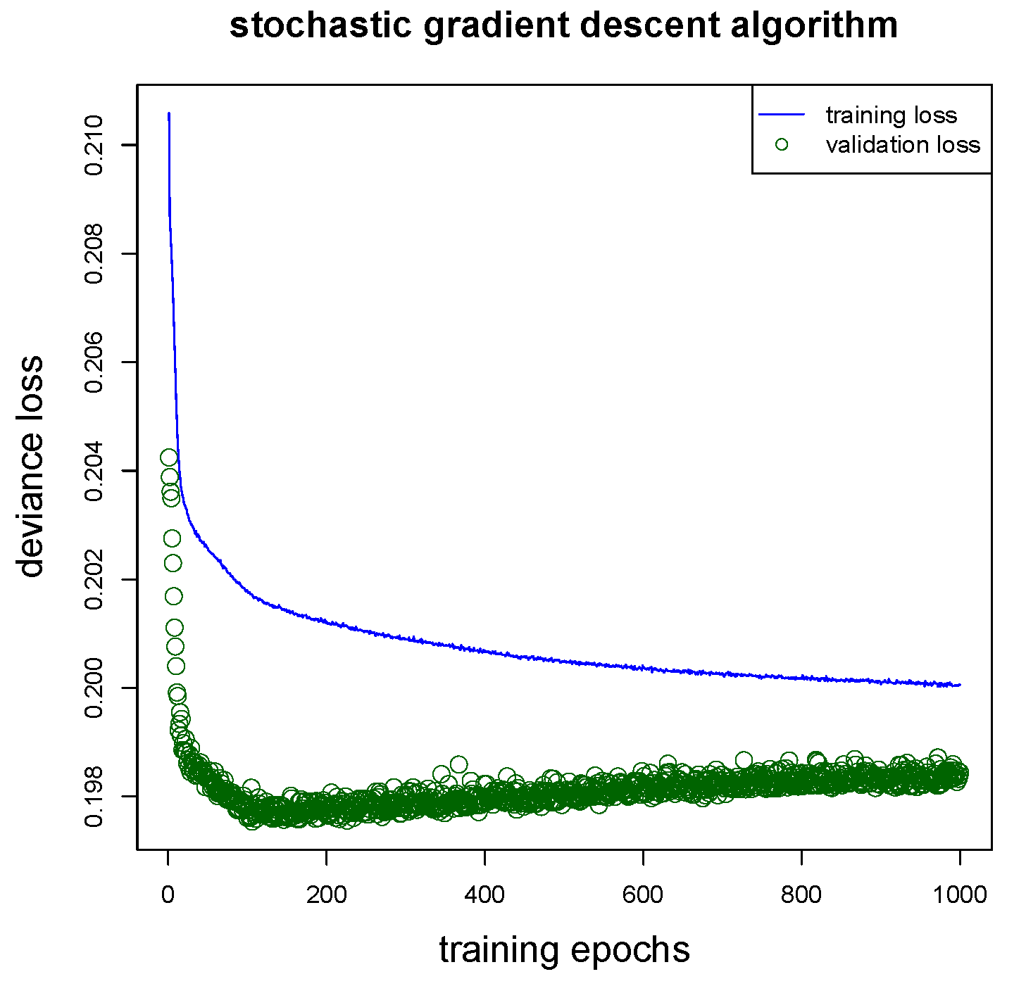
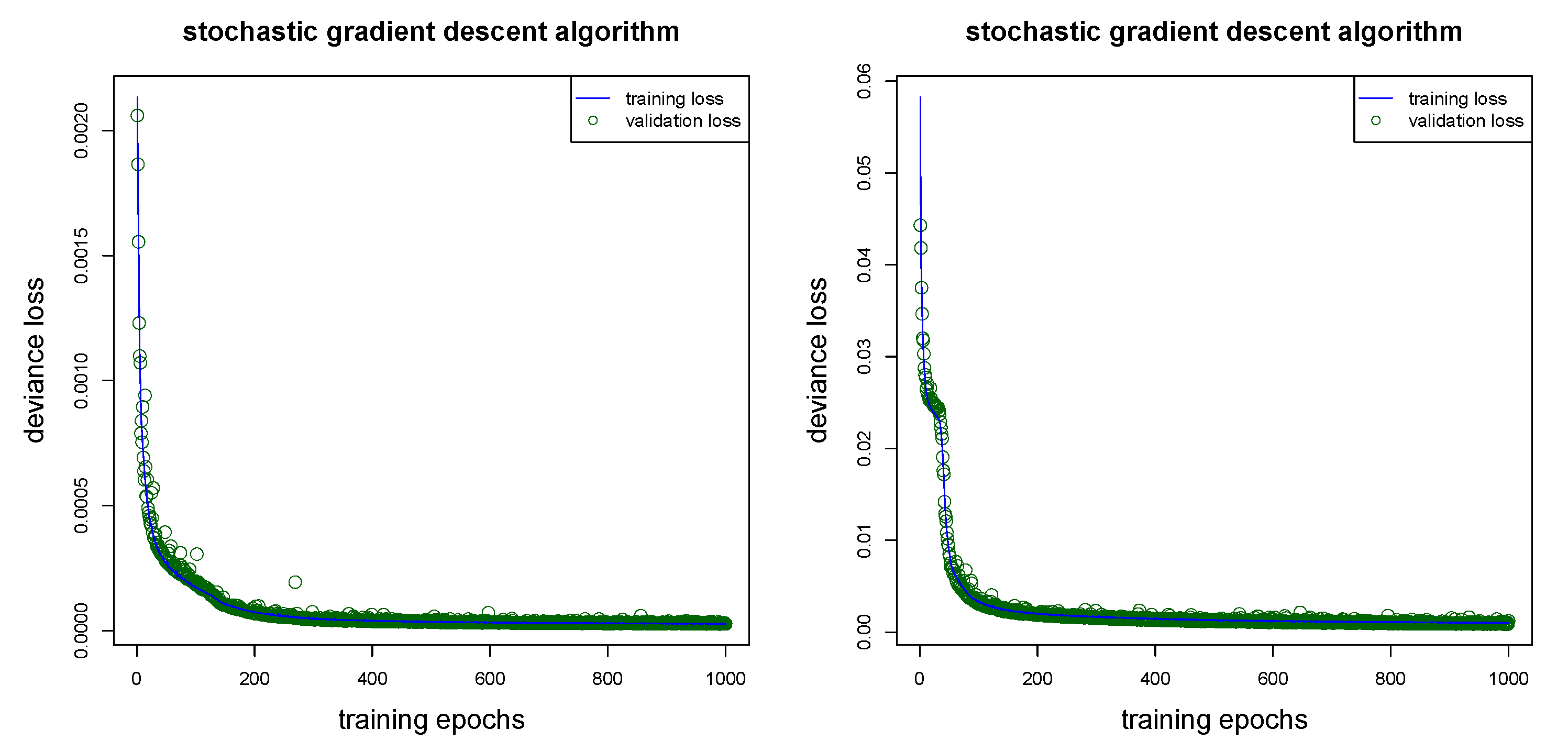
We are now ready to fit this network regression model to the learning data set $\mathcal{D}$. Running this algorithm involves some more choices. First of all, we need to ensure that the network does not over-fit to the learning data $\mathcal{D}$. To ensure this we partition at random 9:1 the learning data into a training data set ${\mathcal{D}}^{(-)}$ and a validation data set $\mathcal{V}$. The network parameter is learned on the training data ${\mathcal{D}}^{(-)}$ and over-fitting is tracked on the validation data $\mathcal{V}$. We run the nadam gradient descent algorithm over 1000 epochs on random mini-batches of size 5000 from the training data ${\mathcal{D}}^{(-)}$. Using a callback we retrieve the network parameter that has the smallest (validation) loss on $\mathcal{V}$, this is exactly the stopping rule that we set in place, here. This is illustrated in Figure 1 giving training losses on ${\mathcal{D}}^{(-)}$ in blue color and validation losses on $\mathcal{V}$ in green color. We observe that the validation loss increases after roughly 150 training epochs (green color), and we retrieve the network parameter with the lowest validation loss.

The fact that the resulting network model has been received by an early stopping of the gradient descent algorithm implies that this network has a bias w.r.t. the learning data $\mathcal{D}$. For this reason we additionally apply the bias regularization step proposed in Section 3.4 of Wüthrich (2019), see Listing 5 in Wüthrich (2019). This gives us an estimated network parameter ${\widehat{\mathit{\beta }}}^{\left(1\right)}$ and corresponding mean estimates ${\widehat{\mu }}_i^{\left(1\right)}$ for all insurance policies in $\mathcal{D}$ and $\mathcal{T}$. This procedure leads to the results on line (d) of

Table 2. (a) Homogeneous model not using any feature information, (b,c) generalized linear model (GLM) and boosting regression models both from Table 11 in Noll et al. (2018), (d) network regression model as outlined above for given seed $j=1$, (e) averaged losses over 400 network calibrations (with standard errors in brackets), (f) nagging predictor; losses are in ${10}^{-2}$.

	In-Sample		Out-of-Sample
	Loss on $\mathcal{D}$		Loss on $\mathcal{T}$
(a) homogeneous model	32.935		33.861
(b) generalized linear model	31.267		32.171
(c) boosting regression model	30.132		31.468
(d) network regression model (seed $j=1$)	30.184		31.464
(e) average over 400 network calibrations	30.230	(0.089)	31.480	(0.061)
(f) nagging predictor for $M=400$	30.060		31.272

.

We compare the network results to the ones received in Table 11 of Noll et al. (2018), and we conclude that our network approach is competitive with these other methods (being a classical GLM and a boosting regression model), see the out-of-sample losses on lines (a)–(d).

Remark 3.

Our analysis is based on claim counts observations, therefore, the Poisson model is the canonical choice. As mentioned in Remark 1, depending on the underlying modeling problem other distributional choices from the EDF may be more appropriate. In any of these other model choices the proposed methodology works similarly, only minor changes to theRcode in Listing A1 will be necessary:

• Firstly, the complexity of the network architecture should be adapted to the problem, both the sizes of the hidden layers and the depth of the network will vary with the complexity of the problem and the complexity of the regression function. In general, the bigger the network the better the approximation capacity (this follows from the universality theorems). This says that the chosen network should have a certain complexity otherwise it will be not sufficiently flexible to approximate the true (but unknown) regression function. On the other hand, for computational reasons, the chosen network should not be too large.
• Secondly, different distributions will require different choices of loss functions on line 25 of Listing A1. Some loss functions are already implemented in thekeraslibrary, others will require custom loss functions. An example of a custom loss function implementation is given in Listing 2 of Delong et al. (2020). In general, the loss function of any density that allows for an EDF representation can be implemented inkeras.
• Thirdly, we could add more specialized layers to the network architecture of Listing A1. For instance, we could add dropout layers after each hidden layer on lines 15–17 of Listing A1, for dropout layers see Srivastava et al. (2014). Dropout layers add an additional element of randomness during training, because certain network connections are switched off (at random) for certain training steps when using dropout. This switching off of connections acts as regularization during training because it prevents certain neurons from over-fitting to special tasks. In fact, under certain assumptions one can prove that dropout acts similarly to ridge regularization, see Section 18.6 in Efron and Hastie (2016). In our study we refrain from using dropout.

5.5. Comparison of Different Network Calibrations

The issue with the network result on line (d) of Table 2 now is that it involves quite some randomness:

(R1)

we randomly split learning data $\mathcal{D}$ into training data ${\mathcal{D}}^{(-)}$ and validation data $\mathcal{V}$;

(R2)

we randomly split training data ${\mathcal{D}}^{(-)}$ into mini-batches of size 5000 (to more efficiently calculate gradient descent steps); and

(R3)

we randomly choose the starting point of the gradient descent algorithm; the default initialization in keras is the glorot_uniform initialization which involves simulation from uniform distributions.

Changing seeds in these points (R1)–(R3) will change the network regression parameter estimate ${\widehat{\mathit{\beta }}}^{\left(j\right)}$ and, hence, the results. For this study we explore the randomness of changing the seeds in (R1)–(R3). However, one may also be interested in sensitivities of results when changing sizes of the mini-batches, hyper-parameters of the gradient descent methods, or when using stratified versions of validation data. We will not explore this here.

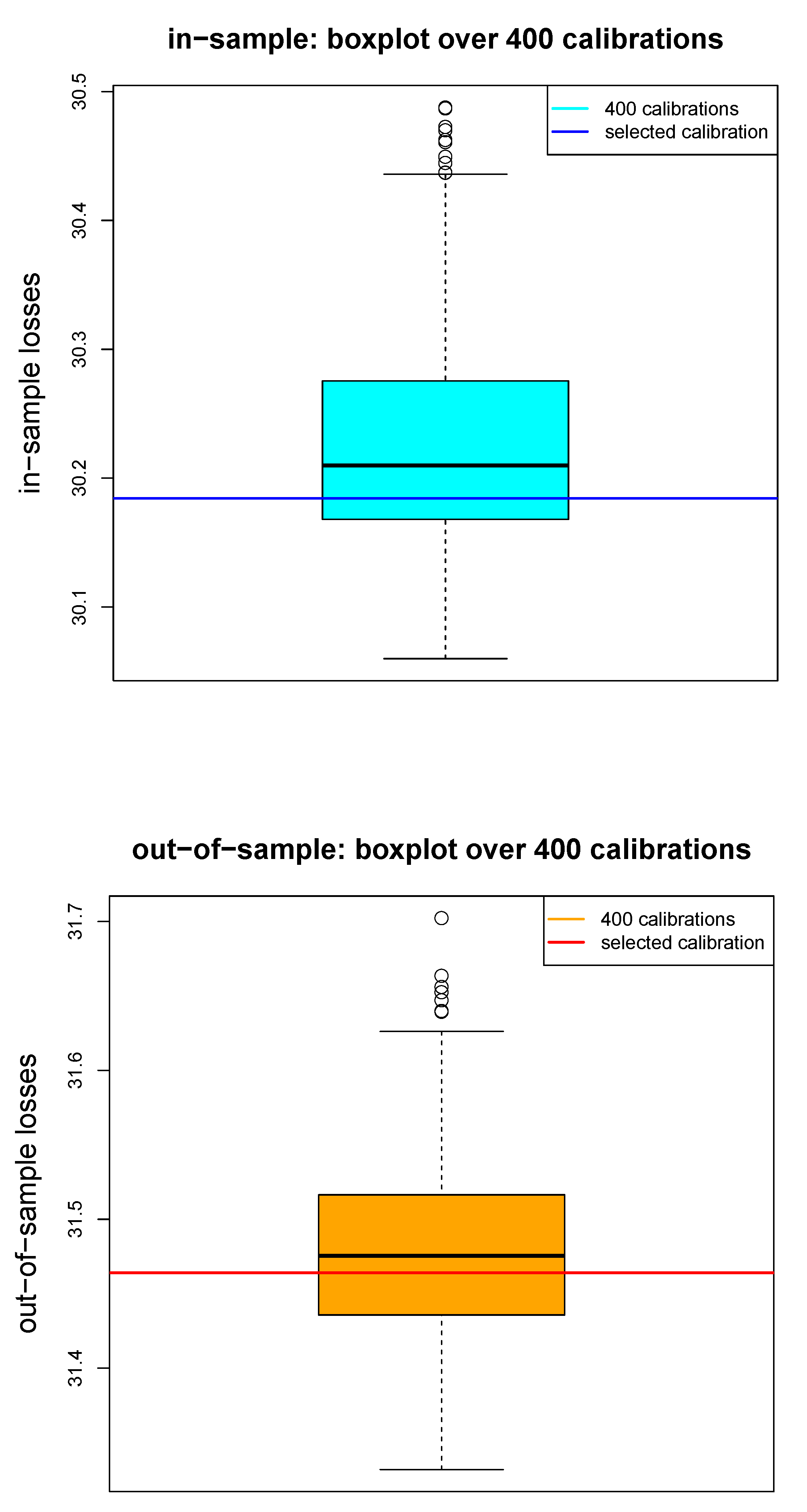
We run the above calibration procedure under identical choices of all hyper-parameters, but we choose different seeds for the random choices (R1)–(R3). The boxplot in Figure 2 shows the in-samples losses $\mathcal{L}(\mathcal{D};{\widehat{\mathit{\beta }}}^{(j)})$ and out-of-samples losses $\mathcal{L}(\mathcal{T};{\widehat{\mathit{\beta }}}^{(j)})$ over 400 network calibrations ${\widehat{\mathit{\beta }}}^{(j)}$ by only randomly changing the seeds in the above mentioned points (R1)–(R3). We note that these losses have a rather large range which indicates that results of single network calibrations are not very robust. We can calculate empirical mean and standard deviation for the 400 seeds j given by

$$\overline{\mathcal{L}}(\mathcal{T};{\widehat{\mathit{\beta }}}^{(1:400)})=\frac{1}{400}{\displaystyle \sum _{j=1}^{400}}\mathcal{L}(\mathcal{T};{\widehat{\mathit{\beta }}}^{(j)})\mathrm{and}\sqrt{\frac{1}{399}{\displaystyle \sum _{j=1}^{400}}{\left(\overline{\mathcal{L}}(\mathcal{T};{\widehat{\mathit{\beta }}}^{(1:400)})-\mathcal{L}(\mathcal{T};{\widehat{\mathit{\beta }}}^{(j)})\right)}^2}.$$

The first gives an estimate for the expected generalization loss Equation (8) averaged over the corresponding portfolios. We emphasize in notation ${\widehat{\mathit{\beta }}}^{(1:400)}$ that we do not average over network parameters, but over deviance losses on individual network parameters ${\widehat{\mathit{\beta }}}^{\left(j\right)}$. The resulting numbers are given on line (e) of Table 2. This shows that the early stopped network calibrations have quite significant differences, which motivates the study of the nagging predictor.

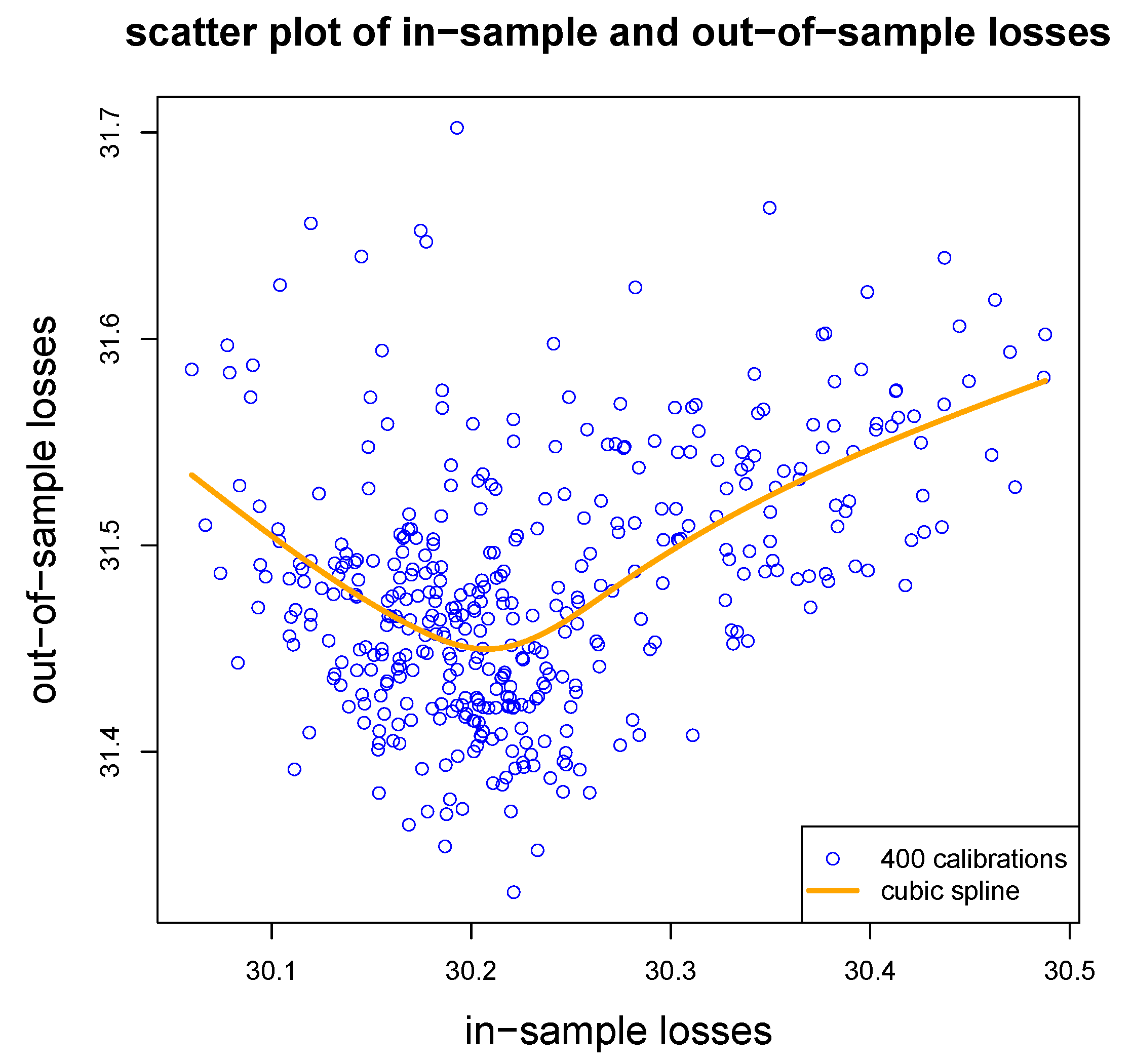
Figure 3 gives a scatter plot of in-sample and out-of-sample losses over the 400 different runs of the gradient descent fitting (complemented with a natural cubic spline). We note in this example that both small and big in-sample losses do not lead to favorable generalization, small in-sample losses may indicate over-fitting and big out-of-sample losses may indicate the that early stopping rule has not found a good model based on the validation data $\mathcal{V}$.

5.6. Nagging Predictor

We are now in the situation where we are able to calculate the nagging predictors ${\overline{\mu }}_t^{\left(M\right)}$ over the test data set $\mathcal{T}$. For $M\to \infty$ this provides us with empirical counterparts of Propositions 3 and 4. We therefore consider for $M\ge 1$ the sequence of out-of-sample losses, see Equation (12),

$$\mathcal{L}(\mathcal{T};{\overline{\overline{\mu }}}_{t=1,\dots ,m}^{\left(M\right)})=\frac{1}{m}\sum _{t=1}^m\delta (Y_t^{†},{\overline{\overline{\mu }}}_t^{\left(M\right)}),$$

where ${\overline{\mu }}_t^{\left(M\right)}$ are the nagging predictors Equation (13) received from the i.i.d. sequence ${\widehat{\mu }}_t^{\left(j\right)}=\mu ({\mathit{x}}_t^{†},{\widehat{\mathit{\beta }}}^{(j)})$ and, again, where the i.i.d. property is conditional on $\mathcal{D}$ and refers to the i.i.d. starting points chosen to start the gradient descent fitting algorithm.

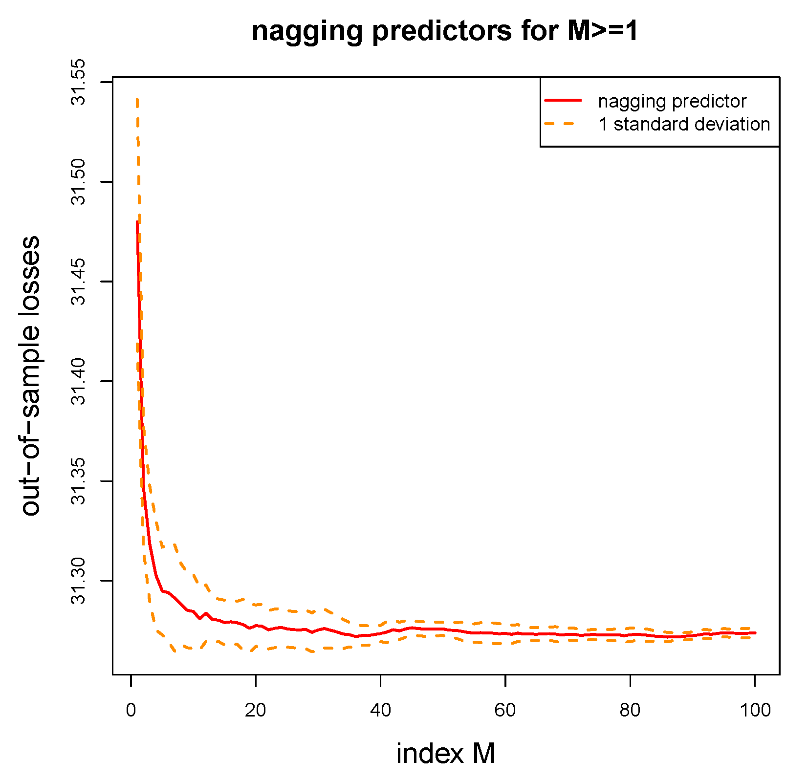
Figure 4 gives the out-of-sample losses of the nagging predictors $\mathcal{L}(\mathcal{T};{\overline{\overline{\mu }}}_{t=1,\dots ,m}^{\left(M\right)})$ for $M=1,\dots ,100$. Most noticeable is that nagging leads to a substantial improvement in out-of-sample losses, for $M\to \infty$ the out-of-sample loss converges to 31.272 which is much smaller then the figures reported on lines (b)–(e) of Table 2, in fact, the out-of-sample loss decreases by more than 3 standard deviations (as reported on line (e) of Table 2). From this we conclude that nagging helps to improve the predictive model substantially. From Figure 4 we also observe that this convergence mainly takes place over the first 20 aggregating steps in our example. That is, we need to aggregate over roughly 20 network calibrations ${\widehat{\mathit{\beta }}}^{\left(j\right)}$ to get the maximal predictive power. The dotted orange lines in Figure 4 give corresponding 1 standard deviation confidence bounds (received by repeating the nagging procedure for different seeds). To get sufficiently small confidence bounds in our example we need to average over roughly 40 network calibrations.

Conclusion 1.

Nagging helps to sufficiently improve out-of-sample performance of network regression models. In our example we need to average over 20 different calibrations to get optimal predictive power, and we need an average of 40 calibrations to ensure that we cannot further improve this predictive power.

5.7. Pricing of Individual Insurance Policies

In the previous sections we have proved that nagging successfully improves models. However, all these considerations have mainly been based on portfolio considerations, i.e., our focus has been on the question whether the insurance company has a model that gives good predictive power to predict the portfolio claim amount. For insurance pricing, this is not sufficient because we should also ensure that we have robustness of prices on an individual insurance policy level. In this section we analyze by how much individual insurance policy prices may differ if we select two different network calibrations ${\widehat{\mathit{\beta }}}^{\left(j\right)}$ and ${\widehat{\mathit{\beta }}}^{\left(j^{\prime }\right)}$. This will tell us whether aggregating over 20 or 40 network calibrations is sufficient as stated in Conclusion 1. Naturally, we expect that we need to average over more networks because the former statement includes an average over $\mathcal{T}$, i.e., over $m=\mathrm{67,801}$ insurance policies (though there is dependence between these policies because they simultaneously use the same network parameter estimate ${\widehat{\mathit{\beta }}}^{\left(j\right)}$).

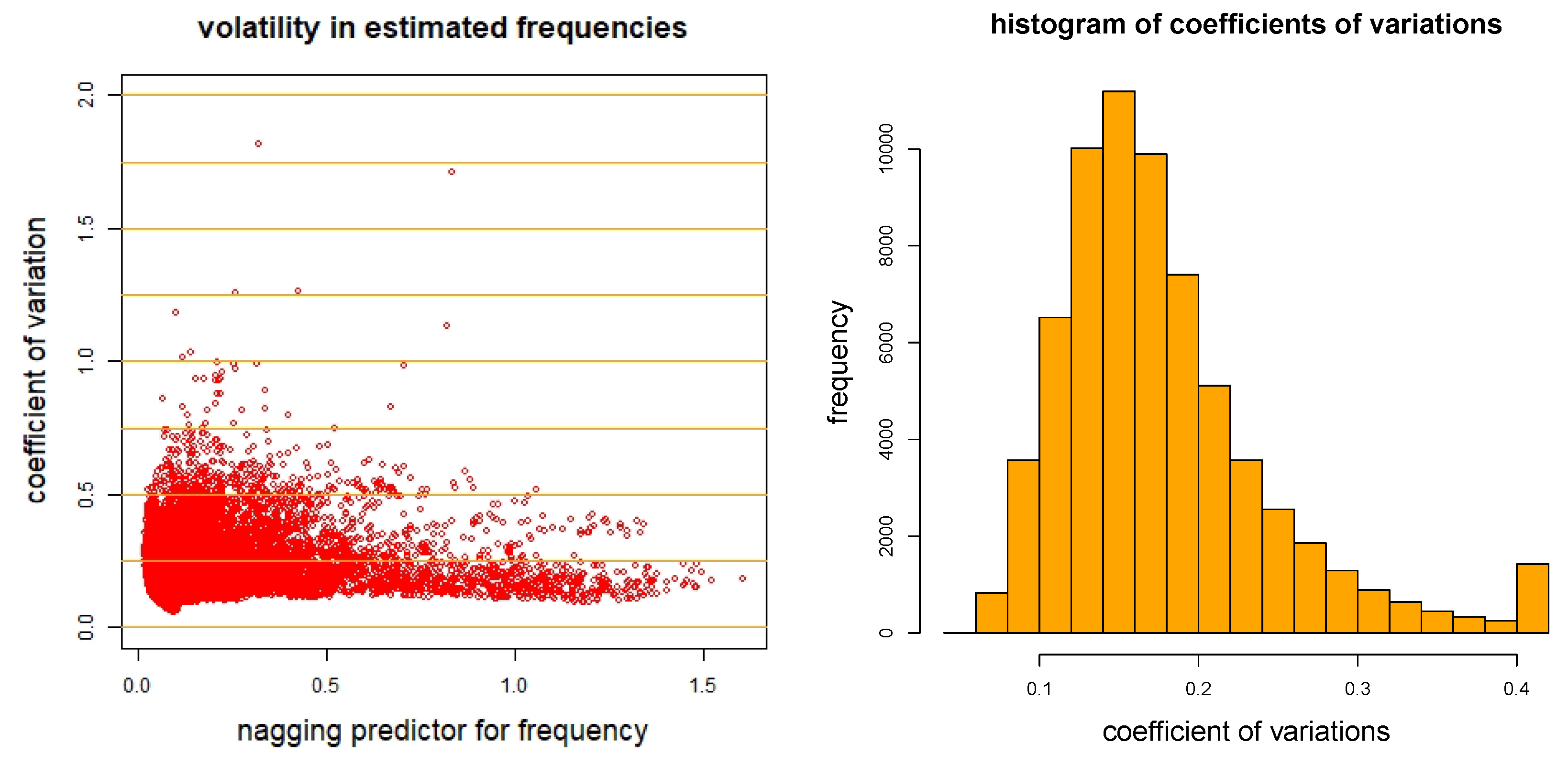
To analyze this question on individual insurance policies we calculate for each policy $t=1,\dots ,m$ of the test data $\mathcal{T}$ the nagging predictor ${\overline{\mu }}_t^{\left(M\right)}$ over $M=400$ different network calibrations ${\widehat{\mathit{\beta }}}^{\left(j\right)}$, $j=1,\dots ,M$, and we calculate the empirical coefficients of variation in the individual network predictors given by

$${\widehat{\mathrm{CoV}}}_t=\frac{{\widehat{\sigma }}_t}{{\overline{\overline{\mu }}}_t^{\left(M\right)}}=\frac{\sqrt{\frac{1}{M-1}{\sum }_{j=1}^M{\left({\widehat{\mu }}_t^{\left(j\right)}-{\overline{\overline{\mu }}}_t^{\left(M\right)}\right)}^2}}{{\overline{\overline{\mu }}}_t^{\left(M\right)}},$$

(15)

these are the empirical standard deviations normalized by the corresponding mean estimates. We plot these coefficients of variations ${\widehat{\mathrm{CoV}}}_t$ in Figure 5 (lhs) against the nagging predictors ${\overline{\mu }}_t^{\left(M\right)}$ for each single insurance policy $t=1,\dots ,m$ (out-of-sample on $\mathcal{T}$). Figure 5 (rhs) shows the resulting histogram. We observe that on most insurance policies (73%) we have a coefficient of variation of less than 0.2, however, on 11 of the $m=\mathrm{67,801}$ insurance policies we have a coefficient of variation bigger then 1. Thus, for the latter, if we average over 400 different network calibrations ${\widehat{\mathit{\beta }}}^{\left(j\right)}$ we still have an uncertainty of $1/\sqrt{400}=0.05$, i.e., the prices have a precision of 5% to 10% in these latter cases (this is always conditional given $\mathcal{D}$). From this we conclude that on individual insurance policies we need to aggregate over a considerable number of networks to receive stable network regression prices.

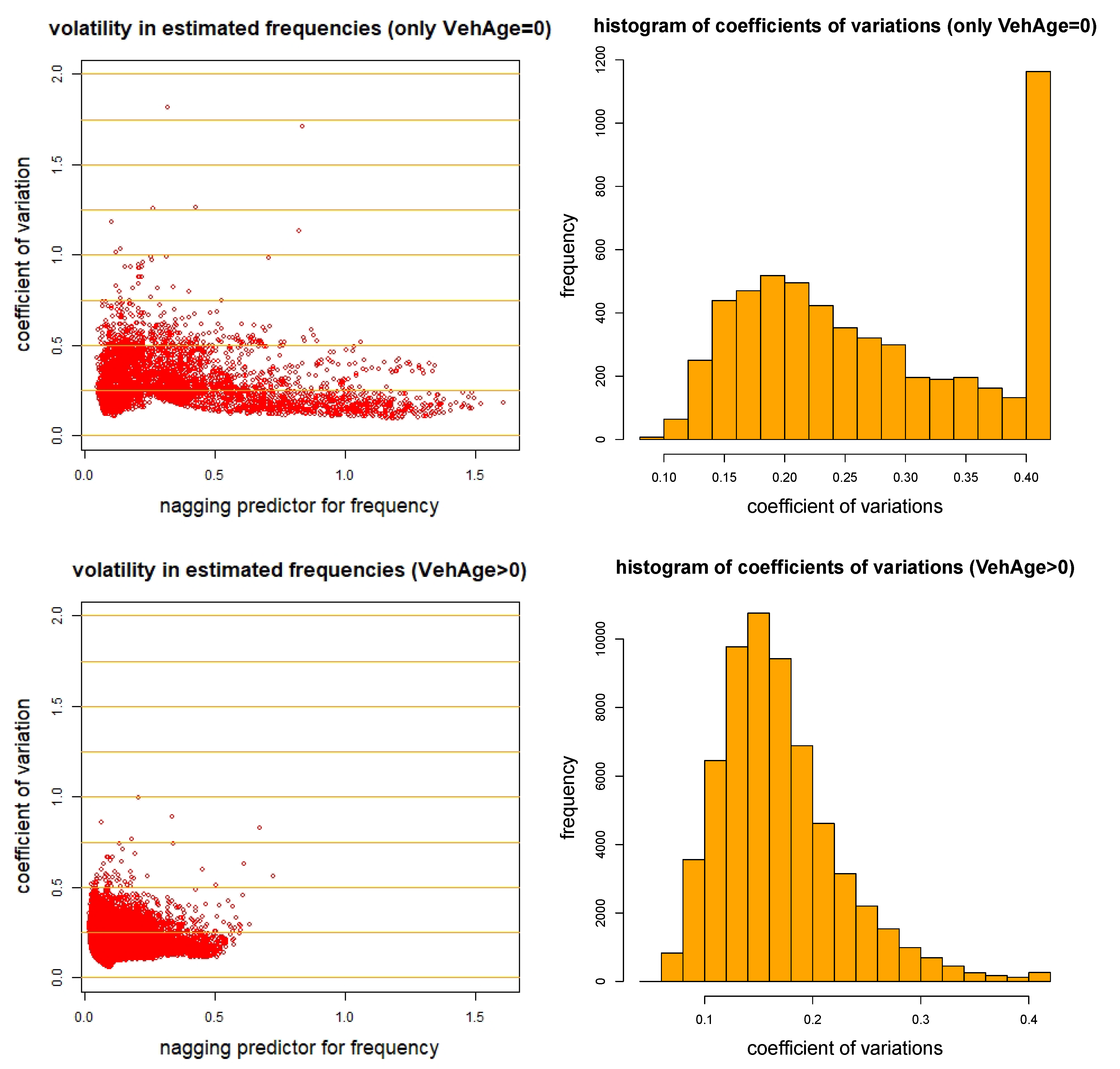
We show these 11 insurance policies with a coefficient of variation bigger 1 in Listing 2. Striking is that all these insurance policies have vehicle age $\mathtt{VehAge}=0$. In Figure 6 (top row) we show a scatter plot and histogram of these insurance policies, and Figure 6 (bottom row) gives the corresponding graphs for $\mathtt{VehAge}>0$. We indeed confirm that mainly the policies with $\mathtt{VehAge}=0$ are difficult to price. From the histogram in Figure 5 (rhs) we receive in total 1423 policies that have a coefficient of variation ${\widehat{\mathrm{CoV}}}_t$ bigger than 0.4, and in view of Figure 6 (rhs), 1163 of these insurance policies have $\mathtt{VehAge}=0$.

Listing 2. Policies with high coefficients of variation ${\widehat{\mathrm{CoV}}}_t$.

Listing 2. Policies with high coefficients of variation ${\widehat{\mathrm{CoV}}}_t$.

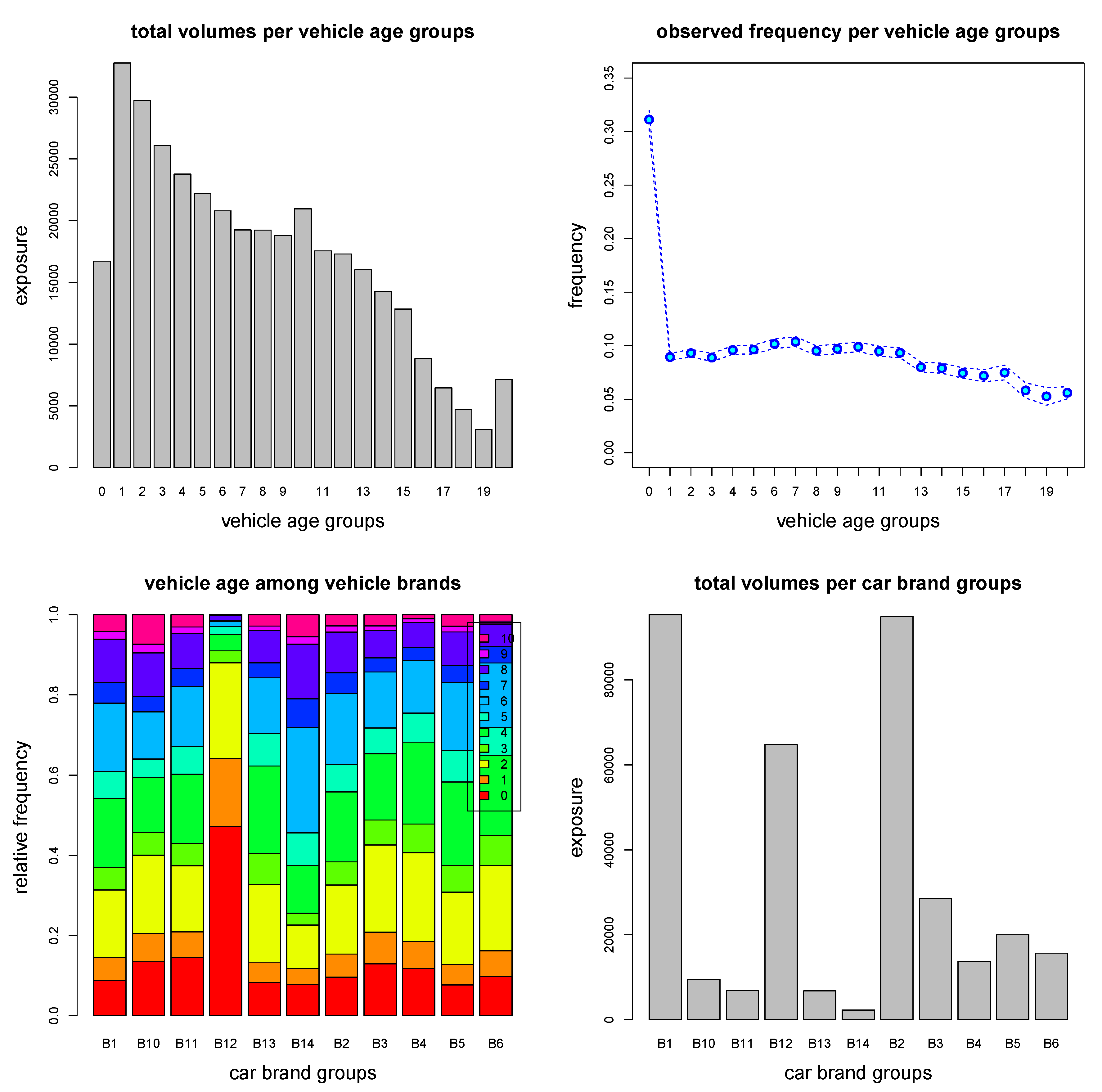
To better understand this uncertainty in $\mathtt{VehAge}=0$, we provide some empirical plots for those vehicles with age 0; these plots are taken from Noll et al. (2018). Figure 7 shows the total exposure per vehicle age (top-lhs), the empirical frequency per vehicle age (top-rhs), the vehicle ages per vehicle brands (bottom-lhs) and total exposures per vehicle brand (bottom-rhs). From these graphs we observe that vehicle age 0 has a completely different frequency than all other vehicle ages (Figure 7, top-rhs). Moreover, vehicle age 0 is dominated by vehicle brand B12 (Figure 7, bottom). It seems in view of Listing 2 that this configuration results in quite some uncertainty in frequency prediction, note that 1011 of the 1163 insurance policies with vehicle age 0 and a coefficient of variation bigger than 0.4 are cars of vehicle brand B12. Naturally, in a next step we would have to analyze vehicle age 0 and vehicle brand B12 in more depth, we suspect that these could likely be rental cars (or some other special cases). Unfortunately, there is no further information available for this data set that allows us to investigate this problem more thoroughly. We remark that König and Loser (2020) come to a similar conclusion for cars of vehicle brand B12 with vehicle age 0, see regression tree in Chapter 1.2 of König and Loser (2020) where furthermore the split w.r.t. vehicle gas is important.

5.8. Meta Network Regression Model

From the previous sections we conclude that the nagging predictor substantially improves the predictive model. Nevertheless, the nagging predictor may not be fully satisfactory in practice. The difficulty is that it involves aggregating over $M=400$ predictors ${\widehat{\mu }}_i^{\left(j\right)}$ for each policy i. Such blended predictors (and models) are not easy to maintain nor is it simple to study model properties, updating models with new observations, etc., for instance, if we have a new insurance policy having covariate $\mathit{x}$, then we need to run this new insurance policy through all $M=400$ networks to receive the price. For this reason we propose to build a meta model that fits a new network to the nagging predictors ${\overline{\mu }}_i^{\left(M\right)}$, $i=1,\dots ,n$. In the wider machine learning literature, building such meta models is also referred to as “model distillation”, see Hinton et al. (2015). Since these nagging predictors are aggregated predictors over M network models, and since the network regression functions themselves are smooth functions in input variables (at least in the continuous features), the nagging predictors describe smooth surfaces. Therefore, it is comparably simple to fit a network to the smooth surface described by nagging predictors ${\overline{\mu }}_i^{\left(M\right)}$, $i=1,\dots ,n$, and over-fitting will not be an issue. To build this meta model we use exactly the same network architecture as above, and as outlined in Listing A1 in the Appendix A. The only parts that we change are the loss function and the response variables. We replace the original claim count responses $Y_i$ by the nagging predictors ${\overline{\mu }}_i^{\left(M\right)}$, and for the loss function we choose the square loss function. We can either choose an unweighted square loss function or we can weight the individual observations with the inverse standard deviation estimates $1/{\widehat{\sigma }}_i$, see Equation (15), the latter reflects the idea of giving more weight to predictors that have less uncertainty. In fact, the latter is a little bit similar to Zhou et al. (2002) where the authors argue that equally weighting over network predictors is non-optimal. Our approach is slightly different here because we do not weight networks, but we weight nagging predictors of individual insurance policies to receive better rates of convergence for meta model training.

We present the gradient descent fitting performance in Figure 8 and the resulting in-sample and out-of-sample losses in

Table 3. (d)–(f) Network regression models from Table 2 compared to meta models (g1)–(g2); losses are in ${10}^{-2}$.

	In-Sample		Out-of-Sample
	Loss on $\mathcal{D}$		Loss on $\mathcal{T}$
(d) network regression model (seed $j=1$)	30.184		31.464
(e) average over 400 network calibrations	30.230	(0.089)	31.480	(0.061)
(f) nagging predictor for $M=400$	30.060		31.272
(g1) meta network model (un-weighted)	30.260		31.342
(g2) meta network model (weighted)	30.257		31.332

. We conclude that the weighted version of the square loss has better convergence properties in gradient descent fitting, and the resulting model has a better loss performance, compare lines (g1) and (g2) of Table 3. The resulting meta model on line (g2) is slightly worse than the nagging predictor model on line (f), however, substantially better than the individual network models (d)–(e) and much more easy in handling than the nagging predictor. For this reason, we are quite satisfied by the meta model, and we propose to hold on to this model for further analysis and insurance pricing.

Remark 4.

We have mentioned in Remark 3 that model implementation will slightly change if we move from our Poisson example to another distributional example, for instance, the loss function has to be adapted to the choice of the distribution function. The last step of fitting a meta model, however, does not require any changes. Note that the meta model fits a regression function to another regression function (which is the nagging predictor in our case). This fitting uses the square loss as the objective function, and the nature of the distribution function of the observations is not important because we fit a deterministic function to another deterministic function here.

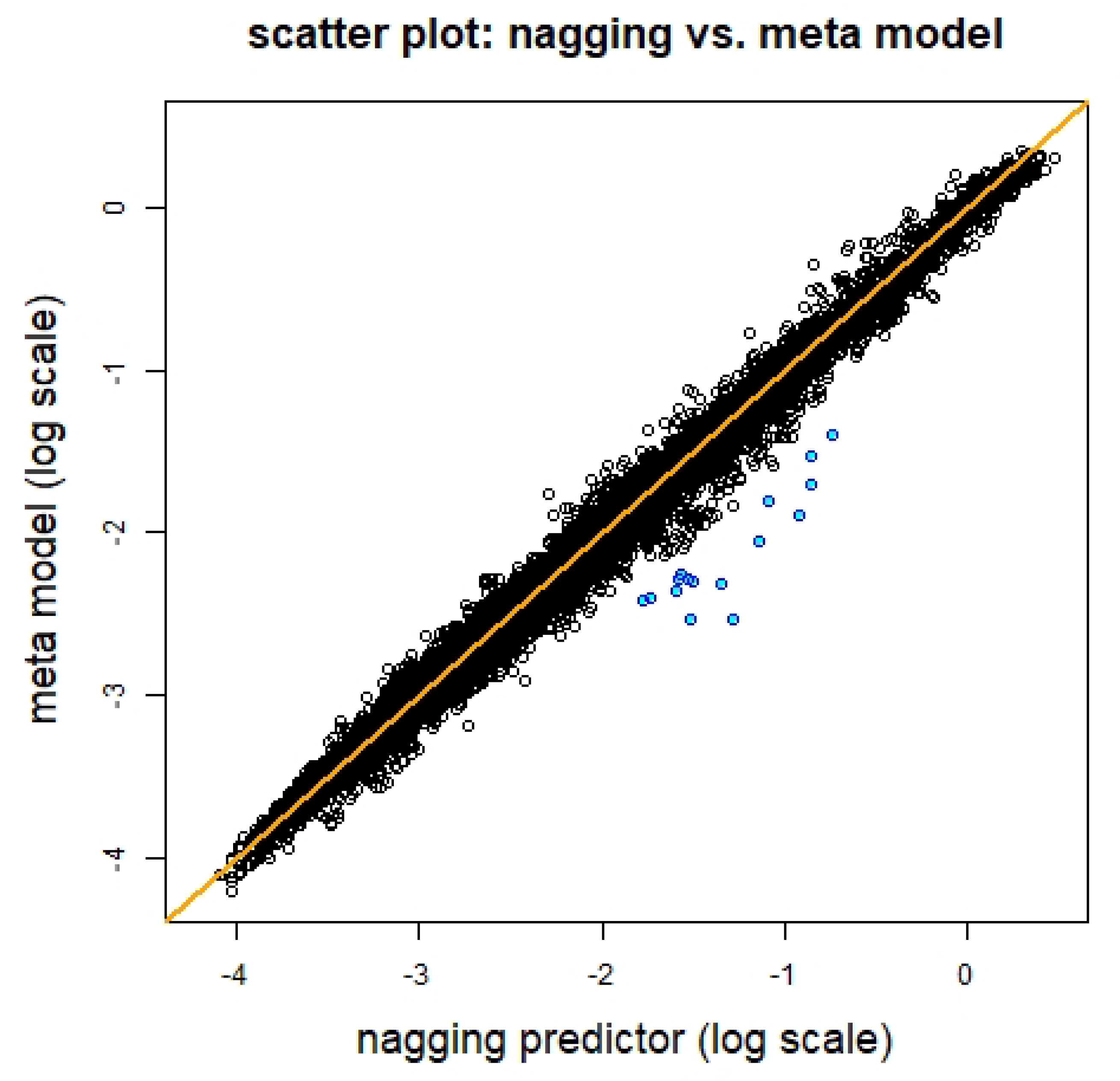
In Figure 9 we present the two predictors in a scatter plot, we observe that they are reasonably equal, the biggest differences are highlighted in blue color, and they refer to policies with vehicle age 0, that is, the feature component within the data that is the most difficult to fit with the network model.

We provide a concluding analysis of this meta model. As emphasized in Section 7 of Richman et al. (2019), we analyze and try to understand the representations learned in the last hidden layer of the network over all insurance policies. In view of Equation (1) this means that we study the learned representations for $t=1,\dots ,m$ given by

$${\mathit{x}}_t^{†}\mapsto {\breve{\mathit{x}}}_t^{†}=\left({\mathit{z}}^{\left(d\right)}\circ \cdots \circ {\mathit{z}}^{\left(1\right)}\right)\left({\mathit{x}}_t^{†}\right)\in {\mathbb{R}}^{q_d+1},$$

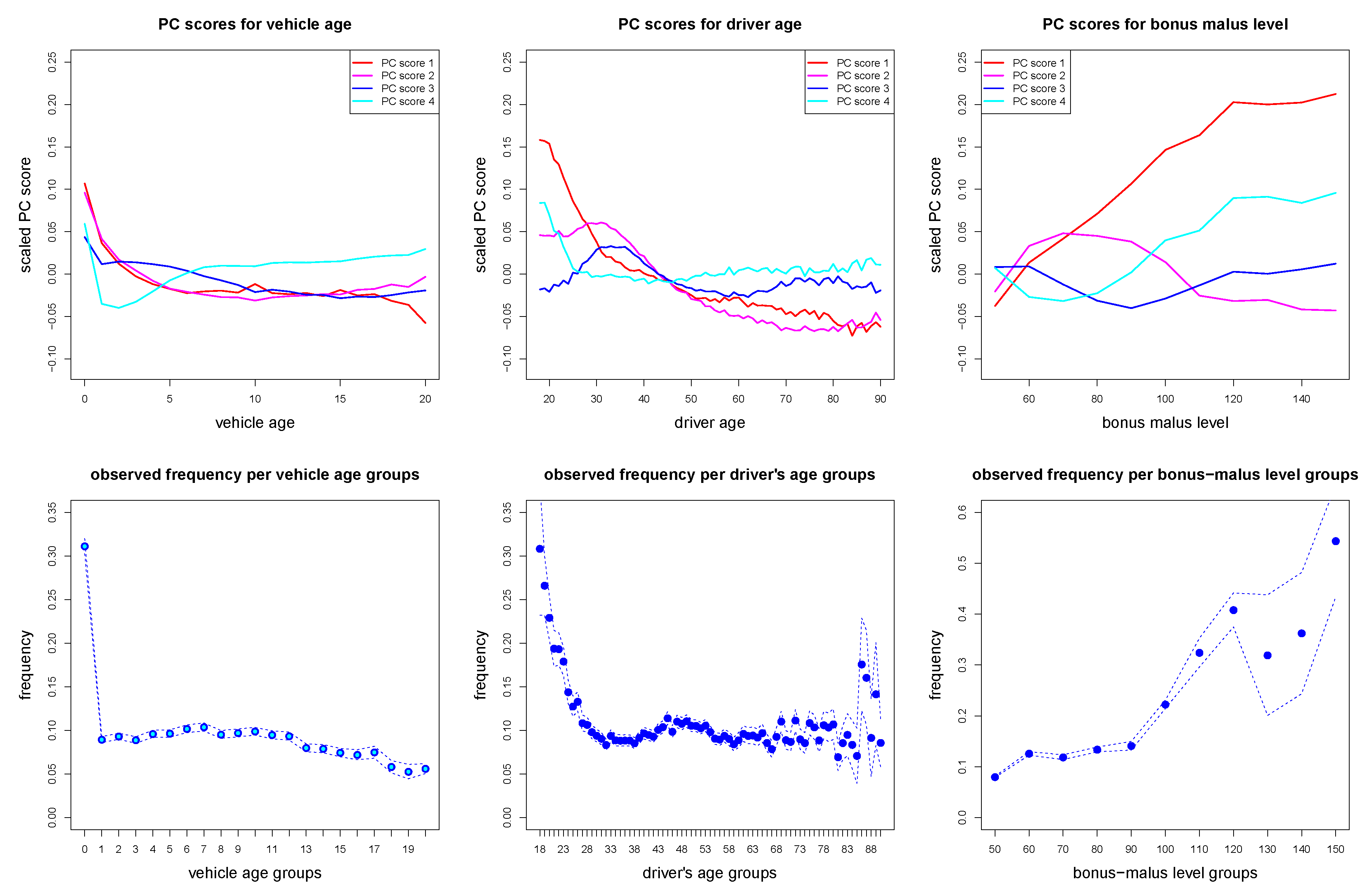
to which the GLM step with readout parameter ${\mathit{\beta }}^{(d+1)}\in {\mathbb{R}}^{q_d+1}$ is applied to. In our example of Listing A1 we have $d=3$ hidden layers with $q_3=10$ hidden neurons in this last hidden layer. In order to illustrate the learned representations we apply a principal component analysis (PCA) to these learned representations ${\left({\breve{\mathit{x}}}_t\right)}_{t=1,\dots ,m}$. This provides us with the principal component (PC) scores for each policy t and the corresponding singular values ${\lambda }_{q_3}\ge \dots \ge {\lambda }_1\ge 0$. Note that these PC scores are ordered w.r.t. importance measured by the singular values. We scale the individual PC scores $k=1,\dots ,q_3$ with $\sqrt{{\lambda }_k}$ to reflect this importance. In Figure 10 (top row) we plot these scaled PC scores for the first 4 principal components and averaged per vehicle age (lhs), driver age (middle), and bonus malus level (rhs). We remark that these 3 feature components are the most predictive ones according to the descriptive analysis in Noll et al. (2018). From Figure 10 (top row) we observe that the first principal component (in red color) reflects the marginal empirical frequencies illustrated in Figure 10 (bottom row), thus, the first PC reflects the influence of each of these three explanatory variables on the regression function, and higher order PCs are used to refine this picture and model interactions between feature components.

6. Conclusions and Outlook

This work has defined the nagging predictor which produces accurate and stable portfolio predictions on the basis of random network calibrations, and it provided convergence results in the context of Tweedie’s compound Poisson generalized linear models. Focusing on an example in motor third-party liability insurance pricing, we have shown that stable portfolio results are achieved after 20 network training runs, and by increasing the number of network training runs to 400, we have shown that quite stable results are produced at the level of individual policies, which is an important requirement for the use of networks for insurance pricing, and more general actuarial tasks. The coefficient of variation of the nagging predictor is shown to be a useful data-driven metric for measuring the relative difficulty with which a network is able to fit to individual training examples, and we have used it to calibrate an accurate meta network which approximates the nagging predictor. Whereas this work has examined the stability of network predictions in the case of a portfolio at a point in time, another important aspect of consistency within insurance is stable pricing over time, thus, future work could consider methods for stabilizing network predictions as new information becomes available.

References

- Breiman, Leo. 1996. Bagging predictors. Machine Learning 24: 123–40. [Google Scholar] [CrossRef] [Green Version]
- Bühlmann, Peter, and Bin Yu. 2002. Analyzing bagging. The Annals of Statistics 30: 927–61. [Google Scholar] [CrossRef]
- Cybenko, George. 1989. Approximation by superpositions of a sigmoidal function. Mathematics of Control, Signals, and Systems 2: 303–14. [Google Scholar] [CrossRef]
- Delong, Łukasz, Matthias Lindholm, and Mario V. Wüthrich. 2020. Making Tweedie’s compound Poisson model more accessible. SSRN, 3622871, Version of 8 June. Available online: https://papers.ssrn.com/sol3/papers.cfm?abstract_id=3622871 (accessed on 1 July 2020). [CrossRef]
- Di Persio, Luca, and Oleksandr Honchar. 2016. Artificial neural networks architectures for stock price prediction: Comparisons and applications. International Journal of Circuits, Systems and Signal Processing 10: 403–13. [Google Scholar]
- Dietterich, Thomas G. 2000a. An experimental comparison of three methods for constructing ensembles of decision trees: Bagging, boosting, and randomization. Machine Learning 40: 139–57. [Google Scholar] [CrossRef]
- Dietterich, Thomas G. 2000b. Ensemble methods in machine learning. In Multiple Classifier Systems. Edited by Josef Kittel and Fabio Roli. Lecture Notes in Computer Science, 1857. Berlin and Heidelberg: Springer, pp. 1–15. [Google Scholar]
- Dutang, Christophe, and Arthur Charpentier. 2019. CASdatasets R Package Vignette. Reference Manual, November 13, 2019. Version 1.0-10. Available online: http://dutangc.free.fr/pub/RRepos/web/CASdatasets-index.html (accessed on 13 November 2019).
- Efron, Bradley, and Trevor Hastie. 2016. Computer Age Statistical Inference. Cambridge: Cambridge University Press. [Google Scholar]
- Goodfellow, Ian, Yoshua Bengio, and Aaron Courville. 2016. Deep Learning. Cambridge: MIT Press. [Google Scholar]
- Hinton, Geoffrey, Oriol Vinyals, and Jeff Dean. 2015. Distilling the knowledge in a neural network. Version 9 March. arXiv arXiv:1503.02531. [Google Scholar]
- Hornik, Kurt, Maxwell B. Stinchcombe, and Halbert White. 1989. Multilayer feedforward networks are universal approximators. Neural Networks 2: 359–66. [Google Scholar] [CrossRef]
- du Jardin, Philippe. 2016. A two-stage classification technique for bankruptcy prediction. European Journal of Operations Research 254: 236–52. [Google Scholar] [CrossRef]
- Jørgensen, Bent. 1986. Some properties of exponential dispersion models. Scandinavian Journal of Statistics 13: 187–97. [Google Scholar]
- Jørgensen, Bent. 1987. Exponential dispersion models. Journal of the Royal Statistical Society. Series B (Methodological) 49: 127–45. [Google Scholar]
- Jørgensen, Bent, and Marta C. Paes de Souza. 1994. Fitting Tweedie’s compound Poisson model to insurance claims data. Scandinavian Actuarial Journal 1994: 69–93. [Google Scholar] [CrossRef]
- König, Daniel, and Friedrich Loser. 2020. GLM, neural network and gradient boosting for insurance pricing. Kaggle. Available online: https://www.kaggle.com/floser/glm-neural-nets-and-xgboost-for-insurance-pricing (accessed on 10 July 2020).
- LeCun, Yann, Yosua Bengio, and Geoffrey Hinton. 2015. Deep learning. Nature 521: 436–44. [Google Scholar] [CrossRef] [PubMed]
- Lehmann, Erich Leo. 1983. Theory of Point Estimation. Hoboken: John Wiley & Sons. [Google Scholar]
- Lorentzen, Christian, and Michael Mayer. 2020. Peeking into the black box: An actuarial case study for interpretable machine learning. SSRN, 3595944, Version 7 May. [Google Scholar] [CrossRef]
- Nelder, John A., and Robert W. M. Wedderburn. 1972. Generalized linear models. Journal of the Royal Statistical Society. Series A (General) 135: 370–84. [Google Scholar] [CrossRef]
- Noll, Alexander, Robert Salzmann, and Mario V. Wüthrich. 2018. Case study: French motor third-party liability claims. SSRN, 3164764, Version 5 March. [Google Scholar] [CrossRef]
- Richman, Ronald, Nicolai von Rummel, and Mario V. Wüthrich. 2019. Believe the bot-model risk in the era of deep learning. SSRN, 3444833, Version 29 August. [Google Scholar] [CrossRef]
- Smyth, Gordon K., and Bent Jørgensen. 2002. Fitting Tweedie’s compound Poisson model to insurance claims data: Dispersion modeling. ASTIN Bulletin 32: 143–57. [Google Scholar] [CrossRef] [Green Version]
- Srivastava, Nitish, Geoffrey Hinton, Alex Krizhevsky, Ilya Sutskever, and Ruslan Salakhutdinov. 2014. Dropout: A simple way to prevent neural networks from overfitting. The Journal of Machine Learning Research 15: 1929–58. [Google Scholar]
- Tweedie, Maurice C. K. 1984. An index which distinguishes between some important exponential families. In Statistics: Applications and New Directions. Proceeding of the Indian Statistical Golden Jubilee International Conference. Edited by Jayanta K. Ghosh and Jibendu S. Roy. Calcutta: Indian Statistical Institute, pp. 579–604. [Google Scholar]
- Wang, Gang, Jinxing Hao, Jian Ma, and Hongbing Jiang. 2011. A comparative assessment of ensemble learning for credit scoring. Expert Systems with Applications 38: 223–30. [Google Scholar] [CrossRef]
- Wüthrich, Mario V. 2019. From generalized linear models to neural networks, and back. SSRN, 3491790, Version of 3 April. [Google Scholar] [CrossRef]
- Zhou, Zhi-Hua. 2012. Ensemble Methods: Foundations and Algorithms. Boca Raton: Chapman & Hall/CRC. [Google Scholar]
- Zhou, Zhi-Hua, Jianxin Wu, and Wei Tang. 2002. Ensembling neural networks: Many could be better than all. Artificial Intelligence 137: 239–63. [Google Scholar] [CrossRef] [Green Version]
Figure 1.
Gradient descent network fitting: training losses on in blue color and validation losses on in green color; note that the keras library drops all constants in deviance losses during gradient descent calibration, for this reason is the y-scale different compared to Table 2.
Figure 2.
In-sample losses (top) and out-of-sample losses (bottom) over 400 different runs of the gradient descent algorithm with different seeds , the blue and red lines show the network regression model on line (d) of Table 2 with seed .
Figure 3.
Scatter plot of in-sample losses versus out-of-sample losses over 400 different runs of the gradient descent algorithm with different seeds , the orange line provides a cubic spline approximation.
Figure 4.
Out-of-sample losses of nagging predictors averaged over for .
Figure 5.
Coefficients of variation on individual policy predictions : (lhs) scatter plot against nagging predictors , and (rhs) histogram.
Figure 6.
(Top row) Only vehicle age , (bottom row) vehicle age : coefficients of variation on individual policy predictions : (lhs) scatter plot against nagging predictors , and (rhs) histogram.
Figure 7.
Empirical plots of s: (top lhs) exposure per vehicle ages, (top rhs) marginal frequencies per vehicle ages, (bottom lhs) interaction vehicle age and vehicle brand, (bottom rhs) exposures per vehicle brand.
Figure 8.
Gradient descent fitting of meta model: (lhs) unweighted square loss function, (rhs) weighted square loss function.
Figure 9.
Comparison of nagging predictors and meta model predictors.
Figure 10.
(top) Scaled principal component (PC) scores on the first 4 principal components averaged over the corresponding vehicle ages (lhs), driver ages (middle), and bonus males levels (rhs); (bottom) observed (empirical) marginal frequencies of vehicle ages (lhs), driver ages (middle), and bonus males levels (rhs).