Price Formation and Optimal Trading in Intraday Electricity Markets with a Major Player

Abstract

We study price formation in intraday electricity markets in the presence of intermittent renewable generation. We consider the setting where a major producer may interact strategically with a large number of small producers. Using stochastic control theory, we identify the optimal strategies of agents with market impact and exhibit the Nash equilibrium in a closed form in the asymptotic framework of mean field games with a major player.

1. Introduction

The structure of electricity markets around the world has been profoundly transformed by the push towards liberalization in the late 90s and, more recently, by the massive arrival of renewable energy production. Distribution has been separated from production, and, where, in the past, a single producer could own the entire generation capacity of a given country or region, now a patchwork of small, often renewable, generators competes with a big historical producer.

The aim of this paper is to develop an equilibrium model for intraday electricity markets where a big producer with a significant market share competes with a large number of small renewable producers. The large producer and the small producers both use the intraday markets in order to compensate their production and demand forecast errors, creating feedback effects on the market price. The large producer can act strategically, anticipating the impact of its decisions on the market prices and, thus, on the behavior of the small agents. The small agents are not strategic, and each one has a negligible effect on the market; however, the behavior of all small agents taken together has a significant market impact. The large player has the first-mover advantage, but it does not observe the forecast of the minor players. These, in turn, have the information advantage, since they observe the forecast of the major player as well as their own forecast. This leads to a stochastic leader-follower game, where players interact through the market price. We place ourselves in the linear-quadratic setting, exhibit the unique Nash equilibrium for this game in closed form in the framework of mean field games with a major player, and provide explicit formulas for the market price and the strategies of the agents. For a game with a finite number of players, we show how an $\epsilon$-Nash equilibrium can be constructed from the mean field game solution.

This paper is a companion paper to Féron et al. (2020), where a similar model is developed for the case of identical agents with symmetric interactions, and we refer the readers to that paper for a detailed review of literature on the stochastic and econometric modeling of intraday electricity markets. Here, we simply mention that a similar linear-quadratic setting with linear market impact has been used in order to determine optimal strategies for a single energy producer by Aïd et al. (2016) and Tan and Tankov (2018), while Bouchard et al. (2018) found an analytic expression for the equilibrium price in a linear-quadratic model of the stock market with symmetric interactions and perfect information. We also mention the recent paper of Aïd et al. (2020), where an equilibrium in complete information setting for a finite number of agents is derived in the intraday electricity market. This paper is close in spirit to the complete information framework of Féron et al. (2020), but it allows for treating the case of heterogeneous agents in conditions of uncertain production with possible outages and uncertain demand. However, the complete information setting, where each agent observes all other agents’ forecasts, does not seem to be realistic in electricity markets. The incomplete information setting, where each agent only observes its own forecast and the aggregate forecast, may not be tractable for a finite number of agents. Nevertheless, in Féron et al. (2020), it has been shown that explicit solutions may be found in the mean field limit, where the number of agents is sent to infinity, and the influence of every single agent on the entire market becomes negligible. The use of mean field theory for stochastic control with partial information has also recently been proposed by Bensoussan and Yam (2019), in a formal fashion, in order to solve the associated Zakai equation.

The mean field games (MFG) are stochastic differential games with infinitely many players and symmetric interactions. The seminal papers of Lasry and Lions (2007) and Huang et al. (2006) characterized the Nash equilibrium in this framework through a coupled system of a Hamilton–Jacobi–Bellman (HJB) and a Fokker–Planck (FP) equation. Carmona and Delarue (2018) developed an alternative probabilistic approach that was inspired by the Pontryagin principle and related the mean field game solution to a McKean–Vlasov Forward Backward Stochastic Differential Equation (FBSDE). The asymptotic results that were obtained in mean field games can be used to construct approximate equilibria ($\epsilon$-Nash equilibria) for games with a finite number of players. Alternatively, the equilibria of N-player games can be shown to converge to the corresponding weak mean field equilibria Lacker (2020).

While the original MFG setting involves symmetric agents, Huang (2010) introduced linear-quadratic mean field games with a major player. Nourian and Caines (2013) developed this approach in a general framework. In both papers, the mean field is exogenous to the actions of the major player. In contrast to these two papers, Bensoussan et al. (2016) and Carmona and Zhu (2016) considered the endogenous case, where the major player can influence the mean field. In Bensoussan et al. (2016), this leads to a leader-follower setting, also known as Stackelberg game. The authors derived a HJB equation and a FP equation in order to characterize the solution in the general case, while the linear quadratic setting was tackled with a stochastic maximum principle approach. More recently, Lasry and Lions (2018) introduced a master equation accounting for this kind of major player model. Cardaliaguet et al. (2020) showed that the two previous approaches (Lasry and Lions 2018; Carmona and Zhu 2016) lead to the same Nash equilibria.

Financial markets and energy systems with many small interacting agents are a natural domain of applications of MFG. Casgrain and Jaimungal (2020) applied the MFG theory to optimal trade execution with price impact and terminal inventory liquidation condition, Fujii and Takahashi (2020), used this theory to find an equilibrium price under market clearing conditions. In Casgrain and Jaimungal (2020) and Fujii and Takahashi (2020), the authors used the extended mean field setting in order to deal with heterogeneous sub-populations of agents and incomplete information for Casgrain and Jaimungal (2020). Alasseur et al. (2020) developed a model for the optimal management of energy storage and distribution in a smart grid system through an extended MFG. Shrivats et al. (2020) recently applied the theoretical setting that was developed in Casgrain and Jaimungal (2020) to the case of trading in solar renewable energy certificate markets. Financial markets with a major player, leader–follower interactions, and terminal inventory constraint were recently analyzed in (Evangelista and Thamsten 2020; Fu and Horst 2020). In Fu and Horst (2020), the authors consider a Brownian filtration, impose a zero terminal inventory constraint and characterize the equilibrium in terms of a McKean-Vlasov FBSDE. In Evangelista and Thamsten (2020), the authors study a market with a finite number of small players and a major player with first-mover advantage and information asymmetry, and characterize the solution in terms of a McKean–Vlasov FBSDE in a more general setting than that of Fu and Horst (2020).

Among the cited papers, our methods and findings are the closest in spirit to (Bensoussan et al. 2016; Evangelista and Thamsten 2020; Fu and Horst 2020). The main novelty of our paper is the application of the linear quadratic MFG with a major player to the analysis of electricity markets in the presence of renewable production; however, we also make a number of contributions to the mathematical theory. When compared to the article Bensoussan et al. (2016), which, of course, solves a more general problem, without focusing on a specific application, our paper allows a much more general dynamics for the driving processes (general semimartingales) and does not require an a priori bound on the strategies in order to prove the existence of the Nash equilibrium in the presence of a major player. Unlike the articles (Evangelista and Thamsten 2020; Fu and Horst 2020), which also study leader-follower games in financial markets, we consider a stochastic terminal constraint, characterize the equilibrium in explicit form, and show how an $\epsilon$-Nash equilibrium for the finite-player game may be constructed from a mean field game solution.

The paper is organized, as follows. In Section 2, we introduce the model and briefly recall the mean field game solution obtained in Féron et al. (2020) in the case of identical agents. In Section 3, we present the main results of this paper in the setting allowing for the presence of a major player, whose influence on the market is not negligible in the MFG limit. In Section 4, we show how the limiting MFG solution may be used in order to construct an approximate Nash equilibrium in a Stackelberg game with one major player and N minor players. Finally, in Section 5, equilibrium price trajectories and the effect of market parameters on the price characteristics are illustrated with the simulated data.

2. Preliminaries

In this paper, we place ourselves in the intraday market for a given delivery hour starting at time T, where time 0 corresponds to the opening time of the market (in EPEX Intraday this happens at 3 p.m. on the previous day). In reality, trading stops a few minutes before delivery time (e.g., 5 min. for Germany). However, for the sake of simplicity, we assume that market participants can trade during the entire period $[0,T]$. In the market, there are agents (producers or consumers) that are assumed to have taken a position in the day-ahead market and use the intraday market in order to manage the volume risk that is associated to the imperfect demand/production forecast. These forecasts represent the best estimate of the additional demand as compared to the position taken by the agent in the spot market: to avoid imbalance penalties, the intraday position of the agent at the delivery date must, therefore, be equal to the realized demand, or, in other words, the last observed value of the demand forecast.

We consider the case of a Stackelberg game, where an agent, called a “major agent”, faces a large number of smaller agents, called “minor agents”. We directly place ourselves in the setting of mean field games with a major player, that is, we assume that the number of small agents in the market is infinite, and the influence of each small agent on the market is negligible. Therefore, the aggregate impact of the minor agents on the market is modelled through a mean field.

Each agent observes the common national demand forecast and the demand forecast of the major player. In addition, the small agents also observe their individual demand forecasts, which are not observed by the other agents. Thus, the common filtration of the market contains information about the forecast of the major player and the common part of the forecasts of the minor players, but the small agents benefit from a private information advantage when compared to the major player.

The demand forecast process and position of the generic minor agent are given, respectively, by $X:={\left(X_t\right)}_{0\le t\le T}$ and $\varphi :={\left({\varphi }_t\right)}_{0\le t\le T}$, while the forecast process and position of the major agent are given, respectively, by ${\left(X_t^0\right)}_{t\in [0,T]}$ and ${\left({\varphi }_t^0\right)}_{t\in [0,T]}$. Note that the position and forecast of the minor and major agents are not expressed in the same units. Indeed, in the mean field game limit considered in this paper, we assume that the market is very large, so that the position of every minor agent as compared to the market size is negligible, but the major agent takes up a nonzero share of the market, so that ${\varphi }^0$ and $X^0$ denote the position and forecast of the major agent normalized by the market size.

We denote, by $\mathbb{F}$, the filtration that contains all information available to the generic minor agent and by ${\mathbb{F}}^0$ the filtration, which contains all information available to the major agent. This filtration contains the information about the fundamental price, the information about the demand forecast of the major agent, and potentially some information regarding the demand forecast of the generic minor agent (the common noise), but, in general, not the full individual demand forecast of the generic minor agent.

Throughout the paper and for any $\mathbb{F}$-adapted process ${\left({\zeta }_t\right)}_{t\in [0,T]}$, we will denote ${\overline{\zeta }}_t=\mathbb{E}\left[{\zeta }_t\right|{\mathcal{F}}_t^0]={\int }_{\mathbb{R}}x{\mu }_t^{\zeta }\left(dx\right)$, where: ${\mu }_t^{\zeta }:=\mathcal{L}\left({\zeta }_t\right|{\mathcal{F}}_t^0)$. In view of the convergence results of Proposition 9 and Proposition 10 in Féron et al. (2020), the (normalized) aggregate position of all minor agents is given by the expectation of $\varphi$ with respect to the common noise: ${\overline{\varphi }}_t=\mathbb{E}\left[{\varphi }_t\right|{\mathcal{F}}_t^0]$.

We assume that the market price ${\left(P_t\right)}_{t\in [0,T]}$ is given by the fundamental price ${\left(S_t\right)}_{t\in [0,T]}$ plus a weighted combination of the aggregate position of the minor agents and the position of the major agent:

$$P_t=S_t+a{\overline{\varphi }}_t+a^0{\varphi }_t^0,\forall t\in [0,T]$$

where a and $a^0$ are positive weights, which reflect the size of the major agent relative to the combined size of all minor agents and overall strength of the market impact. Thus, the impact of each minor agent on the entire market is negligible, but the aggregate position of all minor agents and the position of the major agent both have a nonzero impact.

We say that the strategy of the generic minor agent ${\left({\dot{\varphi }}_t\right)}_{t\in [0,T]}$ is admissible if it is $\mathbb{F}$-adapted and square integrable. Similarly, the strategy of the major agent ${\left({\dot{\varphi }}_t^0\right)}_{t\in [0,T]}$ is admissible if it is ${\mathbb{F}}^0$-adapted and square integrable. The instantaneous cost of trading for the major agent and the generic minor agent are defined, respectively, by:

$${\dot{\varphi }}_t^0{P}_t+\frac{{\alpha }_0\left(t\right)}{2}{\left({\dot{\varphi }}_t^0\right)}^2,\mathrm{and}{\dot{\varphi }}_t{P}_t+\frac{\alpha \left(t\right)}{2}{\left({\dot{\varphi }}_t\right)}^2,\forall t\in [0,T]$$

(1)

In both instantaneous costs, the first term represents the actual cost of buying the electricity and the second term represents the cost of trading, where $\alpha (.)$ and ${\alpha }_0(.)$ are continuous strictly positive functions on [0, T], reflecting the variation of market liquidity at the approach of the delivery date.

The objective function of the minor agent has the following form:

$$J^{MF}(\varphi ,\overline{\varphi },{\varphi }^0):=-\mathbb{E}\left[{\int }_0^T\frac{\alpha \left(t\right)}{2}{\dot{\varphi }}_t^2+(S_t+a{\overline{\varphi }}_t+a^0{\varphi }_t^0){\dot{\varphi }}_{t}dt+\frac{\lambda }{2}{({\varphi }_T-X_T)}^2\right],$$

(2)

while the objective function of the major agent writes,

$$J^{MF,0}({\varphi }^0,\overline{\varphi }):=-\mathbb{E}\left[{\int }_0^T\frac{{\alpha }_0\left(t\right)}{2}{\dot{{\varphi }_t^0}}^2+(S_t+a{\overline{\varphi }}_t+a^0{\varphi }_t^0){\dot{\varphi }}_t^{0}dt+\frac{{\lambda }_0}{2}{({\varphi }_T^0-X_T^0)}^2\right].$$

(3)

Note that this formulation implies (as is the case in real markets) that the major agent pays a much lower trading cost per unit traded and a much lower imbalance penalty than the minor agents. Indeed, if the major agent paid the same quadratic cost/penalty as the minor agents, since the position of the major agent is very large, the quadratic trading cost/penalty would grow much faster than the linear part (the middle term in the formula), and the limiting formula would degenerate, in the sense that the trading strategy would be independent from the price. In order to obtain a nondegenerate expression in terms of the normalized trading strategy of the major agent, we must, therefore, assume that the actual trading cost and penalty are also renormalized. The quantities ${\alpha }_0\left(t\right)$ and ${\lambda }_0$ are, thus, different from $\alpha \left(t\right)$ and $\lambda$, since they are of different nature: $\alpha \left(t\right)$ and $\lambda$ apply to the actual strategy of the generic agent, while ${\alpha }_0\left(t\right)$ and ${\lambda }_0$ apply to the normalized strategy of the major agent. The different nature of trading costs for minor and major agents is confirmed by other authors (Donier et al. 2015): while the minor agents post their orders immediately in the order book, the major agent splits its orders into many small chunks in order to minimize the trading costs.

To close this introductory section, we briefly recall one of the main results (Theorem 7) from Féron et al. (2020), which characterizes the mean field equilibrium in the setting of identical agents; in other words, we assume that $a_0=0$ until the end of this section.

Definition 1

(mean field equilibrium). An admissible strategy ${\dot{\varphi }}^{*}:={\left({\dot{\varphi }}_t^{*}\right)}_{t\in [0,T]}$ is a mean field equilibrium in the setting of identical agents if it maximizes the functional (2) with $a_0=0$ and satisfies $\overline{\varphi }={\overline{\varphi }}^{*}$.

We make the following assumption.

Assumption 1.

• The process S is square integrable and adapted to the filtration ${\mathbb{F}}^0$.
• The process X is a square integrable martingale with respect to the filtration $\mathbb{F}$.
• The process $\overline{X}$ that is defined by ${\overline{X}}_t:=\mathbb{E}\left[X_t\right|{\mathcal{F}}_t^0]$ for $0\le t\le T$ is a square integrable martingale with respect to the filtration $\mathbb{F}$.

Note that, if X is an $\mathbb{F}$-martingale, then $\overline{X}$ is by construction an ${\mathbb{F}}^0$-martingale, but it may not necessarily be a martingale in the larger filtration $\mathbb{F}$.

The following theorem characterizes the mean field equilibrium in the identical agent setting. In the theorem, we decompose the individual demand forecast, as follows: $X_t={\overline{X}}_t+{\check{X}}_t$, where ${\overline{X}}_t=\mathbb{E}\left[X_t|{\mathcal{F}}_t^0\right]$, and we use the following shorthand notation:

$$\begin{array}{cc}\hfill {\Delta }_{s,t}& :={\int }_s^t\frac{\eta (u,t)}{\alpha \left(u\right)}du\mathrm{with}\eta (s,t)=e^{-{\int }_s^t\frac{a}{\alpha \left(u\right)}du}\mathrm{and}{\tilde{\Delta }}_{s,t}:={\int }_s^t{\alpha }^{-1}\left(u\right)du\hfill \\ \hfill I_t& :={\int }_0^t\frac{\eta (s,t)}{\alpha \left(s\right)}{S}_{s}ds,{\tilde{I}}_t:=\mathbb{E}\left[{\int }_0^T\frac{\eta (s,T)}{\alpha \left(s\right)}{S}_{s}ds|{\mathcal{F}}_t\right].\hfill \end{array}$$

(4)

Theorem 1.

Under Assumption 1, the unique mean field equilibrium in the setting of identical agents is given by

$$\begin{array}{cc}\hfill {\varphi }_t^{*}& =-I_t+\lambda \left[{\Delta }_{0,t}\frac{{\tilde{I}}_0+{\overline{X}}_0}{1+\lambda {\Delta }_{0,T}}+{\int }_0^t{\Delta }_{s,t}\frac{d{\tilde{I}}_s+d{\overline{X}}_s}{1+\lambda {\Delta }_{s,T}}\right.\hfill \\ \hfill & \left.+{\tilde{\Delta }}_{0,t}\frac{{\check{X}}_0}{1+\lambda {\tilde{\Delta }}_{0,T}}+{\int }_0^t{\tilde{\Delta }}_{s,t}\frac{d{\check{X}}_s}{1+\lambda {\tilde{\Delta }}_{s,T}}\right].\hfill \end{array}$$

(5)

The equilibrium price has the following form:

$$P_t=S_t-a{I}_t+a\lambda \left[{\Delta }_{0,t}\frac{{\tilde{I}}_0+{\overline{X}}_0}{1+\lambda {\Delta }_{0,T}}+{\int }_0^t{\Delta }_{s,t}\frac{d{\tilde{I}}_s+d{\overline{X}}_s}{1+\lambda {\Delta }_{s,T}}\right].$$

(6)

3. A Game of a Major and Minor Agents

In this section, we proceed to characterize the Nash equilibrium in the Stackelberg mean field game with a major player. Because a single minor agent has an infinitesimal impact on the market and cannot influence the mean field or the strategy of the major agent, the problem of the generic minor agent is to maximize $J^{MF}(\varphi ,\overline{\varphi },{\varphi }^0)$ for fixed $\overline{\varphi }$ and ${\varphi }^0$. On the other hand, by modifying her strategy ${\varphi }^0$, the major agent may influence the strategies of the minor agents and, thus, also the mean field $\overline{\varphi }$. This leads to the following definition of mean field equilibrium. As in the preceding section, the “consistency condition” in this definition simply translates the fact that the aggregate position $\overline{\varphi }$ of all minor agents is given by the expectation of the representative agent strategy $\varphi$ with respect to the common noise.

Definition 2

(Stackelberg mean field equilibrium). We call the triple ${\varphi }^{*}$, ${\overline{\varphi }}^{*}$, ${\varphi }^{0*}$ Stackelberg mean field equilibrium for the game with a major and minor players if the following holds:

i. 

${\varphi }^{*}$ and ${\varphi }^{0*}$ are admissible strategies for, respectively, the representative minor and the major players, the consistency condition ${\overline{\varphi }}_t^{*}=\mathbb{E}\left[{\varphi }_t^{*}\right|{\mathcal{F}}_t^0]$ is satisfied for all $t\in [0,T]$ and for any other admissible strategy for the representative minor player ϕ,

$$J^{MF}(\varphi ,{\overline{\varphi }}^{*},{\varphi }^{0*})\le J^{MF}({\varphi }^{*},{\overline{\varphi }}^{*},{\varphi }^{0*})$$

ii. 

For any other triple $(\varphi ,\overline{\varphi },{\varphi }^0)$ satisfying condition i.,

$$\begin{array}{c}\hfill J^{MF,0}({\varphi }^0,\overline{\varphi })\le J^{MF,0}({\varphi }^{0*},{\overline{\varphi }}^{*}).\end{array}$$

(7)

Assumption 2.

In addition to Assumption 1, we also assume that the process $X^0$ is a square integrable martingale with respect to the filtration ${\mathbb{F}}^0$.

We start with the characterization of the optimal strategy for the minor agent.

Proposition 1

(Minor representative agent). Let $\overline{\varphi }$ and ${\varphi }^0$ be fixed. The minor agent strategy ϕ maximizes (2) over the set of admissible strategies if and only if:

$${\dot{\varphi }}_t=-\frac{Y_t+S_t+a{\overline{\varphi }}_t+a^0{\varphi }_t^0}{\alpha \left(t\right)},\forall t\in [0,T],$$

(8)

where Y is a $\mathbb{F}$-martingale that satisfies $Y_T=\lambda ({\varphi }_T-X_T)$.

Proof. 

The proof follows from the first step of the proof of Theorem 1 (see Theorem 7 in Féron et al. (2020)), taking $\tilde{S}=S+a_0{\varphi }^0$ as fundamental price instead of S. □

The problem of the major agent is more complex, since the minor agents observe the major agent’s actions and modify their strategies accordingly, which means that the mean field $\overline{\varphi }$ depends on the major agent’s strategy ${\varphi }^0$, and the problem of the major agent effectively becomes a stochastic control problem. We start with a reformulation of the definition of Stackelberg equilibrium in terms of $\overline{\varphi }$ and ${\varphi }^0$ only.

Lemma 1.

Let $({\overline{\varphi }}^{*},{\varphi }^{0*})$ be ${\mathbb{F}}^0$-adapted square integrable processes. There exists ${\varphi }^{*}$, such that $({\varphi }^{*},{\overline{\varphi }}^{*},{\varphi }^{0*})$ is a Stackelberg mean field equilibrium if and only if the couple $({\overline{\varphi }}^{*},{\varphi }^{0*})$ satisfies the following conditions:

i. 

For every ${\mathbb{F}}^0$-adapted square integrable process ν,

$$\mathbb{E}\left[{\int }_0^T{\nu }_t\{\alpha \left(t\right){\dot{\overline{\varphi }}}_t^{*}+S_t+a_0{\varphi }_t^{0*}+a{\overline{\varphi }}_t^{*}\}dt+\lambda ({\overline{\varphi }}_T^{*}-{\overline{X}}_T){\int }_0^T{\nu }_{t}dt\right]=0.$$

ii. 

For every other couple $({\varphi }^0,\overline{\varphi })$ satisfying the condition i, the inequality (7) holds true.

Proof. 

First assume that $({\varphi }^{*},{\overline{\varphi }}^{*},{\varphi }^{0*})$ is a Stackelberg mean field equilibrium. Subsequently, for every ${\mathbb{F}}^0$-adapted square integrable process $\nu$,

$$J^{MF}({\varphi }^{*}+{\int }_0^{·}{\nu }_{s}ds,{\overline{\varphi }}^{*},{\varphi }^{0*})\le J^{MF}({\varphi }^{*},{\overline{\varphi }}^{*},{\varphi }^{0*}).$$

Developing the functionals we get,

$$\begin{array}{cc}\hfill & \mathbb{E}\left[\frac{1}{2}{\int }_0^T\alpha \left(t\right){\nu }_t^{2}dt+\frac{\lambda }{2}{\left({\int }_0^T{\nu }_{t}dt\right)}^2\right]\hfill \\ & +\mathbb{E}\left[{\int }_0^T{\nu }_t\left\{\alpha \left(t\right){\dot{\varphi }}_t^{*}+S_t+a{\overline{\varphi }}_t^{*}+a_0{\varphi }_t^{0*}\right\}dt+\lambda ({\varphi }_T^{*}-X_T){\int }_0^T{\nu }_{t}dt\right]\ge 0,\hfill \end{array}$$

and, since $\nu$ is arbitrary, we see that this is equivalent to

$$\mathbb{E}\left[{\int }_0^T{\nu }_t\left\{\alpha \left(t\right){\dot{\varphi }}_t^{*}+S_t+a{\overline{\varphi }}_t^{*}+a_0{\varphi }_t^{0*}\right\}dt+\lambda ({\varphi }_T^{*}-X_T){\int }_0^T{\nu }_{t}dt\right]=0.$$

Taking conditional expectations and using Fubini’s theorem, we then obtain condition i. of the lemma.

Assume now that conditions i. and ii. of the lemma hold true, and let ${\varphi }^{*}$ be given by Proposition 1 applied to the couple $({\overline{\varphi }}^{*},{\varphi }^{0*})$. Define ${\tilde{\varphi }}_t^{*}:=\mathbb{E}\left[{\varphi }_t^{*}\right|{\mathcal{F}}_t^0]$. It remains to show that ${\tilde{\varphi }}_t^{*}={\overline{\varphi }}_t^{*}$. Let $Y^{*}$ be an ${\mathbb{F}}^0$-martingale satisfying $Y_T^{*}=\lambda ({\overline{\varphi }}_T^{*}-{\overline{X}}_T)$. By integration by parts, condition i. of the lemma is equivalent to

$$\mathbb{E}\left[{\int }_0^T{\nu }_t\left\{\alpha \left(t\right){\dot{\overline{\varphi }}}_t^{*}+S_t{a}_0{\varphi }_t^{0*}+a{\overline{\varphi }}_t^{*}+Y_t^{*}\right\}dt\right]=0,$$

and since $\nu$ is arbitrary,

$$\alpha \left(t\right){\dot{\overline{\varphi }}}_t^{*}+S_t+a_0{\varphi }_t^{0*}+a{\overline{\varphi }}_t^{*}+Y_t^{*}=0,$$

for all t. On the other hand, by Proposition 1, while taking the expectation with respect to ${\mathbb{F}}^0$, we get that there exists a ${\mathbb{F}}^0$-martingale $\tilde{Y}$ with ${\tilde{Y}}_T=\lambda ({\tilde{\varphi }}_T^{*}-{\overline{X}}_T)$, and such that

$$\alpha \left(t\right){\dot{\tilde{\varphi }}}_t^{*}+S_t+a_0{\varphi }_t^{0*}+a{\overline{\varphi }}_t^{*}+{\tilde{Y}}_t=0.$$

Substracting this expression from the previous one, we obtain

$$\alpha \left(t\right)({\dot{\overline{\varphi }}}_t^{*}-{\dot{\tilde{\varphi }}}_t^{*})+Y_t^{*}-{\tilde{Y}}_t=0,Y_T^{*}-{\tilde{Y}}_T=\lambda ({\overline{\varphi }}_T^{*}-{\tilde{\varphi }}_T^{*})$$

Thus,

$${\overline{\varphi }}_t^{*}-{\tilde{\varphi }}_t^{*}={\int }_0^t\frac{{\tilde{Y}}_s-Y_s^{*}}{\alpha \left(s\right)}ds$$

and, therefore, using the terminal condition and the martingale property,

$${\tilde{Y}}_t-Y_t^{*}=\mathbb{E}[{\tilde{Y}}_T-Y_T^{*}|{\mathcal{F}}_t^0]=\lambda {\int }_0^t\frac{{\tilde{Y}}_s-Y_s^{*}}{\alpha \left(s\right)}ds+\lambda ({\tilde{Y}}_t-Y_t^{*}){\int }_t^T\frac{ds}{\alpha \left(s\right)}.$$

The unique solution of this linear equation is ${\tilde{Y}}_t=Y_t^{*}$ for all t, and, therefore, ${\tilde{\varphi }}_t^{*}={\overline{\varphi }}_t^{*}$ for all t. □

The following proposition provides a martingale characterization of the Stackelberg mean field equilibrium.

Proposition 2.

Let $({\overline{\varphi }}^{*},{\varphi }^{0*})$ be ${\mathbb{F}}^0$-adapted square integrable processes. There exists ${\varphi }^{*}$, such that $({\varphi }^{*},{\overline{\varphi }}^{*},{\varphi }^{0*})$ is a Stackelberg mean field equilibrium if and only if

$${\dot{\varphi }}_t^{0*}=-\frac{M_t^0+S_t+a{\overline{\varphi }}_t-a^0{N}_t}{{\alpha }_0\left(t\right)},\forall t\in [0,T],$$

(9)

where $M^0$ is an ${\mathbb{F}}^0$-martingale and N is an absolutely continuous ${\mathbb{F}}^0$-adapted process, and there exists an ${\mathbb{F}}^0$-martingale M, and an ${\mathbb{F}}^0$-martingale $\overline{Y}$, such that the following system of equations is satisfied:

$$\left\{\begin{array}{cc}\hfill & M_T^0=a^0{N}_T+a^0{\varphi }_T^0+{\lambda }_0({\varphi }_T^0-X_T^0)\hfill \\ \hfill & M_t-a{\varphi }_t^0+\alpha \left(t\right){\dot{N}}_t-a{N}_t=0,M_T=a{\varphi }_T^0+(a+\lambda )N_T\hfill \\ \hfill & {\overline{Y}}_t+\alpha \left(t\right){\dot{\overline{\varphi }}}_t+S_t+a{\overline{\varphi }}_t+a^0{\varphi }_t^0=0,{\overline{Y}}_T=\lambda ({\overline{\varphi }}_T-{\overline{X}}_T)\hfill \end{array}\right.$$

(10)

Proof. 

The optimization problem of the major agent consists in maximizing the objective function (3) under the constraint of Lemma 1, part i. Following the methodology of Bensoussan et al. (2016), let us introduce the Lagrangian for this constrained optimization problem, which writes:

$$\begin{array}{cc}\hfill L({\varphi }^0,\overline{\varphi },\nu )& =\mathbb{E}\left[{\int }_0^T\frac{{\alpha }_0\left(t\right)}{2}{\dot{{\varphi }_t^0}}^2+(S_t+a{\overline{\varphi }}_t+a^0{\varphi }_t^0){\dot{\varphi }}_t^{0}dt+\frac{{\lambda }_0}{2}{({\varphi }_T^0-X_T^0)}^2\right]\hfill \\ & +\mathbb{E}\left[{\int }_0^T{\nu }_t\left\{\alpha \left(t\right){\dot{\overline{\varphi }}}_t+S_t+a^0{\varphi }_t^0+a{\overline{\varphi }}_t\right\}dt+\lambda ({\overline{\varphi }}_T-{\overline{X}}_T){\int }_0^T{\nu }_{t}dt\right],\hfill \end{array}$$

where $\nu$ is a square integrable ${\mathbb{F}}^0$-adapted process. We claim that ${\varphi }^0$ is the solution of the problem (3) if and only if there exist $\nu$ and $\overline{\varphi }$, such that $({\varphi }^0,\overline{\varphi })$ maximizes the Lagrangian $L(·,·,\nu )$, and $\overline{\varphi }$ satisfies the constraint of Lemma 1. Indeed, let $({\varphi }^0,\overline{\varphi },\nu )$ be such a triple and $({\varphi }^{0\prime },{\overline{\varphi }}^{\prime })$ be another pair of strategies satisfying the constraint of Lemma 1. Subsequently,

$$L({\varphi }^0,\overline{\varphi },\nu )\ge L({\varphi }^{0\prime },{\overline{\varphi }}^{\prime },\nu ),$$

and, since both $\overline{\varphi }$ and ${\overline{\varphi }}^{\prime }$ satisfy the constraint of Lemma 1, this implies that inequality (7) holds true.

We now turn to the problem of maximizing the Lagrangian. Let $N_t={\int }_0^t{\nu }_{s}ds$. The first order condition for ${\varphi }_0$ writes: there exists a martingale $M^0$, such that

$$M_t^0+{\alpha }_0\left(t\right){\dot{\varphi }}_t^0+S_t+a{\overline{\varphi }}_t-a^0{N}_t=0,M_T^0=a^0{N}_T+a^0{\varphi }_T^0+{\lambda }_0({\varphi }_T^0-X_T^0).$$

The first order condition for $\overline{\varphi }$ writes: there exists a martingale M, such that

$$M_t-a{\varphi }_t^0+\alpha \left(t\right){\dot{N}}_t-a{N}_t=0,M_T=a{\varphi }_T^0+(a+\lambda )N_T.$$

Finally, the last condition is given by the constraint that $\overline{\varphi }$ is optimal for the generic minor agent. Hence, conditioning (8) by the common noise, there exists a martingale $\overline{Y}$, such that

$${\overline{Y}}_t+\alpha \left(t\right){\dot{\overline{\varphi }}}_t+S_t+a{\overline{\varphi }}_t+a^0{\varphi }_t^0=0,{\overline{Y}}_T=\lambda ({\overline{\varphi }}_T-{\overline{X}}_T).$$

□

From Proposition 2, it follows that the existence and uniqueness of the Stackelberg equilibrium reduces to the existence and uniqueness of the solution of the linear system of coupled BSDEs Equation (10).

The following theorem provides an explicit characterization of the equilibrium in the Stackelberg setting.

Theorem 2

(Explicit solution). Let ${\Xi }_t={({\varphi }_t^0,N_t,{\overline{\varphi }}_t)}^{\prime }$. The following differential equation characterizes the unique equilibrium of the mean field game with a major agent:

$$\begin{array}{c}\hfill B{\left(t\right)}^{-1}A{\Xi }_t+{\dot{\Xi }}_t=-\left(\begin{array}{c}{\alpha }_0{\left(t\right)}^{-1}(M_t^0+S_t)\hfill \\ \alpha {\left(t\right)}^{-1}{M}_t\hfill \\ \alpha {\left(t\right)}^{-1}({\overline{Y}}_t+S_t)\hfill \end{array}\right),\end{array}$$

(11)

where N is a ${\mathbb{F}}^0$-adapted process with $N_0=0$ and $M^0$, M, and $\overline{Y}$ are ${\mathbb{F}}^0$-martingales that satisfy:

$$\left\{\begin{array}{cc}\hfill & M_T^0=a^0{N}_T+a^0{\varphi }_T^0+{\lambda }_0({\varphi }_T^0-X_T^0)\hfill \\ \hfill & M_T=a{\varphi }_T^0+(a+\lambda )N_T\hfill \\ \hfill & {\overline{Y}}_T=\lambda ({\overline{\varphi }}_T-{\overline{X}}_T)\hfill \end{array}\right.$$

(12)

and

$$A=\left(\begin{array}{ccccccc}& & \hfill 0& & \hfill -a^0& & \hfill a\\ & & \hfill -a& & \hfill -a& & \hfill 0\\ & & \hfill a^0& & \hfill 0& & \hfill a\end{array}\right),B\left(t\right)=\left(\begin{array}{ccccccc}& & \hfill {\alpha }_0\left(t\right)& & \hfill 0& & \hfill 0\\ & & \hfill 0& & \hfill \alpha \left(t\right)& & \hfill 0\\ & & \hfill 0& & \hfill 0& & \hfill \alpha \left(t\right)\end{array}\right).$$

Denoting, by $\Phi \left(t\right)$, the fundamental matrix solution of the equation $B{\left(t\right)}^{-1}A{\Xi }_t+{\dot{\Xi }}_t=0$, the solution is given in integral form by the following expression:

$$\begin{array}{cc}\hfill {\Xi }_t& ={{\rm Y}}_t-{\Pi }_{0,t}{(I+D{\Pi }_{0,T})}^{-1}(D{\widetilde{{\rm Y}}}_0-\Lambda {\mathcal{X}}_0)-{\int }_0^t{\Pi }_{s,t}{(I+D{\Pi }_{s,T})}^{-1}(Dd{\widetilde{{\rm Y}}}_s-\Lambda d{\mathcal{X}}_s).\hfill \end{array}$$

(13)

where,

$${{\rm Y}}_t:=-\Phi \left(t\right){\int }_0^t\Phi {\left(s\right)}^{-1}\left(\begin{array}{cc}& {\alpha }_0{\left(s\right)}^{-1}{S}_s\hfill \\ & 0\hfill \\ & \alpha {\left(s\right)}^{-1}{S}_s\hfill \end{array}\right)ds,{\mathcal{X}}_s:=\left(\begin{array}{cc}& X_s^0\hfill \\ & 0\hfill \\ & {\overline{X}}_s\hfill \end{array}\right),D=\left(\begin{array}{ccccccc}& & \hfill a^0+{\lambda }_0& & \hfill a^0& & \hfill 0\\ & & \hfill a& & \hfill a+\lambda & & \hfill 0\\ & & \hfill 0& & \hfill 0& & \hfill \lambda \end{array}\right),$$

$\Lambda =\left(\begin{array}{ccccccc}& & \hfill {\lambda }_0& & \hfill 0& & \hfill 0\\ & & \hfill 0& & \hfill 0& & \hfill 0\\ & & \hfill 0& & \hfill 0& & \hfill \lambda \end{array}\right),{\Pi }_{s,t}:=\Phi \left(t\right){\int }_s^t\Phi {\left(u\right)}^{-1}B{\left(u\right)}^{-1}duand{\widetilde{{\rm Y}}}_t=\mathbb{E}\left[{{\rm Y}}_T\right|{\mathcal{F}}_t]$.

Remark 1.

These results can be generalized to the setting of several major agents, interacting with the mean-field of the minor agents, provided that each major agent observes the individual forecasts of the other agents, but not those of the minor agents. In this case, the constrained optimization problem of one major agent becomes a constrained game between several major agents. Because the setting remains linear-quadratic, one will still be able to obtain an explicit solution, at the price of more tedious computations.

Remark 2.

If ${\alpha }_0\left(t\right)=c\alpha \left(t\right)$ for some constant c, the fundamental matrix solution is explicitly given by

$$\Phi \left(t\right)=exp\left(-{\int }_0^{t}B{\left(s\right)}^{-1}Ads\right)$$

Proof. 

From Equation (8) in Proposition 1 and (10) in Proposition 2, we immediately deduce the expression of the characterizing differential equation of the equilibrium (11).

Let $\Phi \left(t\right)$ be the fundamental matrix solution of the equation $B{\left(t\right)}^{-1}A{\Xi }_t+{\dot{\Xi }}_t=0$, which is, for every $C\in {\mathbb{R}}^3$, the solution with initial condition ${\Xi }_0=C$ is given by $\Phi \left(t\right)C$. By a variation of constants, we have that the solution of (11) is given by:

$${\Xi }_t=-\Phi \left(t\right){\int }_0^t\Phi {\left(s\right)}^{-1}\left(\begin{array}{cc}& {\alpha }_0{\left(s\right)}^{-1}(M_s^0+S_s)\hfill \\ & \alpha {\left(s\right)}^{-1}{M}_s\hfill \\ & \alpha {\left(s\right)}^{-1}({\overline{Y}}_s+S_s)\hfill \end{array}\right)ds.$$

Letting:

$${\mathcal{M}}_s:=\left(\begin{array}{c}\hfill M_s^0\\ \hfill M_s\\ \hfill {\overline{Y}}_s\end{array}\right)\mathrm{and}{\widehat{\Xi }}_t={\Xi }_t-{{\rm Y}}_t,$$

we obtain the simplified equation:

$${\widehat{\Xi }}_t=-\Phi \left(t\right){\int }_0^t\Phi {\left(s\right)}^{-1}B{\left(s\right)}^{-1}{\mathcal{M}}_{s}ds.$$

and, finally, using (12) and the martingale property, the martingale components satisfy:

$$\begin{array}{c}\hfill {\mathcal{M}}_t=-D\Phi \left(T\right){\int }_0^t\Phi {\left(s\right)}^{-1}B{\left(s\right)}^{-1}{\mathcal{M}}_{s}ds-D{\Pi }_{t,T}{\mathcal{M}}_t+D{\widetilde{{\rm Y}}}_t-\Lambda {\mathcal{X}}_t,\end{array}$$

From this, we deduce, on the one hand,

$$\begin{array}{cc}\hfill {\mathcal{M}}_0& ={(I+D{\Pi }_{0,T})}^{-1}(D{\widetilde{{\rm Y}}}_0-\Lambda {\mathcal{X}}_0),\hfill \end{array}$$

and, on the other hand,

$$\begin{array}{c}\hfill (I+D{\Pi }_{t,T})d{\mathcal{M}}_t=Dd{\widetilde{{\rm Y}}}_t-\Lambda d{\mathcal{X}}_t,\end{array}$$

so that, finally:

$$\begin{array}{cc}\hfill {\Xi }_t& ={{\rm Y}}_t+{\int }_0^{t}d{\Pi }_{s,t}·{\mathcal{M}}_s={{\rm Y}}_t-{\Pi }_{0,t}{\mathcal{M}}_0-{\int }_0^t{\Pi }_{s,t}d{\mathcal{M}}_s\hfill \\ & ={{\rm Y}}_t-{\Pi }_{0,t}{(I+D{\Pi }_{0,T})}^{-1}(D{\widetilde{{\rm Y}}}_0-\Lambda {\mathcal{X}}_0)-{\int }_0^t{\Pi }_{s,t}{(I+D{\Pi }_{s,T})}^{-1}(Dd{\widetilde{{\rm Y}}}_s-\Lambda d{\mathcal{X}}_s).\hfill \end{array}$$

□

Let us make some comments regarding how minor and major player strategies change when the parameters of the model vary. First, when the major player has no price impact, $a_0=0$, we recover the homogeneous mean field setting optimal strategy for the minor player from (10) and (12):

$${\overline{\varphi }}_t={\int }_0^t\frac{\eta (s,t)}{\alpha \left(s\right)}({\overline{Y}}_s+S_s)ds,$$

where $\overline{Y}$ satisfies the equation:

$$\begin{array}{c}\hfill \left\{\begin{array}{cc}\hfill & {\overline{Y}}_t+\alpha \left(t\right){\dot{\overline{\varphi }}}_t^{*}+S_t+a{\overline{\varphi }}_t^{*}=0\hfill \\ \hfill & {\overline{Y}}_T=-\lambda ({\overline{\varphi }}_T^{*}-{\overline{X}}_T).\hfill \end{array}\right.\end{array}$$

Second, we explore the limiting behavior of the optimal strategies for the major agent and mean field in various limiting cases. In this corollary, we use the notation of Theorem 2.

Corollary 1.

i. 

Assume that the fundamental price process S is a martingale. Subsequently, the equilibrium mean field position of minor agents and the position of the major agent satisfy

$${\Xi }_t=-{\Pi }_{0,t}{(I+D{\Pi }_{0,T})}^{-1}\left(\begin{array}{c}\hfill S_0-{\lambda }_0{X}_0^0\\ \hfill 0\\ \hfill S_0-\lambda {\overline{X}}_0\end{array}\right)-{\int }_0^t{\Pi }_{s,t}{(I+D{\Pi }_{s,T})}^{-1}d\left(\begin{array}{c}\hfill S_s-{\lambda }_0{X}_s^0\\ \hfill 0\\ \hfill S_s-\lambda {\overline{X}}_s\end{array}\right).$$

ii. 

In the limit of infinite terminal penalty (when $\lambda ,{\lambda }_0\to \infty$), the equilibrium mean field position of minor agents and the position of the major agent satisfy,

$${\Xi }_t\to {{\rm Y}}_t-{\Pi }_{0,t}{\Pi }_{0,T}^{-1}({\widetilde{{\rm Y}}}_0-D_{\infty }{\mathcal{X}}_0)-{\int }_0^t{\Pi }_{s,t}{\Pi }_{s,T}^{-1}(d{\widetilde{{\rm Y}}}_s-D_{\infty }d{\mathcal{X}}_s),$$

almost surely for all $t\in [0,T]$, where

$$D_{\infty }=\left(\begin{array}{ccccccc}& & \hfill 1& & \hfill 0& & \hfill 0\\ & & \hfill 0& & \hfill 0& & \hfill 0\\ & & \hfill 0& & \hfill 0& & \hfill 1\end{array}\right).$$

When the fundamental price process S is a martingale, in the limit of infinite terminal penalty, the strategies do not depend on the fundamental price and we have,

$${\Xi }_t\to {\Pi }_{0,t}{\Pi }_{0,T}^{-1}\left(\begin{array}{c}\hfill X_0^0\\ \hfill 0\\ \hfill {\overline{X}}_0\end{array}\right)+{\int }_0^t{\Pi }_{s,t}{\Pi }_{s,T}^{-1}d\left(\begin{array}{c}\hfill X_s^0\\ \hfill 0\\ \hfill {\overline{X}}_s\end{array}\right).$$

iii. 

In the absence of terminal penalties (when $\lambda ={\lambda }_0=0$), the equilibrium mean field position of minor agents and the position of the major agent satisfy,

$$\begin{array}{cc}\hfill {\Xi }_t& ={{\rm Y}}_t-{\Pi }_{0,t}{(I+D_0{\Pi }_{0,T})}^{-1}{D}_0{\widetilde{{\rm Y}}}_0-{\int }_0^t{\Pi }_{s,t}{(I+D_0{\Pi }_{s,T})}^{-1}{D}_{0}d{\widetilde{{\rm Y}}}_s.\hfill \end{array}$$

(14)

Proof. 

The first part is a simplification of the proof of Theorem 2. Using the expressions of $Y_t$ and ${\tilde{Y}}_t$ in Theorem 2 and the martingale property of $S_t$, we can rewrite:

$$Y_t=-{\Pi }_{0,t}{S}_0-{\int }_0^t{\Pi }_{s,t}d{S}_s,{\tilde{Y}}_t=-{\Pi }_{0,T}{S}_0-{\int }_0^t{\Pi }_{s,T}d{S}_s.$$

Substituting these expressions in the Equation (13), we obtain the result.

For the second part, we can rewrite:

$$\begin{array}{cc}\hfill {\Xi }_t& ={{\rm Y}}_t-{\Pi }_{0,t}{(I+D{\Pi }_{0,T})}^{-1}(D{\widetilde{{\rm Y}}}_0-\Lambda {\mathcal{X}}_0)-{\int }_0^t{\Pi }_{s,t}{(I+D{\Pi }_{s,T})}^{-1}(Dd{\widetilde{{\rm Y}}}_s-\Lambda d{\mathcal{X}}_s)\hfill \\ \hfill & ={{\rm Y}}_t-{\Pi }_{0,t}{(D^{-1}+{\Pi }_{0,T})}^{-1}({\widetilde{{\rm Y}}}_0-D^{-1}\Lambda {\mathcal{X}}_0)-{\int }_0^t{\Pi }_{s,t}{(D^{-1}+{\Pi }_{s,T})}^{-1}(d{\widetilde{{\rm Y}}}_s-D^{-1}\Lambda d{\mathcal{X}}_s)\hfill \end{array}$$

and when $\lambda ,{\lambda }_0⟶\infty$, $D^{-1}\to 0$ and $D^{-1}\Lambda \to D_{\infty }$. The third part follows by direct substitution of $\lambda ={\lambda }_0=0$ into the general formula. □

Interestingly, when the players do not have a terminal penalty ($\lambda ={\lambda }_0=0$), the equilibrium positions of the agents in Equation (14) still contain forward looking terms, which were absent in the case of the mean field game with identical players (see Equation (5) with $\lambda =0$). The presence of these terms is due to the strategic interaction of the major player with the mean field of small agents.

In the limit of zero trading costs, the gain of the major player remains bounded in expectation; however, contrary to the case of identical players, the optimal strategy of the major agent cannot be uniquely determined from the optimization problem. Indeed, while assuming that the trading cost for minor agents is zero, the equilibrium price (computed from Equation (12) in Féron et al. (2020) with $N\to \infty$) is given by

$$P_t=S_t+a_0{\varphi }_t^0+a{\overline{\varphi }}_t=\frac{\lambda }{a+\lambda }(a{\overline{X}}_t+\mathbb{E}\left[S_T\right|{\mathcal{F}}_t]+a_0\mathbb{E}\left[{\varphi }_T^0\right|{\mathcal{F}}_t]).$$

Substituting this expression into the optimization problem for the major player, we need to minimize the following functional:

$$\begin{array}{cc}\hfill & \mathbb{E}\left[\frac{\lambda }{a+\lambda }{\int }_0^T{\dot{\varphi }}_t^0(a{\overline{X}}_t+\mathbb{E}\left[S_T\right|{\mathcal{F}}_t]+a_0\mathbb{E}\left[{\varphi }_T^0\right|{\mathcal{F}}_t])dt+\frac{{\lambda }_0}{2}{({\varphi }_T^0-X_T^0)}^2\right]\hfill \\ \hfill & =\mathbb{E}\left[\frac{\lambda }{a+\lambda }(a{\varphi }_T^0{\overline{X}}_T+{\varphi }_T^0{S}_T+a_0{\left({\varphi }_T^0\right)}^2)+\frac{{\lambda }_0}{2}{({\varphi }_T^0-X_T^0)}^2\right],\hfill \end{array}$$

where the equality follows, in particular, from the martingale property of ${\overline{X}}_T$. Because the expression to be minimized only depends on the terminal value ${\varphi }_T^0$ of the major agent’s position, any strategy with the optimal terminal value will satisfy the condition of optimality: the Stackelberg equilibrium will not be unique in this case.

To finish this section, we provide the explicit form of the strategy of the minor agents.

Corollary 2

(Minor agent strategy). Under Assumption 2, the optimal generic minor agent position ${\varphi }^{*}$ is given by:

$${\varphi }_t^{*}={\int }_0^t{\tilde{\Delta }}_{s,t}\frac{\lambda d{\check{X}}_s}{1+\lambda {\tilde{\Delta }}_{s,T}}+{\tilde{\Delta }}_{0,t}\frac{\lambda {\check{X}}_0}{1+\lambda {\tilde{\Delta }}_{0,T}}+{\overline{\varphi }}_t^{*},$$

where ${\overline{\varphi }}^{*}$ is the optimal aggregate position of the minor agents, as given by Theorem 2.

Proof. 

Let ${\check{\varphi }}_t^{*}={\varphi }_t^{*}-{\overline{\varphi }}_t^{*}$, ${\check{X}}_t=X_t-{\overline{X}}_t$ and ${\check{Y}}_t:=Y_t-{\overline{Y}}_t$. Subsequently, from the explicit form of Y and $\overline{Y}$ in Proposition 1, it follows that $\check{Y}$ is an $\mathbb{F}$-martingale and it satisfies

$${\check{Y}}_T=-\lambda ({\check{\varphi }}_T^{*}-{\check{X}}_T),{\check{Y}}_t=\alpha \left(t\right){\dot{\check{\varphi }}}_t^{*}.$$

Subsequently,

$$\begin{array}{c}\hfill {\check{\varphi }}_t^{*}={\int }_0^t\frac{{\check{Y}}_s}{\alpha \left(s\right)}ds,\end{array}$$

(15)

and by the martingale property,

$$Y_t=-\lambda \mathbb{E}[{\check{\varphi }}_T^{*}-{\check{X}}_T|{\mathcal{F}}_t]=-\lambda {\int }_0^t\frac{{\check{Y}}_s}{\alpha \left(s\right)}ds-\lambda {\check{Y}}_t{\int }_t^T\frac{ds}{\alpha \left(s\right)}+\lambda {\check{X}}_t.$$

Solving this linear equation for $\check{Y}$ and then substituting into (15), we obtain the result. □

4. Approximate Nash Equilibrium in the N-Player Stackelberg Game

In this section, we derive the $ϵ$-Nash approximation for the Stackelberg game. In the present leader-follower setting, we allow the minor agents to change their strategies when the major agent deviates from the optimal one.

Because we would like to study the rate of convergence as $N\to \infty$, we assume that there is a major player and an infinity of minor players replacing the generic agent. Their demand forecasts are, respectively, given by $X_t^i$, $i=0,\dots ,\infty$, and $t\in [0,T]$. The private demand forecasts of all agents are defined on the same probability space. Therefore, we impose the following assumption.

Assumption 3.

• The process S is square integrable and adapted to the filtration ${\mathbb{F}}^0$.
• The demand forecast $X^0$ of the major agent is a square integrable ${\mathbb{F}}^0$-martingale.
• The processes ${\left(X^i\right)}_{i=1}^{\infty }$ are square integrable $\mathbb{F}$-martingales.
• There exists a square intergrable $\mathbb{F}$-martingale $\overline{X}$, such that for all $i\ge 1$, and all $t\in [0,T]$, almost surely, $\mathbb{E}\left[X_t^i\right|{\mathcal{F}}_t^0]={\overline{X}}_t$.
• The processes ${\left({\check{X}}^i\right)}_{i=1}^{\infty }$ that are defined by ${\check{X}}_t^i=X_t^i-{\overline{X}}_t$ for $t\in [0,T]$, are orthogonal square integrable $\mathbb{F}$-martingales, such that the expectation $\mathbb{E}\left[{\left({\check{X}}_T^i\right)}^2\right]$ does not depend on i.

The strategy $\left({\dot{\varphi }}^i\right)$ of agent $i=1,\dots ,\infty$ is said to be admissible if it is $\mathbb{F}$-adapted and square integrable; the strategy $\left({\dot{\varphi }}^0\right)$ of the major agent is admissible if it is ${\mathbb{F}}^0$-adapted and square integrable. For a fixed $N\ge 1$, we denote:

$$\begin{array}{cc}\hfill & P^N({\varphi }_t^0,...,{\varphi }_t^N)=S_t+a{\overline{\varphi }}_t^N+a^0{\varphi }_t^0\hfill \\ & P^{MF}({\varphi }_t^0,{\overline{\varphi }}_t)=S_t+a{\overline{\varphi }}_t+a^0{\varphi }_t^0,\hfill \end{array}$$

where ${\overline{\varphi }}_t^N=\frac{1}{N}{\sum }_{i=1}^N{\varphi }_t^i$ is the average position of the minor agents. Additionally, we define in the N-player game, the objective functions for the major agent:

$$J^{N,0}({\varphi }^0,{\varphi }^{-0}):=-\mathbb{E}\left[{\int }_0^T\left\{\frac{{\alpha }_0\left(t\right)}{2}{\left(\dot{{\varphi }_t^0}\right)}^2+\dot{{\varphi }_t^0}{P}^N({\varphi }_t^0,\dots ,{\varphi }_t^N)\right\}dt+\frac{{\lambda }_0}{2}{({\varphi }_T^0-X_T^0)}^2\right],$$

(16)

and for the minor agents $i=1,\dots ,N$:

$$J^{N,i}({\varphi }^i,{\varphi }^{-i}):=-\mathbb{E}\left[{\int }_0^T\left\{\frac{\alpha \left(t\right)}{2}{\left(\dot{{\varphi }_t^i}\right)}^2+\dot{{\varphi }_t^i}{P}^N({\varphi }_t^0,\dots ,{\varphi }_t^N)\right\}dt+\frac{\lambda }{2}{({\varphi }_T^i-X_T^i)}^2\right],$$

(17)

as well as the objective function for the minor agents $i=1,\dots ,N$, in the mean field setting:

$$J^{MF}({\varphi }^i,\overline{\varphi },{\varphi }^0):=-\mathbb{E}\left[{\int }_0^T\left\{\frac{\alpha \left(t\right)}{2}{\left(\dot{{\varphi }_t^i}\right)}^2+\dot{{\varphi }_t^i}{P}^{MF}({\varphi }_t^0,{\overline{\varphi }}_t)\right\}dt+\frac{\lambda }{2}{({\varphi }_T^i-X_T^i)}^2\right].$$

(18)

We next provide a definition of the $ϵ$-Nash equilibrium in the present Stackelberg setting. As mentioned above, the deviations of the major and minor agents must be treated differently: when the major agent deviates, we allow the minor agents to adjust their strategies to respond optimally to the new strategy of the major agent. We say that the minor agent strategies ${\varphi }^1,\dots ,{\varphi }^N$ are an optimal response to the major agent strategy ${\varphi }^0$ if, for every $i=1,\dots ,N$ and for every admissible minor agent strategy ${\tilde{\varphi }}^i$,

$$J^{N,i}({\tilde{\varphi }}^i,{\varphi }^{-i})\le J^{N,i}({\varphi }^i,{\varphi }^{-i}).$$

Definition 3

(Stackelberg $\epsilon$-Nash equilibrium). We say that ${\left({\varphi }_t^{i*}\right)}_{t\in [0,T],0\le i\le N}$ is an ϵ-Nash equilibrium for the N-player game if these strategies are admissible and the following holds.

i. 

Deviation of a minor player:for any other admissible strategy ${\varphi }^i$ for the minor player i, $i=1,\dots ,N$,

$$J^{N,i}({\varphi }^i,{\varphi }^{-i*})-\epsilon \le J^{N,i}({\varphi }^{i*},{\varphi }^{-i*}).$$

ii. 

Deviation of the major player:for any other set of admissible strategies $\left({\varphi }^i\right),i=0,\dots ,N$, such that ${\varphi }^1,\dots ,{\varphi }^N$ are optimal responses of minor players to the major player strategy ${\varphi }^0$, we have,

$$\begin{array}{c}\hfill J^{N,0}({\varphi }^0,{\varphi }^{-0})-\epsilon \le J^{N,0}({\varphi }^{0*},{\varphi }^{-0*}).\end{array}$$

Our definition of $\epsilon$-Nash equilibrium is different from the one presented in Carmona and Zhu (2016): while the latter paper assumes that the major player deviates from her strategy unilaterally (see Definition 4.2 in the cited paper), we allow the minor players to respond to the deviation of the major player, in agreement with the leader-follower nature of the game. In addition, in Carmona and Zhu (2016), an a priori bound on the $L^p$-norm of the new strategy of the major agent is required to establish Theorem 4.1 in the cited paper, whereas no such bound is needed in our setting.

Proposition 3.

Assume that the strategies of the N minor agents are given by

$${\varphi }_t^{i*}={\int }_0^t{\tilde{\Delta }}_{s,t}\frac{\lambda d{\check{X}}_s^i}{1+\lambda {\tilde{\Delta }}_{s,T}}+{\tilde{\Delta }}_{0,t}\frac{\lambda {\check{X}}_0^i}{1+\lambda {\tilde{\Delta }}_{0,T}}+{\overline{\varphi }}_t^{*},$$

where ${\overline{\varphi }}^{*}$ is the third component of the mean field equilibrium defined in Theorem 2. Assume that the strategy of the major agent is also given by Theorem 2. Let Assumption 3 hold true. Then there exists a constant $C<\infty$, which does not depend on N, such that these strategies form an ε-Nash equilibrium of the N-player game with $\epsilon =\frac{C}{N^{1/2}}$.

Remark 3.

The ε-Nash equilibrium that is described in Proposition 3 approximates the N-player equilibrium in the complete information setting (where every player observes the others’ actions), but its implementation for each agent only requires the knowledge of the common information ${\mathbb{F}}^0$ as well as the agent’s individual forecast.

Proof. 

We need to show the conditions i. and ii. of Definition 3. Condition i. is shown in the same way as in the case of homogeneous players (see proof of Proposition 2 in Féron et al. 2020). Therefore, we focus on condition ii. Assume that all of the agents change their strategies to new ones ${\varphi }^0,\dots ,{\varphi }^N$, such that ${\varphi }^1,\dots ,{\varphi }^N$ are optimal responses to ${\varphi }^0$. Let $\overline{\varphi }$ be the optimal "mean field" response to the major agent strategy ${\varphi }^0$.

Step 1.

We first suppose that there exists a finite constant $A>0$, independent of N, such that $\mathbb{E}\left[{\int }_0^T{\left({\dot{\varphi }}_t^0\right)}^{2}dt\right]<A$.

By Proposition 1 in Féron et al. (2020), for some constants c and C, which do not depend on N, and may change from line-to-line,

$$\mathbb{E}\left[{\int }_0^T{({\overline{\varphi }}_t-{\overline{\varphi }}_t^N)}^{2}dt\right]\le \frac{C}{N^2}\mathbb{E}\left[{\int }_0^T{(S_s+a^0{\varphi }_s^0)}^{2}ds\right]+\frac{c}{N},$$

and by our assumption,

$$\begin{array}{cc}\hfill & \mathbb{E}\left[{\int }_0^T{(S_s+a^0{\varphi }_s^0)}^{2}ds\right]\hfill \\ & =\mathbb{E}\left[{\int }_0^T{S}_s^{2}ds\right]+2a^0\mathbb{E}{\left[{\int }_0^T{S}_s^{2}ds\right]}^{\frac{1}{2}}\mathbb{E}{\left[{\int }_0^T{\left({\varphi }_s^0\right)}^{2}ds\right]}^{\frac{1}{2}}+\mathbb{E}\left[{\int }_0^T{\left(a^0{\varphi }_s^0\right)}^{2}ds\right]<C(1+A).\hfill \end{array}$$

Thus, while using Cauchy–Schwartz inequality,

$$\begin{array}{cc}\hfill & J^{N,0}({\varphi }^0,{\varphi }^{-0})-J^{N,0}({\varphi }^{0*},{\varphi }^{-0*})\hfill \\ \hfill & =J^{N,0}({\varphi }^0,{\varphi }^{-0})-J^{MF}({\varphi }^0,\overline{\varphi })+J^{MF}({\varphi }^0,\overline{\varphi })-J^{MF}({\varphi }^{0*},{\overline{\varphi }}^{*})+J^{MF}({\varphi }^{0^{*}},{\overline{\varphi }}^{*})-J^{N,0}({\varphi }^{0*},{\varphi }^{-0*})\hfill \\ \hfill & \le J^{N,0}({\varphi }^0,{\varphi }^{-0})-J^{MF}({\varphi }^0,{\overline{\varphi }}^0)+J^{MF}({\varphi }^{0^{*}},{\overline{\varphi }}^{*})-J^{N,0}({\varphi }^{0*},{\varphi }^{-0*})\hfill \\ \hfill & \le a\left\{\mathbb{E}{\left[{\int }_0^T{\left({\dot{\varphi }}_t^0\right)}^{2}dt\right]}^{\frac{1}{2}}\mathbb{E}{\left[{\int }_0^T{({\overline{\varphi }}_t-{\overline{\varphi }}_t^N)}^{2}dt\right]}^{\frac{1}{2}}+\mathbb{E}{\left[{\int }_0^T{\left({\dot{\varphi }}_t^{0*}\right)}^{2}dt\right]}^{\frac{1}{2}}\mathbb{E}{\left[{\int }_0^T{({\overline{\varphi }}_t^{*}-{\overline{\varphi }}_t^{N*})}^{2}dt\right]}^{\frac{1}{2}}\right\}\hfill \\ \hfill & =\mathcal{O}\left(N^{-\frac{1}{2}}\right)\hfill \end{array}$$

Step 2.

Let there exist a sufficiently large constant A, independent of N, such that

$$\mathbb{E}\left[{\int }_0^T{\left({\dot{\varphi }}_t^0\right)}^{2}dt\right]>A$$

Letting ${\overline{\alpha }}_0={min}_{0\le t\le T}{\alpha }_0\left(t\right)$, and $\overline{\alpha }={min}_{0\le t\le T}\alpha \left(t\right)$, we have, by definition,

$$\begin{array}{cc}\hfill J^{N,0}({\varphi }^0,{\varphi }^{-0})& \le -\mathbb{E}\left[{\int }_0^T\frac{{\overline{\alpha }}_0}{2}{\left({\dot{\varphi }}_t^0\right)}^2+{\dot{\varphi }}_t^0(S_t+a{\overline{\varphi }}_t^N+a_0{\varphi }_t^0)dt+\frac{{\lambda }_0}{2}{({\varphi }_T^0-X_T)}^2\right]\hfill \end{array}$$

On the other hand, because ${\varphi }^i$ for $i=1,\dots ,N$ are optimal responses to ${\varphi }^0$, we get that

$$\mathbb{E}\left[{\int }_0^T\left\{\frac{\alpha \left(t\right)}{2}{\left({\dot{\varphi }}_t^i\right)}^2+{\dot{\varphi }}_t^i(S_t+a{\overline{\varphi }}_t^N+a_0{\varphi }_t^0)\right\}dt+\frac{\lambda }{2}{({\varphi }_T^i-X_T^i)}^2\right]\le \frac{\lambda }{2}\mathbb{E}\left[{\left(X_T^i\right)}^2\right]\le C,$$

where $C<\infty$ is defined by $C:={max}_i\frac{\lambda }{2}\mathbb{E}\left[{\left(X_T^i\right)}^2\right]$. Summing up the above inequality over $i=1,\dots ,N$, dividing by N and using Jensen’s inequality, we obtain

$$\mathbb{E}\left[{\int }_0^T\left\{\frac{\overline{\alpha }}{2}{\left({\dot{\overline{\varphi }}}_t^N\right)}^2+{\dot{\overline{\varphi }}}_t^N(S_t+a{\overline{\varphi }}_t^N+a_0{\varphi }_t^0)\right\}dt+\frac{\lambda }{2}{({\overline{\varphi }}_T^N-{\overline{X}}_T^N)}^2\right]\le C.$$

Multiplying this inequality by $\frac{a}{a_0}$, adding it to the first one, and using integration by parts, we finally obtain

$$\begin{array}{cc}\hfill J^{N,0}({\varphi }^0,{\varphi }^{-0})& \le C-\mathbb{E}[{\int }_0^T\left\{\frac{{\overline{\alpha }}_0}{2}{\left({\dot{\varphi }}_t^0\right)}^2+\frac{a\overline{\alpha }}{2a_0}{\left({\dot{\overline{\varphi }}}_t^N\right)}^2+\frac{S_t}{a_0}(a_0{\dot{\varphi }}_t^0+a{\dot{\overline{\varphi }}}_t^N)\right\}dt\hfill \\ & +\frac{1}{2a_0}{(a{\overline{\varphi }}_T^N+a_0{\varphi }_T^0)}^2+\frac{{\lambda }_0}{2}{({\varphi }_T^0-X_T)}^2+\frac{a\lambda }{2a_0}{({\overline{\varphi }}_T^N-{\overline{X}}_T^N)}^2]\hfill \\ \hfill & \le C-\mathbb{E}\left[{\int }_0^T\frac{{\overline{\alpha }}_0}{2}{\left({\dot{\varphi }}_t^0\right)}^{2}dt\right]+\mathbb{E}{\left[{\int }_0^T{S}_t^{2}dt\right]}^{\frac{1}{2}}\mathbb{E}{\left[{\int }_0^T{\left({\dot{\varphi }}_t^0\right)}^{2}dt\right]}^{\frac{1}{2}}\hfill \\ & -\mathbb{E}\left[{\int }_0^T\frac{a\overline{\alpha }}{2a_0}{\left({\dot{\overline{\varphi }}}_t^N\right)}^{2}dt\right]+\frac{a}{a_0}\mathbb{E}{\left[{\int }_0^T{S}_t^{2}dt\right]}^{\frac{1}{2}}\mathbb{E}{\left[{\int }_0^T{\left({\dot{\overline{\varphi }}}_t^N\right)}^{2}dt\right]}^{\frac{1}{2}}\hfill \\ \hfill & \le C-\mathbb{E}\left[{\int }_0^T\frac{{\overline{\alpha }}_0}{2}{\left({\dot{\varphi }}_t^0\right)}^{2}dt\right]+\mathbb{E}{\left[{\int }_0^T{S}_t^{2}dt\right]}^{\frac{1}{2}}\mathbb{E}{\left[{\int }_0^T{\left({\dot{\varphi }}_t^0\right)}^{2}dt\right]}^{\frac{1}{2}}+\frac{a}{\overline{\alpha }{a}_0}\mathbb{E}\left[{\int }_0^T{S}_t^{2}dt\right]\hfill \end{array}$$

Thus, if

$$\mathbb{E}\left[{\int }_0^T{\left({\dot{\varphi }}_t^0\right)}^{2}dt\right]>A,$$

for A sufficiently large (but not depending on N), then, from the above estimate, it follows that

$$J^{N,0}({\varphi }^0,{\varphi }^{-0})\le J^{N,0}({\varphi }^{0*},{\varphi }^{-0*}),$$

as well. □

5. Numerical Illustration

In this section, our objective is to illustrate the theoretical results that are presented in Section 3 and Section 4 with numerical simulations. We analyze the role of the major producer in the market and its impact on price characteristics, such as volatility and price-forecast correlation, and compare this situation to the homogeneous agent setting studied in Féron et al. (2020). Some comparisons with the empirical market characteristics are also performed, but we refer the reader to Féron et al. (2020) and other papers cited therein for a more detailed description of intraday electricity markets and their empirical features. Here, we will consider production forecasts instead of demand forecasts because the empirical analyses in Féron et al. (2020) are led on actual wind infeed forecasts, as is the case in the rest of the paper. Throughout, we consider that the production forecasts are the the differences between actual production forecasts and the agents’ positions in the market at time 0. Therefore, the initial values $X_0^i$, $i=0,\dots ,N$ will be set to 0.

5.1. Model Specification

We now define the dynamics for the fundamental price and the production forecasts used in the simulations and specify the parameter values. With the objective being to illustrate the model, the majority of the parameters are not precisely estimated, but they are given ad hoc plausible values.

The evolution of the fundamental price is described, as follows:

$$d{S}_t={\sigma }^{S}d{W}_t$$

(19)

where ${\sigma }^s$ is a constant and ${\left(W_t\right)}_{t\in [0,T]}$ is Brownian motion. We also assume that the liquidity functions $\alpha (.)$ and ${\alpha }_0(.)$ have a specific form, given by

$$\begin{array}{ccc}\hfill \alpha \left(t\right)& =& \alpha \times (T-t)+\beta ,\forall t\in [0,T]\hfill \end{array}$$

(20)

$$\begin{array}{ccc}\hfill {\alpha }_0\left(t\right)& =& {\alpha }_0\times (T-t)+{\beta }_0,\forall t\in [0,T]\hfill \end{array}$$

(21)

where $\alpha ,\beta$, ${\alpha }_0$, and ${\beta }_0$ are strictly positive constants. Thus, the liquidity functions are decreasing with time. This assumption relies on the fact that the market becomes more liquid as we get closer to the delivery time and it is less costly to trade when the market is liquid.

To simulate production forecasts, we assume the following dynamics:

$$\begin{array}{ccc}\hfill d{\overline{X}}_t& =& \overline{\sigma }d{\overline{B}}_t\hfill \end{array}$$

(22)

$$\begin{array}{ccc}\hfill d{\check{X}}_t^0& =& {\sigma }^{0}d{B}_t^0,\hfill \end{array}$$

(23)

$$\begin{array}{ccc}\hfill d{\check{X}}_t^i& =& {\sigma }^{X}d{B}_t^i,i\in \{1,\dots ,N\}\hfill \end{array}$$

(24)

where $\overline{\sigma }$, ${\sigma }^0$, and ${\sigma }^X$ are constants and ${\left({\overline{B}}_t\right)}_{t\in [0,T]}$, ${\left(B_t^i\right)}_{t\in [0,T]}$, $i\in \{0,\dots ,N\}$ are independent Brownian motions, also independent from ${\left(W_t\right)}_{t\in [0,T]}$.

In this illustration, we choose the same parameters for the dynamics of the common and individual production forecasts, as well as the forecast of the major agent. The common volatility is calibrated to wind energy forecasts in Germany over January 2015 during the last quotation hour, by using the classical volatility estimator

$$\overline{\sigma }={\sigma }^0={\sigma }^X=\widehat{\sigma }=\frac{\sqrt{\Delta t}}{n^{\prime }-1}\sum _{i=1}^{n^{\prime }}{Y}_i^2$$

(25)

with $\Delta t$ being the time step between two observations, $Y_i=X_{t_i}-X_{t_{i-1}}$ as the increment between two successive observations, and $n^{\prime }$ depicting the total number of observed increments. Because the forecasts are updated every 15 min, there are three daily variations during the last hour of forecasts from the 3 January to the 31 January. Thus, for each delivery hour, we dispose of $n^{\prime }=87$ increments in order to estimate the volatility.

Table 1. Parameters of the model.

Parameter	Value	Parameter	Value
$S_0$	40 €/MWh	a	1 €/MWh${}^2$
${\sigma }^S$	10 €/MWh.h${}^{1/2}$	$\lambda$	100 €/MWh${}^2$
${\overline{X}}_0$	0 MWh	${\lambda }_0$	100 €/MWh${}^2$
$\overline{\sigma }$	73 MWh/h${}^{1/2}$	$\alpha$	0.3 €/h·MW${}^2$
${\check{X}}_0^i$	0 MWh	${\alpha }_0$	0.3 €/h·MW${}^2$
${\sigma }^X,{\sigma }^0$	73 MWh/h${}^{1/2}$	$\beta$	0.1 €/MW${}^2$
N	100	${\beta }_0$	0.1 €/MW${}^2$

specifies the model parameters.

5.2. Equilibrium Price and Market Impact

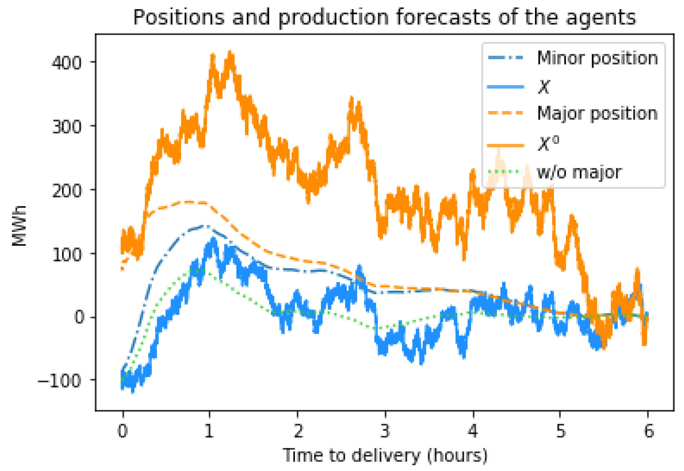
In Figure 1, we plot the major agent production forecast and common production forecast (respectively, the orange and blue solid lines) together with the equilibrium position of the major agent and the aggregate position of the minor agents given by Theorem 2 and Proposition 2 (respectively, the orange and blue dashed lines). For comparison, we also plot the aggregate position in the identical agent case (dotted green line). All of the trajectories have been computed with the same production forecasts, the same fundamental price, initial values, volatilities, and parameters, as specified in Table 1, except for the price impact coefficients of major and minor player, which differ according to model specification. In the Stackelberg game, we chose $a^0=a=0.5$ €/MWh${}^2$ and, in the homogeneous case, we kept $a=1$ €/MWh${}^2$.

We observe that the strategy in the setting of identical agents and the strategy of the minor player in the Stackelberg setting converge to the same terminal value due to the terminal penalty. However, in the Stackelberg case, the minor agent position tends to follow the one of the major player during the first part of the trading period. In the case of identical agents, the fluctuations are not as strong, since, contrary to the case when a major agent is present, the minor agents have no incentive to modify their trajectory to follow the leader. During the second half of the trading period, the minor agent position deviates further away from the one of the major agent in order to target the same terminal position as the mean field in the case of identical agents. We can argue that the strategy of the minor agent becomes more sensitive to the terminal constraint as we get closer to the delivery time: the weight of the terminal constraint in the strategy increases due to the decrease of the instantaneous trading cost.

5.3. Volatility and Price-Forecast Correlation

In this paragraph, we illustrate with simulations the effect of the presence of the major agent on the price characteristics, such as the volatility and the correlation between the price and renewable infeed forecasts. The volatility was estimated from simulated price trajectories using a kernel-based non parametric estimator of the instantaneous volatility:

$${\widehat{\sigma }}_t^2=\frac{{\sum }_{i=1}^n{K}_h(t_{i-1}-t)\Delta {\tilde{P}}_{t_{i-1}}^2}{{\sum }_{i=1}^n{K}_h(t_{i-1}-t)(t_i-t_{i-1})},$$

(26)

where $K(.)$ is the Epanechnikov kernel: $K\left(x\right)=\frac{3}{4}(1-x^2){𝟙}_{[-1,1]}\left(x\right)$ and $K_h\left(x\right)=\frac{1}{h}K\left(\frac{x}{h}\right)$. The parameter h was taken equal to $0.08$ h (≈5 min).

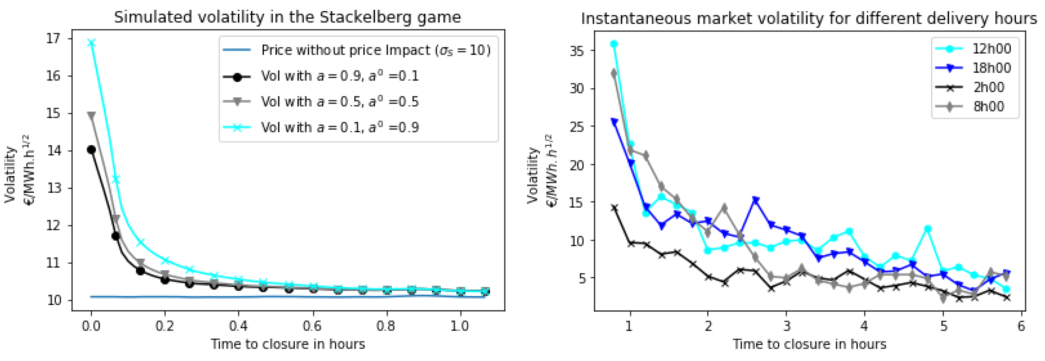
For a fixed scenario of production forecasts for the minor and major players, as drawn in Figure 1, we estimated the volatility of the simulated market price for different values of the weights $a_0$ and a assigned, respectively, to the major player and the mean field of minor players in the price impact function. We studied three different combinations of weights in order to illustrate the impact of the minor players and the major player in the game: $a^0=a=0.5$ €/MWh${}^2$, the impact of the major player and the minor players is the same; $a^0=0.9,a=0.1$ €/MWh${}^2$, the major player has a lot more impact than the minor players, and finally $a^0=0$ €/MWh${}^2$, $a=1$ €/MWh${}^2$, equivalent to a market without a major player. These weights can be seen as the respective market shares that are held by the major agent and the minor players.

Figure 2, left graph, shows the estimated volatility trajectories for the three different cases of market shares of the major agent averaged over 1000 simulations. We note that the volatility of the market price depends on the strength of impact of the major player: the greater $a^0$, the higher the volatility. A possible explanation for this phenomenon is that stronger competition in the market (when the major agent is absent or has a small market share) reduces profit opportunities in the market and the agents, therefore, trade less actively.

For comparison, we also plot, in Figure 2, right graph, the volatility estimated from empirical intraday electricity price data using the same estimator (26). This graph is taken from Féron et al. (2020). We see that the phenomenon of increasing volatility at the approach of the delivery date, which is clearly visible in the actual electricity markets, is well reproduced by our model.

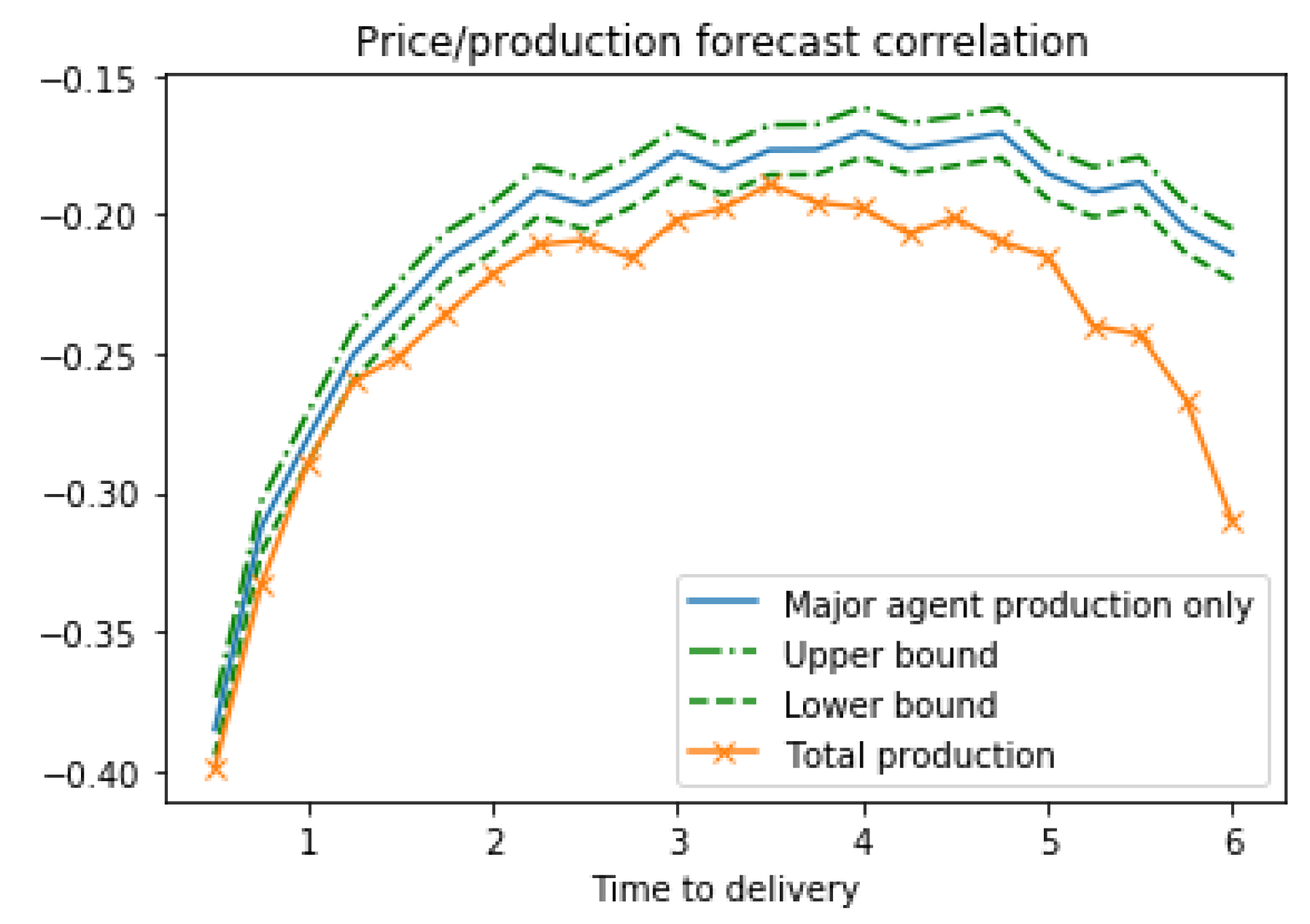
An important stylized feature of intraday market prices, observed empirically in Kiesel and Paraschiv (2017) and Féron et al. (2020), is the correlation between the price and renewable production forecasts. In Figure 3, we plotted the correlation between the increments of the market price and the increments of the renewable production forecast of the major agent as a function of time, in the market impact setting $a^0=a=0.5$ €/MWh${}^2$; as well as the correlation between the price increments and increments of the total aggregate forecast of both the major and minor players.

The correlation is computed over 15-min. increments while using the following estimator:

$${\widehat{\rho }}_t=\frac{{\sum }_{k=1}^{N_{sim}}(\Delta Y_t^k-{\overline{\Delta Y}}_t)(\Delta P_t^k-{\overline{\Delta P}}_t)}{\sqrt{{\sum }_{k=1}^{N_{sim}}{(\Delta Y_t^k-{\overline{\Delta Y}}_t)}^2{\sum }_{k=1}^{N_{sim}}{(\Delta P_t^k-{\overline{\Delta P}}_t)}^2}},$$

with $N_{sim}$ the number of simulations (we considered $N_{sim}$ = 50,000) and where $\Delta Y_t^k$ and $\Delta P_t^k=P_{t+dt}^{MF,k}-P_t^{MF,k}$ are the increments of, respectively, the forecast process and market price.

For the sake of clarity, we only draw the Monte Carlo confidence interval for the case of the correlation between the major player production and the price considered in Figure 3. A similar confidence interval was obtained for the case of total production correlation. In Figure 3, we observe that the correlation between the production forecast increments of the major agent and price is lower in absolute value than the correlation between the total production forecast increments and the price. However, the gap between the correlations diminishes as we approach the delivery time.

6. Conclusions

In this paper, we applied the theory of linear quadratic mean-field games with a major player to the analysis of intraday electricity markets. The linear quadratic setting, while allowing for obtaining explicit formulas for the equilibrium price and optimal strategies of the agents, requires one to impose a number of quite stringent assumptions on the price dynamics, such as linear market impact and quadratic hedging cost. While these assumptions have been used in a number of papers on optimal trading and order execution in financial markets, their validity in electricity markets remains to be studied. Contrary to equity and bond markets, the literature on market impact and microstructure of electricity markets is in the nascent state and we hope that our paper will motivate more in-depth analysis of this topic, and more detailed studies of order book data of electricity markets. Another important aspect of our study is the theoretical demonstration of the correlation between the renewable production forecasts and market prices. As the renewable penetration and the participation of renewable producers in intraday market increases, these correlations will become more important and they may erode the profits of the renewable producers, impeding investment flows into this important domain. Therefore, one may need to develop alternative market structures facilitating the participation of renewable producers.

References

- Aïd, René, Andrea Cosso, and Huyên Pham. 2020. Equilibrium price in intraday electricity markets. arXiv arXiv:2010.09285. [Google Scholar]
- Aïd, René, Pierre Gruet, and Huyên Pham. 2016. An optimal trading problem in intraday electricity markets. Mathematics and Financial Economics 10: 49–85. [Google Scholar] [CrossRef] [Green Version]
- Alasseur, Clémence, Imen Ben Taher, and Anis Matoussi. 2020. An extended mean field game for storage in smart grids. Journal of Optimization Theory and Applications 18: 644–70. [Google Scholar] [CrossRef] [Green Version]
- Bensoussan, Alain, Michael Chau, and Phillip Yam. 2016. Mean field games with a dominating player. Applied Mathematics & Optimization 74: 91–128. [Google Scholar]
- Bensoussan, Alain, and Sheung Chi Phillip Yam. 2019. Mean field approach to stochastic control with partial information. arXiv arXiv:1909.10287v3. [Google Scholar]
- Bouchard, Bruno, Masaaki Fukasawa, Martin Herdegen, and Johannes Muhle-Karbe. 2018. Equilibrium returns with transaction costs. Finance and Stochastics 22: 569–601. [Google Scholar] [CrossRef] [Green Version]
- Cardaliaguet, Pierre, Marco Cirant, and Alessio Porretta. 2020. Remarks on Nash equilibria in mean field game models with a major player. Proceedings of the American Mathematical Society 148: 4241–55. [Google Scholar] [CrossRef]
- Carmona, René, and François Delarue. 2018. Probabilistic Theory of Mean Field Games with Applications I. Berlin/Heidelberg: Springer. [Google Scholar]
- Carmona, Rene, and Xiuneng Zhu. 2016. A probabilistic approach to mean field games with major and minor players. The Annals of Applied Probability 26: 1535–80. [Google Scholar] [CrossRef]
- Casgrain, Philippe, and Sebastian Jaimungal. 2020. Mean-field games with differing beliefs for algorithmic trading. Mathematical Finance 30: 995–1034. [Google Scholar] [CrossRef]
- Donier, Jonathan, Julius Bonart, Iacopo Mastromatteo, and Jean-Philippe Bouchaud. 2015. A fully consistent, minimal model for non-linear market impact. Quantitative Finance 15: 1109–21. [Google Scholar] [CrossRef] [Green Version]
- Evangelista, David, and Yuri Thamsten. 2020. Finite population games of optimal execution. arXiv arXiv:2004.00790. [Google Scholar]
- Féron, Olivier, Peter Tankov, and Laura Tinsi. 2020. Price formation and optimal trading in intraday electricity markets. arXiv arXiv:2009.04786. [Google Scholar]
- Fu, Guanxing, and Ulrich Horst. 2020. Mean-field leader-follower games with terminal state constraint. SIAM Journal on Control and Optimization 58: 2078–113. [Google Scholar] [CrossRef]
- Fujii, Masaaki, and Akihiko Takahashi. 2020. A mean field game approach to equilibrium pricing with market clearing condition. CARF Working Paper CARF-F-473. arXiv arXiv:2003.03035. [Google Scholar]
- Huang, Minyi. 2010. Large-population LQG games involving a major player: The Nash certainty equivalence principle. SIAM Journal on Control and Optimization 48: 3318–53. [Google Scholar] [CrossRef]
- Huang, Minyi, Roland P. Malhamé, and Peter E. Caines. 2006. Large population stochastic dynamic games: Closed-loop McKean-Vlasov systems and the nash certainty equivalence principle. Communications in Information & Systems 6: 221–52. [Google Scholar]
- Kiesel, Rüdiger, and Florentina Paraschiv. 2017. Econometric analysis of 15-minute intraday electricity prices. Energy Economics 64: 77–90. [Google Scholar] [CrossRef] [Green Version]
- Lacker, Daniel. 2020. On the convergence of closed-loop Nash equilibria to the mean field game limit. Annals of Applied Probability 30: 1693–761. [Google Scholar] [CrossRef]
- Lasry, Jean-Michel, and Pierre-Louis Lions. 2007. Mean field games. Japanese Journal of Mathematics 2: 229–60. [Google Scholar] [CrossRef] [Green Version]
- Lasry, Jean-Michel, and Pierre-Louis Lions. 2018. Mean-field games with a major player. Comptes Rendus Mathematique 356: 886–90. [Google Scholar] [CrossRef]
- Nourian, Mojtaba, and Peter E. Caines. 2013. ϵ-Nash mean field game theory for nonlinear stochastic dynamical systems with major and minor agents. SIAM Journal on Control and Optimization 51: 3302–31. [Google Scholar] [CrossRef] [Green Version]
- Shrivats, Arvind, Dena Firoozi, and Sebastian Jaimungal. 2020. A mean-field game approach to equilibrium pricing, optimal generation, and trading in solar renewable energy certificate (srec) markets. arXiv arXiv:2003.04938. [Google Scholar]
- Tan, Zongjun, and Peter Tankov. 2018. Optimal trading policies for wind energy producer. SIAM Journal on Financial Mathematics 9: 315–46. [Google Scholar] [CrossRef] [Green Version]
Figure 1.
Demand forecasts and agents’ positions in the Stackelberg game.
Figure 2.
(Left) volatility of simulated prices for different market shares of the major agent. (Right) volatility for different delivery hours, estimated empirically from EPEX spot intraday market data of January 2017 for the Germany delivery zone.
Figure 3.
Correlation between the price increments and the major player renewable production increments vs. the correlation between the price increments and the total renewable production increments.