An Expectation-Maximization Algorithm for the Exponential-Generalized Inverse Gaussian Regression Model with Varying Dispersion and Shape for Modelling the Aggregate Claim Amount

Abstract

This article presents the Exponential–Generalized Inverse Gaussian regression model with varying dispersion and shape. The EGIG is a general distribution family which, under the adopted modelling framework, can provide the appropriate level of flexibility to fit moderate costs with high frequencies and heavy-tailed claim sizes, as they both represent significant proportions of the total loss in non-life insurance. The model’s implementation is illustrated by a real data application which involves fitting claim size data from a European motor insurer. The maximum likelihood estimation of the model parameters is achieved through a novel Expectation Maximization (EM)-type algorithm that is computationally tractable and is demonstrated to perform satisfactorily.

1. Introduction

In the recent literature, in various fields of research such as seismology, biology, genetics, econometrics and insurance, an interest has been developed in modelling right-skewed data which are dominated by large values. Similarly, from the literature in non-life insurance, such as Beirlant et al. (1992), Kleiber and Kotz (2003) and Rosenberg et al. (2007), it is well known that claim size distributions are right-skewed and heavy-tailed, meaning that it is of interest for insurance companies to quantify the risk from extreme amounts of losses. In order to keep the variation of the aggregate claim amount reasonable, an insurer usually takes out reinsurance cover for their insurance portfolio; in other words, they protect themselves against losses arising from large, excessively numerous or catastrophic claims by reinsuring large claim amounts with one or more other insurance or reinsurance companies. In other cases, unless larger claim size amounts are eliminated by reinsurance, the tail of the distribution function is of critical importance, and alternative approaches are required whenever extreme losses are under consideration. In this regard, it has become a standard practice in non-life insurance to employ heavy-tailed distributions to accommodate these extreme claim sizes.

The most well-known families of heavy-tailed distributions that have been utilized in actuarial practice for this purpose are the Generalized Inverse Gaussian (GIG) and Generalized Beta of the second kind (GB2) families. The GIG distribution, which was comprehensively explored in Jorgensen (1982) and Johnson et al. (1994), includes the Inverse Gaussian as a special case and the Gamma and Inverse Gamma distributions as limiting cases. Note that the Inverse Gamma distribution also includes some well-known distributions such as the Inverse Exponential, Inverse Chi Squared and Scaled Inverse Chi Squared distributions. The GB2 distribution includes the Burr, generalized Pareto and Pareto distributions as special cases and the Generalized Gamma (GG) distribution as a limiting case. The distributions which belong to the GB2 family have been widely used in the actuarial literature to model heavy-tailed insurance loss data for cases with and without covariate information; see, for instance, Frees et al. (2014, 2016); Frees and Valdez (2008); Hürlimann (2014); Jeong (2020); Jeong and Valdez (2020); Laudagé et al. (2019); Ramirez-Cobo et al. (2010); Shi et al. (2015); Wang et al. (2020); Yang et al. (2011), among many others.

Furthermore, it should be noted that alternative approaches have been considered in the actuarial literature to model heavy-tailed losses. Log phase-type distributions were considered in (Ahn et al. 2012; Bladt and Rojas-Nandayapa 2018; Hassan Zadeh and Stanford 2016) in the context of regression analysis. The Double-Pareto-Lognormal (DPLN) distribution was proposed in Calderín-Ojeda et al. (2017) to efficiently model large claim amounts with heavy-tail behaviors. Additionally, the use of continuous mixture distributions has been proposed as a way to capture the heavy-tailed behavior of insurance losses. In Li et al. (2020), the authors considered a new parametric family of loss distributions, termed the Generalized Log-Moyal Gamma distribution (GLMGA), which can be derived as a Gamma mixture of the Generalized Log-Moyal distribution; see Bhati and Ravi (2018). While the GLMGA distribution that they presented is a special case of the GB2 distribution, they demonstrated that it is effective in the regression modelling of large and modal loss data. In Tzougas and Karlis (2020), the authors calibrated heavy-tailed insurance losses using a class of mixed Exponential Regression models with varying dispersion. Their proposed class of models extends the setup of many well-known two parameter mixed Exponential distributions, such as the classic Exponential–Inverse Gamma—namely Pareto—, the Exponential–Inverse Gaussian (EIG) distributions and the Exponential–Lognormal (ELN) distribution, which was recently considered in Tzougas et al. (2020).

In this study, we introduce the Exponential–Generalized Inverse Gaussian (EGIG) regression model with varying dispersion and shape to approximate heavy-tailed claim sizes in non-life insurance. The probability density function (pdf) of the model is parameterized in terms of its mean, dispersion and shape parameters. This results in a more orthogonal parameterization which facilitates maximum likelihood (ML) estimation when regression specifications are allowed for the mean, dispersion and shape parameters of the EIG distribution. Furthermore, the EGIG is a very wide family which includes many well-known mixed Exponential distributions as special and limiting cases, such as the EIG, Pareto (which can be derived either as an Exponential-Gamma or as an Exponential–Inverse Gamma), Exponential–Inverse Exponential, Exponential–Inverse Chi Squared and Exponential–Scaled Inverse Chi Squared distributions, depending on the estimated values of the dispersion and shape parameters which are modelled as functions of risk factors. This can be regarded as a very useful property since, as is well known, real non-life insurance datasets are a mix of moderate and large claim amounts. In particular, the EGIG family combined with the proposed modelling framework can provide insurance companies with a useful—from a practical business point of view—tool both to model moderate losses, which correspond to the body area of the distribution, and match the varying tail behaviors of insurance losses from different risk profiles, thus leading to a better risk-adjusted classification of policyholders with similar risk characteristics. For example, suppose that an actuary empirically knows that loss amounts from the moderate-risk profile tend to follow the EIG distribution whereas loss amounts from the high-risk profile tend to follow Pareto distribution; in such cases, the use of either the EIG or the Pareto model might not be able to efficiently approximate the claim severity for the entire dataset. However, a potential distribution misspecification can affect the degree of reliability of predictions and subsequently lead to inaccurate pricing and ratemaking. The EGIG family has the substantial flexibility to overcome these deficiencies. Additionally, unlike the majority of models for insurance losses, our general approach can allow an insurer to determine the distribution of each risk class based not only on the mean parameter, which is traditionally modelled in terms of covariates, but also by using regressors on the dispersion and shaper parameters which describe the shape of the EGIG distribution. Moreover, an insurance company might not only be interested in the predictive mean of each individual claim, but also in the predictive distributions of the individual claims for more effective enterprise risk management. Finally, it is worth noting that our main contribution is to develop an Expectation-Maximization (EM)-type algorithm which exploits the stochastic mixture representation of the EGIG model to maximize its cumbersome likelihood function expressed in terms of the modified Bessel function of the third kind. Our proposed method can also remedy the computational issues which may occur by traditional direct maximization procedures since it may not be possible to obtain numerically reliable direct first and second derivatives of the Bessel function when regression structures are incorporated in its order.

The remainder of this article is organized as follows. In Section 2, we present the construction of EGIG distributions with varying dispersion and shape. Section 3 deals with the maximum likelihood (ML) estimation procedure for our proposed model via the EM algorithm. In Section 4, we describe the Motor Third Party Liability (MTPL) dataset that we use for our empirical analysis, and we provide estimation and model comparison results for the proposed model and various benchmark models. Section 5 discusses the computational issues for the implementation of the EM algorithm wich is used to fit the EGIG regression model with varying dispersion and shape. Finally, concluding remarks are given in Section 6.

2. The Exponential–Generalized Inverse Gaussian Regression Model with Varying Dispersion and Shape

Consider a non-life insurance portfolio which consists of $i=1,\infty ,n$ policyholders. We describe the average severity as $Y_i$ of policyholder i, which is well-defined when there is at least one claim. In practice, there is often no access to the individual claim severities but only to the aggregate claim amounts. Therefore, it is customary to decompose the aggregate claim amounts into two parts: frequency and severity, where the heavy-tail behavior arises from the severity part.

Suppose that, given a continuous random variable $Z_i>0$, $Y_i|Z_i$ follows an Exponential distribution with the probability density function (pdf) given by

$$f\left(y_i|Z_i=z_i\right)=\frac{e^{-\frac{y_i}{{\mu }_i{z}_i}}}{{\mu }_i{z}_i},$$

(1)

where $y_i,{\mu }_i,z_i>0$ with $\mathbb{E}\left(Y_i\right|Z_i)={\mu }_i{Z}_i$ and $Var\left(Y_i\right|Z_i)={\left({\mu }_i{Z}_i\right)}^2.$ Note that $Y_i|Z_i$ denotes the conditional distribution of claim amounts given the latent variable $Z_i$, which accounts for the unobserved heterogeneity in risks.

Let us now assume that $Z_i$ are random variables from a Generalized–Inverse Gaussian with a pdf of

$$g(z_i;{\varphi }_i;{\nu }_i)=c_i^{{\nu }_i}\left[\frac{z_i^{{\nu }_i-1}}{2K_{{\nu }_i}\left(\frac{1}{{\varphi }_i}\right)}\right]exp\left[-\frac{1}{2{\varphi }_i}\left(c_i{z}_i+\frac{1}{c_i{z}_i}\right)\right]$$

(2)

for ${\varphi }_i>0$ and $-\infty <{\nu }_i<\infty$, where $c_i=\left[K_{{\nu }_i+1}(1/{\varphi }_i)\right]{\left[K_{{\nu }_i}(1/{\varphi }_i)\right]}^{-1}$ and

$$K_{{\nu }_i}\left(\omega \right)=\underset{0}{\overset{\infty }{\int }}{\chi }^{{\nu }_i-1}exp\left[-\frac{1}{2}\omega \left(\chi +\frac{1}{\chi }\right)\right]d\chi ,$$

(3)

is the modified Bessel function of the third kind of order ${\nu }_i$ with argument $\omega$.

Note that Equation (2) is obtained from a reparameterization of the GIG distribution which was considered by Jorgensen (1982) and Johnson et al. (1994). This parameterization ensures that the model is identifiable since $\mathbb{E}\left(Z_i\right)=1$. Note also that

$$Var\left(Z_i\right)=\frac{K_{{\nu }_i+2}\left(\frac{1}{{\varphi }_i}\right)K_{{\nu }_i}\left(\frac{1}{{\varphi }_i}\right)}{K_{{\nu }_i+1}{\left(\frac{1}{{\varphi }_i}\right)}^2}-1.$$

When considering the assumptions in Equations (1) and (2), it is easy to see that the unconditional distribution of $Y_i$ will be an Exponential–Generalized Inverse Gaussian (EGIG) distribution with a pdf given by

$$f\left(y_i\right)=\frac{c_i}{{\mu }_i}{\left(1+\frac{2y_i{c}_i{\varphi }_i}{{\mu }_i}\right)}^{\frac{{\nu }_i-1}{2}}\frac{K_{{\nu }_i-1}\left(\sqrt{\frac{1}{{\varphi }_i^2}+\frac{2y_i{c}_i}{{\mu }_i{\varphi }_i}}\right)}{K_{{\nu }_i}\left(\frac{1}{{\varphi }_i}\right)}.$$

(4)

Note that if we let $\nu =-0.5$ in Equation (4), the EGIG distribution reduces to an Exponential–Inverse Gaussian (EIG) distribution. Further, the Pareto distribution can be derived as an Exponential–Gamma or as an Exponential–Inverse Gamma since both distributions are limiting cases of Equation (4), obtained by allowing ${\varphi }_i\to \infty$ for ${\nu }_i>0$ and ${\nu }_i<-1$, respectively.

To allow for the mean, dispersion and shape parameters to be modelled as functions of explanatory variables with parametric linear functional forms, we assume that

$$\begin{array}{ccc}\hfill {\mu }_i& =& exp\left({\mathbf{x}}_{1,i}^T{\mathbf{\beta }}_1\right),\hfill \end{array}$$

(5)

$$\begin{array}{ccc}\hfill {\varphi }_i& =& exp\left({\mathbf{x}}_{2,i}^T{\mathbf{\beta }}_2\right)\mathrm{and}\hfill \end{array}$$

(6)

$$\begin{array}{ccc}\hfill {\nu }_i& =& {\mathbf{x}}_{3,i}^T{\mathbf{\beta }}_3\hfill \end{array}$$

(7)

where ${\mathbf{x}}_{1,i}$, ${\mathbf{x}}_{2,i}$ and ${\mathbf{x}}_{3,i}$ are covariate vectors with dimensions $p_1\times 1$, $p_2\times 1$ and $p_3\times 1$ respectively, with ${\mathbf{\beta }}_1={\left({\beta }_{1,1},\cdots ,{\beta }_{1,p_1}\right)}^T$, ${\mathbf{\beta }}_2={\left({\beta }_{2,1},\cdots ,{\beta }_{2,p_2}\right)}^T$ and ${\mathbf{\beta }}_3={\left({\beta }_{3,1},\cdots ,{\beta }_{3,p_3}\right)}^T$ the corresponding parameter vectors, and where it is considered that the matrices ${\mathbf{X}}_1$, ${\mathbf{X}}_2$ and ${\mathbf{X}}_3$with rows given by ${\mathbf{x}}_{1,i}$, ${\mathbf{x}}_{2,i}$ and ${\mathbf{x}}_{3,i}$ respectively, are of full rank, for $i=1,\cdots ,n$.

Finally, using the moments of the Exponential and GIG distributions, one can easily find that the mean, variance, skewness and kurtosis of $Y_i$ are as follows:

$$\mathbb{E}\left(Y_i\right)=\mathbb{E}\left[\mathbb{E}\left(Y_i|Z_i\right)\right]={\mu }_i\mathbb{E}\left[Z_i\right]={\mu }_i,$$

(8)

$$\begin{array}{ccc}\hfill Var\left(Y_i\right)& =& \mathbb{E}\left[Var\left(Y_i|Z_i\right)\right]+Va{r}_{Z_i}\left[\mathbb{E}\left(Y_i|Z_i\right)\right]\hfill \\ & =& {\mu }_i^2\left[\mathbb{E}\left(Z_i^2\right)+Var\left(Z_i\right)\right]={\mu }_i^2\left[\frac{2K_{{\nu }_i+2}\left(\frac{1}{{\varphi }_i}\right)K_{{\nu }_i}\left(\frac{1}{{\varphi }_i}\right)}{K_{{\nu }_i+1}{\left(\frac{1}{{\varphi }_i}\right)}^2}-1\right],\hfill \end{array}$$

(9)

$$Skewness\left(Y_i\right)=\frac{{(Y_i-{\mu }_i)}^3}{Var{\left(Y_i\right)}^{3/2}}=\frac{6\mathbb{E}\left(Z_i^3\right)-6\mathbb{E}\left(Z_i^2\right)+2}{{\left[2\mathbb{E}\left(Z_i^2\right)-1\right]}^{3/2}},$$

(10)

$$Kurtosis\left(Y_i\right)=\frac{{(Y_i-{\mu }_i)}^4}{Var{\left(Y_i\right)}^2}=\frac{24\mathbb{E}\left(Z_i^4\right)-24\mathbb{E}\left(Z_i^3\right)+12\mathbb{E}\left(Z_i^2\right)-3}{{\left[2\mathbb{E}\left(Z_i^2\right)-1\right]}^2},$$

(11)

where $\mathbb{E}\left(Z_i^k\right)={\displaystyle \frac{K_{{\nu }_i+k}\left(\frac{1}{{\varphi }_i}\right)·K_{{\nu }_i}{\left(\frac{1}{{\varphi }_i}\right)}^k}{K_{{\nu }_i}\left(\frac{1}{{\varphi }_i}\right)·K_{{\nu }_i+1}{\left(\frac{1}{{\varphi }_i}\right)}^k}}$ for $k\in \mathbb{N}$.

One can see that the proposed regression model satisfies $Var\left(Y_i\right)={\mu }_i^2·g({\varphi }_i,{\nu }_i)$, similar to other models such as Reparametrized Birnbaum–Saunders (Santos-Neto et al. 2016), Reparametrized Slash-Half-Normal (Gómez et al. 2019), Reparametrized Extended–Exponential (Gómez et al. 2020) and Reparametrized Slash-Rayleigh (Gallardo et al. 2020) models.

3. The EM Algorithm

In this section, an Expectation-Maximization (EM) algorithm (Dempster et al. 1977; McLachlan and Krishnan 2007) is used to facilitate the maximum likelihood (ML) estimation of the EGIG regression model with a varying dispersion and shape, which was described in Section 2. Due to the inherent heavy-tail behaviors of non-life insurance claims, continuous mixture models have been widely used in the modelling of general insurance claims. However, such models tend to have complicated and highly non-convex forms of likelihood, meaning that the naïve maximization of likelihood with well-known optimization routines often suffers from computational instability. In this regard, the use of EM algorithm can be beneficial to analyze non-life data. Let $(y_i,{\mathbf{x}}_{1,\mathbf{i}},{\mathbf{x}}_{2,\mathbf{i}},{\mathbf{x}}_{3,\mathbf{i}})$, $i=1,\cdots ,n,$ be a sample of independent observations, where $y_i$ is the response variable and ${\mathbf{x}}_{1,\mathbf{i}}$, ${\mathbf{x}}_{2,\mathbf{i}}$ and ${\mathbf{x}}_{3,\mathbf{i}}$ are the vectors of covariate information with dimensions $p_1\times 1$, $p_2\times 1$ and $p_3\times 1$ respectively. Additionally, consider that the data are produced according to the EGIG model. Then, the log-likelihood of the model can be written as

$$\begin{array}{ccc}\hfill l\left(\theta \right)& =& \sum _{i=1}^n\left[log\left(c_i\right)-log\left({\mu }_i\right)+\left(\frac{{\nu }_i-1}{2}\right)log\left(1+\frac{2y_i{c}_i{\varphi }_i}{{\mu }_i}\right)\right.\hfill \\ & & \left.+log\left(K_{{\nu }_i-1}\left(\sqrt{\frac{1}{{\varphi }_i^2}+\frac{2y_i{c}_i}{{\mu }_i{\varphi }_i}}\right)\right)-log\left(K_{{\nu }_i}\left(\frac{1}{{\varphi }_i}\right)\right)\right],\hfill \end{array}$$

(12)

where $\mathbf{\theta }={\left({\mathbf{\beta }}_1^T,{\mathbf{\beta }}_2^T,{\mathbf{\beta }}_3^T\right)}^T$ is the vector of the parameters.

The direct maximization of the above function with respect to the vector of parameters $\mathbf{\theta }$ is complicated to calculate when regression structures are allowed for the mean, dispersion and shape parameters since it would be necessary to differentiate the last two terms in Equation (12) with respect to ${\mathbf{\beta }}_1,{\mathbf{\beta }}_2$ and ${\mathbf{\beta }}_3$, respectively.

On the other hand, the ML estimation of the model can be achieved via an EM-type algorithm which, as demonstrated in Frangos and Karlis (2004), Tzougas et al. (2020) and Tzougas and Karlis (2020), is specifically tailored to ML estimation for mixed Exponential models since their stochastic mixture representation involving a non-observable random variable, denoted by $z_i$ herein, can be regarded to produce missing data. In the case of the EGIG model, if one augments the unobserved data $z_i$ to the observed data $(y_i,{\mathbf{x}}_{1,\mathbf{i}},{\mathbf{x}}_{2,\mathbf{i}},{\mathbf{x}}_{3,\mathbf{i}})$, for $i=1,\cdots ,n$, then the complete data log-likelihood factorizes into two parts as follows:

$$\begin{array}{ccc}\hfill l_c\left(\mathbf{\theta }\right)& \propto & l_c\left({\mathbf{\beta }}_1\right)+l_c\left({\mathbf{\beta }}_2,{\mathbf{\beta }}_3\right),\hfill \\ \hfill l_c\left({\mathbf{\beta }}_1\right)& =& \sum _{i=1}^n\left[-\frac{y_{it}}{{\mu }_i{z}_i}-log\left({\mu }_i\right)\right],\hfill \\ \hfill l_c\left({\mathbf{\beta }}_2,{\mathbf{\beta }}_3\right)& =& \sum _{i=1}^n\left[{\nu }_{i}log\left(c_i\right)+\left({\nu }_i-1\right)log\left(z_i\right)-log\left(K_{{\nu }_i}\left(\frac{1}{{\varphi }_i}\right)\right)-\frac{1}{2{\varphi }_i}\left(c_i{z}_i+\frac{1}{c_i{z}_i}\right)\right].\hfill \end{array}$$

(13)

In what follows, at the E-Step of the algorithm, it is necessary to compute the Q-function, which is the conditional expectation of the complete log-likelihood data, while the M-Step consists of maximizing the Q-function with respect to $\mathbf{\theta }$. The Q-function is proportional to the sum of the terms which involve the regression coefficients ${\mathbf{\beta }}_1^{\left(r\right)}$, ${\mathbf{\beta }}_2^{\left(r\right)}$ and ${\beta }_{\mathbf{3}}^{\left(r\right)}$:

$$\begin{array}{ccc}\hfill Q\left(\mathbf{\theta };{\mathbf{\theta }}^{\left(r\right)}\right)& \equiv & \mathbb{E}\left(l_c\left(\mathbf{\theta }\right)|k_i;{\mathbf{\theta }}^{\left(r\right)}\right)\propto \hfill \\ & \propto & \sum _{i=1}^n\left[-\frac{y_i\mathbb{E}\left[\frac{1}{z_i}|y_i;{\mathbf{\theta }}^{\left(r\right)}\right]}{{\mu }_i^{\left(r\right)}}-log\left({\mu }_i^{\left(r\right)}\right)\right]+\sum _{i=1}^n\left[{\nu }_i^{\left(r\right)}log\left(c_i^{\left(r\right)}\right)\right.\hfill \\ & & +\left({\nu }_i^{\left(r\right)}-1\right)\mathbb{E}\left[log\left(z_i\right)|y_i;{\mathbf{\theta }}^{\left(r\right)}\right]-log\left(K_{{\nu }_i^{\left(r\right)}}\left(\frac{1}{{\varphi }_i^{\left(r\right)}}\right)\right)\hfill \\ & & \left.-\frac{1}{2{\varphi }_i^{\left(r\right)}}\left(c_i^{\left(r\right)}\mathbb{E}\left[z_i|y_i;{\mathbf{\theta }}^{\left(r\right)}\right]+\frac{\mathbb{E}\left[\frac{1}{z_i}|y_i;{\mathbf{\theta }}^{\left(r\right)}\right]}{c_i^{\left(r\right)}}\right)\right],\hfill \end{array}$$

(14)

where ${\mathbf{\theta }}^{\left(r\right)}$ is the estimate of $\mathbf{\theta }$ at the rth iteration in the E-step of our EM type algorithm, where ${\mu }_i^{\left(r\right)}=exp\left({\mathbf{x}}_{1,i}^T{\mathbf{\beta }}_1^{\left(r\right)}\right)$, ${\varphi }_i^{\left(r\right)}=exp\left({\mathbf{x}}_{2,i}^T{\mathbf{\beta }}_2^{\left(r\right)}\right)$ and ${\nu }_i^{\left(r\right)}={\mathbf{x}}_{3,i}^T{\mathbf{\beta }}_3^{\left(r\right)}$ and $c_i^{\left(r\right)}=\left[K_{{\nu }_i^{\left(r\right)}+1}(1/{\varphi }_i^{\left(r\right)})\right]{\left[K_{{\nu }_i^{\left(r\right)}}(1/{\varphi }_i^{\left(r\right)})\right]}^{-1}$. At this point, we would like to call attention to the fact that if $y_i\sim$ Exponential$\left({\mu }_i{z}_i\right)$ distribution and $z_i\sim$ GIG $\left(\frac{c_i}{{\varphi }_i},\frac{1}{c_i{\varphi }_i},{\nu }_i\right)$ distribution, then, applying Bayes theorem, one can find that the posterior distribution of $z_i|y_i;\mathbf{\theta }$ is a GIG distribution with a pdf

$$f\left(z_i|y_i;\mathbf{\theta }\right)=\frac{{\left(\frac{a_i}{b_i}\right)}^{\frac{p_i}{2}}}{2K_{p_i}\left(\sqrt{a_i{b}_i}\right)}{z}_i^{p_i-1}exp\left[-\frac{1}{2}\left(a_i{z}_i+\frac{b_i}{z_i}\right)\right],$$

(15)

where $a_i=\frac{c_i}{{\varphi }_i}>0$, $b_i=\frac{1}{c_i{\varphi }_i}+\frac{2y_i}{{\mu }_i}>0$ and $p_i={\nu }_i-1\in \mathcal{R}$ and where ${\mu }_i$, ${\varphi }_i$ and ${\nu }_i$ are given by Equations (5)–(7), respectively. The above result will enable us to calculate the conditional expectations $\mathbb{E}\left[z_i|y_i;{\mathbf{\theta }}^{\left(r\right)}\right]$, $\mathbb{E}\left[\frac{1}{z_i}|y_i;{\mathbf{\theta }}^{\left(r\right)}\right]$ and $\mathbb{E}\left[log\left(z_i\right)|y_i;{\theta }^{\left(r\right)}\right]$ which are involved in Equation (14) and hence are required at the E-Step of the EM algorithm. Furthermore, the following well-known relationships between the modified Bessel functions of the third kind of different orders—see, for example, Abramowitz and Stegun (1965)—will be useful for implementing the M-step of the EM algorithm.

$$\begin{array}{c}\hfill K_{\nu }\left(\omega \right)=K_{\nu -2}\left(\omega \right)+\frac{2(\nu -1)}{\omega }{K}_{\nu -1}\left(\omega \right)\end{array}$$

(16)

$$\begin{array}{c}\hfill \frac{\partial K_{\nu }\left(z\right)}{\partial \omega }=\frac{\nu }{\omega }{K}_{\nu }\left(\omega \right)-K_{\nu +1}\left(\omega \right)\end{array}$$

(17)

The EM-type algorithm for the EGIG regression model with a varying dispersion and shape can be formally described as follows.

• E-Step: Given the current estimates ${\mathbf{\theta }}^{\left(r\right)}$ taken from the rth iteration, calculate for all $i=1,\cdots ,n$ the pseudo-values

  $$\begin{array}{c}\hfill w_{1,i}=\mathbb{E}\left[z_i|y_i;{\mathbf{\theta }}^{\left(r\right)}\right]=\sqrt{\frac{b^{\left(r\right)}}{a^{\left(r\right)}}}\frac{K_{p_i^{\left(r\right)}+1}\left(\sqrt{a^{\left(r\right)}{b}^{\left(r\right)}}\right)}{K_{p_i^{\left(r\right)}}\left(\sqrt{a^{\left(r\right)}{b}^{\left(r\right)}}\right)},\end{array}$$

  (18)

  $$\begin{array}{c}\hfill w_{2,i}=\mathbb{E}\left[\frac{1}{z_i}|y_i;{\mathbf{\theta }}^{\left(r\right)}\right]=\sqrt{\frac{a^{\left(r\right)}}{b^{\left(r\right)}}}\frac{K_{p_i^{\left(r\right)}-1}\left(\sqrt{a^{\left(r\right)}{b}^{\left(r\right)}}\right)}{K_{p_i^{\left(r\right)}}\left(\sqrt{a^{\left(r\right)}{b}^{\left(r\right)}}\right)}\end{array}$$

  (19)

  and

  $$w_{3,i}=\mathbb{E}\left[log\left(z_i\right)|y_i;{\mathbf{\theta }}^{\left(r\right)}\right]=log\left(\sqrt{\frac{b^{\left(r\right)}}{a^{\left(r\right)}}}\right)+\frac{\partial K_{p_i^{\left(r\right)}}\left(\sqrt{a^{\left(r\right)}{b}^{\left(r\right)}}\right)/\partial p_i^{\left(r\right)}}{K_{p_i^{\left(r\right)}}\left(\sqrt{a^{\left(r\right)}{b}^{\left(r\right)}}\right)},$$

  (20)

  where $a_i^{\left(r\right)}=\frac{c_i^{\left(r\right)}}{{\varphi }_i^{\left(r\right)}}>0$, $b_i^{\left(r\right)}=\frac{1}{c_i^{\left(r\right)}{\varphi }_i^{\left(r\right)}}+\frac{2y_i}{{\mu }_i^{\left(r\right)}}>0$ and $p_i^{\left(r\right)}={\nu }_i^{\left(r\right)}-1$.
  In this study, Equations (18)–(20) are evaluated based on the function Egig1 within the R package ghyp, which was recently created by Breymann et al. (2020).
• M-Step: Using the pseudo-values $w_{1,i}$, $w_{2,i}$ and $w_{3,i}$ from the E-Step and the Newton–Raphson algorithm three times find the maximum global point ${\mathbf{\theta }}^{\left(r+1\right)}$ of the $Q-$function; i.e., obtain the updated estimates ${\mathbf{\beta }}_1^{\left(r+1\right)}$, ${\mathbf{\beta }}_2^{\left(r+1\right)}$ and ${\mathbf{\beta }}_3^{\left(r+1\right)}$.
  Firstly, differentiate the $Q-$function with respect to ${\mathbf{\beta }}_1$:

  $$h_1\left({\mathbf{\beta }}_1\right)=\frac{\partial Q\left(\mathbf{\theta };{\mathbf{\theta }}^{\left(r\right)}\right)}{\partial {\beta }_{1,j}},$$

  (21)

  and

  $$H_1\left({\mathbf{\beta }}_1\right)=\frac{{\partial }^{2}Q\left(\mathbf{\theta };{\mathbf{\theta }}^{\left(r\right)}\right)}{\partial {\beta }_{1,j}\partial {\beta }_{1,j}^T},$$

  (22)

  for $i=1,\cdots ,n$ and $j=1,\cdots ,p_1$.
  Then, the iterative procedure for the Newton–Raphson algorithm for ${\mathbf{\beta }}_1$ is as follows:

  $${\mathbf{\beta }}_1^{\left(r+1\right)}\equiv {\mathbf{\beta }}_1^{\left(r\right)}-{\left[H_1\left({\mathbf{\beta }}_1^{\left(r\right)}\right)\right]}^{-1}{h}_1\left({\mathbf{\beta }}_1^{\left(r\right)}\right).$$

  (23)
  Secondly, differentiate the $Q-$function with respect to ${\mathbf{\beta }}_2$:

  $$\begin{array}{ccc}\hfill h_2\left({\mathbf{\beta }}_2\right)& =& \frac{\partial Q\left(\mathbf{\theta };{\mathbf{\theta }}^{\left(r\right)}\right)}{\partial {\beta }_{2,j}},\hfill \end{array}$$

  (24)

  $$\begin{array}{ccc}\hfill H_2\left({\mathbf{\beta }}_2\right)& =& \frac{{\partial }^{2}Q\left(\mathbf{\theta };{\mathbf{\theta }}^{\left(r\right)}\right)}{\partial {\beta }_{2,j}\partial {\beta }_{2,j}^T},\hfill \end{array}$$

  (25)

  for $i=1,\cdots ,n$ and $j=1,\cdots ,p_2$ Then, the Newton–Raphson iterative algorithm for ${\mathbf{\beta }}_2$ is as follows:

  $${\mathbf{\beta }}_2^{\left(r+1\right)}\equiv {\mathbf{\beta }}_2^{\left(r\right)}-{\left[H_2\left({\mathbf{\beta }}_2^{\left(r\right)}\right)\right]}^{-1}{h}_2\left({\mathbf{\beta }}_2^{\left(r\right)}\right),$$

  (26)

  for $i=1,\cdots ,n$ and $j=1,\cdots ,p_{2.}$
  Finally, differentiate the $Q-$function with respect to ${\mathbf{\beta }}_3$:

  $$\begin{array}{ccc}\hfill h_3\left({\mathbf{\beta }}_3\right)& =& \frac{\partial Q\left(\mathbf{\theta };{\mathbf{\theta }}^{\left(r\right)}\right)}{\partial {\beta }_{3,j}},\hfill \end{array}$$

  (27)

  and

  $$\begin{array}{ccc}\hfill H_3\left({\mathbf{\beta }}_3\right)& =& \frac{{\partial }^{2}Q\left(\mathbf{\theta };{\mathbf{\theta }}^{\left(r\right)}\right)}{\partial {\beta }_{3,j}\partial {\beta }_{3,j}^T},\hfill \end{array}$$

  (28)

  for $i=1,\cdots ,n$ and $j=1,\cdots ,p_3$.
  Then, the iterative procedure for the Newton–Raphson algorithm for ${\mathbf{\beta }}_3$ is as follows:

  $${\mathbf{\beta }}_3^{\left(r+1\right)}\equiv {\mathbf{\beta }}_3^{\left(r\right)}-{\left[H_3\left({\mathbf{\beta }}_3^{\left(r\right)}\right)\right]}^{-1}{h}_3\left({\mathbf{\beta }}_3^{\left(r\right)}\right).$$

  (29)
  Note that the expressions for $h_1\left({\mathbf{\beta }}_1\right)$ and $H_1\left({\mathbf{\beta }}_1\right)$, $h_2\left({\mathbf{\beta }}_2\right)$ and $H_2\left({\mathbf{\beta }}_2\right)$, and $h_3\left({\beta }_3\right)$ and $H_3\left({\beta }_3\right)$ which are involved in the M-step of the algorithm are given in Appendix A.

4. Empirical Analysis

We conducted an empirical analysis using a sample of claim severity data, which was randomly selected from a pool of 4,381,022 motor third-party liability (MTPL) insurance policies observed during the year 2017 from a major European insurance company. The sample comprised insured parties with complete records; i.e., with the availability of all a priori rating variables under consideration, and with at least one reported accident. There were 9525 observations that met our criteria. The response variable was the cost of claims at fault registered for each insured vehicle in the dataset, and the a priori rating variables we employed were the years that the policyholder had been with the company (YC), the age of their car (AC) and the horsepower (HP) of their car. Furthermore, an exploratory analysis was carried out in order to accurately select the subset of explanatory variables with the highest predictive power for the costs of claims. Additionally, in light of the heterogeneity that existed within the portfolio, we grouped the levels of each a priori rating variable with respect to risk profiles with a similar claim severity. This enabled us to achieve ratemaking accuracy and balance the homogeneity and sufficiency of the volume of data in each cell in order to provide credible patterns. This was necessary, since, under the proposed modelling framework, the mean, dispersion and shape parameters of the Exponential–Generalized Inverse Gaussian (EGIG) distribution were modelled in terms of covariates.

• The variable YC consisted of three categories of policyholders: those who had been with the company for “less than 4 years” (C1), “between 4 to 8 years” (C2) and “more than 8 years” (C3).
• The variable AC consisted of three categories of cars: those with an age “between 0 to 7 years” (C1), “between 7 to 14 years” (C2) and “greater than 14 years” (C3).
• The variable HP consisted of three categories of cars: those with a HP of “0-1400 cc” (C1), “1400–1800 cc” (C2) and “greater than 1800 cc” (C3).

Table 1. Descriptive statistics of claim severities—size of the different categories of the explanatory variables.

Statistic	Claim Severities	Years with the Company (YC)		Age of the Car (AC)		Horsepower of the Car (HP)
Minimum	75	C1:	2381	C1:	2737	C1:	3510
Median	3211	C2:	2432	C2:	1242	C2:	4064
Mean	8638	C3:	4712	C3:	5546	C3:	1951
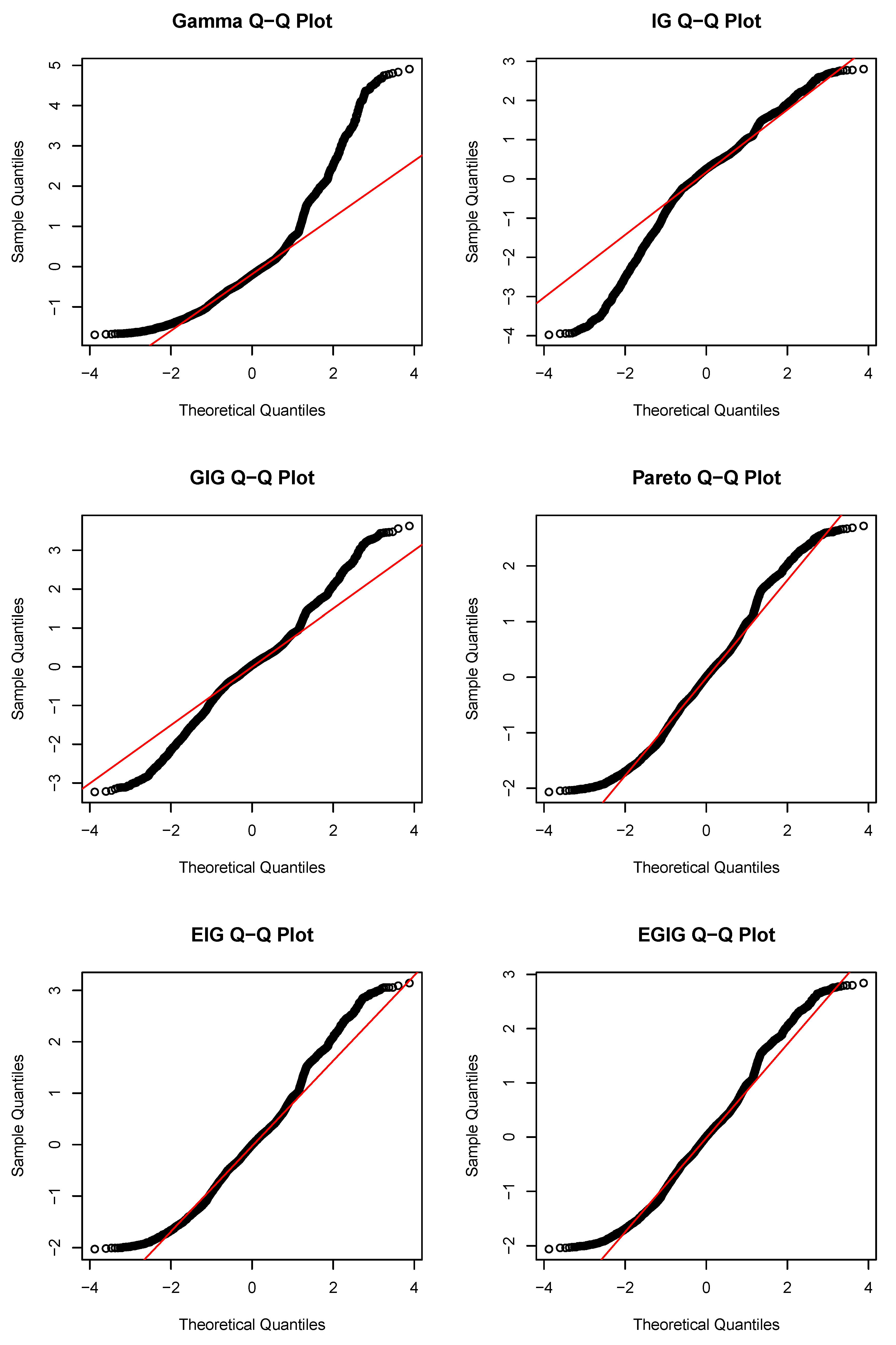
Maximum	$183,721$		−		−		−

shows brief descriptive statistics for claim severities along with the number of observations in each category of the three explanatory variables.

To assess the novelty of the proposed method, the following models were considered as benchmarks besides the proposed model. Note that for all models below ${\mu }_i$, ${\varphi }_i$ and ${\nu }_i$ are defined by Equations (5)–(7).

• Gamma (GA):

  $$f\left(y_i\right)=\frac{1}{\Gamma \left({\varphi }_i^{-2}\right){\left({\mu }_i{\varphi }_i^2\right)}^{{\varphi }_i^{-2}}}{y}_i^{{\varphi }_i^{-2}-1}{e}^{-\frac{y_i}{{\mu }_i{\varphi }_i^2}},$$

  (30)

  where $\mathbb{E}\left(Y_i\right)={\mu }_i$ and $Var\left[Y_i\right]={\mu }_i^2{\varphi }_i^2$.
• Inverse Gaussian (IG):

  $$f\left(y_i\right)={\displaystyle \sqrt{\frac{1}{2\pi {\varphi }_i^2{y}_i^3}}exp\left[-\frac{{(y_i-{\mu }_i)}^2}{2{\mu }_i^2{\varphi }_i^2{y}_i}\right]},$$

  (31)

  where $\mathbb{E}\left(Y_i\right)={\mu }_i$ and $Var\left[Y_i\right]={\mu }_i^3{\varphi }_i^2$.
• Pareto:

  $$f\left(y_i\right)=\frac{{\varphi }_i{\left[({\varphi }_i-1){\mu }_i\right]}^{{\varphi }_i}}{{[y_i+({\varphi }_i-1){\mu }_i]}^{{\varphi }_i+1}},$$

  (32)

  where $\mathbb{E}\left(Y_i\right)={\mu }_i$, and $Var\left[Y_i\right]={\mu }_i^2\left({\displaystyle \frac{{\varphi }_i}{{\varphi }_i-2}}\right)$ exists only if ${\varphi }_i>2$.
• Exponential–Inverse Gaussian (EIG):

  $$f\left(y_i\right)=\frac{{\varphi }_{i}exp\left[-{\varphi }_i\left(\sqrt{{\varphi }_i^2+\frac{2y_i}{{\mu }_i}}-{\varphi }_i\right)\right]\left({\varphi }_i\sqrt{{\varphi }_i^2+\frac{2y_i}{{\mu }_i}}+1\right)}{{\mu }_i{\left({\varphi }_i^2+\frac{2y_i}{{\mu }_i}\right)}^{3/2}},$$

  (33)

  where $\mathbb{E}\left(Y_i\right)={\mu }_i$ and $Var\left[Y_i\right]={\mu }_i^2\left({\displaystyle \frac{2}{{\varphi }_i^2}}+1\right)$.
• GIG:

  $$f\left(y_i\right)={\left(\frac{c_i}{{\mu }_i}\right)}^{{\nu }_i}\left[\frac{y_i^{{\nu }_i-1}}{2K_{{\nu }_i}\left(\frac{1}{{\varphi }_i}\right)}\right]exp\left[-\frac{1}{2{\varphi }_i}\left(\frac{c_i{y}_i}{{\mu }_i}+\frac{{\mu }_i}{c_i{y}_i}\right)\right]$$

  (34)

  where $\mathbb{E}\left(Y_i\right)={\mu }_i$, $Var\left[Y_i\right]={\mu }_i^2\left[\frac{K_{{\nu }_i+2}\left(\frac{1}{{\varphi }_i}\right)K_{{\nu }_i}\left(\frac{1}{{\varphi }_i}\right)}{K_{{\nu }_i+1}{\left(\frac{1}{{\varphi }_i}\right)}^2}-1\right]$ and $c_i=\left[K_{{\nu }_i+1}(1/{\varphi }_i)\right]$${\left[K_{{\nu }_i}(1/{\varphi }_i)\right]}^{-1}$.
• EGIG: Defined by Equation (4).

Table 2. Estimation of regression coefficients. GA: Gamma; IG: Inverse Gaussian; EIG: Exponential–Inverse Gaussian; GIG: Generalized Inverse Gaussian; EGIG: Exponential–Generalized Inverse Gaussian; AIC: Akaike information criterion: BIC: Bayesian information criterion.

	GA		IG		Pareto		EIG		GIG			EGIG
	${\mathbf{\beta }}_{\mathbf{1}}$	${\mathbf{\beta }}_{\mathbf{2}}$	${\mathbf{\beta }}_{\mathbf{1}}$	${\mathbf{\beta }}_{\mathbf{2}}$	${\mathbf{\beta }}_{\mathbf{1}}$	${\mathbf{\beta }}_{\mathbf{2}}$	${\mathbf{\beta }}_{\mathbf{1}}$	${\mathbf{\beta }}_{\mathbf{2}}$	${\mathbf{\beta }}_{\mathbf{1}}$	${\mathbf{\beta }}_{\mathbf{2}}$	${\mathbf{\beta }}_{\mathbf{3}}$	${\mathbf{\beta }}_{\mathbf{1}}$	${\mathbf{\beta }}_{\mathbf{2}}$	${\mathbf{\beta }}_{\mathbf{3}}$
(Intercept)	9.124	0.2796	9.123	−3.573	9.3372	0.3649	9.1016	−0.2908	9.1295	0.8555	−0.0889	9.1357	1.1978	−1.2825
	(0.0367)	(0.0137)	(0.0732)	(0.0163)	(0.1057)	(0.0585)	(0.0531)	(0.0484)	(0.047)	(0.0221)	(0.0265)	(0.062)	(0.1059)	(0.1266)
YCC2	−0.0047		−0.0009		0.0284		0.0204		0.0083			0.0262
	(0.0396)		(0.0783)		(0.0457)		(0.0461)		(0.0416)			(0.0409)
YCC3	−0.0018		0.0003		0.0098		0.0068		−0.0146			0.0085
	(0.0327)		(0.0645)		(0.0379)		(0.0382)		(0.0344)			(0.036)
ACC2	−0.0304	−0.0249	−0.0307	−0.0574	−0.1395	0.1115	−0.0475	0.0942	−0.032	−0.0604		−0.0461	−0.2767
	(0.0441)	(0.0204)	(0.0861)	(0.0243)	(0.1183)	(0.083)	(0.0662)	(0.0712)	(0.0594)	(0.0321)		(0.0813)	(0.322)
ACC3	−0.0625	−0.0149	−0.0626	−0.0057	−0.1316	0.0673	−0.0736	0.061	−0.0624	−0.0289		−0.0621	−0.1342
	(0.0305)	(0.0139)	(0.061)	(0.0165)	(0.0957)	(0.0596)	(0.0468)	(0.0488)	(0.0415)	(0.0221)		(0.0673)	(0.289)
HPC2	−0.0253	−0.0241	−0.0264	−0.0207	−0.0891	0.0918	−0.0251	0.081	−0.0272	−0.0316	0.0697	−0.0317	−0.1126	−0.1434
	(0.0302)	(0.0137)	(0.06)	(0.0163)	(0.0848)	(0.0566)	(0.0454)	(0.048)	(0.0407)	(0.0218)	(0.0368)	(0.0573)	(0.3683)	(0.1807)
HPC3	−0.0359	−0.011	−0.0374	−0.019	−0.0835	0.0409	−0.04	0.024	−0.0436	−0.0298	−0.0202	−0.0456	−0.1193	0.0167
	(0.0393)	(0.0168)	(0.0776)	(0.02)	(0.1103)	(0.0693)	(0.0585)	(0.0585)	(0.0528)	(0.0272)	(0.0454)	(0.0738)	(0.4718)	(0.2644)
Deviance		189,663		188,082		187,316		187,375			187,345			187,300
AIC		189,687		188,106		187,340		187,399			187,375			187,330
BIC		189,773		188,192		187,426		187,485			187,483			187,438

presents the estimated regression coefficients and the corresponding standard errors in parentheses for the GA, IG, EIG, Pareto, GIG and EGIG models, which are given by Equations (4) and (30)–(34), respectively. Furthermore, with respect to the model selection, Table 2 depicts the deviance (DEV), Akaike information criterion (AIC) and the Bayesian information criterion (BIC) values for all of the fitted models. At this point, it should be mentioned that we used a model selection technique similar to the one considered in Tzougas and Karlis (2020). In particular, we started by selecting the best predictor for the parameter ${\mu }_i$ of each claim severity model. This was done by adding all three explanatory variables—YC, AC and HP—and testing whether the exclusion of each one would result in lower DEV, AIC and BIC values. Subsequently, we continued by testing which explanatory variable between those used in parameter ${\mu }_i$ would lead to a further decrease of the DEV, AIC and BIC values when inserted into parameters ${\varphi }_i$ and ${\nu }_i$ for each claim severity model. Additionally, if different parameter specifications for the same claim severity model resulted in small discrepancies in the DEV, AIC and BIC values, we opted for the simpler models with fewer predictors for ${\varphi }_i$ and ${\nu }_i$ in order to avoid overfitting. In the above respect, as we can observe from Table 2, the variables YC, AC and HP were in the model equation for ${\mu }_i$, the variables AC and HP were in the model equation for ${\varphi }_i$ in the case of all claim severity models, and the variable HP was in the model equation for ${\nu }_i$ in the case of the GIG and EGIG models. Furthermore, we see that the magnitudes and signs of the estimated regression coefficients of the variables YC, AC and HP for ${\mu }_i$ were almost identical across all claim severity models, whereas the values and the effects (positive and/or negative) of the estimated regression coefficients of the variables AC and HP for ${\varphi }_i$ and the variable HP for ${\nu }_i$ varied among the claim severity models. In the following, we see that, due to this discrepancy, the claim severity models were better to compare in terms of their standard deviation values rather than their mean values, which are usually considered in risk classification literature. Additionally, regarding the comparison of the alternative claim severity models based on the model selection criteria, as is well known, a model noticeably outperforms its competitor if the difference in their log-likelihoods exceeds five, corresponding to a difference in their respective AIC values of more than 10 and to a difference in their BIC values of more than five; see Burnham and Anderson (2002) and Raftery (1995) respectively. Thus, as we can see from Table 2, the EGIG model gives the best fit. Finally, the normalized randomized quantile residuals—see Dunn and Smyth (1996)—were used as a graphical tool to help us assess the adequacy of the fit of the competing models. The normalized randomized quantile residuals for these claim severity regression models are defined as ${\widehat{r}}_i={\Phi }^{-1}\left(u_i\right),$ where ${\Phi }^{-1}$ is the inverse cumulative distribution function of a standard normal distribution and where $u_i=F_i\left(y_i\right|{\mathbf{\theta }}^{\left(r+1\right)})$  where $F_i$ is the cumulative distribution function estimated for the ith insured and where ${\mathbf{\theta }}^{\left(r+1\right)}$ is the vector of the estimated model parameters after the EM algorithm has reached the global maximum and $y_i$ is the corresponding observation. The claim severity model fit could be investigated via the usual quantile–quantile plots. In particular, if the data indeed followed the assumed claim severity distribution, then the residual on the quantile–quantile plot would fall approximately on a straight line. From Figure 1, we observe that the mixed Exponential models provided better assumptions than the GA, IG and GIG models since their residuals were close to the diagonal line and also yielded a better performance than that close to the right tail of the claim size distribution. Therefore, as an overall conclusion, it is reasonable to suggest the use of the EGIG model for modelling claim severity in our data set.

Table 3. Summary of calculated premium and standard deviation.

		GA	IG	Pareto	EIG	GIG	EGIG
	Min.	8275.03	8283.31	9032.57	8006.52	8175.75	8333.18
	1st Quartile	8387.38	8385.47	9194.33	8182.25	8364.69	8521.95
Premium	Median	8602.25	8609.89	9953.20	8389.93	8566.93	8721.97
	Mean	8638.44	8638.59	9918.75	8458.18	8637.75	8796.48
	3rd Quartile	8882.80	8886.44	10,487.38	8748.00	8845.74	8991.19
	Max.	9173.15	9166.15	11,679.61	9154.69	9299.66	9527.14
	Min.	10,638.09	20,568.32	NA	15,619.10	10,786.21	20,367.60
	1st Quartile	10,669.09	20,954.85	NA	15,940.62	10,990.80	21,494.80
Standard	Median	11,209.61	22,214.70	NA	17,011.01	11,481.16	22,747.08
Deviation	Mean	11,153.58	22,033.36	NA	16,963.28	11,450.85	23,202.42
	3rd Quartile	11,522.13	22,841.89	NA	17,709.45	11,772.04	24,269.96
	Max.	12,132.53	24,635.57	NA	19,587.28	12,641.57	27,655.98

provides the summary of the calculated premiums (Panel A) and standard deviations (Panel B) under each model. From Table 3, we observe that, as previously mentioned, the premiums are almost identical under different distributional assumptions, whereas noticeable discrepancies can be found in the standard deviation values of the claim severity models. Furthermore, we see that the GA model, a usual choice for claim severity, results in the smallest values of the estimated standard deviation, which can be partially explained by the failure of the model to capture the heavy-tail behavior of observed data, as shown in Figure 1. We also notice that the standard deviation cannot be computed for the Pareto model because the maximum value of ${\varphi }_i$ under the Pareto model is at most $1.765$. Therefore, the heavy-tail behavior of the data can be captured by the Pareto model at the expense of losing the feasibility of computing variance. On the other hand, the use of the EGIG model allows us to not only capture the heavy-tail behavior but also to quantify the dispersion at an individual level. Thus, the simultaneous modelling of ${\mu }_i,{\varphi }_i$ and ${\nu }_i$ of the EGIG model in terms of the a priori rating of variables is justified because it enables us to use all the available information in the estimation of the variance of the claim severity, which is an important risk measure as it can provide a measure of the uncertainty regarding different risk classes of policyholders, leading to a better risk classification.

5. Computational Aspects

This subsection discusses the computational issues related to the ML estimation of the EGIG regression model with varying dispersion and shape via the EM algorithm which was presented in Section 3. A rather strict stopping criterion was used, and the EGIG model required quite a large number of EM iterations to converge. In particular, the algorithm iterated between the E and the M-steps until the relative change in the log-likelihood between two successive iterations was smaller than ${10}^{-12}$. Also, it should be noted that the choice of sensible initial values for the vectors of regression coefficients ${\mathbf{\beta }}_1,{\mathbf{\beta }}_2$ and ${\mathbf{\beta }}_3$ can influence the speed of convergence of the EM and its ability to locate the global maximum. We obtained good starting values for ${\mathbf{\beta }}_1$ by fitting the Exponential regression. Alternatively, the initial values could be obtained based on the data as follows: (i) calculating $\mathbb{E}\left(Y_i\right)={\mu }_i,$ with $i=1,\cdots ,n$—see Equation (8)—for the different risk classes, which could be formed by dividing the portfolio into clusters defined by the combinations of the available explanatorily variables and (ii) assuming a log-link function for ${\mu }_i$—see Equation (5)—and solving Equation (5) with respect to ${\mathbf{\beta }}_1$, since, under the parameterization method we adopted, the mean is an explicit parameter of the EGIG model.

Furthermore, meaningful initial values for the regression parameters ${\mathbf{\beta }}_2$ and ${\mathbf{\beta }}_{\mathbf{3}}$ were obtained by (i) calculating $Var\left(Y_i\right)$, $skewness\left(Y_i\right)$ and $kurtosis\left(Y_i\right)$—see Equations (9)–(11)—for the different risk classes based on all observations $i=1,\cdots ,n$, (ii) by calculating $\mathbb{E}\left(Y_i\right)={\mu }_i$ with $i=1,\cdots ,n$ for the different risk classes (or alternatively computing ${\mu }_i$, based on the initial values for ${\mathbf{\beta }}_1$ and on the log-link function given by Equation (5)) and using the log-link function for ${\varphi }_i$—see Equation (6)—and the identity function for ${\nu }_i$—see Equation (7)—and so we found the values which satisfied Equations (9)–(11). Additionally, the standard errors of the regression coefficients were obtained using the standard method in Louis (1982). All computing was performed using the programming language R. Finally, the EIG and Pareto regression models with varying dispersion were fitted using the EM algorithm, which was considered in Tzougas and Karlis (2020), while the GA and IG regression models with varying dispersion and the GIG regression model with varying dispersion and shape were estimated using the generalized additive models for the location, scale and shape (GAMLSS) package in R; see Stasinopoulos et al. (2008).

6. Concluding Remarks

In this paper, we proposed an EM-type algorithm to estimate the parameters of the EGIG regression model with varying dispersion and shape. The Exponential–Generalized Inverse Gaussian is a wide and flexible model class which may fit both moderate and large claims very well based on the simultaneous modelling of its mean, dispersion and shape parameters in terms of risk factors. In this respect, the model can enable an actuary to accurately determine the distribution of each risk class and thus efficiently carry out different tasks such as computing premiums and reserves and measuring tail risk. Thus, our general approach can provide an insurance company with an advantage relative to previous approaches that have been considered in the literature concerning heavy-tailed losses. Furthermore, it is worth mentioning that the novel EM-type algorithm we developed can reduce the computational burden for the ML estimation of the model, which has a cumbersome density; meanwhile, it is not chronologically demanding and can avoid overflow problems which may occur via other numerical maximization schemes. Additionally, it is worth noting that Gómez-Déniz et al. (2013) introduced the Gamma–Generalized Inverse Gaussian (GAGIG) family of models, gave an excellent account of its statistical properties and considered estimation methods for cases without covariates and the case in which a regression component was introduced in the model. Therefore, since the GAGIG can be regarded as a natural extension of the proposed EGIG model, an interesting line of further research would be to extend the setup of the GAGIG model to allow for regression specifications on every parameter. Finally, it is worth mentioning that a potential future research direction would be to model different types of claims jointly, using a multivariate extension of the EGIG regression model with varying dispersion and shape through copula constructions.

References

1. Abramowitz, Milton, and Irene A. Stegun. 1965. Handbook of mathematical functions with formulas, graphs, and mathematical table. In US Department of Commerce; National Bureau of Standards Applied Mathematics Series 55; Washington: U. S. Government Printing Office. [Google Scholar]
2. Ahn, Soohan, Joseph H. T. Kim, and Vaidyanathan Ramaswami. 2012. A new class of models for heavy tailed distributions in finance and insurance risk. Insurance: Mathematics and Economics 51: 43–52. [Google Scholar] [CrossRef]
3. Beirlant, Jan, V. Derveaux, Anna Maria De Meyer, M. J. Goovaerts, E. Labie, and B. Maenhoudt. 1992. Statistical risk evaluation applied to (belgian) car insurance. Insurance: Mathematics and Economics 10: 289–302. [Google Scholar] [CrossRef]
4. Bhati, Deepesh, and Sreenivasan Ravi. 2018. On generalized log-moyal distribution: A new heavy tailed size distribution. Insurance: Mathematics and Economics 79: 247–59. [Google Scholar] [CrossRef]
5. Bladt, Mogens, and Leonardo Rojas-Nandayapa. 2018. Fitting phase–type scale mixtures to heavy–tailed data and distributions. Extremes 21: 285–313. [Google Scholar] [CrossRef] [Green Version]
6. Breymann, Wolfgang, David Luthi, and Marc Weibel. 2020. ghyp: A Package on Generalized Hyperbolic Distributions. Manual for R Package ghyp. Available online: http://ftp.uni-bayreuth.de/math/statlib/R/CRAN/doc/vignettes/ghyp/Generalized_Hyperbolic_Distribution.pdf (accessed on 8 January 2021).
7. Burnham, Kenneth P., and David R. Anderson. 2002. Model Selection and Multimodel Inference. Berlin: Springer. [Google Scholar]
8. Calderín-Ojeda, Enrique, Kevin Fergusson, and Xueyuan Wu. 2017. An EM algorithm for double-pareto-lognormal generalized linear model applied to heavy-tailed insurance claims. Risks 5: 60. [Google Scholar] [CrossRef] [Green Version]
9. Dempster, Arthur P., Nan M. Laird, and Donald B. Rubin. 1977. Maximum likelihood from incomplete data via the EM algorithm. Journal of the Royal Statistical Society: Series B (Methodological) 39: 1–22. [Google Scholar]
10. Dunn, Peter K., and Gordon K. Smyth. 1996. Randomized quantile residuals. Journal of Computational and Graphical Statistics 5: 236–44. [Google Scholar]
11. Frangos, Nikolaos, and Dimitris Karlis. 2004. Modelling losses using an exponential-inverse gaussian distribution. Insurance: Mathematics and Economics 35: 53–67. [Google Scholar] [CrossRef] [Green Version]
12. Frees, Edward W., Richard A. Derrig, and Glenn Meyers. 2014. Predictive Modeling Applications in Actuarial Science. Cambridge: Cambridge University Press, vol. 1. [Google Scholar]
13. Frees, Edward W., Gee Lee, and Lu Yang. 2016. Multivariate frequency-severity regression models in insurance. Risks 1: 4. [Google Scholar] [CrossRef] [Green Version]
14. Frees, Edward W., and Emiliano A. Valdez. 2008. Hierarchical insurance claims modeling. Journal of the American Statistical Association 103: 1457–69. [Google Scholar] [CrossRef] [Green Version]
15. Gallardo, Diego I., Emilio Gómez-Déniz, Jeremias Leão, and Héctor W. Gómez. 2020. Estimation and diagnostic tools in reparameterized slashed rayleigh regression model. an application to chemical data. Chemometrics and Intelligent Laboratory Systems 207: 104189. [Google Scholar] [CrossRef]
16. Gilbert, P., and R. Varadhan. 2016. Numderiv: Accurate Numerical Derivatives [Software]. Available online: https://cran.r-project.org/web/packages/numDeriv/index.html (accessed on 8 January 2021).
17. Gómez, Yolanda M., Diego I. Gallardo, and Mário de Castro. 2019. A regression Model for Positive Data Based on the Slashed Half-Normal Distribution. REVSTAT. Available online: https://www.ine.pt/revstat/pdf/Aregressionmodelforpositivedata.pdf (accessed on 8 January 2021).
18. Gómez, Yolanda M., Diego I. Gallardo, Jeremias Leão, and Héctor W. Gómez. 2020. Extended exponential regression model: Diagnostics and application to mineral data. Symmetry 12: 2042. [Google Scholar] [CrossRef]
19. Gómez-Déniz, Emilio, Enrique Calderín-Ojeda, and José María Sarabia. 2013. Gamma-generalized inverse gaussian class of distributions with applications. Communications in Statistics-Theory and Methods 42: 919–33. [Google Scholar] [CrossRef]
20. Hassan Zadeh, Amin, and David A. Stanford. 2016. Bayesian and bühlmann credibility for phase-type distributions with a univariate risk parameter. Scandinavian Actuarial Journal 2016: 338–55. [Google Scholar] [CrossRef]
21. Hürlimann, Werner. 2014. Pareto type distributions and excess-of-loss reinsurance. International Journal of Research and Reviews in Applied Sciences 18: 1. [Google Scholar]
22. Jeong, Himchan. 2020. Testing for random effects in compound risk models via Bregman divergence. ASTIN Bulletin: The Journal of the IAA 50: 777–98. [Google Scholar] [CrossRef]
23. Jeong, Himchan, and Emiliano A. Valdez. 2020. Predictive compound risk models with dependence. Insurance: Mathematics and Economics 94: 182–95. [Google Scholar]
24. Johnson, Norman L., Samuel Kotz, and Narayanaswamy Balakrishnan. 1994. Continuous Univariate Distributions. Hoboken: John Wiley & Sons, Ltd. [Google Scholar]
25. Jorgensen, Bent. 1982. Statistical Properties of the Generalized Inverse Gaussian Distribution. Berlin and Heidelberg: Springer Science & Business Media, vol. 9. [Google Scholar]
26. Kleiber, Christian, and Samuel Kotz. 2003. Statistical Size Distributions in Economics and Actuarial Sciences. Hoboken: John Wiley & Sons. [Google Scholar]
27. Laudagé, Christian, Sascha Desmettre, and Jörg Wenzel. 2019. Severity modeling of extreme insurance claims for tariffication. Insurance: Mathematics and Economics 88: 77–92. [Google Scholar] [CrossRef]
28. Li, Zhengxiao, Jan Beirlant, and Shengwang Meng. 2020. Generalizing the Log-Moyal Distribution and Regression Models for Heavy-Tailed Loss Data. ASTIN Bulletin, 1–43. Available online: https://0-www-cambridge-org.brum.beds.ac.uk/core/journals/astin-bulletin-journal-of-the-iaa/article/abs/generalizing-the-logmoyal-distribution-and-regression-models-for-heavytailed-loss-data/404C21655A7BDBC001CE9C683F8CA555 (accessed on 8 January 2021). [CrossRef]
29. Louis, Thomas A. 1982. Finding the observed information matrix when using the em algorithm. Journal of the Royal Statistical Society: Series B (Methodological) 44: 226–33. [Google Scholar]
30. McLachlan, Geoffrey J., and Thriyambakam Krishnan. 2007. The EM Algorithm and Extensions. Hoboken: John Wiley & Sons, vol. 382. [Google Scholar]
31. Raftery, Adrian E. 1995. Bayesian model selection in social research. Sociological Methodology 25: 111–63. [Google Scholar] [CrossRef]
32. Ramirez-Cobo, Pepa, Rosa E. Lillo, Simon Wilson, and Michael P. Wiper. 2010. Bayesian inference for double pareto lognormal queues. The Annals of Applied Statistics 4: 1533–57. [Google Scholar] [CrossRef] [Green Version]
33. Rigby, Robert A., Dimitrios M. Stasinopoulos, and Calliope Akantziliotou. 2008. A framework for modelling overdispersed count data, including the poisson-shifted generalized inverse gaussian distribution. Computational Statistics & Data Analysis 53: 381–93. [Google Scholar]
34. Rosenberg, Marjorie A., Edward W. Frees, Jiafeng Sun, Paul H. Johnson Jr., and Jim Robinson. 2007. Predictive modeling with longitudinal data: A case study of wisconsin nursing homes. North American Actuarial Journal 11: 54–69. [Google Scholar] [CrossRef]
35. Santos-Neto, Manoel, Francisco José A. Cysneiros, Víctor Leiva, and Michelli Barros. 2016. Reparameterized birnbaum-saunders regression models with varying precision. Electronic Journal of Statistics 10: 2825–55. [Google Scholar] [CrossRef]
36. Shi, Peng, Xiaoping Feng, and Anastasia Ivantsova. 2015. Dependent frequency–severity modeling of insurance claims. Insurance: Mathematics and Economics 64: 417–28. [Google Scholar] [CrossRef]
37. Stasinopoulos, Mikis, Bob Rigby, and Calliope Akantziliotou. 2008. Instructions on How to Use the Gamlss Package in R Second Edition. Available online: https://www.gamlss.com/wp-content/uploads/2013/01/gamlss-manual.pdf (accessed on 8 January 2021).
38. Tzougas, George. 2020. EM estimation for the poisson-inverse gamma regression model with varying dispersion: An application to insurance ratemaking. Risks 8: 97. [Google Scholar] [CrossRef]
39. Tzougas, George, and Dimitris Karlis. 2020. An EM algorithm for fitting a new class of mixed exponential regression models with varying dispersion. ASTIN Bulletin: The Journal of the IAA 50: 555–83. [Google Scholar] [CrossRef]
40. Tzougas, George, Woo Hee Yik, and Muhammad Waqar Mustaqeem. 2020. Insurance ratemaking using the exponential-lognormal regression model. Annals of Actuarial Science 14: 42–71. [Google Scholar] [CrossRef] [Green Version]
41. Wang, Yinzhi, Ingrid Hobæk Haff, and Arne Huseby. 2020. Modelling extreme claims via composite models and threshold selection methods. Insurance: Mathematics and Economics 91: 257–68. [Google Scholar] [CrossRef]
42. Yang, Xipei, Edward W. Frees, and Zhengjun Zhang. 2011. A generalized beta copula with applications in modeling multivariate long-tailed data. Insurance: Mathematics and Economics 49: 265–84. [Google Scholar] [CrossRef]
1
Note that the Egig function works well in practice as it can also provide an accurate numerical approximation of the first derivative of the modified Bessel function with respect to its order which, in the case of the EGIG model, is involved in the second term of Equation (20) by using the function grade from the R package numDeriv which was contributed by Gilbert and Varadhan (2016). For this reason, the Egig function was recently used by Tzougas (2020) to compute the posterior expectations at the E-Step of the EM algorithm, which was developed to estimate the parameters of the Poisson–Inverse Gamma regression model with varying dispersion.
Figure 1. Quantile–quantile (QQ) plots of fitted models.
Risks 09 00019 g001