Optimal Investment in Cyber-Security under Cyber Insurance for a Multi-Branch Firm


1
Department of Civil Engineering and Computer Science, University of Rome Tor Vergata, Via del Politecnico 1, 00133 Rome, Italy
2
Department of Law, Economics, Politics and Modern languages, LUMSA University, Via Marcantonio Colonna 19, 00192 Rome, Italy
*
Author to whom correspondence should be addressed.
†
These authors contributed equally to this work.
Risks 2021, 9(1), 24; https://0-doi-org.brum.beds.ac.uk/10.3390/risks9010024
Submission received: 17 December 2020
/
Revised: 2 January 2021
/
Accepted: 7 January 2021
/
Published: 12 January 2021
Abstract
:Investments in security and cyber-insurance are two cyber-risk management strategies that can be employed together to optimize the overall security expense. In this paper, we provide a closed form for the optimal investment under a full set of insurance liability scenarios (full liability, limited liability, and limited liability with deductibles) when we consider a multi-branch firm with correlated vulnerability. The insurance component results to be the major expense. It ends up being the only recommended approach (i.e., setting zero investments in security) when the intrinsic vulnerability is either very low or very high. We also study the robustness of the investment choices when our knowledge of vulnerability and correlation is uncertain, concluding that the uncertainty induced on investment by either uncertain correlation or uncertain vulnerability is not significant.
1. Introduction
Cybercrime represents an ever-growing source of economic losses for companies. According to the report by Malekos Smith and Lostri (2020), the world average cost of cybercrime has steadily grown from 300 billion dollars in 2013 to 945 billion dollars in 2020. To fight that phenomenon, companies have spent an additional 145 billion dollars in 2020, according to the same report. A quick and rough calculation shows that the ratio of countermeasures to residual losses is 15%. It is then undisputed that cybersecurity represents a major economic problem, and that economically effective ways have to be found to deal with it.
Companies may deal with cyber-security issues through several risk management strategies. The following list of strategies is reported in Peterson (2020):
- Risk avoidance
- Risk spreading
- Risk transfer
- Risk reduction
- Risk acceptance
Excluding the first and the last, which correspond, respectively, to the extreme strategies of zeroing the risk and accepting it all, the remaining strategies may be reduced to the following:
- Risk mitigation
- Risk transfer
Risk mitigation is another name for risk reduction and includes all those activities by which we reduce the frequency and/or the impact of risky events. However, in risk mitigation, we do not change the subject who’s going to suffer from the economic consequences of those events. Examples of mitigation measures for cyber-risks are the following:
- purchase and employ antivirus software;
- install firewalls inside the network;
- tightening access control policies;
- renew and update the ICT infrastructures; and
- organize training courses for employees to increase their awareness of cyber-security risks and develop a more cautious behavior.
As implicit in their name, such mitigation measures reduce the risk but do not eliminate it. An established model to predict their effectiveness in reducing vulnerability is due to Gordon and Loeb (GL model) Gordon and Loeb (2002); Naldi et al. (2018). Both Gordon et al. (2016) and Naldi and Flamini (2017) provided guidelines to use the GL model in a practical setting.
A different approach to risk management relies on transferring the risk to a third party. The major risk transfer tool is insurance, where the insurer takes on the risk in return for the payment of a periodic fee (the premium) by the insured. In Section 2, we review the literature concerning cyber-insurance. However, most of the literature has concentrated on the insurability or, as viewed from another angle, the existence of an insurance market for cyber-security. A recent paper by Kshetri (2020) clears this doubt, since it shows that the market is bound to expand and will be reinforced by institutional actions. Recent efforts have been directed at a more operational level by providing pricing formulas for the insurance premium under well-established risk models (see Mastroeni et al. (2019); Mazzoccoli and Naldi (2020); Naldi and Mazzoccoli (2018)).
However, security investments and cyber-insurance are not mutually exclusive alternatives. They may be employed in a synergic way to deal with cyber-risks, using a mix of strategies. The synergy lies in the possibility of exploiting the vulnerability reduction due to security investments in order to lower the premium to be paid. Security investment and insurance can then be jointly optimized to achieve the minimum possible security expense.
Whatever the optimal combination of risk mitigation and risk transfer, the mix has to be revisited when we consider the presence of correlation between security accidents. In the case of a multi-branch firm, where security breaches in any of the branches may reverberate on the security of the headquarters, the risk management choices have to be reconsidered. The impact of vulnerability correlation on risk management strategy optimization has not been considered yet in the literature. This is exactly the problem we tackle here: How should a company jointly optimize security investments and insurance buying when it is composed of multiple branches, and a correlation exists between security accidents at the branches and at the headquarters? Here, we consider the same framework described by Khalili et al. (2018) and Xu et al. (2019), where the vulnerability of the headquarters is influenced by the characteristics and behavior of the branches, i.e., by their intrinsic vulnerability and their risk management choices, but not vice versa.
In this paper, we then extend the analysis carried out in Mazzoccoli and Naldi (2019) by considering the case of a company having multiple branches, whose security breaches may endanger the headquarters’ security as well, and the headquarters wish to minimize their overall security expense.
We provide the following original contributions:
- We provide a closed formula for the optimal investment in security under vulnerability correlation, extending the results presented in Mazzoccoli and Naldi (2019), where cyber-risk interdependence is not taken into account.
- We demonstrate that the optimal strategy may be not to invest in security but to rely on the protection provided by insurance alone, and we provide closed formulas to identify when such no-investment strategy is the best one, modifying the results obtained by Gordon and Loeb Gordon and Loeb (2002), showing that the no-investment strategy applies not only for low vulnerability values but also in the opposite case of high vulnerability values.
- We analyze the robustness of investment decisions when vulnerability and risk correlation are not accurately estimated.
2. Literature Review
A wide body of literature deals with cyber-insurance. Hereafter, we report a very brief literature survey.
Cyber-insurance models are surveyed in Marotta et al. (2017), while the state of the cyber-insurance market is analyzed in Strupczewski (2018). Early debates focused on the influence of cyber-insurance on security investments, i.e., whether the use of insurance leads to investing more in security or favors the birth of a market for lemons. Opinions favoring cyber-insurance appear in the works of Kesan et al. (2004), Bolot and Lelarge (2009) and Yang and Lui (2014); contrary opinions were instead stated by Pal et al. (2014) and Shetty et al. (2010), who claimed that the insured’s vulnerability is affected by intrinsic information asymmetry, which leads to no insurance market. The inaccurate knowledge of risks by the insurer may, in fact, lead to overpricing Vakilinia and Sengupta (2018) and Bandyopadhyay et al. (2009), which is a source of concern for the adoption of cyber-insurance Levitin et al. (2018); Ouyang (2017). Formulas for the insurance premium have been proposed (see, e.g., Mastroeni et al. (2019); Mazzoccoli and Naldi (2020); Naldi and Mazzoccoli (2018)).
The introduction of cyber-insurance as an element in the overall risk management strategy is however relatively recent. Meland et al. (2015) advocated the search for an optimal mix of strategies, including self-protection, acting both as a prevention measure and as a remedy one, self-insurance, tolerated residual risk, and, of course, cyber-insurance. In Young et al. (2016), security investments are considered as a means to achieve lower premiums (since cyber-risk is reduced) and therefore lower the barriers for the adoption of cyber-insurance: the overall security expense is represented by the sum of the investments and the insurance premium and can be minimized through a proper choice of the amount of investment. In Mazzoccoli and Naldi (2019), the optimization task is explicitly dealt with by providing closed-form formulas for the optimal investment under three liability scenarios for the insurer.
The final issue related to this paper is that of vulnerability correlation. The risk mitigation (investment) and risk transfer (insurance) strategies have to be re-examined in the presence of a significant correlation between security accidents taking place in different infrastructures. The problem of vulnerability correlation is well known: all infrastructures are now interconnected and interdependent to some degree, which adds to their vulnerability, since attacks on any infrastructure may endanger the others (see, e.g., Guo et al. (2016); Khalili et al. (2018); Kröger (2008); Maglaras et al. (2018); Nagurney and Shukla (2017); Vakilinia and Sengupta (2018); Xu et al. (2019); Zhao et al. (2013)). For example, the breach of a logistics server by hackers leads to direct losses of the logistics department as well as indirect leakage of the partner’s order information Xu et al. (2019).
3. Security Investments and Insurance: The Stand-Alone Firm
Investments in security must be properly set according to the company’s needs. On the one hand, they allow reducing the losses due to cyber-attacks. On the other hand, they represent an expense anyway. Investing in security must then be carried out as long as the additional investment provides a more-than-compensating marginal loss reduction. When we reach the balance between additional investment and marginal loss reduction, we obtain the optimal amount of security investment, since it is not worth investing more. When the company decides to rely on insurance as well, the optimization must consider the transfer of risk provided by the insurance policy and the payment of the insurance premium, which in turn depends on the expected loss. In this section, we set a framework where we consider both the insurance premium and the effect of security investments for a stand-alone firm, i.e., a company with a single site (no branches).
Let us consider first the case of a stand-alone firm. The quantities of interest are:
- the investment z in security;
- the vulnerability v, i.e., the probability of success of an attack when no investments are made; and
- the probability S that an attack is successful when the investment z is made.
We expect the investment to decrease the probability of an attack being successful, i.e., . Gordon and Loeb introduced two classes of security probability functions to describe the relationship among S, v, and z Gordon and Loeb (2002):
In our analysis, we use the latter class function in Equation (1), since the former is linear in the vulnerability and does not capture very well the recognized property that the cost of protecting highly vulnerable information sets (high v) is a fast-growing function of v itself (see Gordon and Loeb (2002)). As to the coefficient , which describes the effectiveness of investments (higher values of correspond to greater effectiveness of investments), three values of are estimated in Young et al. (2016) for three firm’s sizes (see Table 1): large, medium, and small.
As hinted in the Introduction, the company may wish to purchase an insurance policy as well, in addition to investing in security. In that case (see Section 5), the company incurs two expenditure terms:
- the investment z; and
- the insurance premium P.
Since we describe the investment z and its impact on the firm’s security above, we now describe the insurance premium, again for a stand-alone firm.
The insurance premium P typically depends on the policy liability. We identify by the overall money loss in the case of an attack. We do not provide here guidelines for the estimation of loss, but Eling and Wirfs (2019) reported recent advances. We expect the premium to take into account that investing in security reduces the expected loss (by reducing the probability of success of an attack) and in the end reduces the expected loss for the insurance company. If we indicate by the basic premium, i.e., that applying when we have full vulnerability (), and no investments are made, the resulting premium can be expressed as Young et al. (2016)
where r is the discount rate that translates the reduction of vulnerability into the premium. Equation (2) follows the suggestions put forward in Gordon et al. (2003); Toregas and Zahn (2014), where insurance policies are explicitly assumed to include such incentives. According to Bryce (2001), several insurers offer discounts to customers using managed security service providers or installing network security devices.
Thus far, we assume that the insured is held fully indemnified in the case of a loss. This is what we call the full liability case. Variants may be introduced to this basic full liability scheme, e.g., through limited liability and deductibles.
In fact, the insurer may set the maximum liability, i.e., set an upper bound T on the actual amount of money it may be called to pay. In this case, the insurance policy does not provide full coverage: any loss above the bound T falls on the insured. When the insurer’s liability is so limited, we have two scenarios, depending on the actual value of . If we have , the insured is completely indemnified against cyber-risk: it has to pay just for the security investment plus the insurance premium. Instead, if , the insured company will also be called to cover the excess loss .
In addition to the maximum liability, a limit on liability may be introduced from below in the form of deductibles. The deductible is the amount paid out of pocket by the insured before the insurer pays any expenses. If the deductibles are set to F, the compensation actually paid by the insurer when the damage is will be . The rationale for deductibles is that they are meant to deter the large number of claims that could otherwise be submitted.
Summing up, we consider three liability schemes:
- full liability;
- limited liability (with upper limit); and
- limited liability with deductibles (both lower and upper limit).
4. Security Investments and Insurance: The Multi-Branch Firm
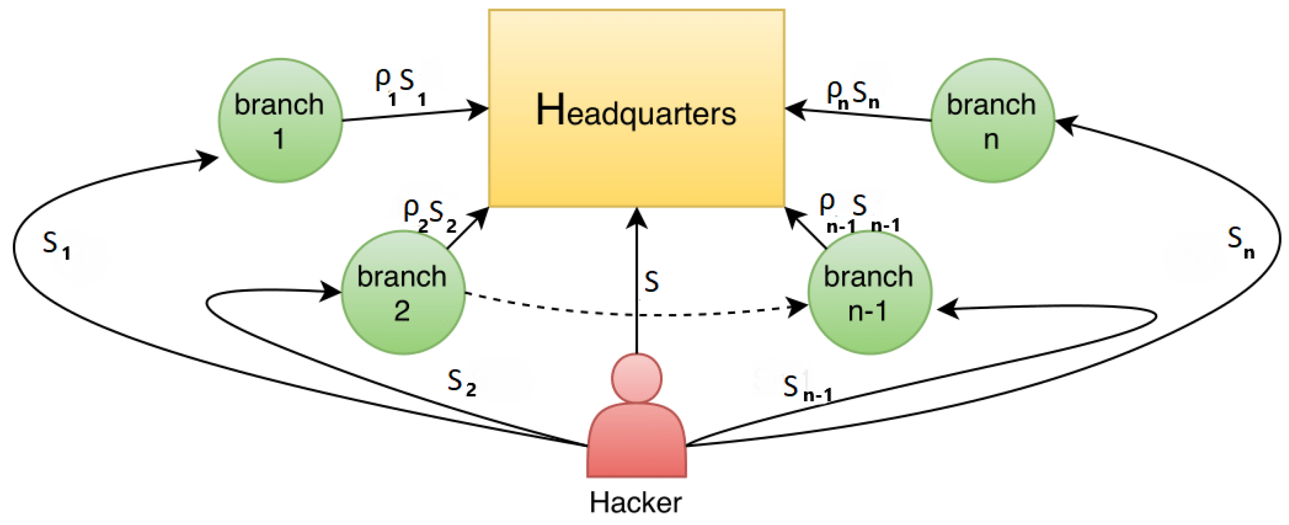
In Section 3, we describe the scenario with a single-site firm and its insurance liability options. In this section, we move to a multi-branch firm, where the vulnerability of the branches influences that of the headquarters. We modify the breach probability function for the headquarters, considering a unilateral influence as in Khalili et al. (2017), from the branches to the headquarters but not vice versa. We set the framework for the multi-branch case, reporting the overall security expenses for the headquarters and the branches under the three liability cases described in Section 3. We consider the scenario of Figure 1, where a company has n branches, and the hacker may attack any subset of these sites’ information systems. Each branch exhibits a (generally different) vulnerability level and decides its own security investments, as does the headquarters. We use the symbol z for the security investments of the headquarters, while represents the investments of the ith branch. Similarly, we use v and for the no-investment vulnerability of the headquarters and the ith branch, respectively, and P and for the insurance premiums.
- direct breach, due to a direct attack on the headquarters; and
- indirect breach, due to breaches taking place on branches.
For the ith branch, as for the headquarters, the security probability function follows the Gordon–Loeb model:
We can now determine the overall security expense for the generic ith branch by summing the investment and the insurance premium for the three liability cases, as described in Section 3, i.e., full liability, limited liability, and deductibles.
For the case of full liability, the expense born by the ith branch is
If the insurance policy includes an upper limit to the liability of the ith branch, the overall expense is instead
where is the probability of an attack taking place on the ith branch.
If the insurance policy also includes a deductible , the overall expected expense for the ith branch is
We can now turn to the headquarters. As hinted before, the attacks on the branches may further endanger the security of the headquarters, so that we must consider indirect breaches as well. We define first the probability of a direct attack being successful, again through the Gordon–Loeb model:
As to the indirect attack, we model the impact of an attack taking place on the ith branch through the probability of an indirect attack propagation. If we assume that the headquarters may suffer from either a direct attack or an indirect one through any of its branches, and direct attacks and indirect attacks take place independently of one another, the overall probability of the headquarters being breached is
Similarly to what is done for the branches, we can finally compute the security expense for the headquarters, again for the three coverage cases.
For the full liability case, we have
If the insurance policy includes a maximum liability equal to T, the overall security expense becomes
If a deductible F is also factored in, we have
5. Optimal Investment for the Headquarters
After describing the overall expenses in the case of a multi-branch firm in Section 4, we focus now on the headquarters and obtain the optimal investment in the headquarters’ security, considering a unilateral influence from the branches to the headquarters but not vice versa, as in Khalili et al. (2017). We consider the three liability cases described in Section 3.
5.1. Full Liability
We consider first the branches and then the headquarters.
To find the optimal investment for the ith branch, we can exploit the result reported in Mazzoccoli and Naldi (2019):
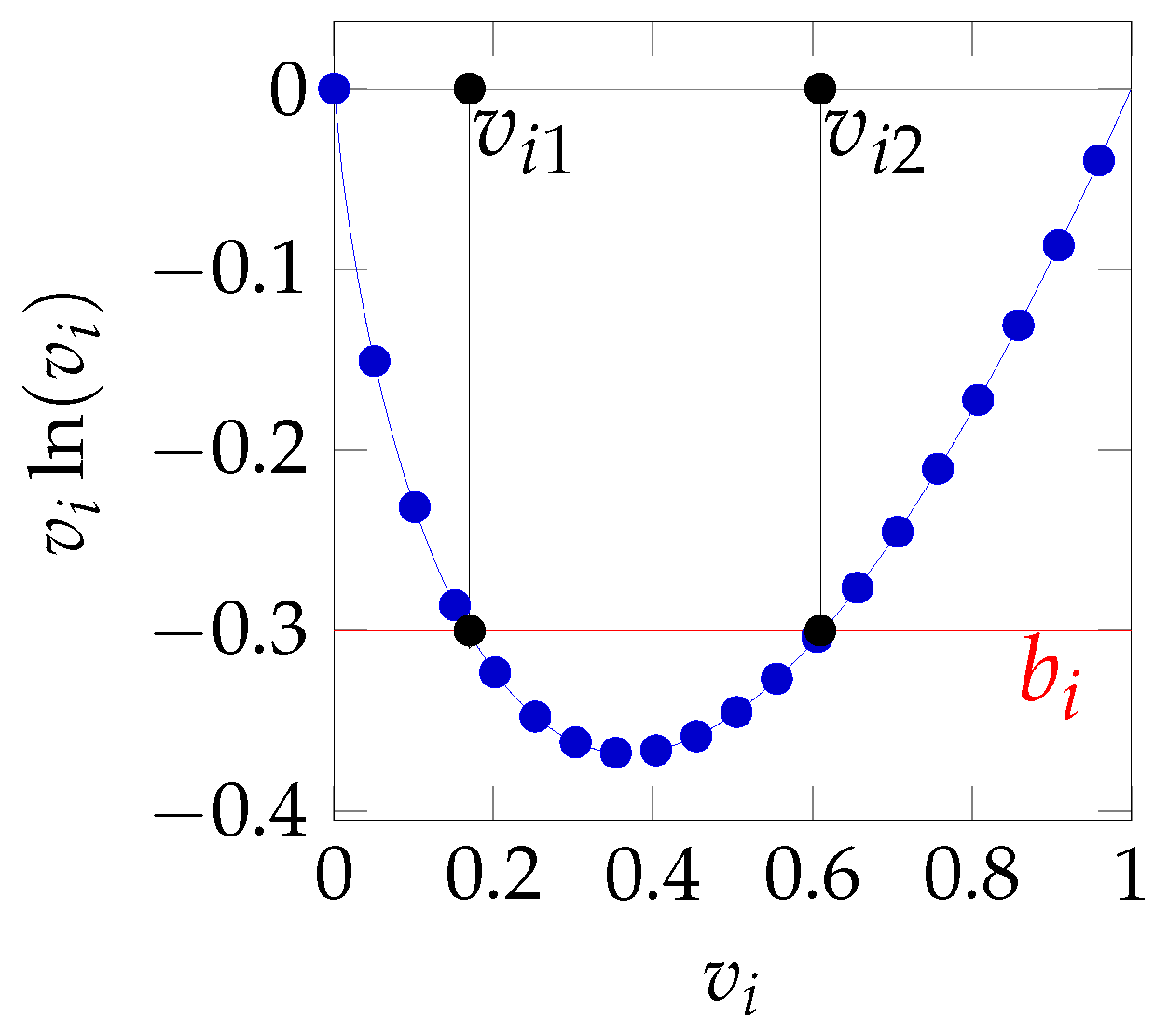
We need to check whether this solution is a valid one, i.e., , which is equivalent to the following condition:
The function on the left hand side of this inequality is shown in Figure 2.
If we set the threshold
we see that the equation is solved for two values and . The inequality is satisfied if the vulnerability lies between those two values (). We observe then a region of intermediate vulnerability values for which the solution obtained from Equation (13) is a valid (positive) investment. It pays to invest in security as long as the intrinsic vulnerability (i.e., in the absence of investments) is neither too high (above ) nor too low (below ), as shown by Mazzoccoli and Naldi (2019).
We can now turn to the headquarters. In Appendix A, we obtain the optimal investment for the headquarters
As we can see, the overall investment for the headquarters also depends on the security characteristics of the branches, in particular through their intrinsic vulnerability and the investments in security made by the branches themselves. We wish to highlight that contribution by defining the coefficient of branch influence
It can be noted that, if the headquarters were not dependent on the security of the branches, we would have . Since that coefficient lies in the (0, 1] range and decreases when the dependence coefficients grow, values closer to 0 mark a larger dependence on the security of the branches.
We can now check whether the conditions for the validity of the investment apply:
- is positive.
- is a point of minimum for .
We report the detailed analysis in Appendix B. We see that the following conditions may lead not to invest in security:
- Low insurance premium
- Low potential loss
- Low probability of attack
- Low discount rate offered on the premium
- Low effectiveness of security investments
- Too high or too low vulnerability of the branches
By investing the amount , the headquarters minimize their overall expenditure, which is finally
For the purpose of assessing the behavior of this expense, we adopt hereafter the parameters listed in Table 2 and Table 3 for the headquarters and the branches, respectively. The values in these tables are taken from Young et al. (2016) and Mazzoccoli and Naldi (2019). For the sake of simplicity, we consider all the branches to be equal. We see now how the investments made by the branches and their intrinsic vulnerability impact on the optimal investment the headquarters are called to make.
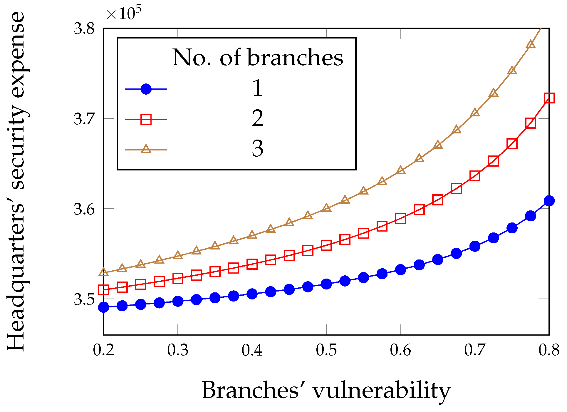
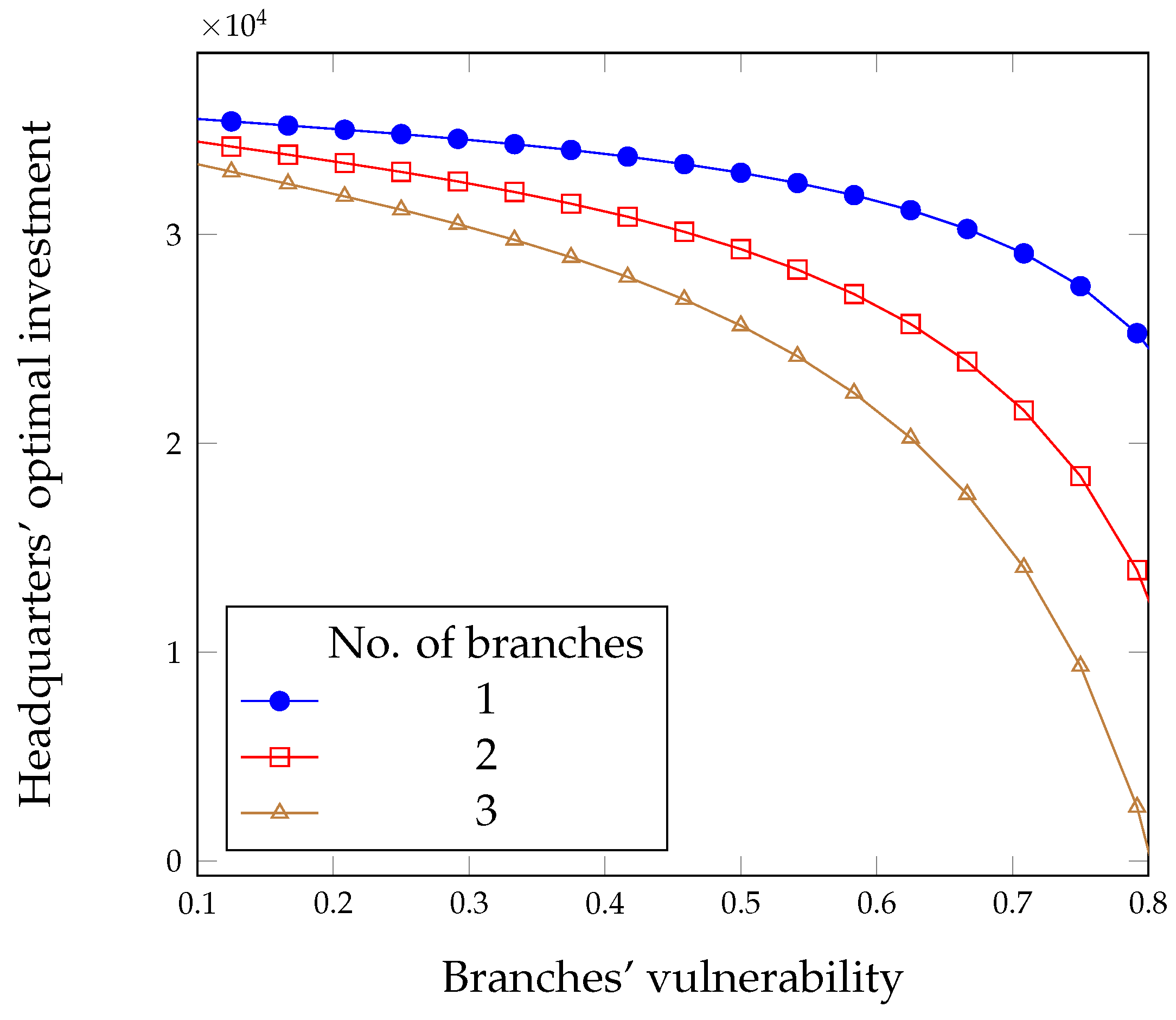
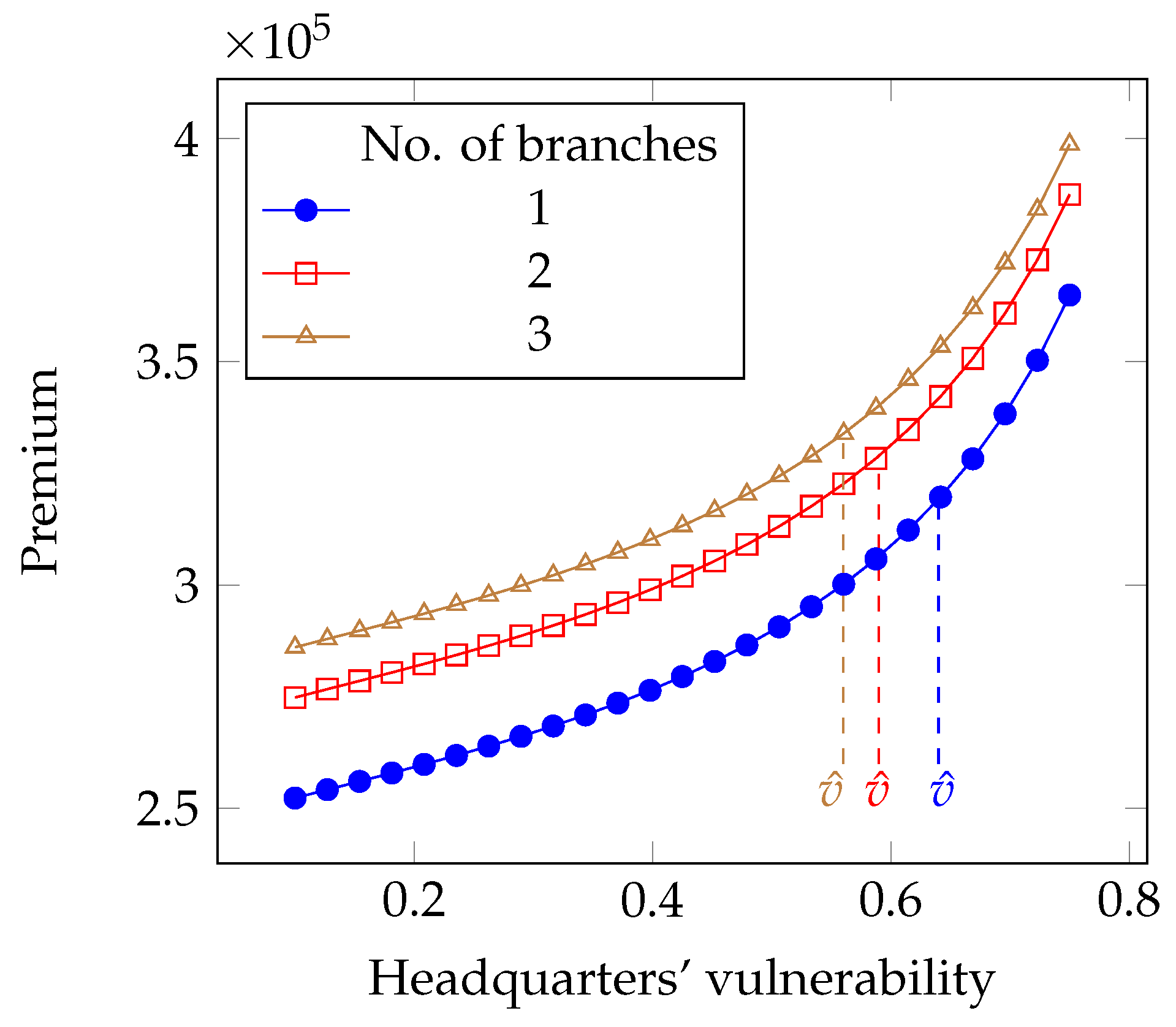
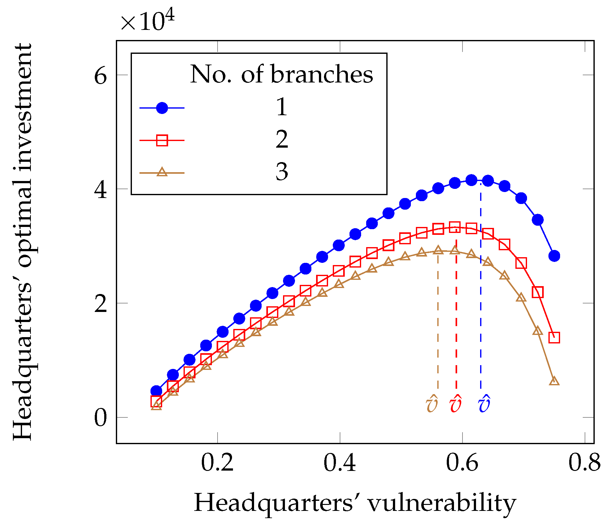
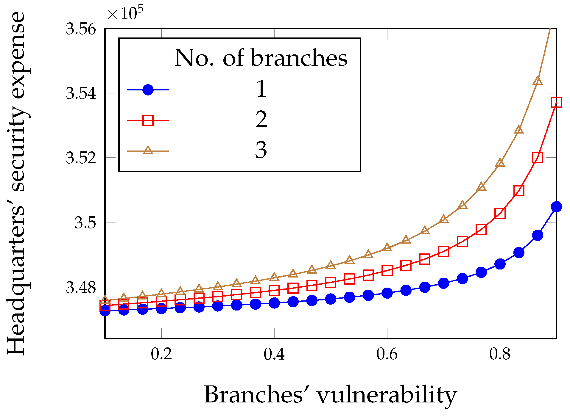
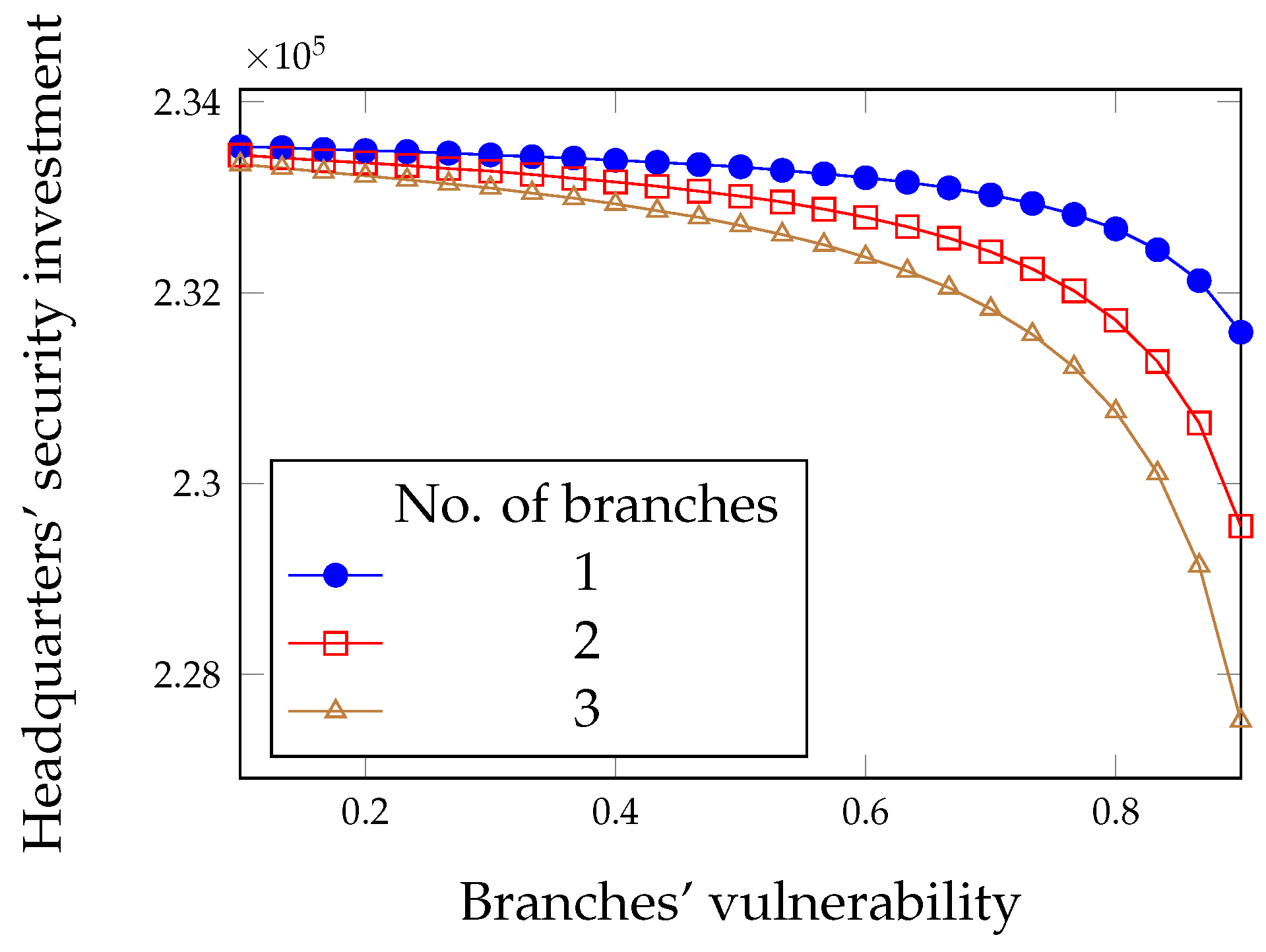
Since we wish to investigate the influence of branches on the headquarters, we start by seeing how the vulnerability of the branches influences the headquarters’ expense. We see in Figure 3 that the vulnerability of the branches impacts negatively, since the headquarters’ overall expense increases when the branches get more vulnerable. However, there is a counter-intuitive behavior of the other component of security expense, i.e., the investment: we see in Figure 4 that the headquarters are called to invest less as the branches get more vulnerable.
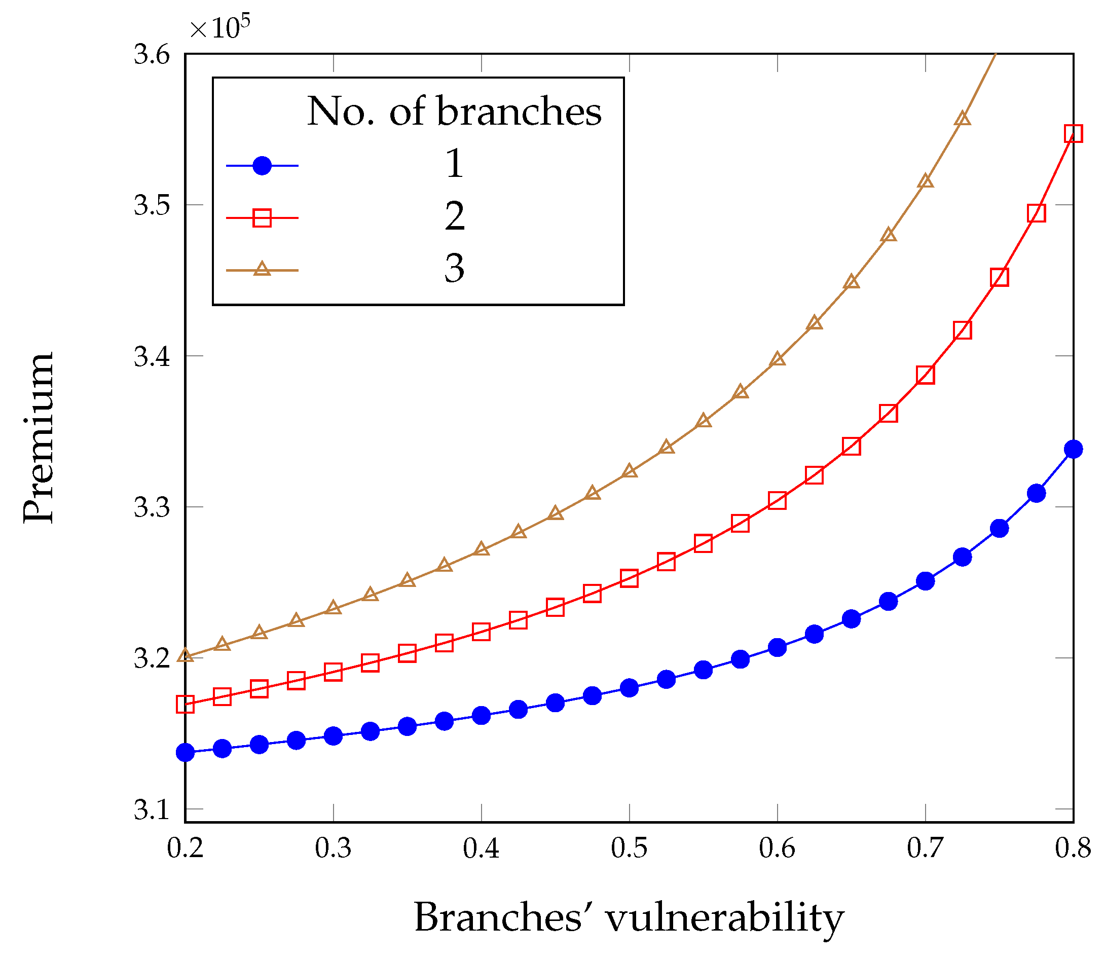
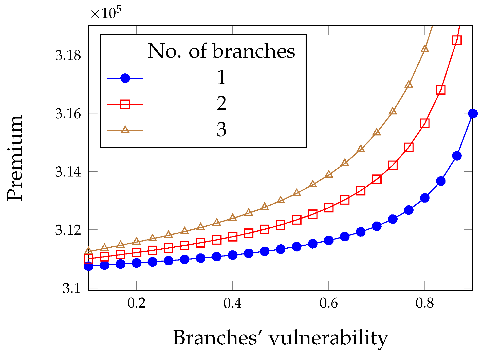
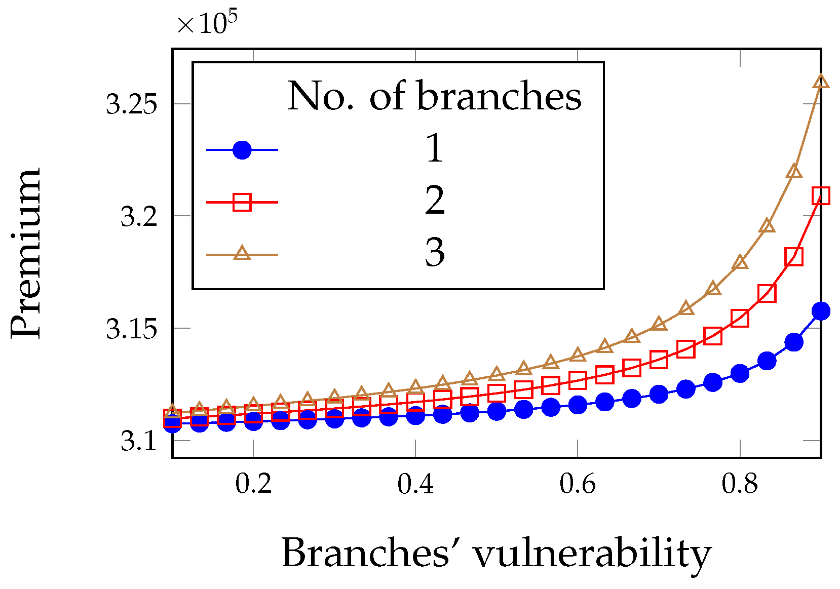
Hence, although the overall effect is negative, the impact of the branches behavior on the two components of security expense is different. In particular, the premium represents by far (roughly by a factor of ten) the major component, and its trend is reflected in the overall expense (see Figure 5).
We can now investigate the impact of the intrinsic vulnerability v of the headquarters. To provide concrete figures, we assume that the basic premium is set as a fraction of the expected loss, i.e., . This premium setting mechanism follows the well known expected value principle, as described by Goovaerts et al. (2001), in Section 5.3. It is also known as flat-rate pricing, which is reported to be used by 50% of insurance companies in a recent survey by Romanosky et al. (2017). As expected, the insurance premium grows non-linearly with the vulnerability (see Figure 6).
Instead, the other component of the overall security expenses, i.e., the investment, is not a monotone function of the vulnerability. In Figure 7, we can observe that the optimal investment in security grows up till the vulnerability reaches the value and then decreases. When the vulnerability is either low or high, it is probably not worth investing in security, but instead relying on the total protection afforded by an insurance policy. Investing is instead heavily required when the vulnerability lies in the intermediate range. The vulnerability value marking the center of that intermediate region can be identified by looking for the maximum investment condition:
5.2. Limited Liability
We consider the case where the insurance company does not cover all the losses. The limit coverages for the headquarters and the ith branch are, respectively, T and .
In this case, after recalling Equations (2) and (5), the overall expense for the ith branch is the following:
Using similar arguments as in the previous subsection, we need to check whether the optimal investment is valid, i.e., . Thus, we find that this condition is satisfied if
Introducing the threshold
we see that equation identifies two values and , delimiting a region of intermediate vulnerability values, , for which the investment defined by Equation (21) is a valid one.
Now, we turn to the headquarters. In Appendix C, we derive the optimal investment for the headquarters
where we introduce the coefficient of branch influence in limited liability regime
Now, we check Conditions (a) and (b) as in Section 5.1 for the validity of the optimal investment. We report the detailed analysis in Appendix D. We prove that the optimal investment actually leads to minimizing the overall security expenses and that it pays to invest when the vulnerability lies in an intermediate region.
Comparing the conditions for investing represented by Equations (A6) and (A14), we can observe that the range of vulnerability values for which the headquarters find it convenient to invest in security increases when we have limited liability.
If the combination of , , T, t, r, and is such that , there is no vulnerability value that allows obtaining a convenient investment. The no-investment condition takes place when
Thus, it does not pay to invest in security when the premium rate lies below the threshold .
By investing the amount , the headquarters minimize their overall expenditure, which is finally
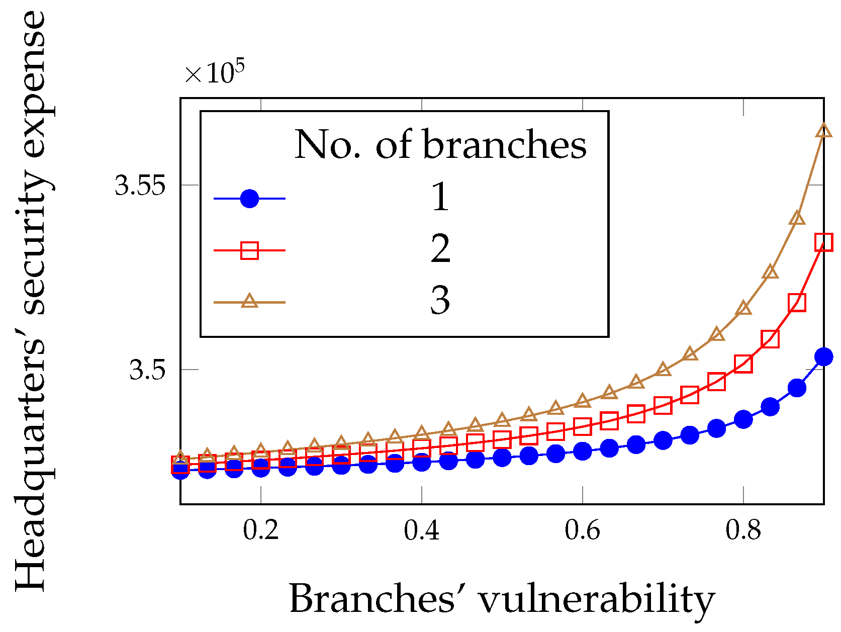
In addition, in this case, we see in Figure 8 that more vulnerable branches compel the headquarters to spend a bit more in security. However, the investment in security and the insurance premium exhibit now the same order of magnitude, as can be seen in Figure 9 and Figure 10. When the vulnerability of the branches grows, security investments become the smaller portion of the overall expense since insurance becomes the preferred means of achieving protection.
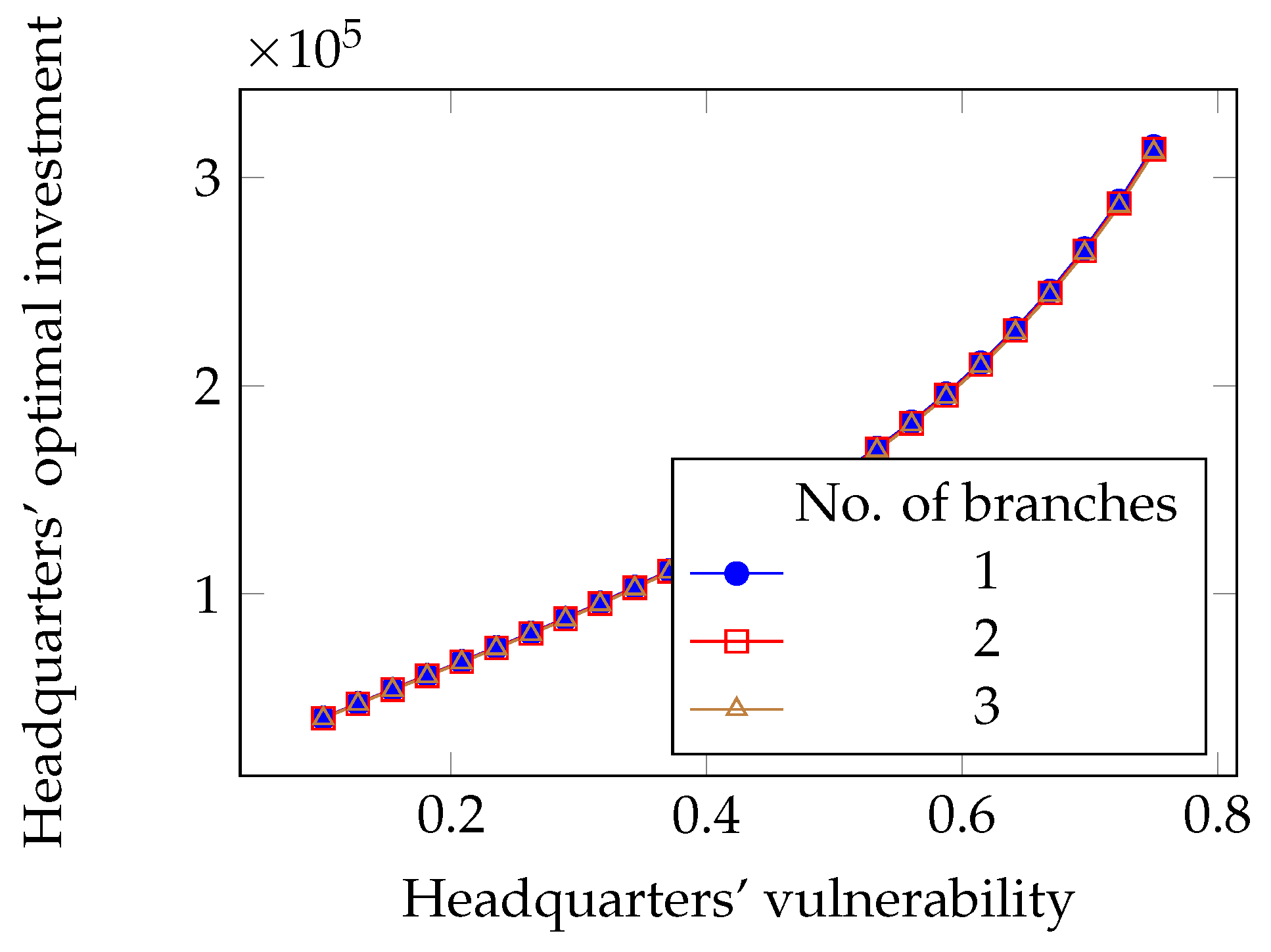
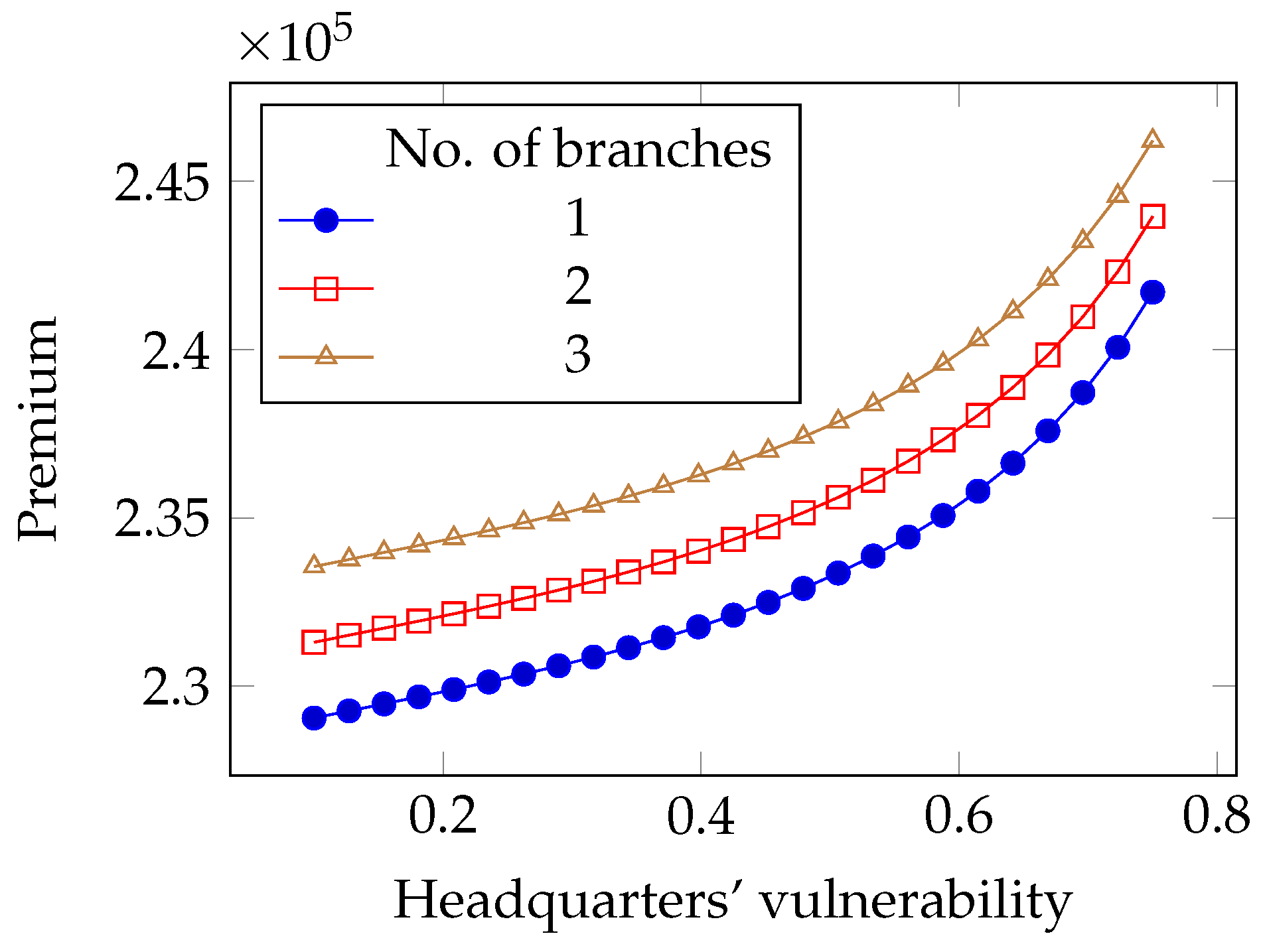
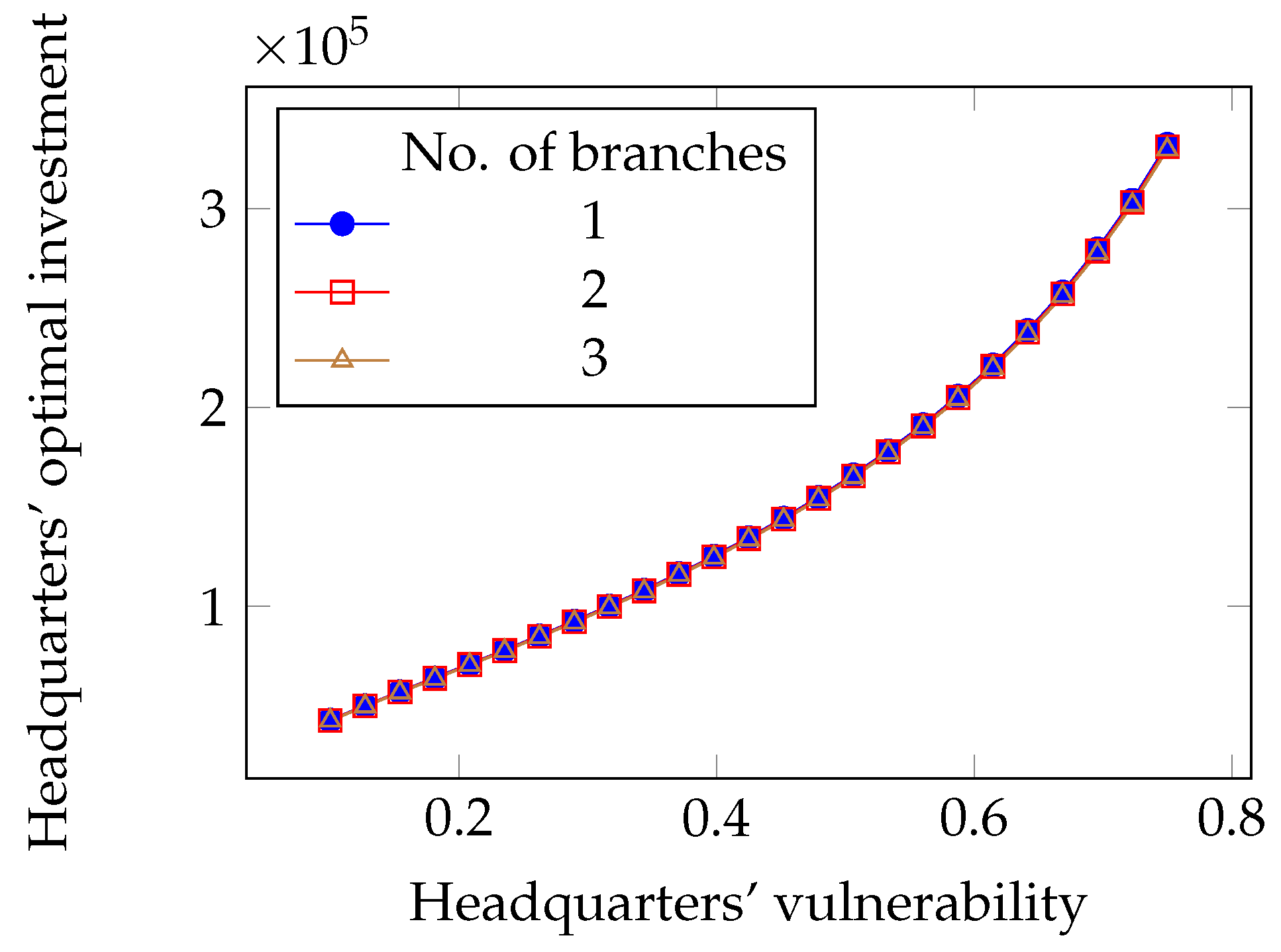
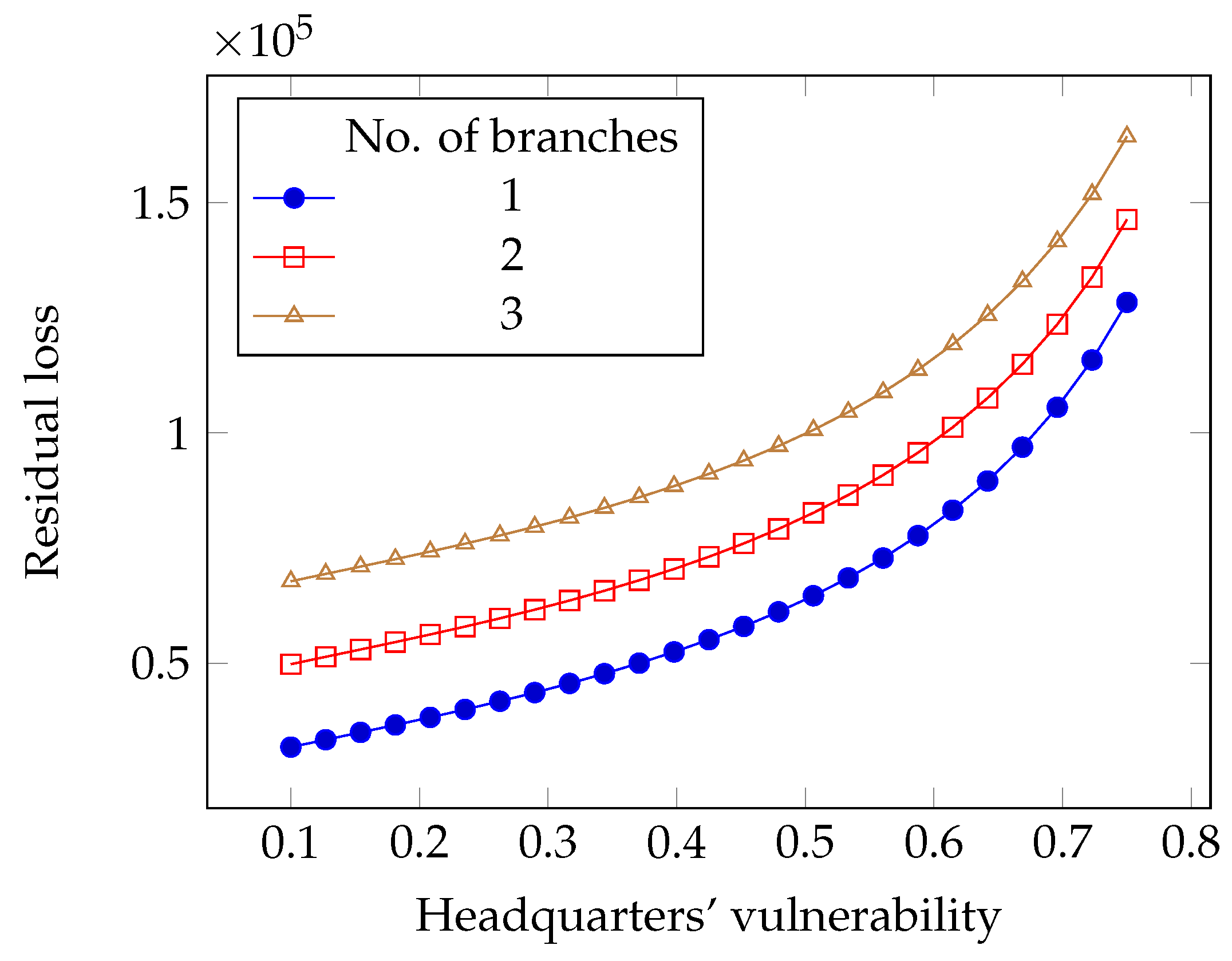
Finally, contrary to what happens in the full liability case, both components of security expense for the headquarters grow with its intrinsic vulnerability, as can be seen in Figure 11 and Figure 12. In Figure 11, it can be seen that the number of branches has practically no impact on the optimal investment: the effect was magnified in plotting Figure 10 but is actually very limited. Instead, the impact of the number of branches on the insurance premium is significant.
5.3. Limited Liability with Deductibles
Now, we consider the case where insurance companies provide limited coverage (with limit coverage, respectively, for the ith branch and T for the headquarters) but impose deductibles as well, described by and F for the ith branch and the headquarters, respectively.
For simplicity of notation, we define by and the following quantities for the ith branch and the headquarters, respectively,
The expenses for the ith branch and the headquarters are, respectively,
The optimal investment for the ith branch is then
Similarly to what we is done for the alternative liability cases, we wish to see when it pays to invest in security, i.e., , which is tantamount to the following condition:
Again, we define the threshold
so that, again, we find two values and through solving the equation . Again, the inequality is satisfied if the . We have therefore a region of vulnerability values that makes the solution obtained from Equation (32) a valid investment.
Since the second-order derivative is positive, we can be sure that the expense is at its minimum:
We see in Appendix F that it does not pay to invest in security if the basic premium is
By investing the amount , the headquarters minimize their overall expenditure, which is finally
6. Robustness of Security Investment Decisions
As derived in Section 5, the optimal investment depends on several variables. We know some of them exactly: we know the premium , the maximum liability T, and the deductibles F. However, some other variables influencing the optimal investment in security are the result of estimates: we must estimate the potential damage , the probability of attack t, the vulnerability v, and the investment effectiveness coefficient . This applies not just to the headquarters but to all branches as well. In Mazzoccoli and Naldi (2019), the authors paid attention to the vulnerability v and the investment effectiveness as potential sources on uncertainty in the estimates. Here, we focus instead on the coefficient of branch dependence and branch vulnerability . In this section, we assess that impact by determining how sensitive the optimal investment is to inaccuracies in and . For that purpose, we employ the quasi-elasticity function. We recall that the general concept of elasticity provides a means for estimating the response of one variable to changes in some other variable (e.g., the price elasticity of demand tells us how the demand varies when the price changes), as defined, e.g., in Chapter 17 of Arnold (2008) and Chapter 6 of Krugman and Wells (2009). A review of its application in economics is reported in Nievergelt (1983). Examples of its application outside economics are shown in Guijarro et al. (2019); Naldi et al. (2019). Quasi-elasticity has to be used in the place of elasticity when the independent variable lies naturally within the [0, 1] range, so that its absolute value can also be expressed as a percentage. Quasi-elasticity is defined as the ratio of the relative variations of the response variable to the variations of the independent variable. The quasi-elasticity function measures therefore the percentage change in the response variable when the independent variable changes by 0.01. In our case, we consider first the optimal investment (for the time being, we do not specify whether it is , or ) as the response variable and the coefficient of branch dependence and then the branch vulnerability as the independent variable. In particular, we define the quasi-elasticity of the optimal investment with respect to the coefficient ( or ) as follows
In the hereafter reported examples, we adopt the parameters reported in Table 2 and Table 3, excluding the parameter under consideration ( or , respectively).
6.1. Quasi-Elasticity under Full Liability
For the full liability case, the quasi-elasticity with respect to is
and that with respect to is
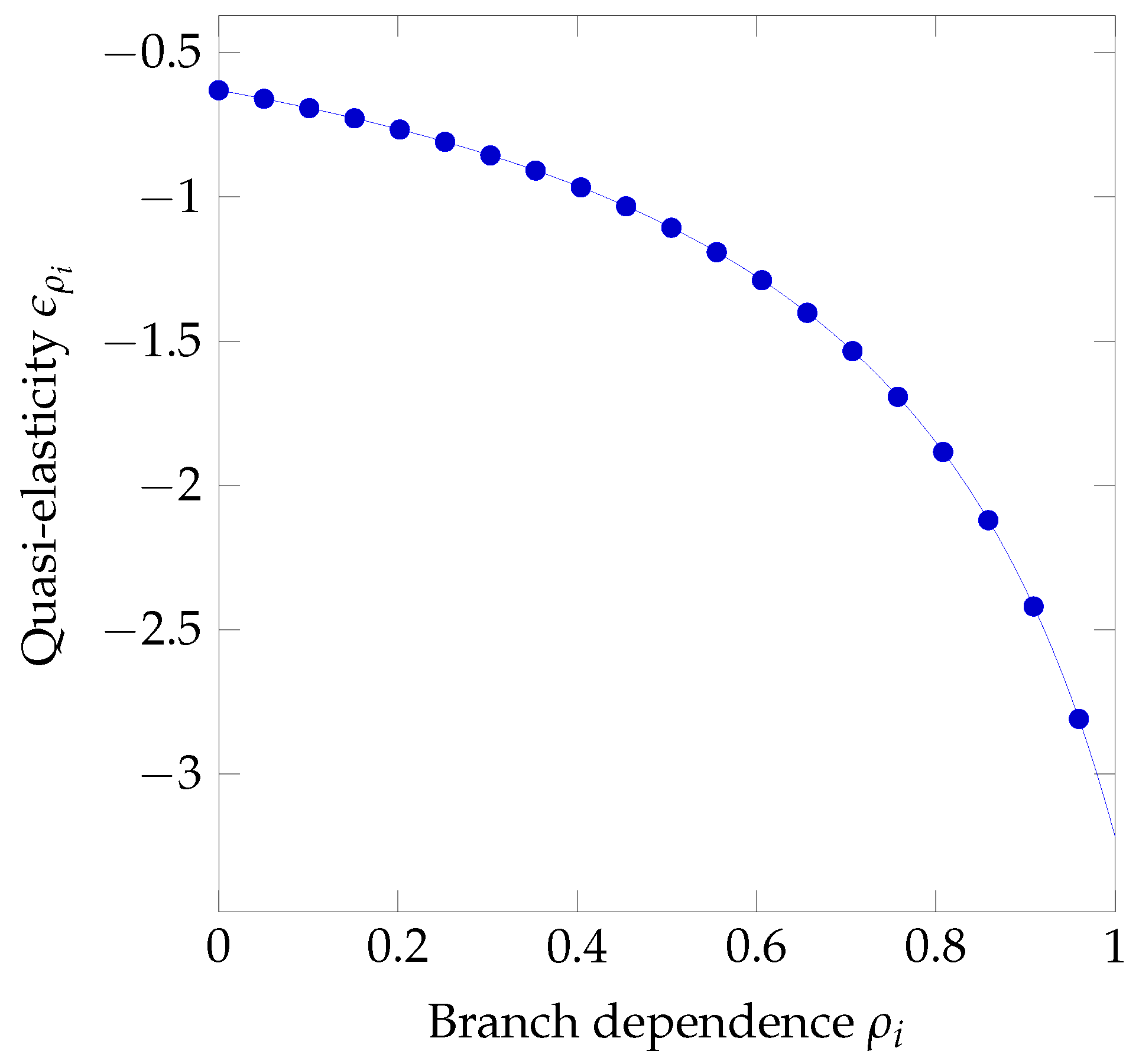
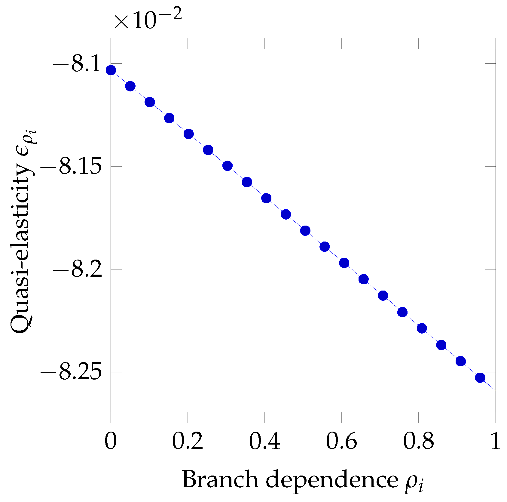
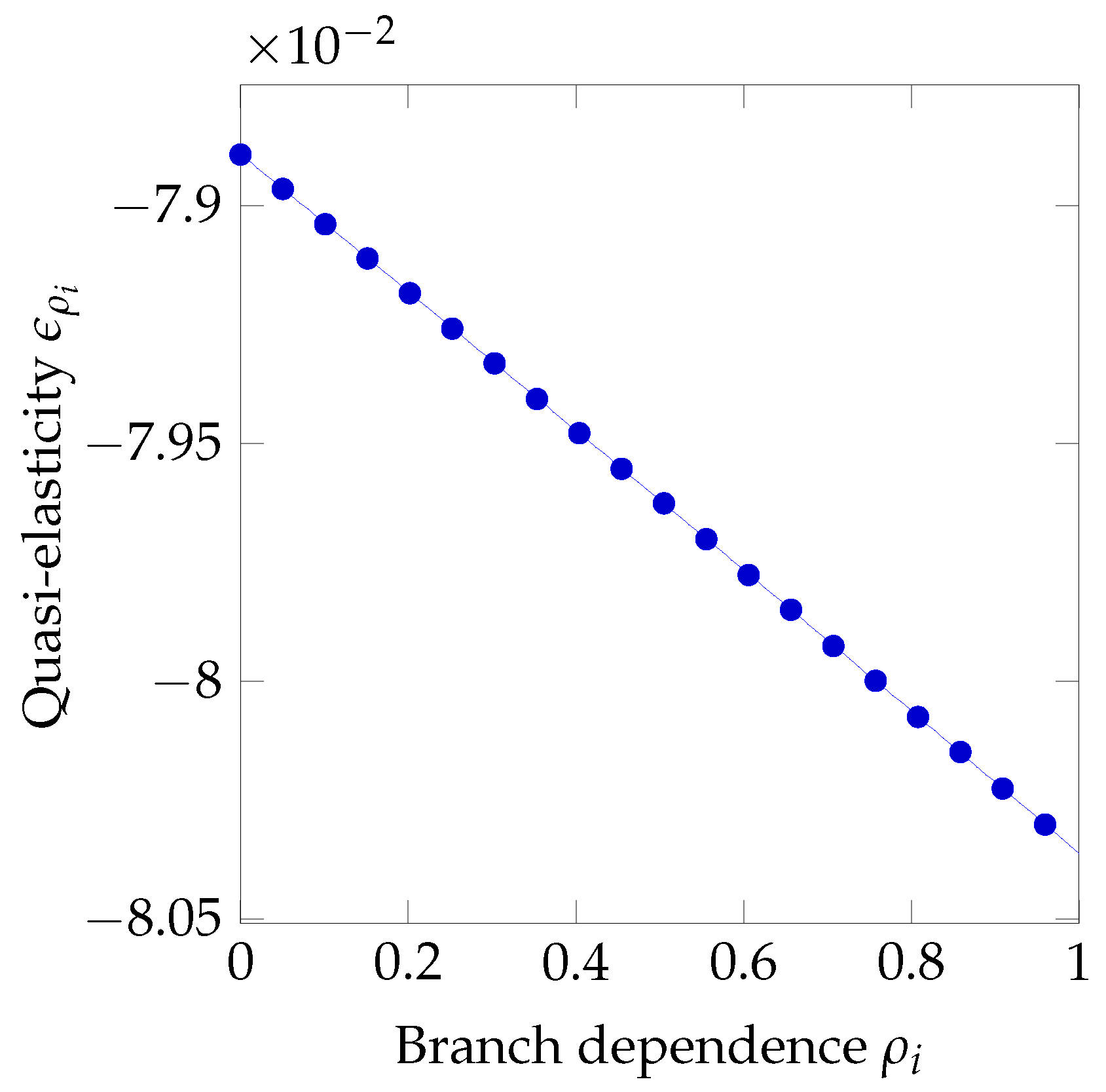
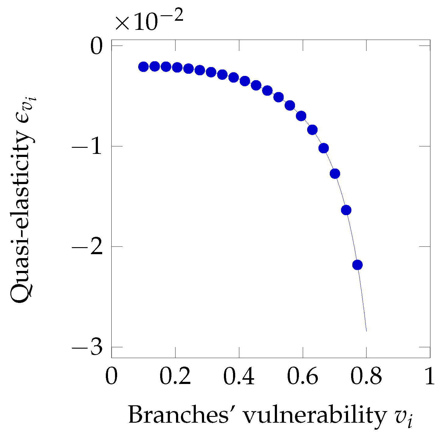
The quasi-elasticity is always negative for both cases, which is somewhat counter-intuitive: if the influence of branches or their vulnerability increase, the headquarters are led to invest less in security. When we come to the extent of the impact (i.e., the value of the quasi-elasticity rather than just its sign), in the case of the dependence from branches , we can note two regions in Figure 19. The behavior is first inelastic (), when the dependence is low (roughly ). When the security of the headquarters is strongly influenced by that of the branches, the quasi-elasticity turns heavily negative, with the investment in security reducing even by 3% when the branch dependence changes, e.g., from 0.9 to 0.91. Misestimating the dependence coefficient from branches may then become dangerous when the dependence is high: overestimating it would lead to reducing the investment (hence, suffering heavier losses).
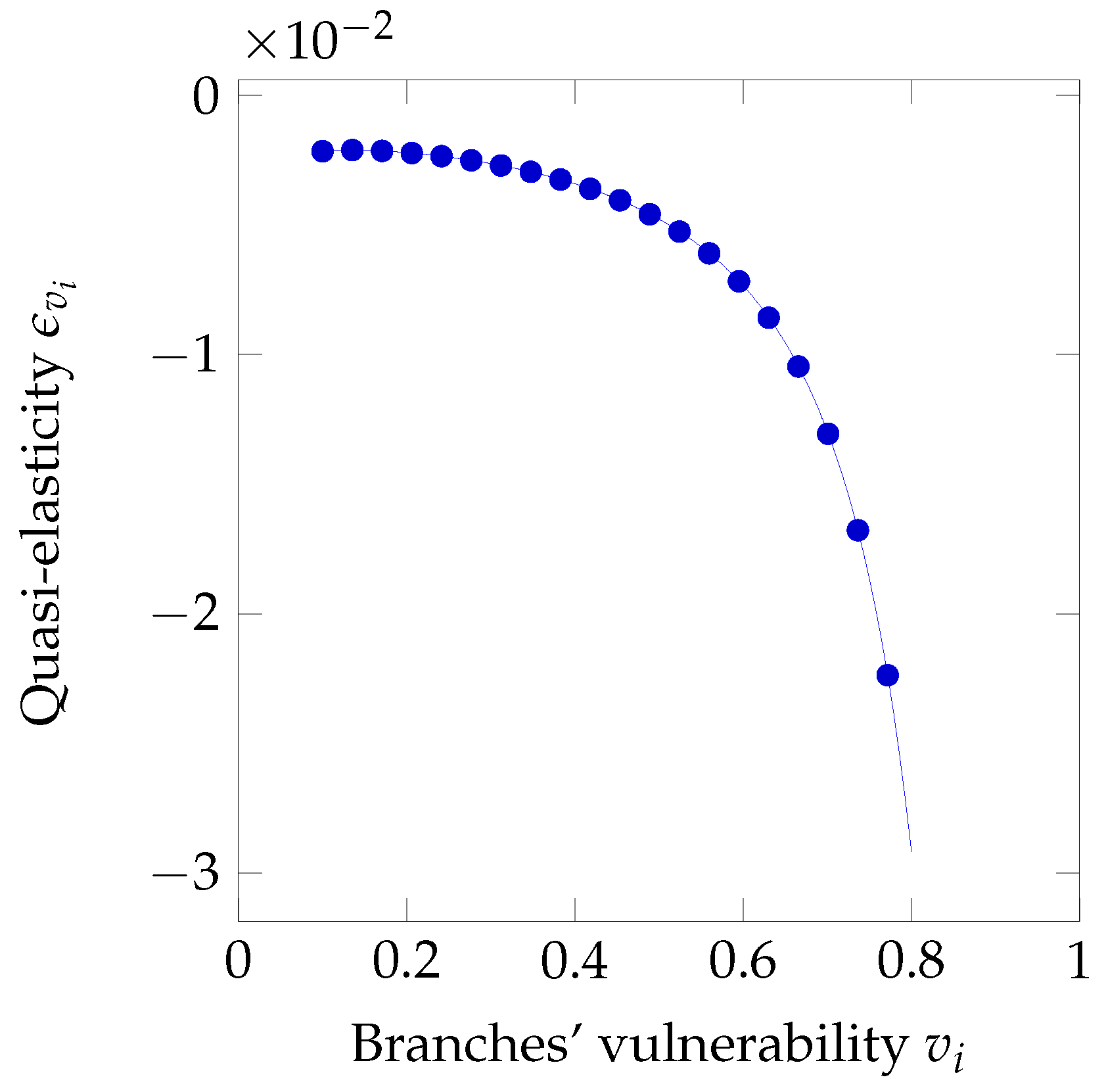
We observe a similar behavior for the quasi-elasticity with respect the vulnerability of branches in Figure 20. The vulnerability value marking the passage from the inelastic region to the elastic one is .
6.2. Quasi-Elasticity under Limited Liability
In the case of limited liability, we find similarly the quasi-elasticity expressions reported hereafter:
6.3. Quasi-Elasticity under Limited Liability with Deductibles
Finally, we derive the quasi-elasticity when we also introduce deductibles:
7. Conclusions
The investigation into the optimal strategies when both insurance and security investments are used to reduce the security-related losses in a multi-branch company allows us to understand the actual impact of vulnerabilities in the branches on the headquarters’ behavior. The vulnerability of branches may bear a significant influence on the overall expenses in security for the headquarters. As the vulnerability of the branches increases, the headquarters are led to invest less in security (which may appear somewhat counter-intuitive) but to rely more on insurance. In particular, if the vulnerability is very low or gets very high, it does not pay to invest in security. However, the relative size of effects is quite different: the impact of branches’ vulnerability is much higher on the insurance premium than on investments.
In addition, the mix of security countermeasures suggested by the analysis is quite imbalanced, with insurance being by far the largest component in the overall expense.
However, we must consider that the actual amount of expenses suggested by the strategies relies on the accuracy of the input variables to be estimated, in particular the vulnerability of the branches themselves and the correlation between breaches taking place on the branches and security incidents in the headquarters. Actually, we can conclude that the impact of uncertainty in the assessment of the degree of influence that branches have on headquarters is not to be overemphasized, since an amplification effect is present just for the smaller values of vulnerability (i.e., when the investment is relatively small). In addition, the amount of investment is quite insensitive to the precise assessment of the branches’ vulnerability for a large range of values, unless when the vulnerability gets very high, in which case a sudden amplification of the impact takes place. Since no investment is recommended in the regions of very low and very high vulnerability, we can conclude that the impact of the uncertainty on correlation and vulnerability is not significant in most cases.
We add some final notes as possible hints for future work.
Our study was conducted under the hypothesis that investment decisions follow a decentralized approach, where the branches decide for themselves. This is a sensible approach, since the branches may know better their actual security status than what the headquarters could, but it may not be the optimal choice. A comparison with a centralized approach, where the headquarters set the optimal level of investments for all the branches as well, with the aim of optimizing the overall expenses, should be investigated. In addition, we considered one of the Gordon–Loeb breach probability functions. Although this is an established choice, well rooted in the literature, different functions could be explored to reflect the changing impact of security investments on the actual security level. Finally, different interdependence models could be considered, e.g., by removing the unilateral effect (from the branches to the headquarters, but not vice versa) considered in this paper.
Author Contributions
Conceptualization, A.M. and M.N.; methodology, A.M. and M.N.; software, A.M.; validation, A.M. and M.N.; formal analysis, A.M. and M.N.; investigation, A.M. and M.N.; resources, M.N.; data curation, A.M.; writing—original draft preparation, A.M. and M.N.; and writing—review and editing, A.M. and M.N. All authors have read and agreed to the published version of the manuscript.
Funding
This research received no external funding.
Conflicts of Interest
The authors declare no conflict of interest.
Appendix A. Optimal Investment of Headquarters under Full Liability
After recalling Equations (8) and (9), and plugging in the optimal investment for the branches of Equation (13), the overall expense for the headquarters is
By zeroing the derivative of the expense with respect to the investment z
we obtain the optimal investment for the headquarters
Appendix B. Validity Conditions for the Investments of the Headquarters under Full Liability
As stated in the main body of the paper, we have to check the following two conditions, which guarantee that the decision to invest in security is correct:
- (a)
- is positive.
- (b)
- is a point of minimum for .
We first check the conditions for the minimization of security expenses. Since the second-order derivative is
and a product of positive quantities, it is positive: is then a point of minimum (satisfying Condition (b)).
Now we have to check Condition (a) and see when the optimum investment is positive (which is equivalent to say that it pays to invest in security).
From Equation (18), recalling that , the investment is positive if
As can be seen in Figure 2 (by using v in the place of ), after re-defining the threshold
the equation , identifies two values and , so that the inequality is satisfied if . The solution obtained from Equation (18) is a valid (positive) investment if the vulnerability lies in that region. If we set the reference value , i.e., equal to b in the special case when there is no dependence on the branches’ security (i.e., ), we see that , so that the range of vulnerability values for which it pays to invest in security shrinks when the security of the branches impacts on that of the headquarters (see Figure 2).
If the combination of values , , t, r, and is such that , there is no vulnerability value that allows to obtain an optimal investment: the no-investment condition takes place when the basic premium is such that
According to the definition of the threshold b in Equation (A6), one or more of the following conditions could have the company decide not to invest in security:
- Low insurance premium
- Low potential loss
- Low probability of attack
- Low discount rate offered on the premium
- Low effectiveness of security investments
- Too high or too low vulnerability of the branches
The result obtained in Equation (A7) confirms what was found by Gordon and Loeb (2002) for the case of security investment only (and for a single firm). In this new context as well, where an insurance premium is paid and the headquarters security depends on the branches, it may not pay to invest in security.
Appendix C. Optimal Investment of Headquarters under Limited Liability
Recalling Equations (8) and (11), and plugging in the optimal investment for branches computed in Equation (21), the overall security expense for headquarters is
Thus, zeroing the derivative of the expense in Equation (A8) with respect to the investment z
we obtain the optimal investment for the headquarters
where is the coefficient of branch influence in limited liability regime, defined as follows
It can be observed that has properties similar to , described in Equation (17).
Appendix D. Validity Conditions for the Investments of the Headquarters under Limited Liability
Now, we check Conditions (a) and (b) as in Section 5.1 for the validity of the optimal investment. In addition, in this case, we start by checking the condition for the minimization of the security expenses. We can state that Condition (b) is satisfied since the second-order derivative
is positive, as it is a product of positive quantities.
Now, we have to check Condition (a), i.e., we want to analyze when the optimum investment is positive.
Recalling Equation (A10), we have if
As in the full liability case (see Figure 2), we can define the threshold
We see that the equation is solved by two values and so that the inequality of Condition (a) is satisfied if .
Appendix E. Optimal Investment of Headquarters under Deductibles
Since the expense for the headquarters is
we can define the following quantity
which represents how much the headquarters are influenced by their branches.
We can obtain the optimal investment by zeroing the derivative of Equation (A15), whose solution is
Appendix F. Validity Conditions for the Investments of the Headquarters under Deductibles
Since the second-order derivative is positive, we can be sure that the expense is at its minimum:
Finally, we see when the optimum investment is indeed positive:
After redefining the threshold
we can see that the equation is solved by two values and so that the inequality is satisfied if . The no-investment condition takes place when
i.e., if the basic premium is
References
- Arnold, Roger. 2008. Economics, 8th ed. Mason: Thomson South-Western. [Google Scholar]
- Bandyopadhyay, Tridib, Vijay S. Mookerjee, and Ram C. Rao. 2009. Why IT managers don’t go for cyber-insurance products. Communications of the ACM 52: 68–73. [Google Scholar] [CrossRef] [Green Version]
- Bolot, Jean, and Marc Lelarge. 2009. Cyber insurance as an incentive for internet security. In Managing Information Risk and the Economics of Security. Berlin: Springer, pp. 269–90. [Google Scholar]
- Bryce, Robert. 2001. Hack Insurer Adds Microsoft Surcharge. Available online: https://www.zdnet.com/article/hack-insurer-adds-microsoft-surcharge/ (accessed on 16 December 2020).
- Eling, Martin, and Jan Wirfs. 2019. What are the actual costs of cyber risk events? European Journal of Operational Research 272: 1109–19. [Google Scholar] [CrossRef]
- Goovaerts, Marc, Rob Kaas, Jan Dhaene, and Michel Denuit. 2001. Modern Actuarial Risk Theory. Berlin: Springer. [Google Scholar]
- Gordon, Lawrence A., and Martin P. Loeb. 2002. The economics of information security investment. ACM Transactions on Information and System Security 5: 438–57. [Google Scholar] [CrossRef]
- Gordon, Lawrence A., Martin P. Loeb, and Tashfeen Sohail. 2003. A framework for using insurance for cyber-risk management. Communications of the ACM 46: 81–85. [Google Scholar] [CrossRef]
- Gordon, Lawrence A., Martin P. Loeb, and Lei Zhou. 2016. Investing in Cybersecurity: Insights from the Gordon-Loeb Model. Journal of Information Security 7: 49. [Google Scholar] [CrossRef] [Green Version]
- Guijarro, Luis, Jose R. Vidal, Vicent Pla, and Maurizio Naldi. 2019. Economic analysis of a multi-sided platform for sensor-based services in the internet of things. Sensors 19: 373. [Google Scholar] [CrossRef] [Green Version]
- Guo, Hong, Hsing Kenneth Cheng, and Ken Kelley. 2016. Impact of network structure on malware propagation: A growth curve perspective. Journal of Management Information Systems 33: 296–325. [Google Scholar] [CrossRef]
- Kesan, Jay P., Rupterto P. Majuca, and William J. Yurcik. 2004. The Economic Case for Cyberinsurance. Technical Report 2. Champaign: University of Illinois College of Law. [Google Scholar]
- Khalili, Mohammad Mahdi, Parinaz Naghizadeh, and Mingyan Liu. 2017. Embracing risk dependency in designing cyber-insurance contracts. Paper presented at 2017 55th Annual Allerton Conference on Communication, Control, and Computing (Allerton), Monticello, IL, USA, October 3–6; pp. 926–33. [Google Scholar]
- Khalili, Mohammad Mahdi, Parinaz Naghizadeh, and Mingyan Liu. 2018. Designing cyber insurance policies: The role of pre-screening and security interdependence. IEEE Transactions on Information Forensics and Security 13: 2226–39. [Google Scholar] [CrossRef]
- Kröger, Wolfgang. 2008. Critical infrastructures at risk: A need for a new conceptual approach and extended analytical tools. Reliability Engineering & System Safety 93: 1781–87. [Google Scholar]
- Krugman, Paul, and Robin Wells. 2009. The Rational Consumer. New York: Worth Publishers. [Google Scholar]
- Kshetri, Nir. 2020. The evolution of cyber-insurance industry and market: An institutional analysis. Telecommunications Policy 44: 102007. [Google Scholar] [CrossRef]
- Levitin, Gregory, Liudong Xing, and Yuanshun Dai. 2018. Co-residence based data vulnerability vs. security in cloud computing system with random server assignment. European Journal of Operational Research 267: 676–86. [Google Scholar] [CrossRef]
- Maglaras, Leandros A., Ki Hyung Kim, Helge Janicke, Mohamed Amine Ferrag, Stylianos Rallis, Pavlina Fragkou, Athanasios Maglaras, and Tiago J. Cruz. 2018. Cyber security of critical infrastructures. ICT Express 4: 42–45. [Google Scholar] [CrossRef]
- Malekos Smith, Zhanna, and Eugenia Lostri. 2020. The Hidden Costs of Cybercrime. Technical Report. Santa Clara: McAfee. [Google Scholar]
- Marotta, Angelica, Fabio Martinelli, Stefano Nanni, Albina Orlando, and Artsiom Yautsiukhin. 2017. Cyber-insurance survey. Computer Science Review 24: 35–61. [Google Scholar] [CrossRef]
- Mastroeni, Loretta, Alessandro Mazzoccoli, and Maurizio Naldi. 2019. Service level agreement violations in cloud storage: Insurance and compensation sustainability. Future Internet 11: 142. [Google Scholar] [CrossRef] [Green Version]
- Mazzoccoli, Alessandro, and Maurizio Naldi. 2019. Robustness of optimal investment decisions in mixed insurance/investment cyber risk management. Risk Analysis 40: 550–64. [Google Scholar] [CrossRef]
- Mazzoccoli, Alessandro, and Maurizio Naldi. 2020. The expected utility insurance premium principle with fourth-order statistics: Does it make a difference? Algorithms 13: 116. [Google Scholar] [CrossRef]
- Meland, Per Hakon, Inger Anne Tondel, and Bjornar Solhaug. 2015. Mitigating risk with cyberinsurance. IEEE Security & Privacy 13: 38–43. [Google Scholar]
- Nagurney, Anna, and Shivani Shukla. 2017. Multifirm models of cybersecurity investment competition vs. cooperation and network vulnerability. European Journal of Operational Research 260: 588–600. [Google Scholar] [CrossRef]
- Naldi, Maurizio, and Marta Flamini. 2017. Calibration of the Gordon-Loeb Models for the Probability of Security Breaches. Paper presented at 2017 UKSim-AMSS 19th International Conference on Computer Modelling & Simulation (UKSim), Cambridge, UK, April 5–7; pp. 135–40. [Google Scholar]
- Naldi, Maurizio, Marta Flamini, and Giuseppe D’Acquisto. 2018. Negligence and sanctions in information security investments in a cloud environment. Electronic Markets 28: 39–52. [Google Scholar] [CrossRef]
- Naldi, Maurizio, and Alessandro Mazzoccoli. 2018. Computation of the insurance premium for cloud services based on fourth-order statistics. International Journal of Simulation: Systems, Science and Technology 19: 1–6. [Google Scholar] [CrossRef] [Green Version]
- Naldi, Maurizio, Gaia Nicosia, Andrea Pacifici, and Ulrich Pferschy. 2019. Profit-fairness trade-off in project selection. Socio-Economic Planning Sciences 67: 133–46. [Google Scholar] [CrossRef]
- Nievergelt, Yves. 1983. The concept of elasticity in economics. Siam Review 25: 261–65. [Google Scholar] [CrossRef]
- Ouyang, Min. 2017. A mathematical framework to optimize resilience of interdependent critical infrastructure systems under spatially localized attacks. European Journal of Operational Research 262: 1072–84. [Google Scholar] [CrossRef]
- Pal, Ranjan, Leana Golubchik, Konstantinos Psounis, and Pan Hui. 2014. Will cyber-insurance improve network security? A market analysis. Paper presented at IEEE INFOCOM 2014—IEEE Conference on Computer Communications, Toronto, ON, Canada, April 27–May 2; pp. 235–43. [Google Scholar]
- Peterson, Kevin E. 2020. What is risk management? In The Professional Protection Officer. Amsterdam: Elsevier, pp. 367–72. [Google Scholar]
- Romanosky, Sasha, Lilian Ablon, Andreas Kuehn, and Therese Jones. 2017. Content analysis of cyber insurance policies: How do carriers write policies and price cyber risk? Journal of Cybersecurity 5: 1. [Google Scholar]
- Shetty, Nikhil, Galina Schwartz, Mark Felegyhazi, and Jean Walrand. 2010. Competitive cyber-insurance and internet security. In Economics of Information Security and Privacy. Berlin: Springer, pp. 229–47. [Google Scholar]
- Strupczewski, Grzegorz. 2018. Current state of the cyber insurance market. In Proceedings of Economics and Finance Conferences. Number 6910062. London: International Institute of Social and Economic Sciences. [Google Scholar]
- Toregas, Costis, and Nicolas Zahn. 2014. Insurance for Cyber Attacks: The Issue of Setting Premiums in Context. Technical Report GW-CSPRI-2014-1. Washington, DC: George Washington University. [Google Scholar]
- Vakilinia, Iman, and Shamik Sengupta. 2018. A coalitional cyber-insurance framework for a common platform. IEEE Transactions on Information Forensics and Security 14: 1526–38. [Google Scholar] [CrossRef]
- Xu, Lu, Yanhui Li, and Jing Fu. 2019. Cybersecurity investment allocation for a multi-branch firm: Modeling and optimization. Mathematics 7: 587. [Google Scholar] [CrossRef] [Green Version]
- Xu, Maochao, Kristin M. Schweitzer, Raymond M. Bateman, and Shouhuai Xu. 2018. Modeling and predicting cyber hacking breaches. IEEE Transactions on Information Forensics and Security 13: 2856–71. [Google Scholar] [CrossRef]
- Yang, Zichao, and John CS Lui. 2014. Security adoption and influence of cyber-insurance markets in heterogeneous networks. Performance Evaluation 74: 1–17. [Google Scholar] [CrossRef]
- Young, Derek, Juan Lopez, Mason Rice, Benjamin Ramsey, and Robert McTasney. 2016. A framework for incorporating insurance in critical infrastructure cyber risk strategies. International Journal of Critical Infrastructure Protection 14: 43–57. [Google Scholar] [CrossRef]
- Zhao, Xia, Ling Xue, and Andrew B. Whinston. 2013. Managing interdependent information security risks: Cyberinsurance, managed security services, and risk pooling arrangements. Journal of Management Information Systems 30: 123–52. [Google Scholar] [CrossRef] [Green Version]
Figure 1.
Cyber-security scheme for multi-branch firm.

Figure 2.
The function.

Figure 3.
Overall security expense of the headquarters for the full liability case.

Figure 4.
Optimal investment for the headquarters in the full liability case.

Figure 5.
Premium paid by the headquarters in the full liability case.

Figure 6.
Impact of the intrinsic vulnerability on the premium in the full liability case.

Figure 7.
Impact of the intrinsic vulnerability on the optimal investment in security in the full liability case.
Figure 7.
Impact of the intrinsic vulnerability on the optimal investment in security in the full liability case.

Figure 8.
Overall security expense of the headquarters for the limited liability case.

Figure 9.
Premium paid by the headquarters in the limited liability case.

Figure 10.
Optimal investment for the headquarters in the limited liability case.

Figure 11.
Impact of the intrinsic vulnerability on the optimal investment in the limited liability case.
Figure 11.
Impact of the intrinsic vulnerability on the optimal investment in the limited liability case.

Figure 12.
Impact of the intrinsic vulnerability on the premium in the limited liability case.

Figure 13.
Overall security expense of the headquarters for the limited liability with deductibles case.
Figure 13.
Overall security expense of the headquarters for the limited liability with deductibles case.

Figure 14.
Premium paid by the headquarters in the limited liability with deductibles case.

Figure 15.
Optimal investment for the headquarters in the limited liability with deductibles case.

Figure 16.
Impact of the intrinsic vulnerability on the optimal investment in the limited liability with deductibles case.
Figure 16.
Impact of the intrinsic vulnerability on the optimal investment in the limited liability with deductibles case.

Figure 17.
Impact of the intrinsic vulnerability on the premium in the limited liability with deductibles case.
Figure 17.
Impact of the intrinsic vulnerability on the premium in the limited liability with deductibles case.

Figure 18.
Impact of the intrinsic vulnerability on the residual loss in the limited liability with deductibles case.
Figure 18.
Impact of the intrinsic vulnerability on the residual loss in the limited liability with deductibles case.

Figure 19.
Sensitivity to branch dependence under full liability.

Figure 20.
Sensitivity to branches’ vulnerability under full liability.

Figure 21.
Sensitivity to branch dependence under limited liability.

Figure 22.
Sensitivity to branches’ vulnerability under limited liability.

Figure 23.
Sensitivity to branch dependence under limited liability with deductibles.

Figure 24.
Sensitivity to branches’ vulnerability under limited liability with deductibles.


Table 1.
Investment effectiveness for different firm sizes.
| Firm Size | |
|---|---|
| Large | |
| Medium | |
| Small |
Table 2.
Parameters adopted for the headquarters.
| Headquarters Parameters | |
|---|---|
| Parameter | Value |
| Expected loss | |
| Attack probability t | 0.9 |
| Investment effectiveness | |
| Discount rate r | 0.5 |
| Premium rate coefficient k | |
| Limit coverage T | |
| Deductibles F | |
Table 3.
Parameters adopted for the generic ith branch.
| Branch Parameters | |
|---|---|
| Parameter | Value |
| Expected loss | |
| Attack probability | 0.9 |
| Investment effectiveness | |
| Discount rate r | 0.5 |
| Premium rate coefficient k | |
| Vulnerability | 0.65 |
| Limit coverage | |
| Deductibles | |
| Dependence coefficient | |
Publisher’s Note: MDPI stays neutral with regard to jurisdictional claims in published maps and institutional affiliations. |
© 2021 by the authors. Licensee MDPI, Basel, Switzerland. This article is an open access article distributed under the terms and conditions of the Creative Commons Attribution (CC BY) license (http://creativecommons.org/licenses/by/4.0/).
Share and Cite
MDPI and ACS Style
Mazzoccoli, A.; Naldi, M. Optimal Investment in Cyber-Security under Cyber Insurance for a Multi-Branch Firm. Risks 2021, 9, 24. https://0-doi-org.brum.beds.ac.uk/10.3390/risks9010024
AMA Style
Mazzoccoli A, Naldi M. Optimal Investment in Cyber-Security under Cyber Insurance for a Multi-Branch Firm. Risks. 2021; 9(1):24. https://0-doi-org.brum.beds.ac.uk/10.3390/risks9010024
Chicago/Turabian StyleMazzoccoli, Alessandro, and Maurizio Naldi. 2021. "Optimal Investment in Cyber-Security under Cyber Insurance for a Multi-Branch Firm" Risks 9, no. 1: 24. https://0-doi-org.brum.beds.ac.uk/10.3390/risks9010024
Note that from the first issue of 2016, this journal uses article numbers instead of page numbers. See further details here.