Article

Using Model Performance to Assess the Representativeness of Data for Model Development and Calibration in Financial Institutions

by
Chamay Kruger
1,
Willem Daniel Schutte
1,2,* and
Tanja Verster
1
1
Centre for Business Mathematics and Informatics, North-West University, Potchefstroom 2531, South Africa
2
National Institute for Theoretical and Computational Sciences (NITheCS), Pretoria 0001, South Africa
*
Author to whom correspondence should be addressed.
Submission received: 20 September 2021 / Revised: 25 October 2021 / Accepted: 28 October 2021 / Published: 10 November 2021
(This article belongs to the Special Issue Quantitative Risk Modeling and Management—New Regulatory Challenges)

Abstract

:
This paper proposes a methodology that utilises model performance as a metric to assess the representativeness of external or pooled data when it is used by banks in regulatory model development and calibration. There is currently no formal methodology to assess representativeness. The paper provides a review of existing regulatory literature on the requirements of assessing representativeness and emphasises that both qualitative and quantitative aspects need to be considered. We present a novel methodology and apply it to two case studies. We compared our methodology with the Multivariate Prediction Accuracy Index. The first case study investigates whether a pooled data source from Global Credit Data (GCD) is representative when considering the enrichment of internal data with pooled data in the development of a regulatory loss given default (LGD) model. The second case study differs from the first by illustrating which other countries in the pooled data set could be representative when enriching internal data during the development of a LGD model. Using these case studies as examples, our proposed methodology provides users with a generalised framework to identify subsets of the external data that are representative of their Country’s or bank’s data, making the results general and universally applicable.

1. Introduction

The Basel Committee on Banking Supervision (BCBS) establishes guidelines for how banks should be regulated. These regulations relate to all aspects of the models used to estimate risk parameters, amongst others. More specifically, the Basel regulation states the following: “Internal estimates of probability of default (PD), loss given default (LGD) and exposure at default (EAD) models must incorporate all relevant, material and available data, information and methods. A bank may utilise internal data and data from external sources (including pooled data). Where internal or external data is used, the bank must demonstrate that its estimates are representative of long-run experience” (BCBS 2006). These regulatory requirements provide the milieu of this research. The aim of this paper is to develop a methodology to measure representativeness when using external data in regulatory models. The most common regulatory models include the PD, LGD and EAD models (Baesens et al. 2016). This research problem originated from the banking industry, as there is currently no formal methodology to assess representativeness.
The concept of using a smaller sample to make an inference about a larger population is an everyday practice, which originated in the statistical literature. Furthermore, we note that the existing literature on assessing whether a smaller sample is representative of an original, more sizable sample (i.e., population) is quite vast (e.g., Mountrakis and Xi 2013; Thompson 2012). However, we are interested in whether a larger data set in terms of the number of observations (i.e., containing internal and external data) is representative of the smaller sample (i.e., only the internal data) when regulatory model development and calibration takes place. This specific topic has not been widely researched and is, in part, an aim of this study to enable the proposal of a methodology to assess representativeness. This paper will specifically focus on validating whether this larger sample is representative of the smaller sample, where (in most cases) the one sample is not a subset of the other, i.e., disjoint sets. Our proposed methodology provides users with a generalised framework to assess the representativeness of subsets of data.
The layout of the paper is as follows: The paper commences by giving an overview of the literature in Section 2. First, the regulatory requirements on representativeness are provided. From a regulatory perspective, the assessment of representativeness falls into two categories: qualitative aspects and quantitative aspects, which are also discussed in the literature review. Section 3 contains the main contribution of our paper, where we propose a methodology of how model performance could be used to assess representativeness quantitatively. To illustrate the potential uses of our proposed methodology, we apply it to two case studies in Section 4. The first case study exemplifies our methodology when investigating whether a pooled data source is representative, considering the enrichment of internal data with pooled data in developing a regulatory LGD model for a hypothetical South African (SA) bank. The second case study employs our methodology in the context of identifying potential subsets (e.g., countries) within the pooled data that could be considered representative when developing a LGD model (with internal and external data) in the SA context. Section 5 concludes the paper and suggests future research topics.

2. Literature Review

2.1. Regulatory Perspective

Basel requires banks to demonstrate that the data used to develop regulatory models are representative of the population of the bank’s actual borrowers or facilities (BCBS 2006). Basel also requires that, where internal or external data is used, the bank must demonstrate that its estimates are representative of long-run experience. Furthermore, the European Capital Requirement Regulations (2013) states that the data used to build a model should be representative of the population of the institution’s actual obligors or exposures. Where external data is used by an institution to build models, the Prudential Regulation Authority (PRA) expects the institution to assess the representativeness of the data by considering whether the data are appropriate to their own experience and whether adjustments are necessary (Prudential Regulation Authority 2019).
When developing a regulatory model, an institution must ensure that the population of exposures represented in the data used for an estimation are comparable with those of the institution’s exposures and standards. Furthermore, where pooled data is used, the institution should confirm that the pool is representative of the portfolio for which the data is used. Additionally, it is also required that institutions validate their internal estimates using quantitative validation tools and comparisons with relevant external data sources (European Capital Requirement Regulations 2013).
Although the above-mentioned references regularly refer to the concept of representativeness, a methodology to assess representativeness is absent. However, the European Banking Authority (EBA) provides some guidelines. The EBA (2017) splits data representativeness into two sub-sections, namely requirements for the data used in model development and for the data used in the calibration of risk parameters (i.e., for the data used to calculate the long-run average default rate and the long-run average LGD).
Specifically, for assessing the representativeness of data for model development, the focus is on four aspects:
(a)
the scope of application;
(b)
the definition of default;
(c)
the distribution of the relevant risk characteristics;
(d)
the lending standards and recovery policies.
For assessing the representativeness of data for calibration, one further aspect is mentioned:
(e)
the current and foreseeable economic or market conditions.
The EBA (2017) additionally specifies that, for LGD models, the analysis of (c) should be done separately for non-defaulted and defaulted exposures. In essence, the above list could be broken down into the qualitative and quantitative aspects of representativeness. Although no clear split exists, aspects (a), (b), (d) and (e) are regarded as qualitative aspects and will be discussed in the section that follows. Aspects (c) and (e) relate more to the quantitative assessment of representativeness and will be discussed after the qualitative aspects. Our paper will contribute by proposing a methodology of how a model’s performance could be used to assess representativeness, focusing on the quantitative aspects. This is additionally motivated by the US Federal Reserve (Office of the Comptroller of the Currency OCC (2011)), which states that there should be a rigorous assessment of data quality and relevance and that developers should be able to demonstrate that such data are suitable for the model and are also consistent with the theory behind the approach and with the chosen methodology.

2.2. Qualitative Aspects of Representativeness

As mentioned above, regulations deal with both the qualitative and quantitative aspects concerning representativeness. Our focus is predominantly on the quantitative features of representativeness, but it is important to assess the qualitative aspects as well. The EBA (2017) guidelines of testing data representativeness for model development specify some qualitative aspects, namely: the scope of application, the definition of default, lending standards and recovery policies.
The qualitative aspects are crucial in assessing whether data (internal or external) are representative for model development. Expert judgement should be used to determine whether the scope of application will make sense when using this data. The definition of default in the data to be used should be in line with the definition of default of the model that is developed. It is essential to understand the difference in the lending standard and recovery policies in the data used in the modelling and the environment in which the developed model will be implemented. A significant component of the qualitative aspect of assessing whether internal or external data are representative for the model development is to use business knowledge (i.e., common sense joined with experience). Additionally, the EBA (2017) also adds that the current and foreseeable economic or market conditions should be considered in the qualitative aspect of testing for representativeness. The most important concept to validate when assessing the qualitative aspects of representativeness is whether each aspect in your external data is more or less aligned to the conditions applicable where the model will be applied. Since our focus is predominantly on the quantitative aspects—which will be discussed next—some further remarks on the qualitative aspects can be found in Engelman and Rauhmeier (2011).

2.3. Quantitative Aspects of Representativeness

While the qualitative aspects are notable, the quantitative aspects concerning representativeness will be the focus of this research. Assessing the representativeness could refer to both internal and external data and should be considered under multiple dimensions. In this section, we will consider existing quantitative approaches that could be used to assess representativeness, followed by our proposed methodology to measure representativeness by using model performance metrics (Section 3). One of the regulatory requirements is to test whether the distribution of the risk drivers is similar when comparing one data set to another (i.e., internal and external data). Note that if the bank does not have enough data to build a model, comparing the distribution of the risk drivers of the external data with that of the internal data is nearly impossible. If the bank does have enough data, the distribution of the feature (e.g., the PD) that will be modelled could be compared with the distribution of the same feature using the external data. Representativeness can thus be analysed by cross-sectional comparison of the distribution of the risk factors and some other key factors (such as countries, regions, industry sectors, company type, obligor size, etc.) for each sample. In this context, frequency plots and tables ordered by the frequency of each realisation (for discrete factors) can be particularly useful. For risk factors on a continuous measurement scale, statistical tests such as the Kolmogorov–Smirnov and Anderson–Darling tests can be used (D’Agostino and Stephens 1986). These tools can be supplemented with basic descriptive statistics (e.g., difference of the medians of both samples relative to their standard deviation or the ratio of the standard deviations on both samples) (Engelman and Rauhmeier 2011). In summary, the list of risk drivers needs to be determined, and the distribution of each risk driver could then be compared.
Following from the above, we need to determine the degree of similarity between the distributions and not necessarily the equality. It is important to remember that the reason for using external data is to enrich the internal data. If the distributions are identical, the internal data will not be enriched but simply be expanded with more observations with the same characteristics. Formal statistical tests on assessing the similarity of distributions across samples were not found to be helpful, since the question is not whether distributions are identical (typically, they are not) but whether they are sufficiently similar for the extrapolation of results and estimates derived from one sample to the other sample (Engelman and Rauhmeier 2011). An example of this is where a bank’s current population age is between 30 and 50 while the external data is spread across a wider range, for example, a population age between 20 and 60. This will enrich the data available for modelling and ensure that the developed model will cater to a broader population.
Engelman and Rauhmeier (2011) gave some guidelines on a potential methodology when the data are found to be unrepresentative. The most important aspect is to ascertain whether the problem occurs only for a few risk factors or for the majority. In the first case, the reasons for the differences have to be analysed, and the development samples should be adjusted accordingly. One reason might be that the distributions of obligors across regions or industry sectors are different. The development sample can then be adjusted by reducing the number of obligors in those regions or industry sectors that are overrepresented in the development sample. In the second case, a variety of approaches can be considered, depending on the specific situation. Examples include the reduction of the range of the risk factors so that it only includes areas that are observable in both the development and the target samples. Furthermore, the weight of a risk factor found to be insufficiently representative can be reduced manually, or it can be excluded from the analysis.
Other methods to compare the distribution of two data sets include the Kolmogorov–Smirnov test, the chi-square test, population stability indices, etc. Although both the chi-square test and population stability indices are mentioned, the chi-square test and the PSI are essentially the same measure when the PSI is appropriately normed. Ramzai (2020) considered the population stability index (PSI) and the characteristic stability index (CSI) as the two most widely used metrics in credit risk to assess whether the model is still relevant and reliable when, for example, applying the model to a data set following the development of that model. The PSI and CSI establish whether there are any major differences when comparing these two data sets, especially shifts in distributions. The PSI can evaluate the overall population distribution (of the two sets), while the CSI can narrow it down to the specific features that are causing fluctuations in the distributions. For a discussion on the PSI and some other tests relating to the comparisons of distributions, see Prorokowski (2018), Siddiqi (2006) and Taplin and Hunt (2019). Furthermore, the topic of comparing distributions is still relevant when considering the recent work of Yurdakul and Naranjo (2020). Although the PSI is currently widely used in the industry as a “traffic light indicator approach” by employing “rule of thumb” threshold values to assess changes from the original data, limited studies on the statistical properties (and the thresholds) of the PSI exist. In this regard, Yurdakul and Naranjo (2020) examined the statistical properties and proposed a data-dependent approach to obtain the thresholds for the PSI. An alternative to the PSI was also recently proposed in the form of the Prediction Accuracy Index (PAI) that overcomes several disadvantages of the PSI (Taplin and Hunt 2019). Since we proposed a methodology to test representativeness, we would prefer to compare it to some standard measure. In the absence of a formal methodology or measure prescribed by regulations, we utilised the PAI as a potential measure to relate our results. For this reason, the PAI will be briefly discussed as part of the case study results.
In summary, when considering the recent literature together with the banking regulations, and since regulations are not prescriptive of a methodology, we concluded that the following guidelines can potentially be applied to assess the representativeness of the data during model development:
  • assessing the qualitative aspects of representativeness using expert judgement;
  • assessing the quantitative aspects of representativeness using distributional comparisons, for example, the use of the PSI;
  • using the Prediction Accuracy Index (PAI) as an alternative to the PSI when comparing distributions (Taplin and Hunt 2019).
In this regard, our research focused on proposing a methodology to assess representativeness.

3. Generic Methodology to Assess Data Representativeness Quantitatively

Following our investigation into the regulatory requirements and literature pertaining to the assessment of the representativeness of external data, we propose the following methodology to assess the representativeness of data for model development and calibration. We also introduce a notation that will be used throughout.
The proposed methodology is to assess whether the data set in question (Data set Q) is representative of a base data set (Data set B). Without a loss of generality, the dependent variable is referred to as LGD (defined in more detail below), since our case studies apply the methodology in an LGD context. Any other dependent variable could also be used. The methodology consists of five steps:
Step 1: Split the base data set (Data set B) into disjoint subsets: one part for building a model, namely Data set BB (Base Build), and another part to evaluate the model that was developed, say, Data set BT (Base Test).
In predictive modelling, the typical strategy for an honest assessment of the model performance is data splitting (Breed and Verster 2017). Data splitting is the method of dividing a sample into two parts and then developing a hypothesis or estimation method using one part and testing it on the other part (Barnard 1974). Picard and Berk (1990) reviewed data splitting in the context of regression and provided specific guidelines for validation in regression models, i.e., use 20–50% of the data for testing.
Step 2: Develop a model using Data set BB (Base Build). We refrain from specifying any model building technique, as the methodology is generic, and any technique could potentially be applied.
Step 3: Join the data set in question (Q) with the subsample of the base data set (BB) and develop another model (it should be the same class of models as the one developed in Step 2) on this augmented data (Data set Q + BB).
Step 4: Evaluate the model performance (e.g., mean squared error (MSE) or any other measure) of these two models on the test subsample of the base data set (Data set BT) and determine whether the model performance improved or remained similar using the following construct:
  • Define M S E Q + B B , B T as the MSE (or any other model performance measure) of Data set BT using the model developed on Data set Q + BB and M S E B B , B T as the MSE of Data set BT using the model developed on Data set BB.
  • If M S E Q + B B , B T < M S E B B , B T   , the model developed on the augmented data has improved the model performance compared to the model developed only on the base data. Suppose that more substantiation is required regarding the significance of the difference between the MSEs, then the formal tests proposed in Step 5 could be optionally performed. However, if M S E Q + B B , B T   M S E B B , B T , the formal tests proposed in Step 5 should be performed.
If the MSE is used as the performance measure, the equations of M S E B B , B T and M S E Q + B B , B T are given as:
M S E B B , B T = i = 1 N B T   ( L G D i L G D ^ i , B B , B T ) 2 N B T ,
and
M S E Q + B B , B T = i = 1 N B T   ( L G D i L G D ^ i , Q + B B , B T ) 2 N B T ,
where
  • L G D i indicates the observed outcome for observation i ,
  • L G D ^ i , Q + B B , B T indicates the predicted outcome for observation i calculated on Data set BT using the model build on Data set Q + BB and
  • L G D ^ i , B B , B T indicates the predicted outcome for observation i calculated on Data set BT using the model build on Data set BB for i = 1 , , N B T , where N B T is the number of observations in Data set BT.
Step 5: During Step 4, if it was found that M S E Q + B B , B T   M S E B B , B T , a dependent two-sample test (e.g., a parametric or a nonparametric test) is performed to determine whether the model developed on the augmented data has a similar model performance to the model developed only on the base data. The tests most suitable for this scenario are either a parametric test (e.g., a paired t-test) or a nonparametric test, e.g., the Sign test and/or the Wilcoxon rank-sum test (Sprent and Smeeton 2001).
The assumptions associated with the preferred test should also be checked during this step. For illustrative purposes, the paired t-test based on two different residual statistics will be used to describe the methodology in the case studies that follow. If the test concludes that the M S E Q + B B , B T is not statistically different from the M S E B B , B T , we deduce that the model developed on the augmented data (Data set Q + BT) has a similar model performance to the model developed only on the base data (Data set BB). Data set Q is therefore not atypical (i.e., unrepresentative) for model development and calibration. In our view, this translates into evidence that the representativeness of the data (Data set Q) has been assessed and is appropriate to our own experience (Data set B) and aligned with the requirement of the PRA.
Two residual statistics were proposed when performing the test, namely, the absolute error and the squared error. Either set of residual statistics (or both) can be used. The absolute error calculated on Data set BT using the model developed on Data set BB ( A b s o l u t e   E r r o r B B , B T ) is calculated as follows, for i = 1 , , N B T :
A b s o l u t e   E r r o r i , B B , B T = | L G D i L G D ^ i , B B , B T | ,
and the absolute error calculated on Data set BT using the model developed on Data set Q + BB ( A b s o l u t e   E r r o r Q + B B , B T ) is calculated as follows:
A b s o l u t e   E r r o r i , Q + B B , B T = | L G D i L G D ^ i , Q + B B , B T | ,
where L G D i indicates the observed outcome value. Furthermore, L G D ^ i , B B , B T and L G D ^ i , Q + B B , B T were defined above.
Similarly, the squared error calculated on Data set BT using the model developed on Data set BB ( S q u a r e d   E r r o r B B , B T ) is calculated as follows:
S q u a r e d   E r r o r i , B B , B T = ( L G D i L G D ^ i , B B , B T ) 2 ,
and the squared error calculated on Data set BT using the model developed on Data set Q + BB ( S q u a r e d   E r r o r Q + B B , B T ) is calculated as follows:
S q u a r e d   E r r o r i , Q + B B , B T = ( L G D i L G D ^ i , Q + B B , B T ) 2 ,
with all the symbols defined earlier.

3.1. Remarks

This methodology is formulated in a generic way. References to the dependent variable could be anything, such as the PD, EAD or LGD. These models could be developed for any type of portfolio, e.g., international ship finance loans, Small and Medium Enterprises (SMEs) in Italy or large corporations in Japan. The modelling technique is also not limited, and any technique, such as logistic regression, linear regression, decision trees, survival analysis, etc., can be used. All the underlying assumptions of the chosen modelling technique should, however, be assessed. In the case of nonlinear models, e.g., neural networks, an augmentation of the data set may lead to model overfit. There are various techniques to manage overfitting, e.g., data splitting and limiting the degrees of freedom (by preselecting useful inputs and reducing the number of hidden nodes). These techniques should be considered when nonlinear models are used in the application of our proposed methodology.
Furthermore, many other measures could be used to assess the model performance (such as goodness-of-fit measures) and will depend on the type of model developed. Although we proposed the MSE as a performance measure, many alternatives exist, e.g., the Gini coefficient (frequently used for PD models), R-squared statistic (for regression models), Akaike information criterion (AIC), Bayesian information criterion (BIC), likelihood ratio statistic, Wald statistic (Neter et al. 1996) and the Diebold Mariano test (Diebold 2015). Specifically, for LGD models such as the one used in the case study, Li et al. (2009) provided a set of quantitative metrics that can be used in the LGD model validation process. When generalising from the literature, it is evident that the main areas when measuring the model performance are accuracy, ranking and stability (Prorokowski 2018). The following definitions of these areas are provided by Baesens et al. (2016):
  • Stability measures to what extent the population that was used to construct the rating system is similar to the current population.
  • Discrimination measures how well the rating system provides an ordinal ranking of the risk.
  • Calibration measures if there is a deviation of the estimated risk measure from what has been observed ex-post.
These three areas of Baesens et al. (2016) can easily be translated into the terminology of Prorokowski (2018), i.e., accuracy is comparable to calibration, ranking is similar to discrimination and stability is self-explanatory. Our aim is to assess the data representativeness of both model development and model calibration. Therefore, an accuracy measure rather than a ranking measure should be used. As MSE is one of the most common measures of accuracy, we propose this measure in our methodology when assessing the representativeness of the external data. Additionally, from a statistical perspective, the MSE measures both bias and variance.
Our methodology is, however, not without limitations, and we have identified the following aspects that could be improved upon. We acknowledge that the methodology requires the user to choose between several alternatives when it comes to the following aspects:
  • the model methodology;
  • the performance measures;
  • the type of dependent two-sample test;
  • the significance level.
Furthermore, for each of these choices, the underlying assumptions should be carefully evaluated, and if the assumptions are not met, the specific choice needs to be re-evaluated. Apart from the limitations, we should also consider how our proposed methodology relates to familiar techniques such as data splitting and cross-validation. The purpose of data splitting or cross-validation is “model assessment” or “model methodology selection” (James et al. 2013; Hastie et al. 2009; Sheather 2009; Zhang and Yang 2015). Model methodology selection refers to estimating the features of different models in order to choose the best one, while model assessment implies that a final model has been chosen and we need to estimate its prediction error on new data (Hastie et al. 2009). It should be clear from the above that the focus of cross-validation is on the different aspects of the model (i.e., what model to use and which model is more accurate), while our focus is on the characteristics of the data that are used during model development and validation (i.e., Would a model that was developed/validated on augmented data be representative of own experience?). Arlot and Celisse (2010) offered a comprehensive review of cross-validation procedures and their uses in model selection, while Zhang and Yang (2015) clear up some misconceptions relating to cross-validation that exist in the literature.

3.2. Roadmap/Summary to Assessing Representativeness

To summarise the aspects of representativeness discussed so far, we graphically illustrate this in Figure 1. This is also our proposed framework to assess representativeness. First, we assess the data on a qualitative basis. This includes the scope of application, definition of default, lending standards, recovery policies and business opinion (discussed in Section 2). Second (and within the focus of our research), the quantitative aspects should receive attention, namely, the investigation of the PSI/CSI/PAI, the comparison of the distribution of risk drivers (also discussed in Section 2) and the application of our proposed methodology to assess the representativeness. Our definition of representativeness consists of an assessment across multiple dimensions, i.e., we consider one data set (external data) to be representative of another data set (internal data) if the former data set displays sufficiently similar characteristics to those of the latter data set. Under these conditions, the data sets can be joined when developing/validating a model that should be representative of one’s own experience. We will use this definition of representativeness in the application of our proposed methodology in the sections that follow.

4. Case Studies

Two case studies will be discussed to illustrate the methodology proposed in Section 3. In the first case study, we illustrate how our proposed methodology can be applied when a bank is in the process of investigating whether a subset of a pooled data source could be used as a representative source of external data for the enrichment of internal data in developing a regulatory LGD model. For such a model, LGD would be defined as one minus the recovery rate, where the recovery rate is equal to the discounted recovered amount divided by the EAD (de Jongh et al. 2017).
In the second case study, we test our methodology when investigating potential subsets (e.g., countries) within the pooled data source that could be considered representative when developing a LGD model. In both cases, pooled data of Global Credit Data (GCD 2019) are used. GCD is a non-profit association owned by its member banks from around the world. The mission of GCD is to assist banks in improving their credit risk models through data pooling and benchmarking activities. GCD can be summarised by the phrase: “By banks, for banks” (GCD 2019). We will start this section by first describing the methodology and the data used for both case studies, followed by the presentation of the results.

4.1. Methodology and Data

4.1.1. Modelling Technique Used

Many techniques are available to model LGD. Joubert et al. (2018a), for example, made use of the default weighted survival analysis to directly model LGD. This survival analysis method is then compared with other techniques to model LGD, namely beta regression, ordinary least squares, fractional response regression, inverse beta, run-off triangle and Box–Cox model. Indirect modelling methodologies can also be used to predict LGD using two components, namely the loss severity component and the probability component. Examples of models used to predict the loss severity and the probability component are haircut survival analysis models (Joubert et al. 2018b). In other literature, quantile regression was used to predict the LGD (Krüger and Rösch 2017). In this last-mentioned reference, quantile regression was compared with the ordinary least squares, fractional response model, beta regression, regression tree and finite mixture models. Log semi-nonparametric distributions have also proved helpful in modelling skewed and fat-tailed distributions (Cortés et al. 2017). In our paper, however, we use ordinary least squares in the case study, but the proposed methodology is generic and can be applied independently of the modelling technique used. Our choice of modelling technique (i.e., linear regression) is not an uncommon method, as linear regression is frequently used in LGD model settings (Loterman et al. 2012). The focus, however, is not on the development of a superior LGD model but on the demonstration of the proposed methodology.
When using linear regression, we will report both the coefficient of determination (R-squared) and the adjusted R-squared value to assess the goodness-of-fit of the regression model. The R-squared statistic is the proportion of variance in the dependent variable (LGD) that can be predicted from the independent variables. Note that this is an overall measure of the strength of association and does not reflect the extent to which any independent variable is associated with the dependent variable. As predictors are added to the model, each predictor will explain some of the variance in the dependent variable simply due to chance. One could continue to add predictors to the model, which would continue to improve the ability of the predictors to explain the dependent variable, although some of this increase in the R-squared statistic would simply be due to chance variation in that sample. The adjusted R-squared statistic attempts to yield a more honest value by estimating the R-squared for the population and by adjusting for the number of predictors in the model (Neter et al. 1996). Furthermore, the underlying assumptions (Neter et al. 1996) of linear regression are:
  • The model is linear in the parameters and variables.
  • The error terms are normally distributed.
  • The regressors are independent of one another (no collinearity).
  • The error terms are independently distributed.
  • The error terms have constant variance (no heteroscedasticity).
All these assumptions were checked before proceeding with the rest of the analysis. When using linear regression, we will determine whether a variable is statistically significant by considering a significance value of 5%. Note that the p-value to use for the selection of variables should be adjusted with respect to the sample size. Typically, larger samples should use smaller p-values (Wasserstein and Lazar 2016).

4.1.2. Data

We used the unique loss data base of GCD to construct the subsamples of data for both case studies. The data base includes detailed loss information on a transaction basis of all of the member banks from around the world. For both case studies, we used the obligor level data, and throughout, the base data (Data set B) was randomly split into an 80% build data set (Data set BB) and a 20% test data set (Data set BT). Furthermore, all analyses were generated using SAS/STAT software, Version 9.4 (TS1M3). Copyright © 2021 SAS Institute Inc. SAS and all other SAS Institute Inc. product or service names are registered trademarks or trademarks of SAS Institute Inc., Cary, NC, USA. The specific detail concerning the data for each case study can be found in the introduction of the results, although the data characteristics common to both case studies are given next, including the data preparation that was done.

4.1.3. Dependent Variable Used

The GCD data set (GCD 2018) provides users with different LGD values, calculated depending on how advances after default are treated. For the one LGD value, advances after default are treated as cash flows and are included in the loss calculations. For the other LGD value, these advances are treated in the EAD and are included in the default amount. We used the latter in our research. We only used data from 2000 to 2015 due to the lack of data prior to 2000. To ensure a sufficient workout period when calculating the LGD, we only used data up to and including 2015. This is to address the resolution bias caused by cured cases (GCD 2018). The rationale behind this is to wait for the data to mature before using it in model development (Cutaia 2017).
The reference data set used in this study comprises the large corporates and SMEs aggregated on the obligator level. The definitions of large corporates and SMEs are given in Table 1. The LGD values are provided in Table 2. We used the data of H2/2018 (GCD 2019).
Within the South African context, we considered a business with a turnover of more than R400,000 as a large corporate (South African Reserve Bank SARB (2015)). Another complicating factor is to investigate the effect of inflation on these figures. In a developing country such as South Africa, inflation plays a significant role in any rand values assessed over time. This could, however, be a topic of further research. We used the country of jurisdiction of the loan to identify the country.

4.1.4. Independent Variables Used

The following independent variables were considered in the modelling process:
  • EAD: Exposure at default.
  • Facility type: Represents the different loan types. Member banks are responsible for mapping their own internal facilities denominations to the GCD Facility types.
  • Seniority code: Debt grouped and assigned a code according to seniority level (e.g., Super Senior, Pari-Passu, Subordinated and Junior).
  • Guarantee indicator: Indicates whether a loan has underlying protection in the form of a guarantee, a credit default swap or support from a key party.
  • Collateral indicator: Indicates whether a loan has underlying protection in the form of collateral or a security.
  • Industry code: The industry that accounts for the largest percentage of the entity’s revenues.
Note that these six variables were used in another study that modelled the LGD using GCD data (Krüger and Rösch 2017). Li et al. (2009) also mentioned that these variables are typical of LGD models.

4.1.5. Data Preparation on Independent Variables

Previously, it was mentioned that the choice of the modelling technique, the performance measure and the type of dependent two-sample test will be done by the institution and will depend on the motivation with respect to specific modelling requirements. Similarly, the data preparation will differ from model to model, and in these case studies, the specific choices exercised in terms of the data preparation are only for illustrative purposes.
The typical first step in predictive modelling is data preparation, including the binning of variables. We used a clustering algorithm (SAS Institute 2019) on each variable considered to ensure that each variable was binned using a similar methodology. Among the practical advantages of binning are the removal of the effects of outliers and a way to handle missing values (Verster 2018). Each bin was then quantified to ensure that all types of variables (categorical and numerical) were measured on the same scale. A further motivation to quantify each bin is an alternative to using dummy variables. When we bin the variables, we need to modify the bins, as regression cannot use categorical variables as-is. The default method that is used in regression is using a dummy variable for each class. Expanding the categorical inputs into dummy variables can significantly increase the dimension of the input space (SAS Institute 2010). One alternative is to quantify each bin using the target value (in our case, the LGD value). An example of this in credit scoring is to use the natural logarithm of the good/bad odds (i.e., the weights of evidence). For example, see Lund and Raimi (2012) for a detailed discussion. In our case, we will use the average LGD value in each bin. The main disadvantage of binning and quantification of bins is the loss of information (Lund and Raimi 2012). However, the quantification of the bins has the following advantages:
  • Missing values will also be coded as the average LGD value and will therefore be used in model fit (else these rows will not be used in modelling).
  • Outliers will have little effect on the fit of the model (as all high values (or all the low values) will have the same LGD value if they are in the same bin).
  • Binning can capture some of the generalisation (required in predictive modelling) (Verster 2018).
  • Binning can capture possible nonlinear trends (Siddiqi 2006).
  • Using the average LGD value for each bin ensures that all variables are of the same scale (i.e., average LGD value). Note that many measures could have been used to quantify each bin, and the average was arbitrarily chosen.
  • Using the average LGD value ensures that all types of variables (categorical, numerical, nominal and ordinal) will be transformed into the same measurement type.
For both case studies, two data sets were used for the above binning process:
  • Using Data set BB to bin and then applying the binning results to both Data set BB and Data set BT.
  • Using Data set Q + BB to bin and then applying the binning results to Data set Q + BB and then to Data set BT.
The results of the binning will not be shown, but the general trend observed when considering the binning will be given. Note that these general trends were observed for both the case studies:
  • Seniority code: Senior debt is associated with less risk (lower LGD) than junior debt.
  • Guarantee indicator: Debt with a guarantee indicator is associated with less risk (lower LGD values).
  • Collateral indicator: Debt with a collateral indicator is associated with less risk (lower LGD values).
  • Industry code: Some industries (e.g., mining) are associated with less risk than other industries, e.g., education.
  • Type of loan: Some types of loans (e.g., revolver loans) are associated with less risk (lower LGD) than other types of loans, e.g., overdrafts.
  • Exposure at default: We used ten equal-sized bins for the EAD. The risk increases as the EAD decreases. This seems counterintuitive, and the reason might be due to the fact that both large corporates and SMEs were included. Typically, large corporates are associated with higher loan amounts but are typically lower risk companies. The loan size of SMEs will usually be smaller but could be associated with a higher risk.

4.1.6. The Multivariate Prediction Accuracy Index (MPAI) as a Potential Measure to Relate Our Result

Taplin and Hunt (2019) recently proposed the Prediction Accuracy Index (PAI) for a setting where risk models are developed on one data set but applied to other/new data. Their focus is on “assessing whether a model remains fit-for-purpose by considering when review data is inappropriate for the model, rather than just different to the development data”. The MPAI is defined as the average variance of the estimated mean outcome for the review data divided by the average variance of the estimated mean outcome at development. In our view, such a measure could potentially be applied in our setting to establish whether the external data (translate to review data in the MPAI setting) are representative of the internal data (i.e., development data in the MPAI setting). Both a univariate (PAI) and a multivariate (MPAI) measure were proposed by Taplin and Hunt (2019), and we will be using the MPAI in line with our application of a linear regression model containing several independent variables. From the definition of the MPAI, a value above one occurs when, for the review data, the independent variables have values that result in a variance of the predicted outcome that is higher than the corresponding variance for the development data. For example, a MPAI of 1.5 implies that the variance of the predicted mean response at review is 50% higher than the variance of the mean response at development (on average). In this regard, Taplin and Hunt (2019) proposed the following interpretation for the values of the PAI when applied in their setting: values less than 1.1 indicate no significant deterioration in the predictive accuracy of the model, values from 1.1 to 1.5 indicate a deterioration requiring further investigation and values exceeding 1.5 indicate the predictive accuracy of the model has deteriorated significantly. As such, MPAI values below 1.1 are preferred, as this indicates an almost similar or lower (improved) variance of the average predicted response at review compared to development. Compared to our setting, where we want to assess the representativeness of external data when compared to internal data, large differences in the estimated mean responses (i.e., both a significant improvement and reduction in the average variance of the estimated mean outcome using the external data compared to the internal data) are indicative that the external data are not exhibiting similar characteristics compared to the internal data. In that regard, we propose a “two-sided” threshold (but still related to the one-sided thresholds) for the MPAI when applying the measure in our setting: MPAI values between 0.9 and 1.1 indicate data that are typical to the internal or base data. MPAI values between 0.5 and 0.9 or between 1.1 and 1.5 indicate that the data should be cautiously used, and further investigation should be done. MPAI values between 0 and 0.5 or greater than 1.5 reflect data that are atypical when compared to the internal or base data set. As evident from the proposed thresholds, an ideal MPAI value would be in the order of 1, as it would signify that the external data does not result in a vastly different variance of the estimated mean response.

4.2. Results of Case Study 1

In this first case study, we assess our methodology when investigating whether a pooled data source is representative when considering the enrichment of internal data with pooled data in developing a LGD model for regulatory purposes. The proposed methodology aims at assessing the premise of whether the data set in question (Data set Q) is representative with respect to a base data set (Data set B). First, we define Data set Q and Data set B.
We commence by using the SA GCD data set and applied several exclusions. We exclude all observations before the year 2000 and after 2015, as well as the observations from asset classes other than large corporates and SMEs. We only use observations where the LGD is between −0.01 and 1.5. The summary statistics of this generated SA LGD data set that we use in our modelling are displayed in Table 2.
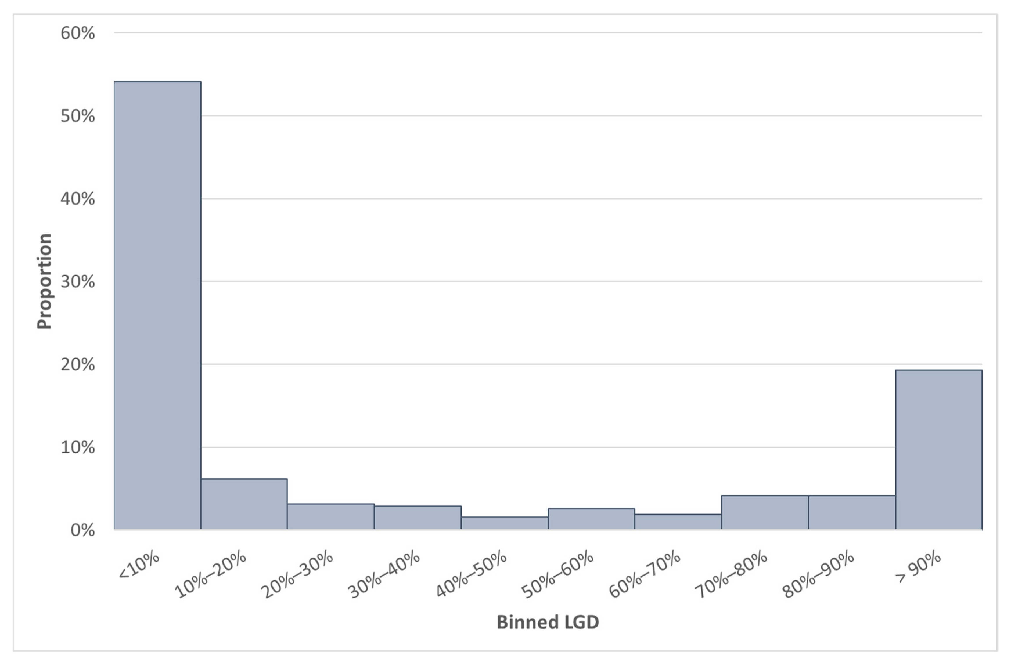
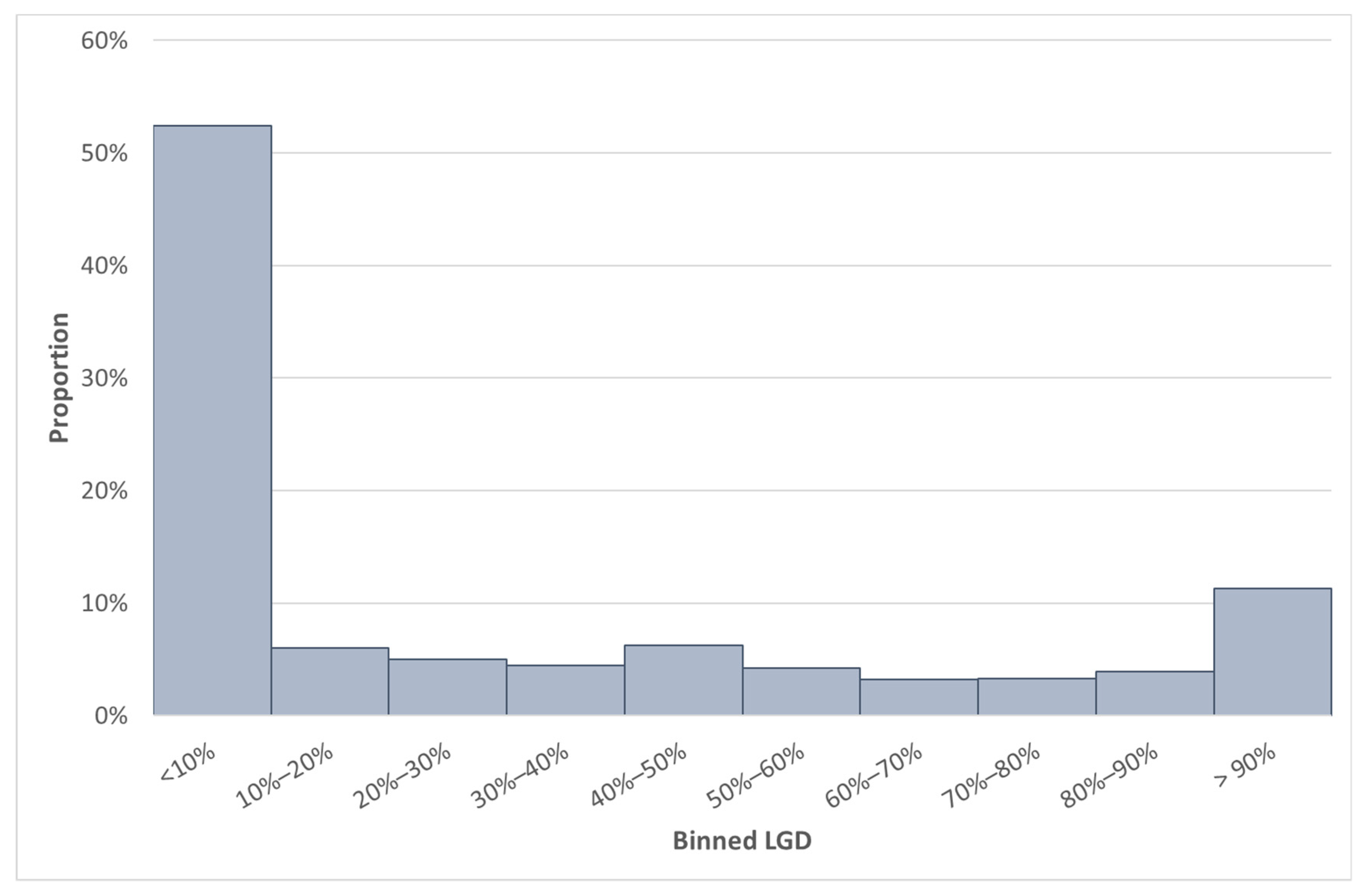
Going forward, we will consider this SA GCD LGD data set, which contains 3831 observations. Due to the confidential nature of some information in the data set, not all the details can be provided. The difference between the median and average LGD for South Africa was 26.04%. The large difference between the mean and the median can be explained by the bimodal distribution of the LGD data, which is also positively skewed (see Figure 2). Furthermore, the standard deviation of the LGD variable in the SA GCD data set was 0.4. The LGD values of the SA GCD data set are depicted in Figure 2. The typical distribution of LGD is expected to be a bimodal distribution (GCD 2018; Riskworx 2011).
In the GCD data set we used, it is possible to identify the country of origination of a loan, but the identity of the specific bank is protected1. To “synthetically create” a bank’s internal data, we used a 25% random sample from the SA GCD data set, representing a hypothetical SA bank, say ABC Bank. This resulted in a sample of 958 observations from the original 3831 observations in the SA GCD LGD data. The remaining 2873 observations will then be regarded as the data set in question (Data set Q).
The ideal situation would have been to use an actual bank’s internal data and not just a random sample, as described above. This case study, however, aims to illustrate the methodology. We will assume that ABC Bank is considering building a LGD model with only internal data or augmenting their internal data with the pooled data set created as described above. If ABC Bank wants to augment their internal data with this pooled data when developing a regulatory model, they need to assess whether the pooled data set is representative. ABC Bank’s internal data will be the base data (i.e., Data set B), and the SA GCD data will be the data set to be assessed for representativeness (Data set Q). We will illustrate the proposed methodology from the perspective of ABC Bank.
Step 1: Split the base data set (Data set B) into one part for developing a model, namely Data set BB (Base Build), and another part to evaluate the model that was build, say, Data set BT (Base Test).
We split ABC Bank’s data set randomly into an 80% build data set (Data set BB with 767 observations) and a 20% test data set (Data set BT with 191 observations). We will use the Data set BB to build a model (Step 2), and we will evaluate the model performance on the test data set (Data set BT) in Step 4. We will build a second model (Step 3) on the augmented data set (but excluding the test data of ABC Bank), i.e., build a model on Data set Q + BB. This results in 3640 observations, either by calculating 3831 − 191 = 3640 (SA GCD data set less Data set BT) or 2873 + 767 = 3640 (Data set Q + BB). We will evaluate both models on the test data set of ABC Bank, Data set BT (Step 4), as shown in Figure 3.
Step 2: Build a model on Data set BB (Base Build).
A linear regression model was fitted to the build data set of ABC Bank’s data (Data set BB), using LGD as the dependent variable. The underlying assumptions, as stated in Section 4.1, were checked and found satisfactory. Only five of the six predictor variables (discussed above) were statistically significant at a level of 5%. The results are shown in Table 3. One exception was made with the variable Facility type when fitting the model on ABC bank’s data. For this variable, the p-value was 8%, and the variable was not excluded from the regression, since the literature confirmed that the variable is an important LGD driver. Furthermore, in all other analyses (see Table 4 and Section 4.3), this variable (Facility type) had a p-value of less than 1%.
The R-squared statistic was 32.68%. This value indicates that 32.68% of the variance in LGD can be explained by the five variables. The adjusted R-squared statistic was 32.15%. R-squared values in these ranges are not uncommon for LGD models, as evident from Loterman et al. (2012), who reported R-squared values for LGD models in the range of 4–43%.
Step 3: Add the data set in question (Q) together with the base data set (BB) and build a model on this augmented data (Data set Q + BB).
Next, a linear regression was fitted on the Data set Q + BB (this is the SA GCD data set excluding the test data set of ABC Bank and contains 3640 observations). The results of this regression are shown in Table 4. All six of the variables are statistically significant at the 5% level. The R-squared statistic was 32.16%, and the adjusted R-squared statistic was 32.05%.
Step 4: Evaluate the model performance (e.g., MSE) of these two models on the base test data set (Data set BT) and determine whether the model performance has improved or is similar using the following construct.
Step 4.1: Define M S E Q + B B , B T as the MSE of Data set BT using the model build on Data set Q + BB and M S E B B , B T as the MSE of Data set BT using the model build on Data set BB.
The models fitted in Steps 2 and 3 were applied on the test data set of ABC Bank (191 observations, Data set BT), and the MSE results on both the build and test data are shown in Table 5. The first subscript of the MSE indicates the development data set, and the second subscript indicates on what data set the MSE was calculated. The MPAI was also calculated for the instances where the development and test samples were not identical (Taplin and Hunt 2019). When the MPAI is calculated for examples with identical data sets used during model development and testing, the MPAI will be equal to one, as evident in Table 5.
Step 4.2: If M S E Q + B B , B T < M S E B B , B T , the model developed on the augmented data has improved the model performance over the model developed only on the base data.
We observe that the M S E Q + B B , B T is indeed smaller than M S E B B , B T and conclude that the model developed on the augmented data has improved the model performance. Optionally, we could have performed Step 5 to confirm the significance of the difference between M S E Q + B B , B T and M S E B B , B T . The above results imply that, when using the augmented data in the development of the model, improved predictive accuracy of the internal observations (Data set BT) resulted. Based on this argumentation, Step 5 is not applicable in case study 1 due to the outcome of Step 4. We can then conclude that it is safe to continue using the SA GCD data for LGD model development and calibration for ABC Bank. This result is to be expected given the manner in which Data set B was constructed for ABC Bank, i.e., a random sample. The purpose of this case study, however, was to provide a step-by-step implementation guide on how a member bank of an external data provider could use our proposed methodology to assess representativeness.
The results from the MPAI indicate that the average variance of the estimated mean outcome at testing when developing the model using only Data set BB is lower than the average variance of the estimated mean outcome at development. Furthermore, the value of 0.86 is just outside our proposed threshold of 0.9 to 1.1, indicating that further investigation is required. This marginal difference between the conclusion drawn from our proposed technique and the MPAI could be expected as the MPAI was developed for a different objective than our methodology. This is potentially an indication that our proposed thresholds for the MPAI might be too strict, and further refinement might be required. On the positive side, the value indicates that the estimated mean variance of the response at testing is lower than at development. For the model developed on the augmented data (Data set Q + BB), the MPAI of 1.09 indicates that the average variance of the estimated mean outcome at testing is higher than at development but within our proposed range of 0.9 to 1.1, validating our conclusion.

4.3. Results of Case Study 2

In this case study, our proposed methodology is demonstrated with a slightly different aim: we consider which countries in the global GCD data set could be used to augment the SA GCD data in the case of LGD modelling.
Step 1: Split the base data set (Data set B) into subsets, with one subset for building a model, namely Data set BB (Base Build), and another subset to evaluate the model that was build, say, Data set BT (Base Test).
Using the methodology as described in Section 3, we will use the SA GCD data set as the base data set (Data set B) split into an 80% build data set (Data set BB with 3065 observations) and a 20% test data set (Data set BT with 766 observations) to build a LGD model on Data set BB. We will then investigate another country on the GCD data set and append this country’s data (Data set Q) to the SA data set (Data set BB) and build a LGD model. We will evaluate these two models on Data set BT. We repeated this for all the countries available in the GCD data set. We considered 42 countries after the filters were applied based on a threshold of minimum facilities.
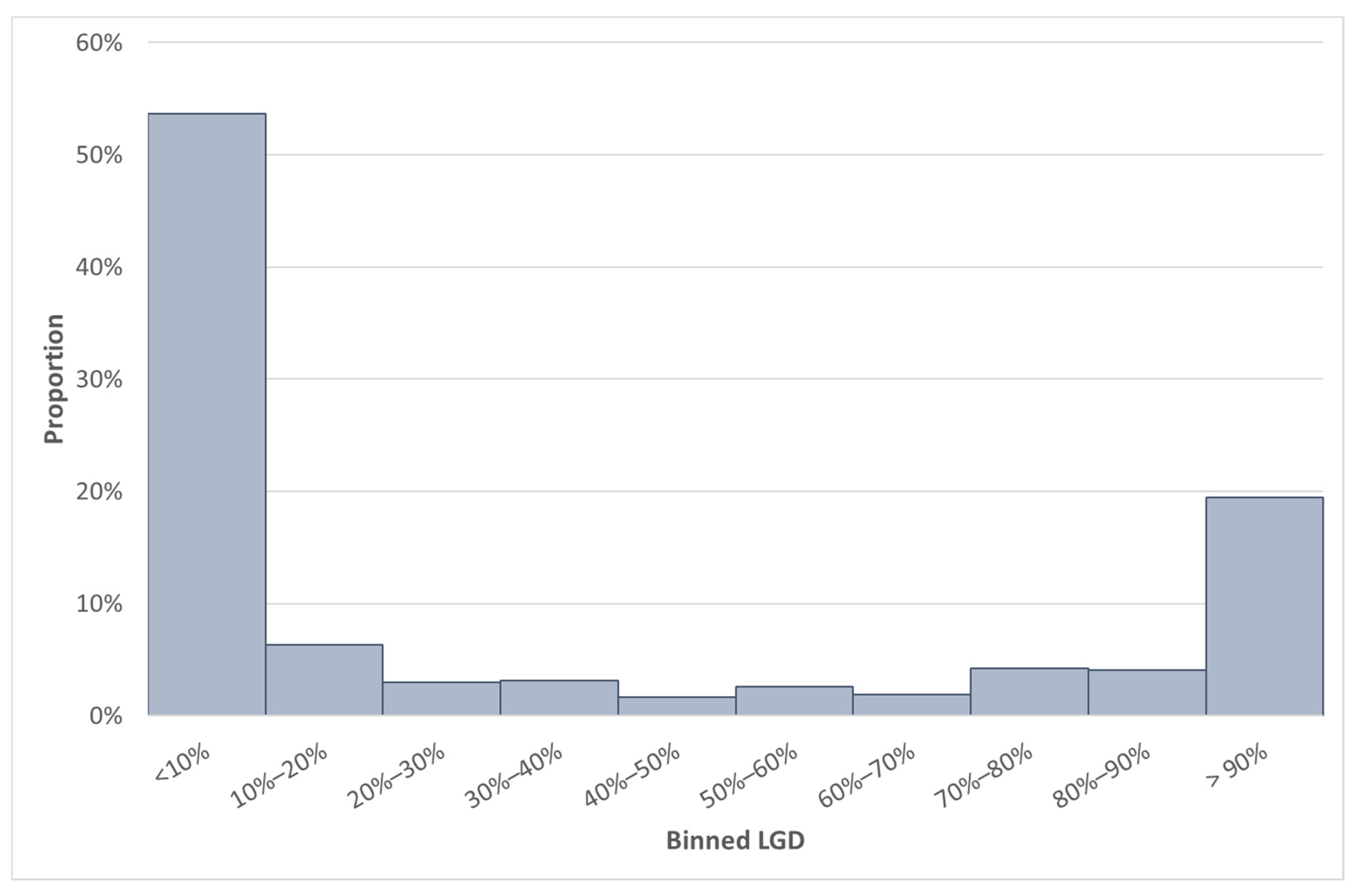
Some summary statistics of Data set BB are shown in Table 6 and the distribution of the GCD LGD value (of Data set BB) in Figure 4.
Step 2: Build a model on Data set BB (Base Build).
A linear regression model was fitted on the SA GCD build data set (Data set BB) after the independent variables were binned, quantified and the resulting binning info was applied to the SA test data set (Data set BT). Once more, all underlying model assumptions were acceptably adhered to. Five of the six variables were statistically significant at the level of 5%. The results are shown in Table 7.
The R-squared value was 32.51%, and the adjusted R-squared value was 32.40%. Note that the results of Step 1 of case study 2 are comparable to the results of Step 2 of case study 1, as both used the SA GCD LGD data set. The difference, however, is that, for case study 1, the test data set of ABC Bank was excluded, and for case study 2, the test data set for SA was excluded.
Step 3: Add the data set in question (Q) together with the base data set (BB) and build a model on this augmented data (Data set Q + BB).
Next, a linear regression was fitted on the augmented data set. The augmented data set is the SA GCD build data set (Data set BB) and one country from the GCD data set (Data set Q). Note that, before fitting a linear regression, the independent variables were binned and quantified on Data set Q + BB, and the resulting binning info was applied to the SA test data set (Data set BT). We repeated this exercise and fitted linear regressions to each of the 42 countries.
We first display the expanded results of two countries: Country L in Table 8 and Country AH in Table 9. The reason for choosing these two countries is because Country L performed the best on the test results and Country AH performed the worst. We then present the abbreviated results of all 42 countries in Table 10.
Considering Country L, the resulting augmented data set contained 3337 observations (3065 from SA build plus 272 from Country L). Five of the six variables were significant at a 5% level. The R-squared value was 28.26% and the adjusted R-squared value 28.14%, as observed in Table 8.
Considering Country AH, the resulting augmented data set contained 21,645 observations (3065 from SA build plus 18,580 from Country AH). All six variables were significant at the 5% level. The R-squared value was 7.42% and the adjusted R-squared value 7.39% (much lower than previous models), as observed from Table 9.
Step 4: Evaluate the model performance (e.g., MSE) of these two models on the base test data set (Data set BT) and determine whether the model performance has improved or is similar.
Step 4.1: Define M S E Q + B B , B T as the MSE of Data set BT using the model build on Data set Q + BB and M S E B B , B T as the MSE of Data set BT using the model build on Data set BB.
The models fitted in Step 2 (one model, Data set BB) and Step 3 (42 models, Data set Q + BB) were applied to the test data set of the SA GCD LGD data (766 observations, Data set BT) in Step 4.
Step 4.2: If M S E Q + B B , B T < M S E B B , B T   0 , the model developed on the augmented data has improved the model performance compared to the model developed only on the base data.
The model developed in Step 2 resulted in M S E B B , B T = 10.64 % , and not one of the 42 models developed in Step 2 obtained MSE values ( M S E Q + B B , B T ) lower than this. However, many of the M S E Q + B B , B T values were closely related to the M S E B B , B T of the model in Step 2.
Step 5: If M S E Q + B B , B T   M S E B B , B T , a dependent two-sample test (by comparing residual statistics) is performed to determine whether the model developed on the augmented data has a similar model performance to the model developed only on the base data. If the test concludes that the M S E Q + B B , B T is not statistically different from the M S E B B , B T , we deduce that the model developed on the augmented data has a similar model performance than the model developed only on the base data.
In this step, we assess whether the model performances were statistically significantly different from one another. We created paired observations for the absolute error and paired observations for the squared error. The normality assumption for the t-test was checked, and both the absolute error and the squared error followed a normal distribution. Using the paired t-test, the observations were compared to see if the average errors were statistically different (i.e., p-value < 0.05). This was repeated for all 42 countries using both error statistics and is shown in Table 10. We also calculated the test statistics and associated p-values for the nonparametric tests (sign test and Wilcoxon signed-rank test). In all cases, similar conclusions followed based on the results of the nonparametric tests, and therefore, the results were omitted from Table 10. Given the results, 12 countries were identified that had a p-value of 0.05 and were greater on both the squared error and the absolute error, together with a MPAI value between 0.9 and 1.1. When considering either the squared error or the absolute error, some more countries were identified that could potentially be used to enrich the base data for model development and calibration. The highlighted cells in Table 10 indicate either the absolute error or the squared error or where the MPAI signifies that the models developed on the augmented data (of these countries) have similar model performances compared to the models developed only on the base data. When focusing on MPAI values less than 0.9 (and greater than 1.1), there is an exact correspondence to our methodology where either the squared error or the absolute error has a p-value less than 0.05. When changing the direction of comparison by inspecting the p-values obtained from our proposed methodology, there are only three countries out of 42 where both the squared error and the absolute error had p-values less than 0.05, with a corresponding MPAI value between 0.9 and 1.1 (i.e., conflicting results between our proposed methodology and the MPAI). This marginal difference between our proposed methodology and the MPAI could be expected, as we have already indicated that the MPAI was developed for a different objective than our methodology.
In summary, when considering the last three columns of Table 10, 12 countries were found to have M S E Q + B B , B T that was not statistically different from the M S E B B , B T , and we deduced that, for these 12 counties, the model developed on the augmented data (Data set Q + BT) had a similar model performance to the model developed only on the base data (Data set BB).
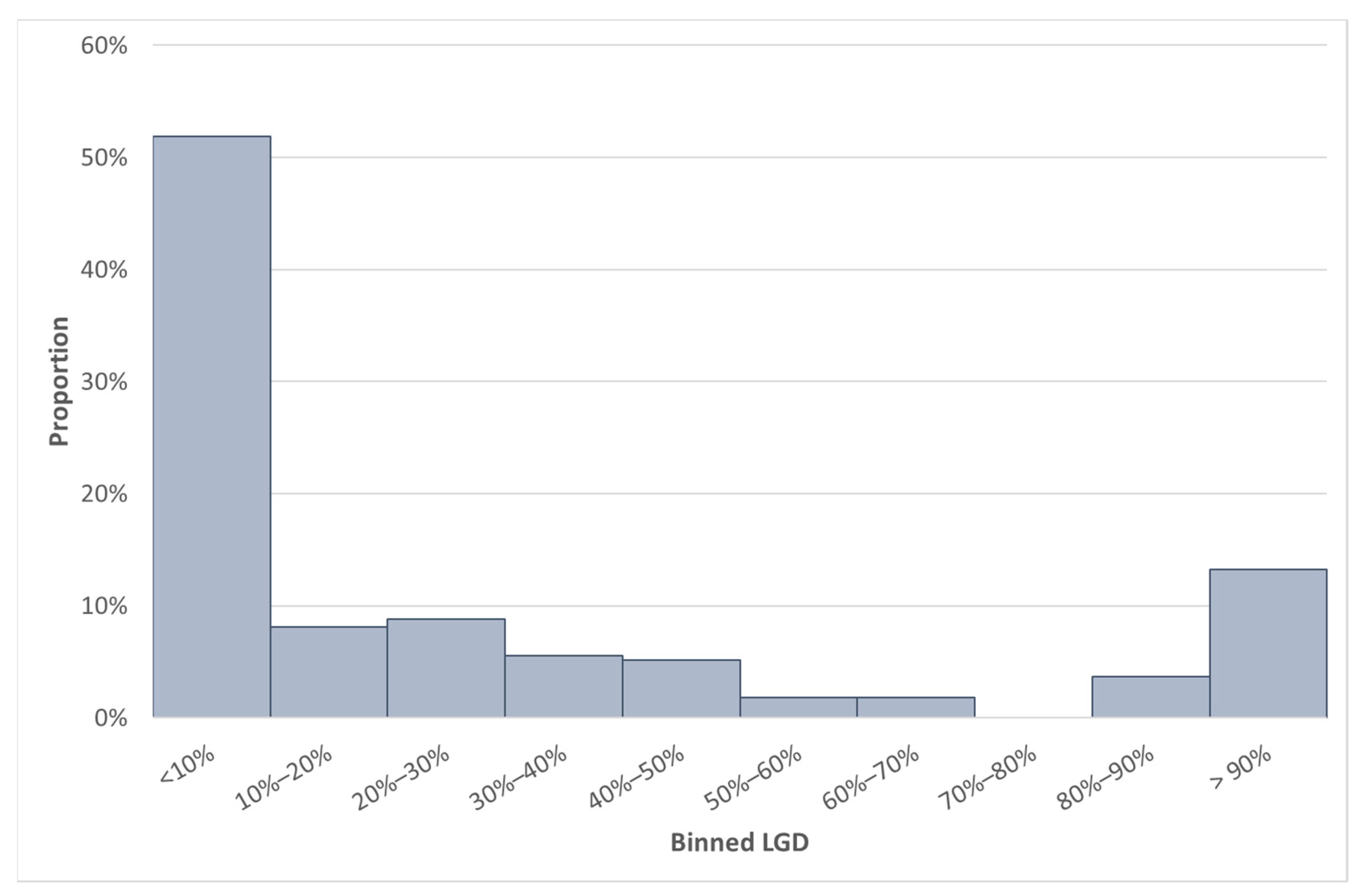
To use our methodology for calibration purposes, it is essential to observe the level of the LGD values. We first focus on Country L (the best-performing Country on the test data set). When comparing Table 11 with Table 6 and Figure 4 with Figure 5, we observed that Country L has a mean LGD value that is more than 10% lower compared to the mean SA LGD. However, the median LGDs of these countries are closely related.
Next, we compare the South African data with the worst-performing MSE. When comparing Table 12 with Table 6 and Figure 4 with Figure 6, we note that Country AH had 18,580 observations. We observed that Country AH has a mean (median) LGD value of 35.3% (7.4%). The mean LGD is lower than the SA mean LGD, but the median LGD are once more closely related.
The summary LGD statistics of all 12 countries that have an absolute and squared error that are not statistically different when compared to the SA data are provided in Table 13.

5. Conclusions and Recommendations

This paper draws together the existing literature on the representativeness of data and classifies these into qualitative and quantitative aspects. Remaining with the quantitative aspects, the paper’s main contribution is the development of a novel methodology that utilises model performance to assess the representativeness of data for model development and calibration. We also evaluated our methodology with the MPAI proposed by Taplin and Hunt (2019), although the original purpose of the MPAI was different from our purpose of testing representativeness.
The proposed methodology uses the following premise: if the model developed on the augmented data (Data set Q + BB) has improved or has a similar model performance (on an out-of-sample subset of internal data) when compared with the model developed only on the base data (Data set BB), then Data set Q is not atypical (i.e., unrepresentative) for model development and calibration. This translates into the belief that it is safe to continue using Data set Q for model development and calibration based on the evidence obtained after executing the proposed methodology.
This proposed methodology was illustrated in two case studies. In case study 1, we investigated whether a pooled data source was representative when considering the enrichment of the internal data with pooled data when developing a LGD model for South African large corporates and SMEs. The results showed that the MSE improved when we augmented the “internal” data with the SA GCD data. We conclude that it would be valid to continue using the SA GCD data for model development and calibration.
In case study 2, we investigated which subsets in the pooled data set could be representative when enriching the data for LGD model development. In this case study, following the application of our proposed methodology, we identified the data of 12 countries that are typical to the base (South African) data when considering the absolute error, squared error and MPAI. More countries could be added if either the absolute error or the squared error is used. Based on the results, we suggest that using the data from these countries is valid when enriching the internal data set to model the LGD. Although these case studies are specific to South Africa, our proposed methodology is generic and applicable to settings unrelated to South Africa, rendering it universally applicable. We also expanded on the proposed thresholds of Taplin and Hunt (2019) when using the MPAI in our research setting. In that regard, we propose two-sided thresholds for the MPAI, taking both improvements and reductions in the average variance of the estimated mean outcome into account. The results showed an exceptional overlap in the conclusions drawn from our proposed methodology compared to the MPAI. The benefit of our proposed methodology is that it is founded on the well-known concept of the hypothesis testing of error statistics.
In terms of future research ideas, we propose investigations into the following:
  • The modelling technique used to illustrate our proposed methodology was linear regression. Many other modelling techniques could be investigated, and it would be ideal to evaluate the performance of our proposed methodology and the MPAI in a simulation design by fitting different models to simulated data and comparing the outcomes under controlled conditions;
  • A similar simulation design could be employed to assess the p-value cut-offs for our proposed methodology and to evaluate the MPAI thresholds proposed by Taplin and Hunt (2019) and those proposed for our setting of assessing representativeness;
  • We used a clustering algorithm to bin industries together, although many other methods exist. A future research study could be to bin the industries using other techniques, such as the classification used by Krüger and Rösch (2017).

Author Contributions

Conceptualisation, W.D.S., C.K. and T.V.; formal analysis, C.K., T.V. and W.D.S.; investigation, C.K., T.V. and W.D.S.; methodology, T.V., W.D.S. and C.K.; software, C.K., T.V. and W.D.S.; validation, C.K., T.V. and W.D.S.; visualisation, C.K., T.V. and W.D.S.; writing—original draft, T.V., W.D.S. and C.K. and writing—review and editing, C.K., T.V. and W.D.S. All authors have read and agreed to the published version of the manuscript.

Funding

This research received no external funding.

Acknowledgments

The authors acknowledge that this research idea benefited from the input of Dries de Wet, and the authors would like to extend their appreciation for these valuable contributions to this manuscript. This work was based on research supported in part by the Department of Science and Innovation (DSI) of South Africa. The grant holder acknowledges that the opinions, findings and conclusions or recommendations expressed in any publication generated by DSI-supported research are those of the authors and that the DSI accepts no liability whatsoever in this regard.

Conflicts of Interest

The authors declare no conflict of interest. The funders had no role in the design of the study; in the collection, analyses or interpretation of the data; in the writing of the manuscript or in the decision to publish the results.

Note

1
A loan from a specific country or region can originate from any global bank that submits data to the GCD.

References

  1. Arlot, Sylvain, and Alain Celisse. 2010. A survey of cross-validation procedures for model selection. Statistics Surveys 4: 40–79. [Google Scholar] [CrossRef]
  2. Baesens, Bart, Daniel Rosch, and Harald Scheule. 2016. Credit Risk Analytics: Measurement Techniques, Applications and Examples in SAS. Hoboken: Wiley & Sons. [Google Scholar]
  3. Barnard, George Alfred. 1974. Discussion of Cross-Validatory Choice and Assessment of Statistical Predictions. Journal of the Royal Statistical Society 36: 133–35. [Google Scholar]
  4. BCBS. 2006. Basel II: International Convergence of Capital Measurement and Capital Standards: A Revised Framework. Basel: Bank for International Settlements, Available online: https://www.bis.org/publ/bcbs128.htm (accessed on 19 January 2018).
  5. Breed, Douw Gerbrand, and Tanja Verster. 2017. The benefits of segmentation: Evidence from a South African bank and other studies. South African Journal of Science 113: 1–7. [Google Scholar] [CrossRef]
  6. Cortés, Lina Marcela, Andres Mora-Valencia, and Javier Perote. 2017. Measuring firm size distribution with semi-nonparametric densities. Physica A: Statistical Mechanics and its Applications 485: 35–47. [Google Scholar] [CrossRef]
  7. Cutaia, Massimo. 2017. Isn’t There Really Enough Data to Produce Good LGD and EAD Models? Edinburgh: Credit Research Centre, Business School, University of Edinburgh, Available online: https://www.crc.business-school.ed.ac.uk/sites/crc/files/2020-11/17-Massimo_Cutaia.pdf (accessed on 15 March 2019).
  8. D’Agostino, Ralph, and Michael Stephens. 1986. Goodness-of-Fit Techniques. New York: Marcel Dekker Inc. [Google Scholar]
  9. de Jongh, Pieter. Juriaan, Tanja Verster, Elsabe Reynolds, Morne Joubert, and Helgard Raubenheimer. 2017. A Critical Review of the Basel Margin of Conservatism Requirement in a Retail Credit Context. International Business & Economics Research Journal 16: 257–74. Available online: https://clutejournals.com/index.php/IBER/article/view/10041/10147 (accessed on 3 December 2020).
  10. Diebold, Francis X. 2015. Comparing Predictive Accuracy, Twenty Years Later: A Personal Perspective on the Use and Abuse of Diebold–Mariano Tests. Journal of Business & Economic Statistics 33: 1. [Google Scholar] [CrossRef] [Green Version]
  11. EBA. 2017. Guidelines on PD Estimation, EAD Estimation and the Treatment of Defaulted Exposures. Available online: https://www.eba.europa.eu/regulation-and-policy/model-validation/guidelines-on-pd-lgd-estimation-and-treatment-of-defaulted-assets (accessed on 18 June 2019).
  12. Engelman, Bernd, and Robert Rauhmeier. 2011. The Basel II Risk Parameters: Estimation, Validation, and Stress Testing, 2nd ed. Berlin: Springer. [Google Scholar] [CrossRef]
  13. European Capital Requirement Regulations. 2013. Regulation (EU) No 575/2013 of the European Parliament and of the Council. Luxembourg: Official Journal of the European Union, Available online: https://eur-lex.europa.eu/eli/reg/2013/575/oj (accessed on 5 December 2019).
  14. GCD. 2018. LGD Report 2018—Large Corporate Borrowers; Reeuwijk: Global Credit Data. Available online: https://www.globalcreditdata.org/library/lgd-report-large-corporates-2018 (accessed on 21 February 2020).
  15. GCD. 2019. Global Credit Data. Available online: https://www.globalcreditdata.org/ (accessed on 5 December 2019).
  16. Hastie, Trevor, Robert Tibshirani, and Jerome Friedman. 2009. The Elements of Statistical Learning: Data Mining, Inference and Prediction. New York: Springer. [Google Scholar]
  17. James, Gareth, Daniela Witten, Trevor Hastie, and Robert Tibshirani. 2013. An Introduction to Statistical Learning with Applications in R. New York: Springer. [Google Scholar]
  18. Joubert, Morne, Tanja Verster, and Helgard Raubenheimer. 2018a. Default weighted survival analysis to directly model loss given default. South African Statistical Journal 52: 173–202. Available online: https://hdl.handle.net/10520/EJC-10cdc036ea (accessed on 5 December 2019).
  19. Joubert, Morne, Tanja Verster, and Helgard Raubenheimer. 2018b. Making use of survival analysis to indirectly model loss given default. Orion 34: 107–32. [Google Scholar] [CrossRef]
  20. Krüger, Steffen, and Daniel Rösch. 2017. Downturn LGD modeling using quantile regression. Journal of Banking and Finance 79: 42–56. [Google Scholar] [CrossRef]
  21. Li, David, Ruchi Bhariok, Sean Keenan, and Stefano Santilli. 2009. Validation techniques and performance metrics for loss given default models. The Journal of Risk Model Validation 3: 3–26. [Google Scholar] [CrossRef]
  22. Loterman, Gert, Iain Brown, David Martens, Christophe Mues, and Bart Baesens. 2012. Benchmarking regression algorithms for loss given default modeling. International Journal of Forecasting 28: 161–70. [Google Scholar] [CrossRef]
  23. Lund, Bruce, and Steven Raimi. 2012. Collapsing Levels of Predictor Variables for Logistic Regression and Weight of Evidence Coding. In MWSUG 2012: Proceedings. Paper SA-03. Minneapolis: Midwest SAS Users Group, Inc., Available online: http://www.mwsug.org/proceedings/2012/SA/MWSUG-2012-SA03.pdf (accessed on 19 January 2018).
  24. Mountrakis, Giorgos, and Bo Xi. 2013. Assessing the reference dataset representativeness through confidence metrics based on information density. ISPRS Journal of Photogrammetry and Remote Sensing 78: 129–47. [Google Scholar] [CrossRef]
  25. Neter, John, Michael H. Kutner, Christopher J. Nachtsheim, and William Wasserman. 1996. Applied Linear Statistical Models, 4th ed. New York: WCB McGraw-Hill. [Google Scholar]
  26. OCC. 2011. Supervisory Guidance on Model Risk Management; Attachment to Supervisory Letter 11-7. Washington, DC: Board of Governors of the Federal Reserve System. Available online: https://www.federalreserve.gov/boarddocs/srletters/2011/sr1107a1.pdf (accessed on 19 January 2018).
  27. Picard, Richard, and Kenneth Berk. 1990. Data splitting. The American Statistician 44: 140–47. [Google Scholar] [CrossRef]
  28. Prorokowski, Lukasz. 2018. Validation of the backtesting process under the targeted review of internal models: Practical recommendations for probability of default models. Journal of Risk Model Validation 13: 109–47. [Google Scholar] [CrossRef]
  29. Prudential Regulation Authority. 2019. Internal Ratings Based (IRB) Approaches (Supervisory Statement SS11/13); London: Bank of England. Available online: https://0-www-bankofengland-co-uk.brum.beds.ac.uk/prudential-regulation/publication/2013/internal-ratings-based-approaches-ss (accessed on 21 February 2020).
  30. Ramzai, Juhi. 2020. PSI and CSI: Top 2 Model Monitoring Metrics. Available online: https://towardsdatascience.com/psi-and-csi-top-2-model-monitoring-metrics-924a2540bed8 (accessed on 1 March 2021).
  31. Riskworx. 2011. LGD Distributions. Available online: http://www.riskworx.co.za/resources/LGD%20Distributions.pdf (accessed on 20 February 2020).
  32. SARB. 2015. Bank’s Act Reporting. Available online: https://www.resbank.co.za/Lists/News%20and%20Publications/Attachments/6864/07%20Chapter%202%20credit%20risk.pdf (accessed on 19 January 2018).
  33. SAS Institute. 2010. Predictive Modelling Using Logistic Regression. Cary: SAS Institute. [Google Scholar]
  34. SAS Institute. 2019. The Modeclus Procedure (SAS/STAT 14.3 User’s Guide); Cary: SAS Institute. Available online: http://documentation.sas.com/?cdcId=pgmsascdc&cdcVersion=9.4_3.4&docsetId=statug&docsetTarget=statug_modeclus_toc.htm&locale=en (accessed on 2 February 2018).
  35. Sheather, Simon. 2009. A Modern Approach to Regression with R. New York: Springer Science & Business Media. [Google Scholar]
  36. Siddiqi, Naeem. 2006. Credit Risk Scorecards: Developing and Implementing Intelligent Credit Scoring. Hoboken: John Wiley & Sons. [Google Scholar]
  37. Sprent, Peter, and Nigel C. Smeeton. 2001. Applied Nonparametric Statistical Methods. London: Chapman & Hall/CRC. [Google Scholar]
  38. Taplin, Ross, and Clive Hunt. 2019. The Population Accuracy Index: A New Measure of Population Stability for Model Monitoring. Risks 7: 53. [Google Scholar] [CrossRef] [Green Version]
  39. Thompson, Steven K. 2012. Sampling, 3rd ed. Hoboken: Wiley. [Google Scholar]
  40. Verster, Tanja. 2018. Autobin: A Predictive Approach towards Automatic Binning Using Data Splitting. South African Statistical Journal 52: 139–55. Available online: https://hdl.handle.net/10520/EJC-10ca0d9e8d (accessed on 5 June 2020).
  41. Wasserstein, Ronald L., and Nicole A. Lazar. 2016. The ASA’s statement on p-values: Context, process and purpose. The American Statistician 70: 129–33. [Google Scholar] [CrossRef] [Green Version]
  42. Yurdakul, Bilal, and Joshua Naranjo. 2020. Statistical properties of the population stability index. Journal of Risk Model Validation 14: 89–100. [Google Scholar] [CrossRef]
  43. Zhang, Yongli, and Yuhong Yang. 2015. Cross-validation for selecting a model selection procedure. Journal of Econometrics 187: 95–112. [Google Scholar] [CrossRef]
Figure 1. Tree-based diagram to define representativeness (across multiple dimensions).
Risks 09 00204 g001
Figure 2. SA GCD LGD distribution.
Risks 09 00204 g002
Figure 3. Visual illustration of the data used in case study 1.
Risks 09 00204 g003
Figure 4. Distribution of LGD of the build data set (Data set BB) used in case study 2.
Risks 09 00204 g004
Figure 5. LGD distribution of Country L.
Risks 09 00204 g005
Figure 6. LGD distribution of Country AH.
Risks 09 00204 g006
Table 1. GCD definition of the asset classes (GCD 2019).
Asset ClassGCD Definition
SMEBorrowers in the Corporate Asset Class as defined in the Basel II Accord §218 and §273, where the reported sales for the consolidated group of which the firm is a part is less than €50 million and where the exposure is not treated as retail, i.e., group exposure > €1 million.
Large corporateBorrowers in the Corporate Asset Class as defined in the Basel II Accord §218 and §273, where the reported sales for the consolidated group of which the firm is a part is above or equal than €50 million but which is not reported in a more specialised Asset Class.
Table 2. LGD values with the associated number of observations for SMEs and large corporates.
SMEsnLarge Corporatesn
LGD < −0.01175LGD < −0.0114
−0.01 ≤ LGD ≤ 1.53600−0.01 ≤ LGD ≤ 1.5231
LGD > 1.50LGD > 1.50
Table 3. Regression results of the ABC build data set (Data set BB).
Parameter Estimates
Variable
(Binned, Average LGD)
Parameter Estimatep-Value
Intercept1.310.02
Facility type0.410.08
Industry code 0.250.02
Collateral indicator 0.59<0.01
Seniority code−4.890.01
Exposure at default0.81<0.01
Goodness-of-fit statistics
R-squared on ABC build data set (Data set BB)32.67%
Adjusted R-squared on ABC build data set (Data set BB)32.23%
Table 4. Regression results of the SA GCD data (Data set Q + BB).
Parameter Estimates
Variable
(Binned, Average LGD)
Parameter Estimatep-Value
Intercept0.590.01
Facility type0.32<0.01
Guarantee indicator−0.400.05
Industry code0.40<0.01
Collateral indicator0.68<0.01
Seniority code−2.52<0.01
Exposure at default0.72<0.01
Goodness-of-fit statistics
R-squared on SA GCD data (Data set Q + BB)32.16%
Adjusted R-squared on SA GCD data (Data set Q + BB)32.05%
Table 5. MSE and MPAI results of case study 1.
MSEMPAI
M S E B B , B B 10.84%1
M S E B B , B T 11.11%0.86
M S E Q + B B , Q + B B 10.70%1
M S E Q + B B , B T 10.78%1.09
Table 6. SA Build data statistics (Data set BB).
Variable: LGD
Number of observations3065
Difference between the mean and median25.94%
Standard deviation0.40
Table 7. Regression results of the build data set of the SA GCD LGD.
Parameter Estimates
Variable
(Binned, Average LGD)
Parameter Estimatep-Value
Intercept2.24<0.01
Facility type0.32<0.01
Industry code 0.44<0.01
Collateral indicator 0.70<0.01
Seniority code−7.91<0.01
Exposure at default0.69<0.01
Goodness-of-fit statistics
R-squared on SA build data set32.51%
Adjusted R-squared on SA build data set32.40%
Table 8. Regression of South Africa GCD build data plus Country L (Data set Q + BB).
Parameter Estimates
Variable
(Binned, Average LGD)
Parameter Estimatep-Value
Intercept0.280.08
Facility type0.40<0.01
Industry code0.46<0.01
Collateral indicator0.68<0.01
Seniority code−2.12<0.01
Exposure at default0.72<0.01
Goodness-of-fit statistics
R-squared on SA plus Country L28.25%
Adjusted R-squared on SA plus Country L28.14%
Table 9. Regression of South Africa GCD build data plus Country AH (Data set Q + BB).
Parameter Estimates
Variable
(Binned, Average LGD)
Parameter Estimatep-Value
Intercept−0.94<0.01
Facility type0.80<0.01
Guarantee indicator0.46<0.01
Industry code0.91<0.01
Collateral indicator0.79<0.01
Seniority code0.66<0.01
Exposure at default0.60<0.01
Goodness-of-fit statistics
R-squared on SA plus Country AH7.42%
Adjusted R-squared on SA plus Country AH7.39%
Table 10. Paired t-test results of the 42 countries.
CountryR-Squared (Q + BB)MSE (Q + BB, Q + BB)MSE (Q + BB, BT)p-Value of t-Test (Squared Error) *p-Value of t-Test (Absolute Error) *MPAI *
Country A29.45%10.77%11.31%0.040.230.952
Country B30.35%10.98%11.11%0.050.040.974
Country C25.75%11.78%11.32%<0.01<0.010.69
Country D28.54%11.11%11.05%0.160.010.983
Country E19.03%10.85%13.08%<0.01<0.010.019
Country F32.02%10.58%10.95%0.710.320.912
Country G29.67%11.07%11.09%0.050.150.983
Country H29.80%11.09%11.14%0.05<0.010.853
Country I28.25%11.22%11.04%0.20.060.9
Country J29.26%11.10%11.19%0.010.011.012
Country K10.56%14.35%13.41%<0.01<0.010.002
Country L28.25%11.11%10.94%0.750.120.905
Country M30.19%10.84%11.04%0.160.160.925
Country N28.49%11.29%11.13%0.02<0.010.9
Country O14.99%9.15%13.85%<0.01<0.010.01
Country P19.58%13.45%13.13%<0.01<0.010.033
Country Q21.86%10.58%13.18%<0.01<0.010.105
Country R27.23%10.96%11.21%0.1<0.010.704
Country S13.96%11.45%13.13%<0.01<0.010.534
Country T30.80%10.62%11.00%0.340.540.914
Country U28.54%11.21%11.10%0.07<0.010.981
Country V14.70%13.67%12.85%<0.01<0.010.052
Country W29.67%11.04%10.97%0.520.280.956
Country X26.44%11.46%11.20%0.02<0.010.874
Country Y31.18%10.78%11.01%0.230.630.933
Country Z22.93%10.37%13.32%<0.01<0.010.047
Country AA28.11%10.89%11.05%0.180.080.912
Country AB14.95%12.53%13.73%<0.01<0.010.772
Country AC16.74%13.37%12.83%<0.01<0.010.099
Country AD29.88%11.09%11.09%0.10.041.013
Country AE15.14%12.60%12.92%<0.01<0.010.515
Country AF25.02%11.87%11.29%<0.01<0.010.752
Country AG28.51%11.36%11.04%0.31<0.010.817
Country AH7.42%11.98%14.27%<0.01<0.010.289
Country AI26.86%11.23%11.09%0.22<0.010.922
Country AJ25.59%10.84%11.12%0.12<0.010.712
Country AK27.74%12.40%11.81%<0.01<0.010.486
Country AL31.24%10.74%10.97%0.310.970.985
Country AM30.61%10.90%11.03%0.080.150.96
Country AN28.31%11.36%11.15%0.04<0.011.023
Country AO29.54%11.18%11.03%0.12<0.010.941
Country AP31.54%10.68%10.97%0.430.340.979
* Highlighted cells indicate either the absolute error or the squared error or where the MPAI signifies that the models developed on the augmented data (of these countries) have similar model performances compared to the models developed only on the base data.
Table 11. LGD summary statistics of Country L.
Variable: LGD
Number of observations272
Mean27%
Standard deviation0.35
Median9.71%
Table 12. LGD summary statistics of Country AH.
Variable: LGD
Number of observations18,580
Mean28.45%
Standard deviation0.35
Median7.47%
Table 13. Summary statistics of the LGD of 12 countries.
CountryMean LGDStandard Deviation of LGDMedian LGD
Country F10.56%0.250.54%
Country G30.31%0.396.71%
Country I29.19%0.384.28%
Country L27.00%0.359.71%
Country M27.48%0.3310.94%
Country T12.61%0.261.08%
Country W27.37%0.381.96%
Country Y29.26%0.368.87%
Country AA21.41%0.313.31%
Country AL19.87%0.314.82%
Country AM23.32%0.374.03%
Country AP17.02%0.303.39%
Publisher’s Note: MDPI stays neutral with regard to jurisdictional claims in published maps and institutional affiliations.

