Efficiency Testing of Prediction Markets: Martingale Approach, Likelihood Ratio and Bayes Factor Analysis


1
Frankfurt School of Finance and Management, Adickesallee 32–34, 60322 Frankfurt am Main, Germany
2
Department of Probability and Mathematical Statistics, Charles University, Sokolovska 83, 18675 Praha 8, Czech Republic
*
Author to whom correspondence should be addressed.
Risks 2021, 9(2), 31; https://0-doi-org.brum.beds.ac.uk/10.3390/risks9020031
Submission received: 1 December 2020
/
Revised: 15 January 2021
/
Accepted: 19 January 2021
/
Published: 1 February 2021
Abstract
:This paper studies efficient market hypothesis in prediction markets and the results are illustrated for the in-play football betting market using the quoted odds for the English Premier League. Our analysis is based on the martingale property, where the last quoted probability should be the best predictor of the outcome and all previous quotes should be statistically insignificant. We use regression analysis to test for the significance of the previous quotes in both the time setup and the spatial setup based on stopping times, when the quoted probabilities reach certain bounds. The main contribution of this paper is to show how a potentially different distributional opinion based on the violation of the market efficiency can be monetized by optimal trading, where the agent maximizes logarithmic utility function. In particular, the trader can realize a trading profit that corresponds to the likelihood ratio in the situation of one market maker and one market taker, or the Bayes factor in the situation of two or more market takers.
Keywords:
prediction markets; efficient market hypothesis; martingale test; likelihood ratio; Bayes factorJEL Classification:
C11; C12; G171. Introduction
The primary focus of this paper is to study whether a given probabilistic opinion is optimal in the sense that it cannot be statistically improved by an alternative probabilistic opinion. This is a general question that does not require a financial market and we will address this situation in our text as well. We will illustrate this approach for probabilities that are quoted by the markets. Financial markets that trade probabilities are known as prediction markets. They are often used to examine the market participants’ opinion about the probability of a future event, for instance, in sports outcomes or elections. The market prices represented by the quoted probabilities in the prediction markets are expected to already be the best, meaning that alternative views are not expected to generate long term profits. This situation is known as market efficiency in the finance literature. Our paper addresses the case of identifying market efficiency violations and shows how to monetize any possible discrepancies.
The property of efficient markets is that they reflect all currently available information and make an accurate forecast of the price, as shown by Fama (1970). LeRoy (1989) showed that if the information consists of historical prices only, the so called weak-form efficiency, meaning that the current asset prices reflect all information contained in historical prices, equivalent to the martingale hypothesis. We apply this approach using regression analysis for the efficiency testing of prediction markets based on the martingale property. Most importantly, we show the relationship between profits from the optimal trading of an agent that maximizes logarithmic utility and the test statistics based on likelihood ratio and Bayes factor. This leads both to the statistical test and the trading strategy that extracts profits when the markets become inefficient.
Our proposed approach can be summarized as follows. We use prediction market data on soccer that cover the 2016/17 season of the English Premier League. This market’s choice is for illustrative purposes to show how to apply a general theory of statistical testing based on profit statistics, as described in our paper. The advantage of this data set is that it covers a relatively large number of games (362 games with data from the total 380 games in the season) where the probabilities are quoted during the soccer game (in play) with the frequency of one minute updating. We split the data set into a training part of the first 262 games and a testing part of the remaining 100 games. This would allow an agent to spot any market efficiency violations in the training data and extract the potential profits in the testing part of data in real trading.
To identify any possible violation of the market efficiency hypothesis, we run a linear regression analysis, where the explained variable—the outcome of the game in terms of a binary 0-1 variable—is regressed on the quoted market probabilities. In efficient markets, the best predictor of the outcome should be the last quoted price. The quotes of the previous prices should be statistically insignificant. The regression analysis leads to two conclusions. The first one is to identify the possible pairs of time indices with , where the quoted price at time s is statistically significant. This is done on a training set of data, split from the remaining testing set of data. This would indicate a possible violation of the efficient market hypothesis for the specific pair of times . The second outcome of this analysis is that the regression analysis run on two time indices can lead to a different estimate of the outcome compared to the estimate in terms of the last observed quoted probability. The discrepancy between the estimate obtained from the regression analysis and the last quoted price is expected to be greater for pairs , with greater significance of the regression coefficient at time s. In this case, the quoted price at time s would be more influential in terms of the estimate of the outcome, which agrees with the violation of the market efficiency hypothesis.
Once we have two probability opinions—one from the regression analysis and one quoted by the market—we can set a trading mechanism that would confront these two alternative probability distributions in trading. We assume that the market taker, the agent with an alternative probabilistic opinion, maximizes the logarithmic utility function. It turns out that the optimal trading strategy follows a well known Kelly strategy. As a result, we show that this trading strategy’s resulting profit is proportional to the likelihood ratio, thus linking a statistical measure used for hypothesis testing to the realized profit. We apply this trading mechanism on the testing data set to see whether the profits indeed monetized for the pairs of time coefficients that were suspected to violate the market efficient hypothesis. Kelly’s betting strategy dates back to a 1738 article of Bernoulli that was later reprinted in Bernoulli (1954). The same question in a more modern setting was studied by Kelly (1956). A more recent paper Vecer (2020) extends Kelly’s results to an arbitrary number of possible outcomes (even infinite). In contrast to this paper that studies discrete time evolution of the prices, Vecer (2020) focuses on the case of continuous time finance, where the price evolution is driven either by Brownian motion or Poisson process.
The above approach applies directly to a market maker’s situation, which is represented by the quoted price, and the market taker, which is represented by the alternative probabilistic opinion. However, we may have a situation when we have two (or more) probability opinions and no market maker. This happens in various applications outside the prediction markets, for instance, in finance (default probabilities), epidemiology (probability of contracting a particular disease), or in other fields. In this case, the market maker’s role can be played by an equilibrium of the market takers, which happens to be a mixture distribution. The resulting wealth of the agents updates in a Bayesian fashion, which directly links this procedure’s profit to a Bayes factor used in model selection. We also illustrate this approach to our testing data set. It is important to stress that while the market constructed here is hypothetical, the resulting trading profits can still be used as a statistical comparison of alternative probabilistic models. The Bayes approach to hypothesis testing is a traditional area of statistics; see, for instance Jeffreys (1935) and Kass and Raftery (1995).
The traditional time martingale test is based on the idea that the current prices are the best predictors of an event’s outcome given all prior information. In particular, the only significant predictor of the ultimate outcome should be the last observed value. The martingale prediction property should hold as well for the price process observed at any stopping time, which leads us to introduce a novel martingale test based on the first time when the price reaches a certain threshold. Again, we can test whether the quoted probability that corresponds to reaching any previous thresholds is not significant, otherwise the martingale property would be violated.
The spatial martingale test is motivated by the prediction markets standard calibration test, which examines whether contracts priced at a certain level, say , win in fraction of the cases. This can be tested by comparing the market prices against the win frequencies. In an efficient market, the quoted price in terms of probability should correspond to the win frequency. A detailed overview of the application and research topics of the prediction markets literature can be found in Horn et al. (2014). Our approach differs in that we only take the first value above a certain threshold into account, which corresponds to the price process evaluated at the stopping time of reaching the threshold. Therefore, we test whether contracts are priced efficiently at the stopping time, meaning after exceeding a certain threshold for the first time.
We apply the time and spatial martingale tests to football betting data that represent a particular case of prediction markets to illustrate our proposed methods of model comparison that apply to all prediction markets. Due to the high liquidity of such markets, they offer several advantages in the environment of efficiency and martingale testing (see also Croxson and Reade 2014). A football match has a clearly defined outcome and the probabilities extracted from in-play odds converge to the terminal values during a short and fixed period of time. The data are clean and immediately update to all relevant information during the game, which can be easily observed (for instance, goals, penalties or red cards). In comparison to laboratory experiments, the betting market is a real market with motivated and experienced participants. Finally, compared to elections, we have multiple similar prediction markets within a short period of time, namely 380 matches (prediction markets) per one English Premier League season.
We use a straightforward strategy for testing efficient market hypothesis on our market data. We identify all possible pairs of time indices, where the previous quote probability is significant in the regression analysis on the training data and use the new prediction to test it in trading on the testing data. We choose 5% and 1% significance levels. As a comparison, we also take all predictions from the regression analysis, regardless of the statistical significance of the previous coefficient. While we get a relatively large set of possible candidates with high significance based on the training data, it leads mostly to losses when confronted by the last quoted price in the testing data set. This suggests that the training data’s apparent significance has mostly no predictive power and corresponds to random fluctuations rather than some valuable information.
This paper contributes to the field of testing for efficiency and accuracy of prediction markets. From an application point of view, the literature can be divided into prediction markets for political and sport events. In the political prediction market literature, Leigh and Wolfers (2006); Sjoeberg (2009); Wang et al. (2015); Vaughan Williams and Reade (2016) and Brown et al. (2019) analyze efficiency and accuracy of prediction markets compared to opinion polls. Graefe et al. (2014) and Rothschild (2015) study the predictive power of prediction markets combined with opinion polls and Huberty (2015) use social media content to forecast the outcome of elections. More recently, Chen et al. (2019) employ deep learning techniques to study inefficiencies of stock markets. Our paper shares the research direction as in Page and Clemen (2013), who analyze the accuracy of the prediction market over time. Their main finding indicates that accuracy and efficiency improve over time.
The sports prediction market’s literature can be divided into two parts. The first group represents papers that use low frequency data before starting the match and prematch probabilities. Golec and Tamarkin (1991) and Gray and Gray (1997) test for efficiency in the NFL betting market using regression models and apply it to the final price before the start of the match. Vaughan Williams (2005) provides a comprehensive literature review of related papers. The second group of papers analyzed the efficiency of high frequency in-play data that became recently available from betting exchanges. Gil and Levitt (2007) test for efficiency in in-play odds of the Football World Cup 2002 matches. They report that the odds do not update immediately to the arrival of goals and interpret this as evidence of inefficient markets. Page (2012) reveals that the in-play odds are not efficient during the final minutes of a match, as they overestimate the likelihood of low probability outcomes. Our paper focuses on topics previously studied by Croxson and Reade (2014), who test for semi-strong form efficiency in in-play betting odds. They run regression analysis to test for the efficiency of the implied probabilities after goal arrivals. We contribute to the existing literature by introducing a novel approach for efficiency testing for prediction markets based on a spatial martingale test.
The paper is structured in the following way. Section 2 documents martingale tests based on both the time and spatial evolution of the quoted probabilities. We apply these results to the training data set. The martingale tests provide two results; one is an indication of the possible violation of the efficient market hypothesis, the other being an alternative probabilistic opinion based on the regression analysis. Section 3 shows how to confront the new opinion and the market opinion for a market taker that maximizes the logarithmic utility function. The resulting profit and loss distribution corresponds to the likelihood ratio, which provides a nice link between statistics and finance. Our studied market of football betting does not indicate any substantial profitable trading opportunities, which is in fact, an expected result. However, we show how to construct profitable betting strategies on a simulated example that violates the market efficiency hypothesis. Section 4 shows how to confront opinions when no market exists and all market agents are market takers. In this case, the market maker’s role is played by the equilibrium distribution of the market takers. The trading profits from this procedure correspond to Bayesian updating.
2. Results
Let us start our analysis with martingale tests based on regression analysis. Given a process , the martingale property requires that
for , and more specifically, when is the sigma algebra generated by the process :
The linear regression analysis gives the conditional expectation in terms of a linear combination of ’s
Should the result of the linear regression correspond to the martingale, the coefficients should be statistically zero for and should be statistically one. This leads to the following hypothesis test:
Variants of this test have appeared in the previous literature, see for instance Croxson and Reade (2014). In our own text, we limit ourselves to perform this test only for two observations at times , . Our primary focus is not on finding the exact time pairs for which the martingale hypothesis was violated, as this could happen randomly, and no profitable trading strategy could have ever existed, even when we find a violation of this hypothesis in retrospect. Instead, we use this approach on the training data set as a possible indication of the market inefficiency, get an alternative prediction of the outcome based on the regression analysis and use the resulting optimal trading strategy to see if the corresponding trading profits are statistically significant.
In our situation, we linearly regress the market’s outcome in terms of a binary 0-1 variable on the presently quoted probability and the past quoted probability. The previously quoted probability should be statistically insignificant. A significance of this variable would indicate a possible violation of the market efficiency hypothesis. Moreover, the regression analysis gives an alternative probabilistic opinion of the outcome, based on two predictors in terms of the past quoted probability and the currently quoted probability. This new estimate will be used in the following text to test whether the alternative probabilistic view could be monetized. Note that while it could be more natural to use non-linear regressions such as logit or probit on the binary outcome, the non-linearity of these methods would prevent us from the straightforward application of the martingale test.
2.1. Time Martingale Test
The time martingale test examines whether the probability time series follows a martingale evolution. More precisely, we test whether the current market price quoted as a probability is the best estimate for the market’s outcome, given all prior market prices. This can be formulated as
where is the probability quoted by a prediction market for the contract type , market and time . The final observation, , is a binary variable on the outcome of the market, which is one if the event of contract on a prediction market occurs, and zero otherwise. If Equation (5) does not hold, there should exist a profitable trading strategy in the form of buying a contract at a specific point of time and holding it until the end of the event traded on the prediction market.
The test is related to the work of Croxson and Reade (2014), but it differs in two points. First, we use the outcome of the market as a dependent variable. This allows us to test whether the current probability is the best estimate for the outcome and not only the best estimate for the probability at the next time step. Second, we estimate different parameters for different contract types on the same prediction market, to avoid problems caused by a possible dependence between the contracts. Summing up, we estimate different parameters for all combinations of times to test whether the current probability is always the best estimate for the outcome, given all previous probabilities.
The market efficiency test can be performed by estimating the parameters of the following regression model:
with . We run regressions for all combinations of t and and estimate the parameters and . Therefore, we can test whether the probability at time t is the best guess for the outcome, given all previous observed probabilities at times s. Under the null hypothesis that the probabilities satisfy the martingale properties, coefficient should be statistically insignificant.
2.2. Spatial Martingale Test
The spatial martingale test is motivated by the standard calibration test used in the prediction markets literature (see Horn et al. (2014)). In the efficient market, the quoted probability should correspond to the observed frequency. Our approach differs when we take into account only the first observation when the probability is above a certain threshold. This corresponds to evaluation of the process at a stopping time. Therefore, we test whether contracts are priced efficiently after exceeding or jumping above a certain threshold for the first time. Comparing the quoted probability with the frequency of the outcomes is also problematic in the context of football probabilities, as the evolution of the odds can experience dramatic jumps due to goals and some probability levels may never be attained during the game, even for all contracts (win, loss, draw) combined. Thus, the first hitting time is more appropriate for our problem.
The novel spatial martingale test examines whether probabilities that exceed a certain threshold for the first time are the best estimate for the outcome, given all probabilities that exceed lower thresholds for the first time. Practically, this test examines whether there exists a profitable trading strategy like buying a contract that exceeds a threshold for the first time and holding it until the end of the match.
Before we can perform the regression test, let us define as the probability observed at the hitting time , where is given as the first point of time that is outside the interval :
with . We can subsequently arrange the probabilities from the smallest to the highest threshold level. Hence, we transform the time series with into a stochastic process with an increasing . The first value of the new process is the initial probability of the time series, the second value is the first observation that is outside the interval , the third value is the first observation that is outside the interval , and so on. Note that can be zero for some s.
Now, we can test whether probabilities that exceed a certain threshold for the first time are the best estimate for the outcome, given all probabilities that exceed lower thresholds for the first time. This can be formulated in the following way:
where is the probability at the hitting time of contract , market and time . Moreover, is a binary variable on the outcome of the market, which is one if the event occurs, and zero otherwise.
In the spatial martingale regression test, we use the final result as a dependent variable and , as well as as independent variables in the regression model,
with .
We run separate panel regressions for all combinations of and and estimate the parameters and . Under the null hypothesis that the probabilities satisfy the martingale hypothesis, coefficient should be statistically insignificant.
2.3. Application on Soccer Data
As an illustration of our approach, we examine betting data from Betfair for the English Premier League. The English Premier League is one of the most popular football leagues globally and an important market for the online betting industry. Each season of the English Premier League plays 380 matches, where 20 teams play each other twice, once at home and once away. A match consists of two 45 min periods separated by 15 min break plus some extra injury time. Each game has a clearly defined outcome (home win, away win, or draw), based on the home team’s and away team’s final score. During the 15 min break, the odds are typically constant, as there is usually no information update. Thus, we remove the 15 min break to avoid multicollinearity issues in the regression analysis.
We focus on the most liquid market—the outcome of the game. The market offers 3 contracts: home win, away win and draw for every single match of the English Premier League season and they are quoted even during the actual game, which is called in-play. The contracts are traded in real time and are quoted in terms of odds 1 : x. It is possible to buy an event for $1 and receive $x if the event occurs and $0 otherwise, see for instance Vecer et al. (2009). These odds can be interpreted as the probability that the event occurs, see for instance Wolfers and Zitzewitz (2006).
We use the in-play minute-by-minute odds for 362 of the 380 matches of the English Premier League season 2016/17 provided by Betfair. We split the data set on 262 training and 100 testing matches ordered by date, so that an agent who would spot a violation in the market efficiency hypothesis in the training data would monetize this information in the testing data. Moreover, we separate the data into three datasets based on the three events of home win, away win and draw. Finally, for the time martingale test, we cut off the odds after minute 94 to have well balanced datasets. On the other hand, we do not cut off the probabilities after for the spatial martingale test and use all available probabilities when calculating the hitting times.
As for the independent variable, we transform the Betfair odds 1 : into probabilities . We set to represent the events of the home win, the away win and the draw, where indicates the match index and the in-play minute-by-minute time. The probabilities of the three events should add up to one for a given match and time. However, although the markets quote the odds with only a tiny margin, we need to adjust the odds correspondingly. Therefore, the relationship between the odds can be expressed by
where is the market margin. The probabilities of the three different events can be calculated using the following formula:
For the dependent variable, we use the final score of each match in our analysis. These data are provided by the official Premier League website, https://www.premierleague.com/results. We define the final result of each contract (home win, draw, away win) based on the final score of each match , whereas and represent the number of goals of team home and team away:
Finally, we have three different panel datasets for every contract type , namely the home win, the away win and the draw, each with 362 matches and 95 time steps , as well as the final results for all three contracts and 362 matches.
The time martingale test examines whether the current in-play probability is the best estimate for the outcome of the match, given all prior probabilities. This is tested by the regression model (6),
where is the probability extracted from the football betting odds of a contract , match and time . Moreover, is a binary variable on the outcome of the match , which is one if the event of contract occurs and zero otherwise. Under the null hypothesis that the probabilities satisfy the martingale properties, the second coefficient should be insignificant.
We estimate the coefficients of the time martingale regression model to test for the efficiency of the time series data using the Premier League 2016/17 minute-by-minute data with . We run 4465 regressions for each of the three events (home win, away win and draw), as we have 4465 possible combinations of t and . Under the null hypothesis, the second regression coefficient should be insignificant for all combinations of t and . We report the results of the regressions in Table 1 and in Figure 1. Table 1 lists the number of instances when the second coefficient is significant on 5% and 1% p-values.
Figure 1 visualizes the results of the regression analysis. The graphs represent the p-value of the second regression coefficient in home, draw and away betting markets. Every colored point represents the p-value of a different regression and is the combination of at time t on the y-axis and at time s on the x-axis. Yellow color represents p-values close to 100% and blue color represents p-values close to 0%.
The home win data results indicate that 110 (2.46%) of the second regression coefficients are significant at a 5% level and 20 (0.45%) are significant at a 1% level. Having a closer look at the significant coefficients shows that regressions with parameters t and s after the break and close to the end of the match are significant. The draw data set results show that 75 (1.68%) of the second regression coefficients are significant at a 5% confidence level and 12 (0.27%) at a 1% confidence level. As we illustrate in the following section, the p-value significance in training data results from random fluctuations and does not have any predictive power for the testing data set. The p-values of the away win data show similar results 840 (18.81%) of the coefficients are significant at a 5% level and 363 (8.13%) at a 1% level. Again, the regression models with parameters after the 15-minute break show significant second regression coefficients.
The spatial martingale test examines whether probabilities that exceed a certain threshold for the first time are the best estimates for the outcome given all probabilities that exceed lower thresholds for the first time. This can be tested by estimating the coefficients of the following regression model (9),
where is the probability at the hitting time of a contract , match and time . Again, is a binary variable on the outcome of the match, which is one if a specific event occurs and zero otherwise. Under the null hypothesis that the probabilities satisfy the martingale properties, the second coefficient should be insignificant.
We estimate the coefficients of the spatial martingale model to test for efficiency of the spatial process using the Premier League 2016/17 minute-by-minute data with thresholds . The possible combinations of and , with , result in 1225 regressions. Under the null hypothesis, the second regression coefficient should be insignificant for all combinations of and . We report the results of the regressions in Table 2 and in Figure 2.
Table 2 shows the number of p-values that indicate significant second regression coefficients at a level of 5% and 1% and the number of p-values of the second regression coefficient that are below the 5% and 1% confidence level of the comparable p-value distribution. Figure 2 visualizes the results of the regressions. The graphs show the standard p-values of the second regression coefficient for the home, draw and away markets. Every colored point represents the p-value of a different regression and is the combination of with the threshold on the y-axis and at time on the x-axis.
The home win data set results show that 35 (2.86%) of the p-values indicate a significant second regression coefficient at a 5% significance level and 9 (0.73%) at a 1% significance level. More specifically, regressions with combinations of high and show p-values below 5%. This is due to the momentum of the game. High values of and indicate that the probability of winning is either very high or very low. The observed high significance of the regression coefficient corresponding to means that all the games in our training set that entered 95% probability before reaching 99% probability of winning all resulted in a win and the games that entered 5% probability before reaching 1% probability of winning all resulted in a loss. This can easily happen, as we have 262 games in our training set and the probability of a game reversal at this stage is only 1%.
The probabilities of of the draw data set for are almost constant. The reason is that the initial quotes of the probability of the draw are typically below 30%. Thus, we limit ourselves to run 1035 regressions with the parameters and . The results are in line with our previous findings. The second regression coefficient is significant 48 times (4.64%) at a level of 5% and 42 times (4.06%) at a level of 1%. The second regression coefficient is almost always significant at a 1% level for regressions with . This is a similar phenomenon to the case of the home team win. It turns out that all games that reached 99% probability threshold ended up in win in this market and the games that reached 1% probability threshold ended up in loss in this market. Thus, we see significant coefficients of the previous quotes when in Figure 2 in the draw market, which corresponds to the bottom horizontal line. The significance of the previous coefficient corresponds to a momentum trading strategy. Meaning buy the bet when it reaches 99% and sell the bet when it reaches 1%. Such a strategy has a 99% success rate to start with, so this can easily happen, but drawing conclusions about the statistical significance of this trading strategy on a relatively small data set (262 games) is not appropriate as a single exception to this rule would ruin both the significance of the second regression coefficient and profitability of this trading strategy.
The results of the away win data set show that 45 (3.67%) of the coefficients are significant at a 5% level and 38 (3.10%) are significant at a 1% level. We see the same behavior of statistical significance of the second regression coefficient when , which is again caused by the fact that there was no game reversal when the market reached 99% or 1% probability quote.
3. Realized Profit as a Statistical Measure of Model Comparison, Link to Likelihood Ratio
The previous section answers whether the quoted probabilities satisfy the martingale property or not required for the efficient market hypothesis. Suppose that the analysis concludes that the markets are inefficient, meaning that we can construct better predictors of the outcome based on the historically observed data. The following text shows how one can optimally extract the profit from such observed discrepancies having a different view about the prices than quoted by the market.
A general setup of this problem is to consider two agents; one is a market maker with a probability measure and one is a market taker with probability measure . The market taker’s question is what would be the optimal betting strategy that would maximize the expected utility of the resulting profit. This problem mathematically means to find the optimal payoff F for a given utility function U that maximizes
under the constraint
The maximization part of this problem is clear; what is less obvious is the constraint on the zero expectation of the market. The prediction market quotes the price q for an outcome X with a binary 0-1 payoff, with
being the price of the contract. Such contracts with binary payoffs are known in finance as Arrow–Debreu securities. Thus, the realized profit of any such trade scaled with an arbitrary volume V is in expectation simply
The betting markets are analogous with the difference that the market quotes the betting odds as
with the payoff on win and on loss. The expectation of such a bet X is
The prediction markets usually allow for both negative and positive positions, so the market taker can indeed construct, in practice, an arbitrary payoff F satisfying the condition . The betting exchanges, such as Betfair, also typically allow for negative betting positions, which makes the condition of constructing the payoff with a zero expectation from the perspective of the market applicable. In the case of a binary outcome, one can construct all possible payoffs with zero market expectation, even under the constraint of positive bet size by betting on one of the two available outcomes. We assume zero market overhead, which can be translated in financial terminology as zero transaction costs.
This problem of maximizing the expected utility of the payoff F under the market taker’s measure with the constraint on zero market expectation of such payoff has been recently considered in this form in Vecer (2020) and solved for an arbitrary random outcome and an arbitrary utility function U. The following theorem summarizes the general result:
Theorem 1.
The optimal payoff F that maximizes under the constraint is given by
where and where λ solves
Proof.
The constrained optimization problem is to consider the following Lagrange type functional
The optimal F solves
giving
which leads to
where
and where solves
□
The most interesting link between the profit size and traditional statistics happens for the logarithmic utility function in the form
where B is a parameter representing the agent’s bankroll. For this choice of utility, the optimal payoff position is
The random variable F represents the trading profit after observing the outcome . The market taker realizes profits on subjectively more likely outcomes and losses on subjectively less likely outcomes than quoted by the market. The bankroll B updates to
Example 1.
Consider a binary random variable X and an agent with an initial bankroll . The market quotes
The agent believes
The optimal payoff for the marker taker is a random variable
The updated bankroll becomes
Assume that the agent starts with a bankroll B and uses the above betting strategy to maximize the logarithmic utility. In this case, her terminal bankroll becomes
which is a likelihood ratio. In statistics, this is a fundamental concept used for hypothesis testing, which dates back at least to Neyman and Pearson (1933).
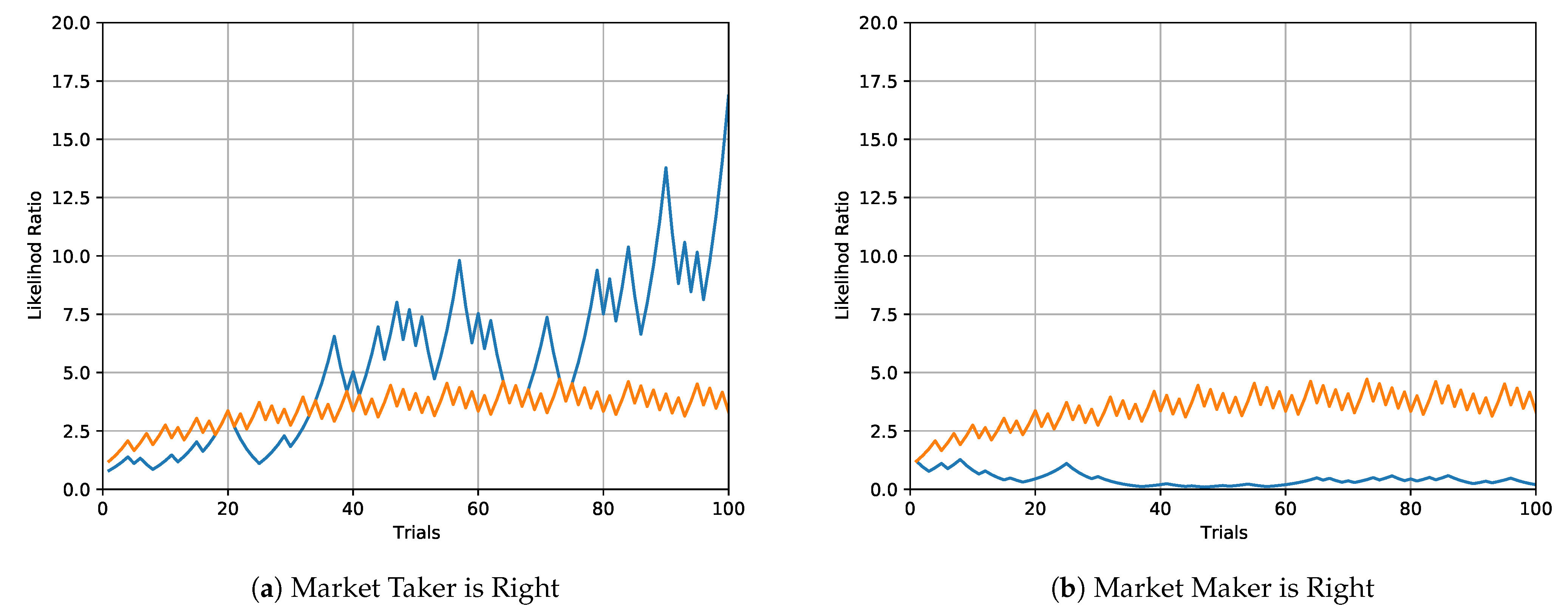
Figure 3 illustrates the optimal trading in two situations when the market taker starts with a bankroll . The first situation is when the opinion of the market taker is correct and the market maker quotes incorrect probability. In this case, the wealth of the market taker becomes quickly statistically significant. The second situation is when the market maker is correct and the market taker is incorrect. In this case, the wealth of the market taker quickly converges to zero.
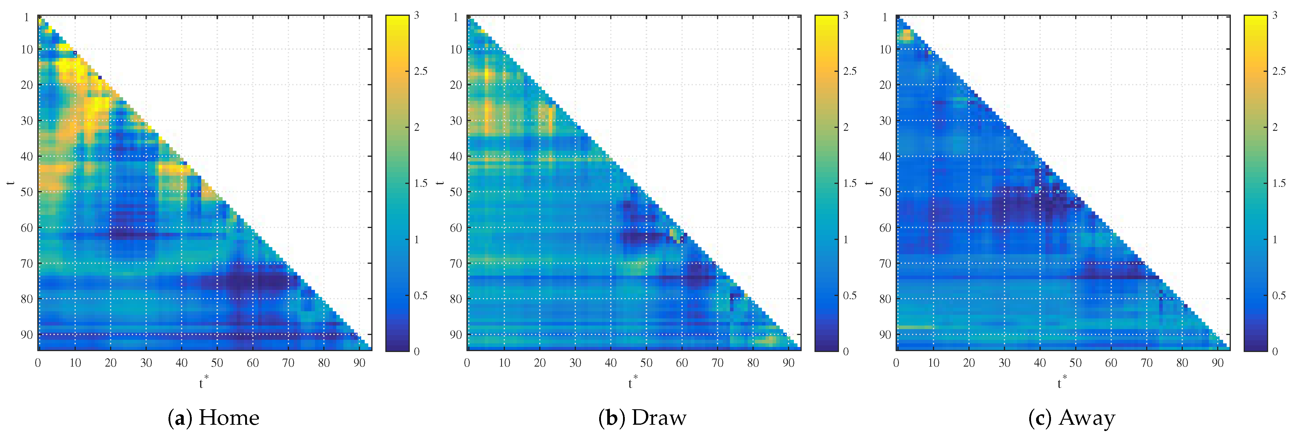
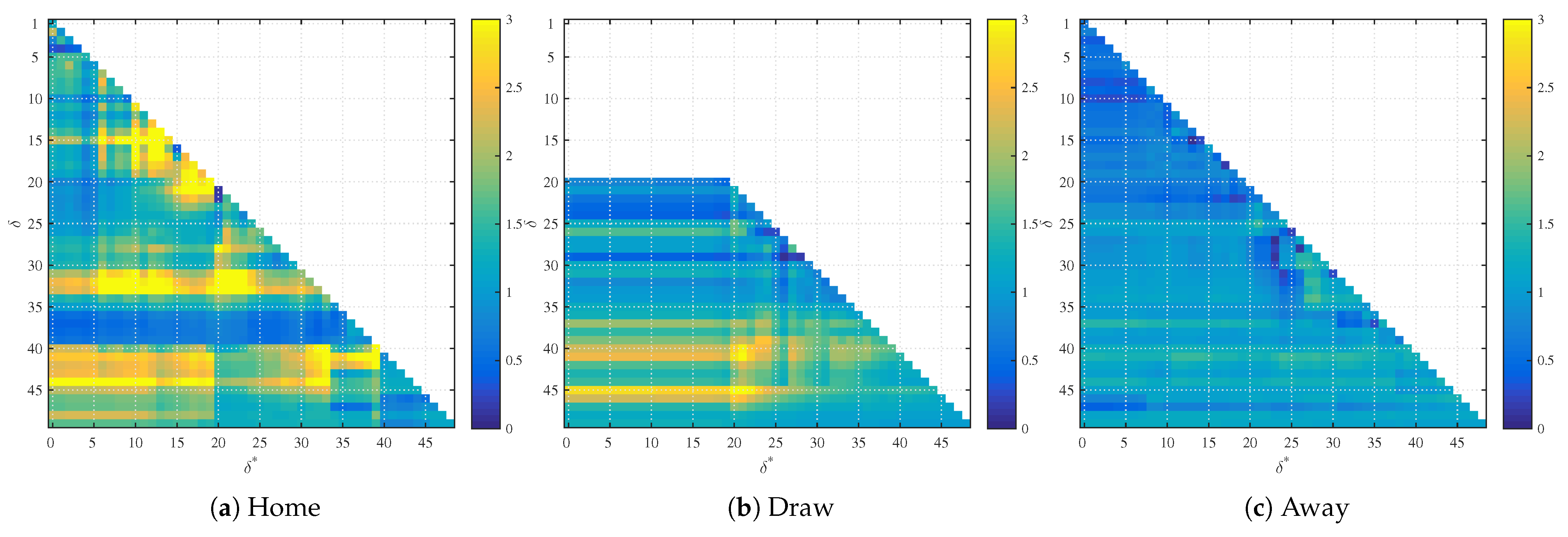
Following the above trading strategy, we can compute the resulting trading profit for each time pair and each market—home win, draw and away win. Without the loss of generality, we set the initial bankroll to . The quoted probability is represented by and the alternative probabilistic view based on the regression analysis on two regressors is represented by . We apply it to the testing part of the data set of the remaining 100 games. While the trading results in the likelihood ratio statistics, these results’ statistical significance is not immediately apparent as the quoted probabilities are not identically distributed. The test’s powers can be simulated from bootstrapping, but this is outside of the scope of our paper. Obviously, the terminal wealth (likelihood ratio) above 1 corresponds to trading profits and below 1 to trading losses. Visually, Figure 4 shows the realized profit of regression models when trading against the quoted probabilities. The yellow color represents profits and blue color represents losses. Similarly, Figure 5 represents trading profits and losses based on the spatial stopping time strategy.
While the Figure 4 and Figure 5 visually show some areas for which the trade uses the probability from the regression analysis, the question is whether such profits are being announced upfront in terms of a statistical significance of the second regression coefficient. We test three basic strategies. The first is to use all the probabilities obtained from the regression analysis and trade them against the market. The second strategy is to use only situations where the second coefficient has a smaller than 5% significance. The last strategy is to use only situations where the second coefficient has a smaller than 1% significance.
Table 3 illustrates the trading results based on trading probabilities obtained from regression analysis against the market for testing data. The results based on time data show that the market realizes profits based in all markets based on time analysis. The result is pronounced even more if we restrict ourselves to more significant coefficients. When we take all possible pairs, the trading result is slightly below one (except for the away market), suggesting that the regression analysis picked up just a random noise with a little negative impact on the trading result. However, if we restrict our set to statistically significant noise, this becomes highly detrimental as the new opinion is away from the market, but the efficient market punishes wrong opinions and thus we see heavy losses for the agent. This suggests that the market is quite efficient.
The agent would be slightly more successful if she followed the spatial betting strategy, exploring trends and reversals in the game as predicted by the regression analysis. For the home and draw markets based on spatial data, the agent would generate profit, but the profit itself is not statistically significant. Restricting the agent to more significant coefficients has a mixed impact, leading mostly to statistically insignificant results. The only statistically profitable strategy is for the away 1% significant markets. This is because 1% significant coefficient corresponds to entering 99% or 1% probability of winning in the market and all the games ended in the projected outcome in the training data set. This is also true for the testing data set, there was not a single reversion of the result. Thus, the agent who would make a bet on the projected outcome with either high or low quoted probability would make a small profit, with high probability in all these 100 games in the testing data set. However, a single market reversal during these games would ruin the profitability and statistical significance of this strategy, as the agent’s loss would be relatively large for this game.
4. Bayes Factor as a Likelihood Ratio
This section considers a situation when two or more probabilistic opinions exist, but there is no market maker that would clear them. This case is more typical, as the prediction markets cover only a small number of specialized interest segments. Thus, the approach adopted here has wider applicability to any probabilistic estimation. When the market maker is absent, its role can be played by an equilibrium distribution of the market takers.
This problem has been recently addressed in Vecer (2020) for a case of a possibly infinite number of market takers. Let the market takers be represented by agents for some state space that can be either finite or infinite. The agents are maximizing individual logarithmic utility, each with a bankroll and with a specific distributional density opinion . We assume that the total bankroll of the market is finite.
The market would be in equilibrium m if the total realized optimal profit for each outcome x is equal to zero:
The equilibrium distribution density is a mixture distribution—a weighted average of the individual densities , where the weights are proportional to the bankroll parameter , as characterized by the following theorem.
Theorem 2.
The equilibrium density is given by
where is the total bankroll of the market.
Proof.
This follows from the fact that the equilibrium density on the outcome x satisfies
which is equivalent to
and thus
□
The paper of Vecer (2020) shows in detail that the agents’ bankrolls evolve in a Bayesian fashion. If one thinks about the initial bankrolls as the prior distribution, the equilibrium distribution is an unconditional distribution and the updated bankrolls after observing the outcome of the trade are posterior distributions. Without repeating in detail these results, let us show how the bankrolls evolve in a model with just two probabilistic opinions, say and .
Assume that the two agents have initial bankrolls and with , so that the total bankroll of the market is scaled to one. The first argument represents the model’s index, the second argument represents the number of observations of the outcome. The resulting market equilibrium on outcome x is
This represents the market price where the opinions of market takers clear. The agent realizes profit on outcome
The updated bankroll becomes
This result has a Bayesian interpretation. Let represents the prior distribution . The probability opinions represent likelihood function, , while the equilibrium distribution corresponds to
which is the unconditional distribution of the outcome . The updated bankroll is the posterior distribution
By repeating this procedure, the size of the updated bankroll corresponds to the posterior probability
This can be regarded as a likelihood ratio similar to Equation (19), but between probabilistic measures and the equilibrium measure , which represents unconditional probability. The equilibrium measure keeps the updated bankroll in the interval .
The Bayes factor corresponds to the ratio
An easy observation is that the Bayes factor simplifies to
which is just a scaled likelihood ratio from Equation (19). We have one to one correspondence if the starting capital of a market taker is set in the situation of the market taker and a market maker as described in the previous section and if we set in the situation of two market takers. The Bayes factor transforms this problem back to the likelihood ratio, assuming that the measure plays the role of a market maker. The inverse of the Bayes factor, , would reverse the role of the market maker and the market taker, this time the measure would be the market maker.
Kass and Raftery (1995) gives a general rule of statistical significance of Bayes factors. Values between 1 and 3 are not worth mentioning, values between 3 and 20 suggest positive evidence that the measure is better than the measure (in terms of hypothesis testing), values between 20 and 150 indicate strong evidence and values above 150 indicate very strong evidence.
Example 2.
Consider the same example from the previous section, but this time, the two agents are market takers. The first agent believes
the second agent believes
Assume that the two agents start with . The equilibrium distribution is given by
The payoff for the first agent is a random variable
and for the second agent is a random variable
Note that and the market is in equilibrium, the losses and gains sum up to zero. The updated bankroll becomes
and
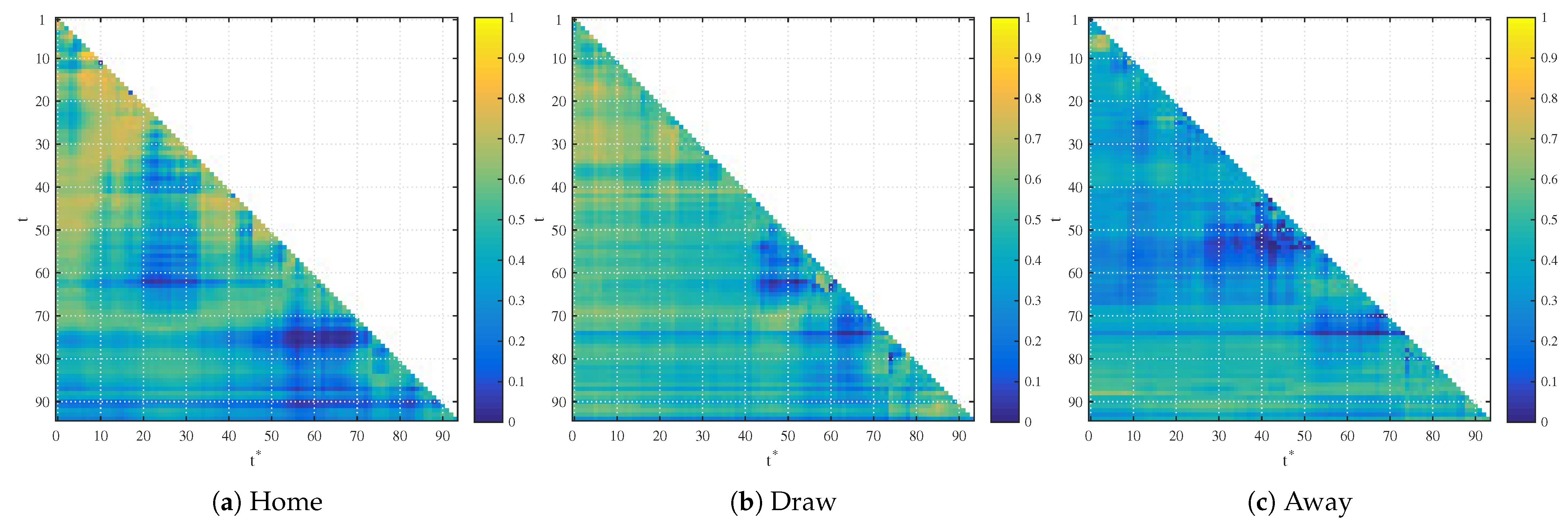
Figure 6 and Figure 7 show the results of trading in our studied market between the probability measure obtained from regression analysis and the market quote. The resulting value can be interpreted as a posterior probability that the measure obtained from regression analysis is correct as opposed to the market measure, giving a value between zero and one. The market interpretation of this result is that the agent’s resulting wealth represents a fraction of the total wealth of the market.
5. Conclusions
This paper’s main result is a link between the profit statistics of an agent maximizing logarithmic utility function and the traditional test statistics in terms of a likelihood ratio and Bayes factors. We illustrated this approach on prediction markets using the available football betting data. We constructed an alternative probabilistic estimate based on a regression analysis involving one current and one past market quote. In efficient markets, the current market quote should be already statistically unbeatable. The numerical analysis of the particular betting market did not reveal any substantially significant opportunities to beat the market.
Author Contributions
M.R. data analysis, model validation and implementation; J.V. theory linking likelihood to profit statistics. All authors have read and agreed to the published version of the manuscript.
Funding
This research was funded in part by Grant Agency of the Czech Republic grant number 18-01137S.
Institutional Review Board Statement
Not applicable.
Informed Consent Statement
Not applicable.
Data Availability Statement
3rd Party Data. Restrictions apply to the availability of these data. Data was obtained from Betfair and are available from the authors with the permission of Betfair.
Conflicts of Interest
The author declare no conflict of interest.
References
- Bernoulli, Daniel. 1954. Exposition of a new theory on the measurement of risk. Econometrica 22: 23–36. [Google Scholar] [CrossRef] [Green Version]
- Brown, Alasdair, J. James Reade, and Leighton Vaughan Williams. 2019. When are prediction market prices most informative? International Journal of Forecasting 35: 420–28. [Google Scholar] [CrossRef] [Green Version]
- Chen, Luyang, Markus Pelger, and Jason Zhu. 2019. Deep learning in asset pricing. arXiv arXiv:1904.00745. [Google Scholar]
- Croxson, Karen, and J. James Reade. 2014. Information and efficiency: Goal arrival in soccer betting. The Economic Journal 124: 62–91. [Google Scholar] [CrossRef]
- Fama, Eugene F. 1970. Efficient capital markets: A review of theory and empirical work. The Journal of Finance 25: 383–417. [Google Scholar] [CrossRef]
- Gil, Ricard, and Steven Levitt. 2007. Testing the efficiency of markets in the 2002 world cup. Journal of Prediction Markets 1: 255–70. [Google Scholar]
- Golec, Joseph, and Maurry Tamarkin. 1991. The degree of inefficiency in the football betting market: Statistical tests. Journal of Financial Economics 30: 311–23. [Google Scholar] [CrossRef]
- Graefe, Andreas, J Armstrong, Randall J. Jones, and Alfred Cuzan. 2014. Combining forecasts: An application to elections. International Journal of Forecasting 30: 43–54. [Google Scholar] [CrossRef]
- Gray, Philip, and Stephen Gray. 1997. Testing market efficiency: Evidence from the nfl sports betting market. Journal of Finance 52: 1725–37. [Google Scholar] [CrossRef]
- Horn, Christian, Michael Ohneberg, Bjoern Ivens, and Alexander Brem. 2014. Prediction markets—A literature review 2014 following tziralis and tatsiopoulos. Journal of Prediction Markets 8: 89–126. [Google Scholar] [CrossRef]
- Huberty, Mark. 2015. Can we vote with our tweet? on the perennial difficulty of election forecasting with social media. International Journal of Forecasting 31: 992–1007. [Google Scholar] [CrossRef]
- Jeffreys, Harold. 1935. Some tests of significance, treated by the theory of probability. In Mathematical Proceedings of the Cambridge Philosophical Society. Cambridge: Cambridge University Press, vol. 31, pp. 203–22. [Google Scholar]
- Kass, Robert E, and Adrian E Raftery. 1995. Bayes factors. Journal of the American Statistical Association 90: 773–95. [Google Scholar] [CrossRef]
- Kelly, John L. 1956. A New Interpretation of Information Rate. Bell System Technical Journal 35: 917–26. [Google Scholar] [CrossRef]
- Leigh, Andrew, and Justin Wolfers. 2006. Competing approaches to forecasting elections: Economic models, opinion polling and prediction markets. The Economic Record 82: 325–40. [Google Scholar] [CrossRef] [Green Version]
- LeRoy, Stephen. 1989. Efficient capital markets and martingales. Journal of Economic Literature 27: 1583–621. [Google Scholar]
- Neyman, Jerzy, and Egon Sharpe Pearson. 1933. Ix. on the problem of the most efficient tests of statistical hypotheses. Philosophical Transactions of the Royal Society of London. Series A, Containing Papers of a Mathematical or Physical Character 231: 289–337. [Google Scholar]
- Page, Lionel. 2012. It ain’t over till it’s over. Yogi Berra bias on prediction markets. Applied Economics 44: 81–92. [Google Scholar] [CrossRef]
- Page, Lionel, and Robert T. Clemen. 2013. Do prediction markets produce well-calibrated probability forecasts? The Economic Journal 123: 491–513. [Google Scholar] [CrossRef] [Green Version]
- Rothschild, David. 2015. Combining forecasts for elections: Accurate, relevant, and timely. International Journal of Forecasting 31: 952–64. [Google Scholar] [CrossRef]
- Sjoeberg, Lennart. 2009. Are all crowds equally wise? A comparison of political election forecasts by experts and the public. Journal of Forecasting 28: 1–18. [Google Scholar] [CrossRef]
- Vaughan Williams, Leighton. 2005. Information Efficiency in Financial and Betting Markets. Cambridge: Cambridge University Press. [Google Scholar]
- Vaughan Williams, Leighton, and J. James Reade. 2016. Forecasting elections. Journal of Forecasting 35: 308–28. [Google Scholar] [CrossRef] [Green Version]
- Vecer, Jan. 2020. Optimal Distributional Trading Gain: Generalizations of Merton’s Portfolio Problem with Implications to Bayesian Statistics. Available online: https://ssrn.com/abstract=3616661 (accessed on 18 August 2020).
- Vecer, Jan, Frantisek Kopriva, and Tomoyuki Ichiba. 2009. Estimating the effect of the red card in soccer: When to commit an offense in exchange for preventing a goal opportunity. Journal of Quantitative Analysis in Sports 5: 1–20. [Google Scholar] [CrossRef] [Green Version]
- Wang, Wei, David Rothschild, Sharad Goel, and Andrew Gelman. 2015. Forecasting elections with non-representative polls. International Journal of Forecasting 31: 980–91. [Google Scholar] [CrossRef] [Green Version]
- Wolfers, Justin, and Eric Zitzewitz. 2006. Interpreting Prediction Market Prices as Probabilities. Working Paper 12200. Cambridge: National Bureau of Economic Research. [Google Scholar]
Figure 1.
p-values of the second regression coefficient in home, draw and away betting markets.

Figure 2.
p-values of the second regression coefficient in home, draw and away betting markets.

Figure 3.
Evolution of the optimal wealth (in blue) of the market taker in two situations. In the first situation in the left graph, the market taker is right, meaning that the correct probability of success is , but the market maker quotes probability . The wealth of the market taker becomes statistically significant rather quickly, exceeding the 95% significance level graphed in orange. The non-smooth evolution of the statistical significance level is due to the discrete nature of the binomial distribution. The second situation in the right graph shows the opposite situation when the market maker quotes the correct probability , but the market maker believes in the incorrect probability of . In this case, the wealth of the market taker quickly converges to zero.

Figure 4.
Realized profit for trading with the initial unit bankroll for the models based on time regression.
Figure 4.
Realized profit for trading with the initial unit bankroll for the models based on time regression.

Figure 5.
Realized profit for trading with the initial unit bankroll for the models based on spatial regression.
Figure 5.
Realized profit for trading with the initial unit bankroll for the models based on spatial regression.

Figure 6.
Bayesian model comparison in home, draw and away betting markets, time models.

Figure 7.
Bayesian model comparison in home, draw and away betting markets, spatial models.


Table 1.
The time martingale test results for the data representing the home win, the away win, and the draw. Number of p-values that indicate significant second regression coefficients at 5% and 1% levels and the relative frequency in the brackets.
Table 1.
The time martingale test results for the data representing the home win, the away win, and the draw. Number of p-values that indicate significant second regression coefficients at 5% and 1% levels and the relative frequency in the brackets.
| p-Value | Home Win | Draw | Away Win |
|---|---|---|---|
| 5%-level | 110 | 75 | 840 |
| (2.46%) | (1.68%) | (18.81%) | |
| 1%-level | 20 | 12 | 363 |
| (0.45%) | (0.27%) | (8.13%) |
Table 2.
Results of the spatial martingale test for the datasets home win, away win and draw. Number of p-values that indicate significant second regression coefficients at a level of 5% and 1% and the relative frequency in brackets.
Table 2.
Results of the spatial martingale test for the datasets home win, away win and draw. Number of p-values that indicate significant second regression coefficients at a level of 5% and 1% and the relative frequency in brackets.
| p-Value | Home Win | Draw | Away Win |
|---|---|---|---|
| 5%-level | 35 | 48 | 45 |
| (2.86%) | (4.64%) | (3.67%) | |
| 1%-level | 9 | 42 | 38 |
| (0.73%) | (4.06%) | (3.10%) |
Table 3.
Average profits together with standard deviation in brackets based on trading probabilities obtained from regression analysis against the market for testing data.
Table 3.
Average profits together with standard deviation in brackets based on trading probabilities obtained from regression analysis against the market for testing data.
| Market | All | 5.00% | 1.00% |
|---|---|---|---|
| Home (Time) | 0.9552 | 0.1384 | 0.1475 |
| (0.6759) | (0.1511) | (0.2101) | |
| Draw (Time) | 0.9760 | 0.3006 | 0.2049 |
| (0.4158) | (0.3219) | (0.1995) | |
| Away (Time) | 0.6206 | 0.3132 | 0.2339 |
| (0.2883) | (0.1935) | (0.2081) | |
| Home (Spatial) | 1.6310 | 1.4482 | 0.8393 |
| (0.8059) | (0.9961) | (0.1702) | |
| Draw (Spatial) | 1.3450 | 1.1380 | 1.1739 |
| (0.5401) | (0.1709) | (0.1073) | |
| Away (Spatial) | 0.9578 | 1.1106 | 1.1508 |
| (0.2710) | (0.1556) | (0.0373) |
Publisher’s Note: MDPI stays neutral with regard to jurisdictional claims in published maps and institutional affiliations. |
© 2021 by the authors. Licensee MDPI, Basel, Switzerland. This article is an open access article distributed under the terms and conditions of the Creative Commons Attribution (CC BY) license (http://creativecommons.org/licenses/by/4.0/).
Share and Cite
MDPI and ACS Style
Richard, M.; Vecer, J. Efficiency Testing of Prediction Markets: Martingale Approach, Likelihood Ratio and Bayes Factor Analysis. Risks 2021, 9, 31. https://0-doi-org.brum.beds.ac.uk/10.3390/risks9020031
AMA Style
Richard M, Vecer J. Efficiency Testing of Prediction Markets: Martingale Approach, Likelihood Ratio and Bayes Factor Analysis. Risks. 2021; 9(2):31. https://0-doi-org.brum.beds.ac.uk/10.3390/risks9020031
Chicago/Turabian StyleRichard, Mark, and Jan Vecer. 2021. "Efficiency Testing of Prediction Markets: Martingale Approach, Likelihood Ratio and Bayes Factor Analysis" Risks 9, no. 2: 31. https://0-doi-org.brum.beds.ac.uk/10.3390/risks9020031
Note that from the first issue of 2016, this journal uses article numbers instead of page numbers. See further details here.