
A Machine Learning Approach for Micro-Credit Scoring


1
Department of Mathematics, College of Engineering, Design and Physical Sciences, Brunel University London, Uxbridge UB8 3PH, UK
2
Boston University, Boston, MA 02215, USA
3
African Institute for Mathematical Sciences (AIMS), Kigali P.O. Box 7150, Rwanda
4
Department of Mathematical Sciences, Institute for Financial and Actuarial Mathematics, University of Liverpool, Liverpool L69 3BX, UK
*
Author to whom correspondence should be addressed.
†
These authors contributed equally to this work.
Risks 2021, 9(3), 50; https://0-doi-org.brum.beds.ac.uk/10.3390/risks9030050
Submission received: 18 February 2021
/
Revised: 28 February 2021
/
Accepted: 1 March 2021
/
Published: 9 March 2021
(This article belongs to the Special Issue Interplay between Financial and Actuarial Mathematics)
Abstract
:In micro-lending markets, lack of recorded credit history is a significant impediment to assessing individual borrowers’ creditworthiness and therefore deciding fair interest rates. This research compares various machine learning algorithms on real micro-lending data to test their efficacy at classifying borrowers into various credit categories. We demonstrate that off-the-shelf multi-class classifiers such as random forest algorithms can perform this task very well, using readily available data about customers (such as age, occupation, and location). This presents inexpensive and reliable means to micro-lending institutions around the developing world with which to assess creditworthiness in the absence of credit history or central credit databases.
1. Introduction
During the last few decades, credit quality emerged as an essential indicator for banks’ lending decisions (Thomas et al. 2017). Numerous elements reflect the borrower’s creditworthiness, and the use of credit scoring mechanisms could moderate the estimation of the probability of default (PD) while predicting the individual’s payment performance. The existing literature concentrates on understanding why organizations’ lending mechanisms are successful at decreasing defaults or addressing the issues from an economic theory perspective; see, e.g., Brau and Woller (2004); Jarrow and Protter (2019). More specifically, Demirgüç-Kunt et al. (2020) reported that almost one-third of the world’s adult population were unbanked, according to a 2017 world bank report. Therefore, they rely on micro-finance institutions’ services. Jarrow and Protter (2019) acknowledged the gap in the existing literature on how to determine fair lending rates in micro-finance, which would be granting lending access (or credit) to low-income populations excluded from traditional financial services.
Credit scoring refers to the process of evaluating an individual’s creditworthiness that reflects the level of credit risk and determines whether an application of the individual should be approved or declined (Thomas et al. 2017). Financial lending services assess credit risk by employing decision models and techniques. These institutions assess the level of risk required to meet their financial obligations (Zhao et al. 2015). Credit scoring is essential in a micro-lending context, although a lack of credit history and sometimes even a bank account requires innovative ways to assess an individual’s creditworthiness. Financial institutions and non-bank lenders who regularly provide credit information on their customers’ accounts to the credit bureau can obtain credit information reports from the bureau to appraise new loan applications’ creditworthiness and examine accounts on pay-per-use fees and a membership fee. However, the statutory framework for credit reporting access data varies from country to country. Thus, depending on the jurisdiction, borrower permission might be required to provide data to the bureau and access a credit report (IFC 2006). However, for unbanked customers, such a centralized record of past credit history is often missing. A growing group of quantitative and qualitative techniques has been developed to model these credit management decisions in determining micro-lending scoring rates by considering various credit elements and macroeconomic indicators. Early studies have attempted to address the issue mainly by employing linear or logistic regression (Provenzano et al. 2020). While such models are commonly fitted to generate reasonably accurate estimation, these early era techniques have been succeeded by machine learning techniques that have been extensively applied in various scientific disciplines, for example, medicine, biochemistry, meteorology, economics, and hospitality. For example, Ampountolas and Legg (2021); Aybar-Ruiz et al. (2016); Bajari et al. (2015); Barboza et al. (2017); Carbo-Valverde et al. (2020); Cramer et al. (2017); Fernández-Delgado et al. (2014); Hutter et al. (2019); Kang et al. (2015); Zhao et al. (2017) have reported applications of machine learning in a variety of fields and achieved staggering results. In credit scoring, in particular, Provenzano et al. (2020) reported good estimation results using machine learning.
Similarly, numerous studies on the applicability of machine learning techniques have been implemented in other areas of finance due to their ability to recognize a set of financial data trends; see, e.g., Carbo-Valverde et al. (2020); Hanafy and Ming (2021). Related studies indicated that a combination of machine learning methods could offer high credit scores accuracy; see, e.g., Petropoulos et al. (2019); Zhao et al. (2015). Nowadays, credit risk assessment has become a rather typical practice for financial institutions, with decisions generally received based on the borrowers’ credit history. However, the situation is rather different for institutions providing micro-finance services (micro-finance institutions—MFIs).
The novelty in this research is a classifier that indicates the creditworthiness of a new customer for a micro-lending organization. For such organizations, third-party information on consumer creditworthiness is often unavailable. We propose to evaluate credit risk using a combination of machine and deep learning classifiers. Using real data, we compared the accuracy and specificity of various machine learning algorithms and demonstrated these algorithms’ efficacy in successfully classifying customers into various risk classes. This is the first empirical study to examine the use of machine learning for credit scoring in micro-lending organizations in the academic literature to the best of the authors’ knowledge.
In this assessment, we have compared seven machine and deep learning models to quantify the models’ estimation accuracy when measuring individuals’ credit scores. In our experiments, ensemble classifiers (XGBoost, Adaboost, and random forest) exhibited better classification performance in terms of accuracy, about 80%, whereas the popular multilayer perceptron model yielded about 70% accuracy. We tuned the classifier’s hyperparameters to obtain the best possible decision boundaries for better institutional micro-lending assessment decisions for all the classifiers. While these experiments were for a single dataset, they point to micro-lending institutions’ choices in terms of off-the-shelf machine learning algorithms for assessing the creditworthiness of micro-loan applicants.
This research is organized as follows: Section 2 provides an overview of prior literature on each machine learning technique we employ to evaluate credit scoring. Even though these techniques are standard, we provide an overview here for completeness of discussion. In Section 3, we introduce the research methodology and data evaluation. Section 4 presents the analytic results of the various machine learning techniques, and in Section 5, we discuss the results. Finally, Section 6 contains the research conclusions.
2. Literature Review
2.1. Machine Learning Techniques for Consumer Credit Risk
Khandani et al. (2010) have employed machine learning techniques to build nonlinear non-parametric forecasting approaches to measure consumer credit risk. To identify credit cardholders’ defaults, the authors used a credit office data set and commercial bank-customer transactions to establish a forecast estimation. Their results indicate cost savings from 6% to 25% of total losses when machine learning forecasting techniques are employed to estimate the delinquency rates. Besides, their study opens up questions of whether aggregated customer credit risk analytics may improve systematic risk estimation.
Yap et al. (2011) used historical payment data from a recreational club and established credit scoring techniques to identify potential club member subscription defaulters. The study results demonstrated that no model outperforms the others among a credit scorecard model, logistic regression, and a decision tree model. Each model generated almost identical accuracy figures.
Zhao et al. (2015) examined a multi-layer perceptron (MLP) neural network’s accuracy regarding estimating credit scores efficiently. The authors used a German credit dataset to train and estimate the model’s accuracy. Their results indicated an MLP model containing nine hidden units achieved a classification accuracy of 87%, higher than other similar experiments. Their study results proved the trend of MLP models’ scoring accuracy by increasing the number of hidden units.
In Addo et al. (2018) the authors examined credit risk scoring by employing various machine and deep learning techniques. The authors used binary classifiers in modeling loan default probability (DP) estimations by incorporating ten key features to test the classifiers’ stability by evaluating performance on separate data. Their results indicated that the models such as the logistic regression, random forest, and gradient boosting modeling generated more accurate results than the models based on the neural network approach incorporating various technicalities.
Petropoulos et al. (2019) studied a dataset of loan-level data of the Greek economy of examining credit quality performance and quantification of probability default for an evaluating period of 10 years. The authors used an extended example of classifications of the incorporated machine learning models against traditional methods, such as logistic regression. Their results identified that machine learning models had demonstrated superior performance and forecasting accuracy through the financial credit rating cycle.
Provenzano et al. (2020) introduced machine learning models to compose credit rating and default prediction estimation. They used financial instruments, such as historical balance sheets, bankruptcy statutes, and macroeconomic variables of a Moody’s dataset. Using machine learning models, the authors observed excellent out-of-sample performance results to reduce the bankruptcy probability or improve credit rating.
2.2. Machine Learning Algorithms
Machine learning-based systems are growing in popularity in research applications in most disciplines. Considerable decision-making knowledge from data has been acquired in the broad area of machine learning, in which decision-making tree-based ensemble techniques are recognized for supervised classification problems. Thus, classification is an essential form of data analysis in data mining that formulates models while describing significant data classes (Rastogi and Shim 2000). Accordingly, such models estimate categorical class labels, which can provide users with an enhanced understanding of the data at large Han et al. (2012) resulted in significant advancements in classification accuracy.
Motivated by the preceding literature, we evaluated a large number of machine learning algorithms in our work on credit risk in micro-lending. A set of algorithms that performed well in numerical experiments with real data is explained in more details below.
2.2.1. AdaBoost
Adaptive boosting (AdaBoost) is an ensemble algorithm incorporated by Freund and Schapire (1997), which trains and deploys trees in time series; see Devi et al. (2020) for discussion in details. Since then, it evolved as a popular boosting technique introduced in various research disciplines. It merges a set of weak classifiers to build and boost a robust classifier that will improve the decision tree’s performance and improve accuracy (Schapire 2013).
The mathematical presentation of the AdaBoost classifier at a high level is described of the following (see Schapire et al. (2013) for more details):
Consider that training data ( and ), …, ( and ) are the ∈X, ∈ {−1, +1}.
Then the parameters of AdaBoost classifier are initialized: = 1/m for i = 1, …, m. For t = 1, …, T:
- Train weak learner using distribution .
- Attain weak hypothesis : X⟶ {−1, +1}.
- Aim: select with low weighted error:
Select = ln.
Hence, for :
where is a normalization factor (chosen so that will be a distribution).
Which generates an output of the final hypothesis as following:
Therefore, H is estimated as a weighted majority vote of the weak hypotheses while assigning each hypothesis a weight (Schapire et al. 2013).
2.2.2. XGBoost
XGBoost (extreme gradient boosting method) was proposed in Chen and Guestrin (2016). It is a gradient algorithm based on scalable tree boosting that manages parallel processing. Tree boosting represents an effective and extensively employed machine learning method. The boosted trees are formed to address regression and classification trees’ flexibly while optimizing the outcome’s predictive state. Furthermore, gradient boosting adjusts the boosted trees by capturing the feature scores and promoting their weights to the training model when employed with historical data. More details about this algorithm may be found in Friedman et al. (2001) and Hastie et al. (2009).
To advance model generalization with XGBoost, Chen and Guestrin suggested an adjustment to the cost function, making it a “regularized boosting” technique:
with,
where indicates classification’s tree number of leaves , and w is the value associated with each leaf. The regularizer corrects the model’s complexity and can be decoded as the ridge regularization of coefficient and Lasso regularization of coefficient . Besides, L is a differentiable convex loss function that estimates the difference between the prediction , and the target , where is the i prediction of the i-th instance. Thus, when the parameter is fixed to zero, the cost function befalls backward to the classical gradient tree boosting; see, e.g., Abou Omar (2018).
The algorithm starts from a single leaf, and weights the importance of “frequency”, “cover”, and “gain” in each feature, and accumulates branches on the tree. Frequency signifies the relative number of times a feature occurs; for example, higher frequency scores imply continuing employment of a feature in the boosting process. The cover represents the number of observations associated with the specific feature. Finally, gain indicates the primary contributing factor to each constructed tree. Hence, to estimate the standardized objective, each leaf consists of adding first and second-order derivatives, which boosts its decline when examining for splits (Friedman et al. 2001).
where and . By excluding the constant term, we obtain an approximation of the objective at step t as following:
By defining as the instance set at leaf j and expanding , we can rewrite the equation as:
XGBoost applies the following gain instead of using entropy or information gain for splits in a decision tree:
where the first term is the score of the left child; the second is the score of the right child, if we do not split the third the score; is the complexity cost if we add a new split (Abou Omar 2018; Friedman et al. 2001).
2.2.3. Decision Tree Classifier
Decision tree classifiers have been widely implemented in numerous distinct areas. The tree flow display is comparable to a progress diagram, with a tree structure in which cases are arranged based on their feature values (Szczerbicki 2001). Thus, a tree may be a leaf associated with one class. Decision tree classifiers’ significant feature refer to obtaining detailed decision-making experience based on the data set utilized (Panigrahi and Borah 2018). The process for generating such a decision tree is based around the training set of objects S, and each being affiliated with one of the classes , , …, (Quinlan 1990). Hence, (a) if all the objects in S associate with an equal class, for instance, , the decision tree for S comprises a leaf identified with this class, and (b) apart from that, let T be any test with expected results . Thus, each object in S possess one result for T, so the test distributes S into subsets , in which each object in has result for T. Therefore, for each outcome —T is a decision’s tree root—we establish a secondary decision tree by requesting a similar process recurring on the set (Quinlan 1990).
2.2.4. Extra Trees Classifier
The extremely randomized trees classifier (extra trees classifier) establishes an ensemble of decision trees following an original top-down approach (Geurts et al. 2006). Thus, it is similar to a random forest classifier differing only in the decision trees’ mode of construction. Each decision tree is formed from the initial training data set sample. It entails random both element and cut-point choice while dividing a node of a tree. Hence, it differs from other tree-based ensemble approaches because it divides nodes by determining cut-points entirely at random, and it practices on the entire training sample to grow the trees (Ampomah et al. 2020). The practice of using the entire initial training samples instead of bootstrap replicas is to decrease bias. At each test node, each extra trees algorithm is provided by the number of decision trees in the ensemble (denote by M), the number of features randomly selected at each node (K), and the minimum number of instances needed to split a node () (Geurts et al. 2006). Hence, each decision tree must choose the best feature to split the data based on some criteria, leading to the final prediction by forming multiple decision trees (Acosta et al. 2020).
2.2.5. Random Forest Classifier
The random forest classifier is an ensemble method algorithm of decision trees wherein each tree depends on randomly selected samples trained independently, with a similar distribution for all the trees in the forest (Breiman 2001). Hence, a random forest is a classifier incorporating a collection of tree-structured classifiers that decrease overfitting, resulting in an increase in the overall accuracy (Geurts et al. 2006). As such, random forest’s accuracy differs based on the strength of each tree classifier and their dependencies.
where . We can achieve the estimate of with respect to the parameter by taking the expectation of (Addo et al. 2018).
2.2.6. K-Nearest Neighbors Classifier
K-nearest neighbors (k-NN) is one of the oldest machine-learning non-parametric techniques, which makes it one of the most popular approaches used to form classification (Fix 1951; Fix and Hodges 1952). Conceptually, we use a large volume of training data, where a set of variables characterizes each data point. The algorithm assumes that similar things exist nearby, the k-nearest neighbors; hence, the k-NN algorithm is employed to rapidly search the space and find the similar maximum items, based on a square root of N approach, for the total volume of points in the training data set. For example, assuming a point we wish to classify into one of k groups, we can identify k observed data points nearest to . The classification form assigns to the sample that employs the most observed data points out of the k-nearest neighbors (Neath et al. 2010). To that end, the similarity depends on a particular distance metric; thus, the classifier’s efficiency depends considerably on the distance metric incorporated (Weinberger and Saul 2009). Finally, it is based on two independent processes with the adjacency matrix to be first constructed following by estimating the edge’s weights (Dornaika et al. 2017).
2.2.7. Neural Network
Artificial neural networks (ANN) represent an important class of non-linear models. The growth of computational intelligence has been successfully applied to the development of ANN model forecasting applications for prediction of demand (Zhang et al. 1998). An empirical application of ANNs has demonstrated satisfactory forecasting performance with evidence mainly published in many industries. Therefore, different ANN models have been popular in the forecasting literature, with several examples coming from electricity forecasting, but also from forecasting financial data.
2.2.8. Multilayer Perceptron Model
This subsection and the rest of the paper will focus on the most common ANN-type model; a feed-forward neural network—the multilayer perceptrons (MLP). The MLP networks each contain a set of inputs () and three or more layers of neurons with nonlinear activation functions; they are being used in all sorts of problems, particularly in forecasting because of their fundamental ability of arbitrary input–output mapping (Zhang et al. 1998):
where is the output vector at time t; I refers to the number inputs , which can be lags of the time series; and H indicates the number of hidden nodes in the network. The weights , with and are for the hidden and output layers, respectively. Similarly, the and are the biases of each node, while is the transfer function, which might be either the sigmoid logistic or the tanh activation function.
3. Methodology
3.1. Data Collection
The data used in this paper were obtained from Innovative Microfinance Limited (IML), a micro-lending institution in Ghana. It started operating in 2009. The data are an extract of information that IML could make available to us on micro-loans from January 2012 to July 2018, during a period of economic and political stability. During this period, the market’s liquidity risk was the most significant risk (Johnson and Victor 2013). A total sample size of 4450 customers was extracted, but 46 rows were entirely deleted due to many missing values in those rows. The data fundamentally consist of customer information, such as demographic information, amount of money borrowed, frequency of loan repayment (weekly or monthly), outstanding loan balance, number of repayments and number of days in arrears. To reduce the level of variability in the loan amount, we took the logarithm of it and named the new variable “log amount”. Additionally, given the fact that the micro-loans have different periods of repayment and frequency of repayment, all interest rates were annualized to take care of these differences by bringing them to a common denominator in terms of time.
Table 1 below is a list of the variables used in this paper to fit our classification models.
3.2. Definitions of Risk Classes
In this paper, we consider three risk classes for the multi-class classification problem. A risk is considered “good” if the customer is not in arrears or is in arrears for less than 30 days; it is considered “average” if the customer is in arrears between 30 and 91 days; finally, it is considered “poor if the customer is in arrears for more than 91 days.
3.3. Data Balancing
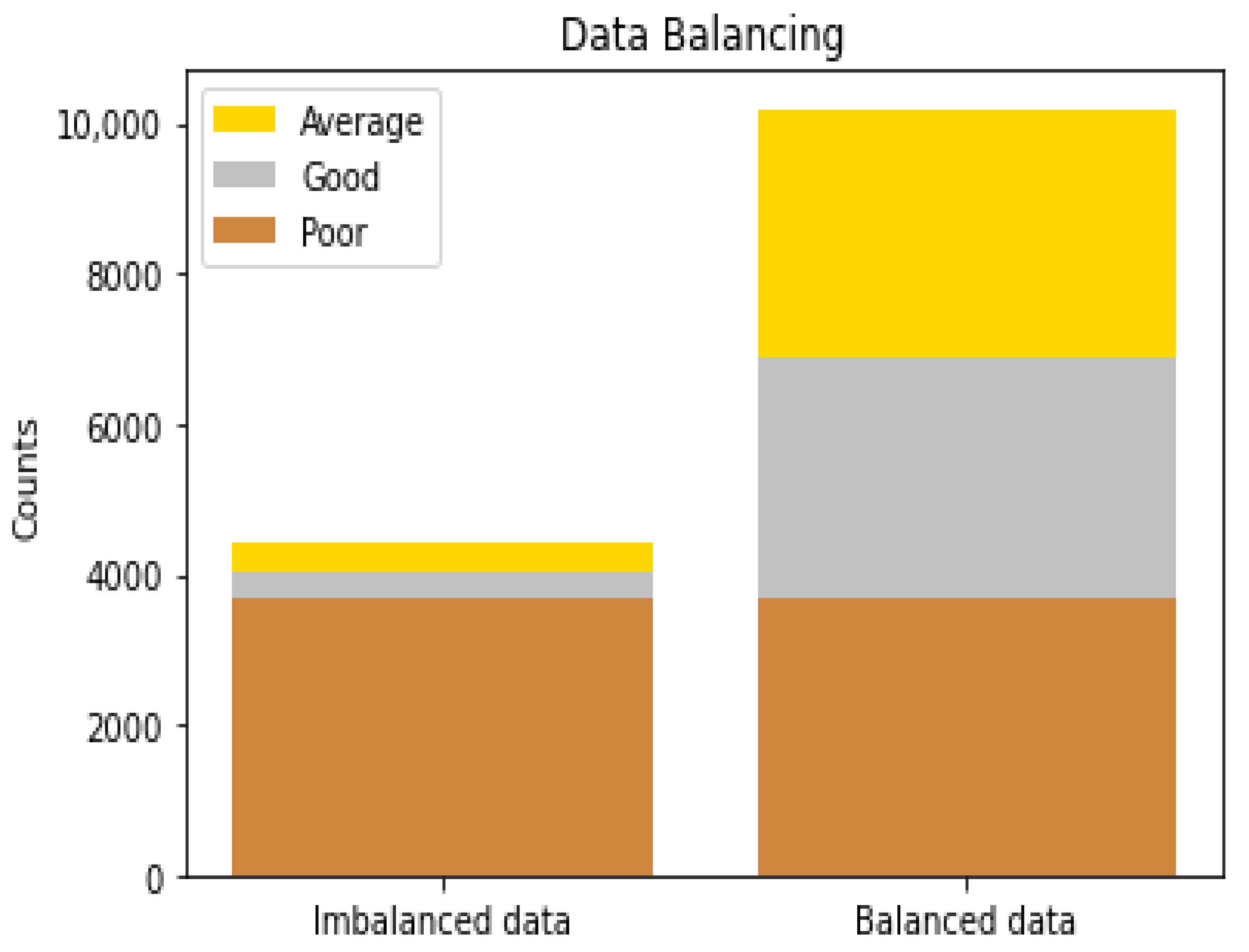
After classifying all customers into the various risk classes, we encountered an imbalance data situation wherein 83.72% of the entire data set belonged to the poor risk class. In such a case, the danger is that any model fitted to the data might end up predicting the majority risk class all the time, even though the model diagnostics show that the model is good. To address this class imbalance condition, we adopted the machine learning synthetic minority over-sampling technique for nominal and continuous (SMOTENC for short) to over-sample the minority classes to achieve fair representation for all classes in the data set. After this, the majority class constituted only 36.19% of the data set. Figure 1 shows the nature of the data set before and after applying the SMOTENC algorithm:
3.4. Training–Test Set Split
For all the models fitted in this study, we split the balanced data into 80% for the training set and 20% for the testing set (validation). Unless otherwise stated, all analyses presented in this paper were done using the Python programming language.
3.5. Summary Statistics of Features
Table 2 presents the summary statistics of the numerical features used in this paper. A second quartile (median) value of 31 for age implies that 50% of customers are 31 years old or younger, while the remaining 50% are more than 31 years old. Meanwhile, 25% of customers are 26 (first quartile) years old or younger, and about 75% are 58 years old (third quartile) or younger. A positive skewness for age means that most customers are below the mean age. This also explains why the median age is lower than the mean age. Additionally, a negative excess kurtosis implies that age distribution is platykurtic in nature (i.e., it has a flat top, a plateau). Thus, the distribution is less peaked than that of the Gaussian distribution. The explanations given for the descriptive statistics of age can be transferred (in a parallel sense) to explain that of the remaining features.
Note that even though annualized rate is positively skewed, the original interest rates (i.e., before they were annualized) have negative skewness, which means most customers pay an interest rate higher than the mean value. However, this conclusion could be biased, given that the micro-loans have varying durations and frequencies of payment. Hence, this paper adopted annualized rate. Loan amount had a standard deviation of 4169.1886, which negatively influenced the classifiers, most likely due to the wide dispersion. Therefore in this paper, log amount was used instead.
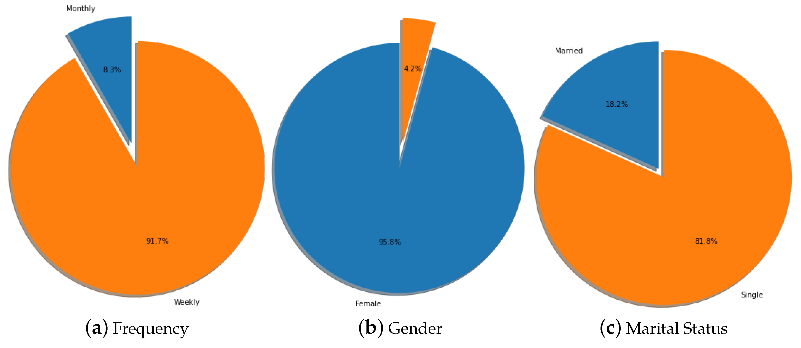
For the categorical features, we used each category’s proportions to describe them as shown in Figure 2 below.
In Figure 2 above, gender is the most disproportionate feature, with the majority being women. This is not surprising because previous studies have shown that about 75% of micro-credit clients worldwide are women and have proven to have higher repayment rates, and will usually accept micro-credit more easily than men (Chikalipah 2018). For example, Grameen Bank currently has 96.77% of its customers being women due to the extensive micro-credit services it offers (Grameen Bank 2020).
3.6. Feature Selection
The dataset had more variables than those used in this paper. Some of the variables were of no use to us, such as customer ID which is simply a unique customer identifier for all customers in the data. Other variables, such as date of birth, date disbursed, and date due were not used. However, we did calculate the age feature from the date of birth and date disburse by finding the difference in days between the date on which the loan was issued to each customer and birth date. The number of days was then divided by days to obtain the age in years at the time of issuing the micro-loan. The choice of days was to capture leap year effects in the age calculations. Additionally, note that to obtain the age at which a customer joined the scheme, the curtated age (i.e., the whole number part of the age) was considered; the fractional (i.e., decimal) part of the age was ignored. We chose to use the customers’ personal information, which included age, gender, and marital status, as our first choice of features.
Outstanding loan balance was not used because for a new customer the outstanding loan balance is the same as the loan amount. Moreover, there is a high positive linear correlation of 0.97 between these two variables. Eliminating one of them from the model helped to remove the confounding effect from the models. This confounding effect is a result of the presence of multicollinearity between these features. In such a situation, one of the features becomes redundant. Eliminating one such feature from the models helps prevent them from overfitting or underfitting, which avoids the case where a small change in the data leads to a drastic effect on the model in question. Some authors hold the notion that the multicollinearity effect is tamed in machine learning models, but it still has some effect on the models; besides, this notion is not widely accepted.
After this, frequency, interest rates, and number of repayments were then added to the set of features, since they were the only remaining variables that could be used as predictors. As explained earlier, log amount and annualized rate were used instead of amount and interest rate.
4. Results
In this section, we present analytic results of the various machine learning models adopted in this paper. All model diagnostic metrics in this paper are based on the validation/test set.
4.1. Prediction Accuracy
The idea here was to determine which model performs best with our data, and as a first step, we considered each model’s overall out-of-sample prediction accuracy on the test set. Note that as a rule of thumb, it is advisable to use the global f1-scores for model comparison instead of the accuracy metric; however, in our case, the two metrics were the same for all classifiers. The results are shown in the table below:
From Table 3, the least performing model in terms of prediction accuracy was the artificial neural network multilayer perceptron. Unlike the popular opinion held about neural network models in the literature, the predictive power did not improve irrespective of the number of hidden layers and/or hidden nodes. However, note that the best performing models were the machine learning ensemble classifiers (random forest, XGBoost, and Adaboost). XGBoost and Adaboost slightly outperformed the random forest classifier. Note that apart from the out-of-sample prediction accuracy on the validation set, other model diagnostic metrics such as confusion matrix, receiver operating characteristic (ROC) curve, area under the curve (AUC), f1-score, precsion, and recall showed that the ensemble classifiers performed better with our data set than the rest of the models. Therefore, for the rest of this paper, we concentrate our analyses on the ensemble classifiers.
4.2. Confusion Matrix
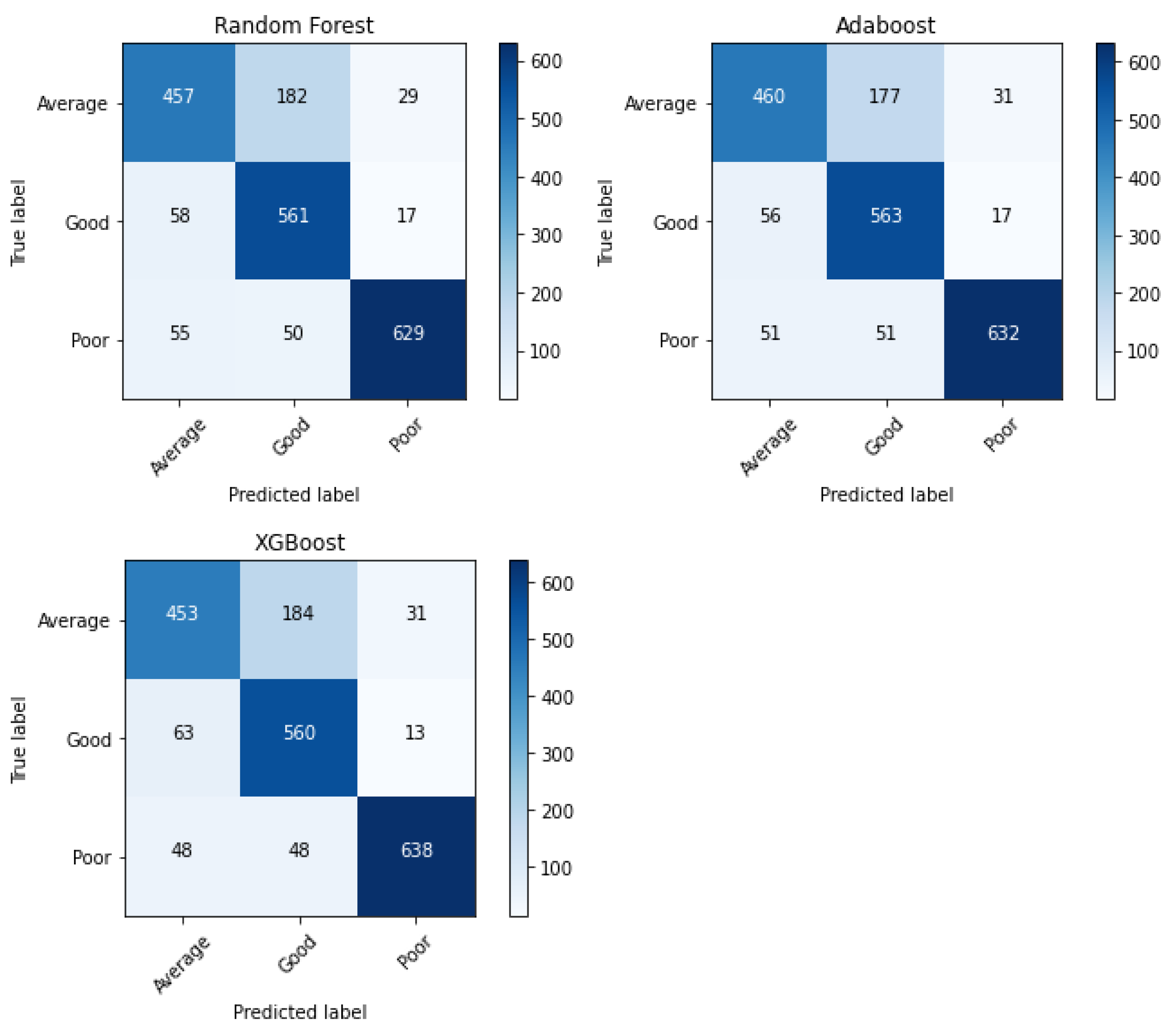
There is a need to look at the confusion matrix to assess a classification model’s quality of classification. For an ideal confusion matrix, we expect to get values only on the leading/principal diagonal, since they represent correct classification; values off-diagonal are those that were misclassified. Hence, Figure 3 illustrates the confusion matrix for each of our ensemble classifiers.
Figure 3 above shows that most of the values lie along the principal diagonal for all the ensemble classifiers, and the more values we record on the principal diagonal, the more evidence we have of correct classification. However, one thing that is easily noticeable is that most of the misclassifications are recorded between the average and good risk classes for all the classifiers. This is most likely because the decision boundary between the two classes is not so visible; hence, the classifiers cannot easily identify it, leading to some misclassifications between the two classes. However, for each classifier, the hyperparameters were tuned to obtain the best possible model that could quickly and easily identify the decision boundaries for a better classification experience.
4.3. Classification Report
In this subsection, we examine each classifier’s precision, recall, and f1-score.
Hence, Table 4 below presents the classification report for the XGBoost model. Note that precision is the ratio of predicted values of a risk class that actually belong to that class to all values. In any of the confusion matrices above, it is the ratio of the values on the leading diagonal to the sum of all values in that column. Recall (true positive rate), on the other hand, is a ratio of the actual values of a risk class that were actually predicted as belonging to that class. Precision and recall usually have inverse relations, and the f1-score is a metric that measures both precision and recall together; it presents a combined picture of both precision and recall. It is a harmonic mean of the two metrics. Support is the actual number of occurrences of a particular risk class in the data set (usually the validation data). The accuracy parameter is simply the overall predictive power of the classifier. It is simply the ratio of the sample data that the classification model correctly classified. In each of the confusion matrices above, the sum of all elements on the principal diagonal is divided by the sum of all elements in the confusion matrix to obtain each classifier’s accuracy. The micro-average metric is the arithmetic mean of the precision, recall, and f1-scores, while the weighted average computes the weighted average of the precision, recall, and f1-scores. Note that these two metrics (micro-average and weighted average) compute precision, recall, and f1-score globally for the classifier. Global support is the sum of the individual supports for each risk class. The explanation given above for the XGBoost classifier can be mirrored for the random forest and AdaBoost classifiers; therefore, we present the same metrics for the random forest and AdaBoost classifiers in Table 5 and Table 6 below. Note that the three ensemble classifiers have identical values for all the model diagnostic metrics.
4.4. Sensitivity Analysis
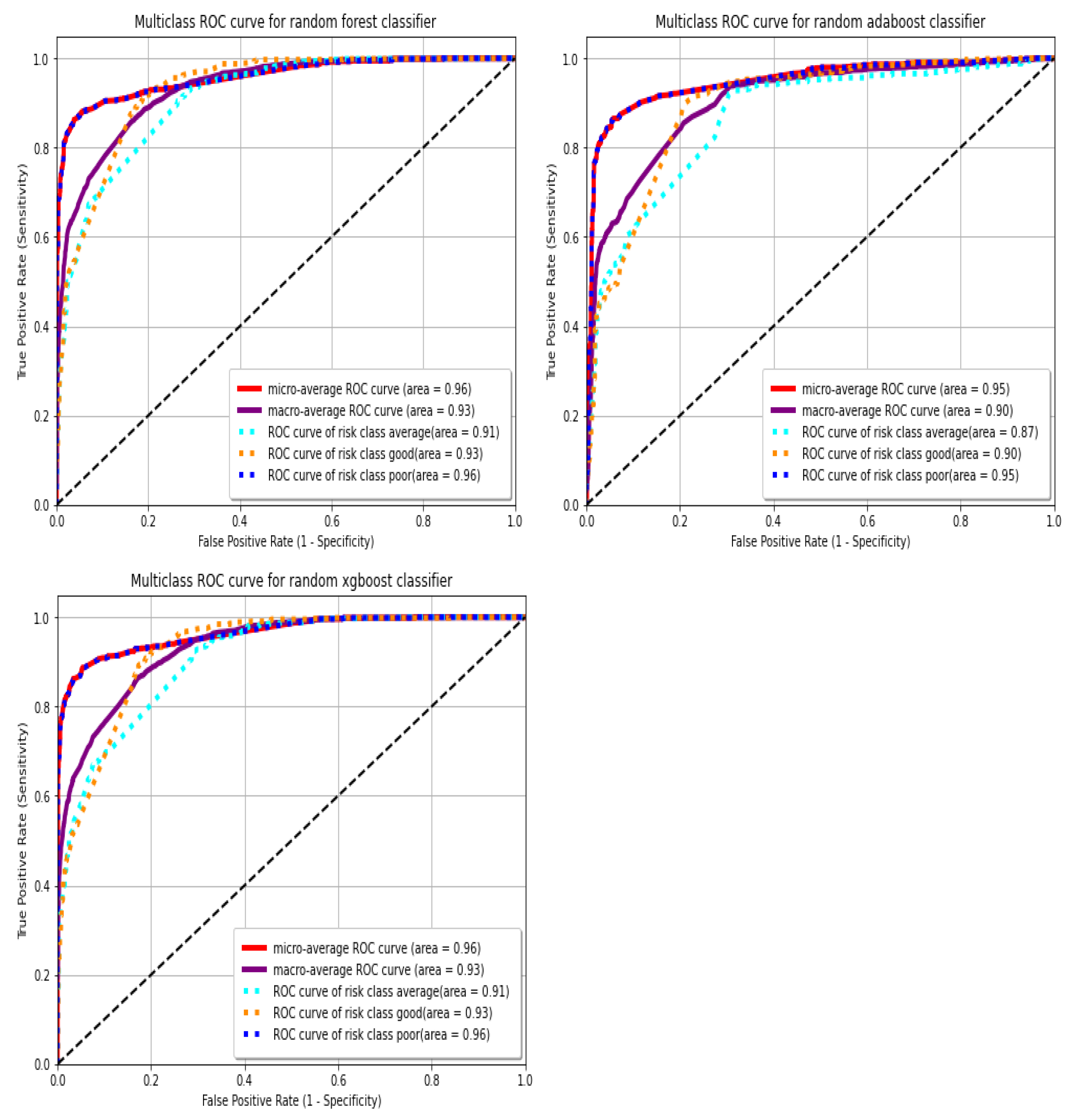
Here we present the receiver operating characteristic (ROC) curves and their respective areas under the curve (AUCs). ROC curves and AUCs are used to measure the quality of a classifier’s output; thus, they measure how correctly a classifier has been tuned. Movement along the ROC curve is typically a trade-off between the classifier’s sensitivity (true positive rate (TPR)) and specificity (TNR), and the steeper the curve, the better. For the ROC curve, sensitivity increases as we move up, and specificity decreases as we move right. The ROC curve along a 45 angle is as good a tossing a coin (i.e., a classifier as good as a random guess). Additionally, the closer the AUC is to 1, the better it is. Consider the figures below (Figure 4):
In Figure 4, for each classifier, we show the ROC curve and AUC for each risk class. ROC curves are typically for binary classification, but we used them pairwise for each class for multiclass classification. We adopted the one-versus-rest approach. This approach evaluates how best each classifier can predict a particular risk class against all other risk classes. Hence, we have an ROC curve and AUC for each class against the rest of the classes, and the unweighted averages of all these ROC curves and AUCs are the global (macro) ROC curve and AUC for that classifier; this means each risk class is treated with an equal weight of if there are k classes. The micro-average metric is a weighted average taking into effect the contribution of each risk class. It calculates a single performance metric instead of several performance metrics that are averaged in the case of a macro-averaged AUC. Mostly, in a multiclass classification problem, the micro-average is desired if there is a class imbalance situation (i.e., if the main concern is the overall performance on the data and not any particular risk class in question). In that case, the micro-average tends to bring the weighted average metric closer to the majority class metric. However, in this paper, the class imbalance problem was taken care of, even before fitting the classification models. The results for each classifier are shown in Figure 4 above. The ROC curves and AUCs for all the ensemble classifiers look quite good, as the ROC curves are high above the 45 line, and the AUCs are high above the 0.5 (random guess) threshold. This is an indication that our ensemble classifiers have good predictive power, far better than random guessing. Note that the ROC curves and AUCs presented for all the classifiers above are based on the validation/test set.
4.5. Feature Importance
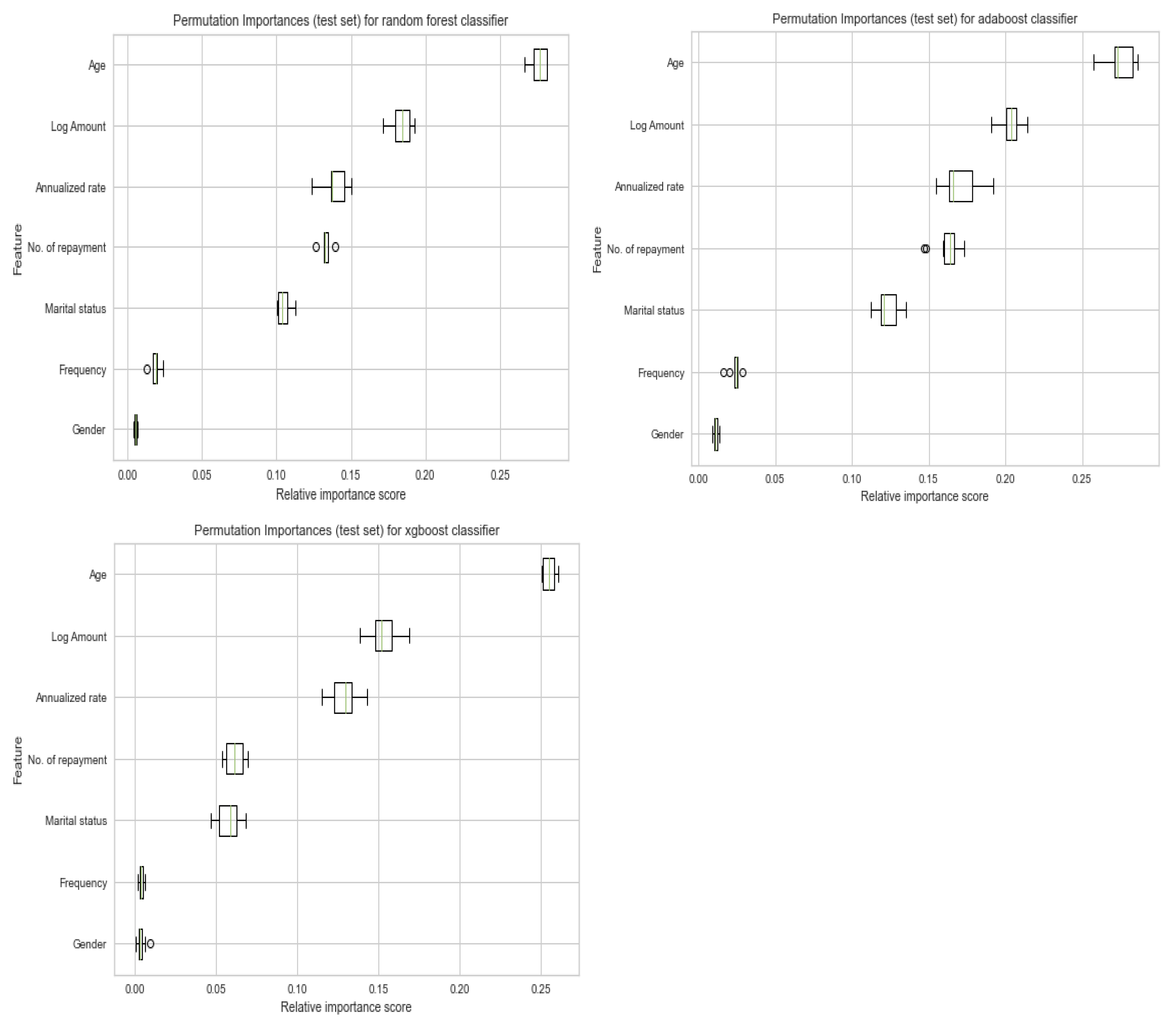
In this subsection, we evaluate the relative importance of each predictive variable in predicting default. Consider the Figure 5 below:
Figure 5 above adopted the permutation importance score (on the validation/test set) to evaluate our predictive features’ relative importance in predicting defaults on micro-loans. The choice of permutation importance score is due to its ability to overcome the impurity-based feature importance score’s significant drawbacks. As revealed in the Scikit Learn documentation, the impurity-based feature importance score suffers from two major drawbacks. First of all, it gives priority to features with many distinct elements (i.e., features with very high cardinality); hence, it favors numerical features at the expense of categorical features. Secondly, it is based on the training set. It, therefore, does not necessarily reflect a feature’s importance or contribution when making predictions on an out-of-sample data set (i.e., test set)—thus, the documentation states, “The importances can be high even for features that are not predictive of the target variable, as long as the model has the capacity to use them to overfit”.
For all our classifiers, the top three most important features in predicting default on micro-loans are age, log amount, and annualized rate. We also realized that numerical features have more relative importance in predicting default than categorical features for all the classifiers.
4.6. Tuning of Hyperparameters
In this subsection, we present the optimal hyperparameters obtained for each of the top three ensemble classifiers. Consider the Table 7 below:
Note that for all the classifiers, default values were used for any hyperparameters not listed in the table above. For all the classifiers, the hyperparameter “number of estimators” has proven to be very crucial in getting optimal accuracy. The hyperparameter “eta/learning rate” has also shown great importance in the XGBoost and AdaBoost classifiers. It is noticed that there is a trade-off between learning rate and number of estimators for the boosting classifiers (i.e., there is an inversely proportional relationship between them). Additionally, note that by keeping all other optimal parameters constant, model accuracy increases with an increasing number of estimators until it reaches the point of the optimal values reported in Table 7 above. Above this level, the accuracy starts to reduce such that if it were plotted, it would have a bell shape. This holds for the top three ensemble classifiers presented in this paper.
5. Discussion
This paper evaluated the usefulness of machine learning models in assessing defaulting in a micro-credit environment. In micro-credit, there is usually no central credit database of customers and very little to no information at all on a customer’s credit history; this situation is predominant in Africa, where we got our data from. This makes it hard for micro-lending institutions to determine whom to deny or not deny micro-loans. To overcome the drawback, this paper demonstrates that machine learning algorithms are powerful in extracting hidden information in the data set, which helps to assess defaults in micro-credit. All performance metrics adopted in this paper were those based on the validation/test set. The data imbalance situation in the original data set was solved using the SMOTENC algorithm. Several machine learning models were fitted to the data set, but this paper reported only those models that recorded overall accuracy of 70% or higher on the validation set. Most of the models reported in this paper are tree-based algorithms, possibly because we have many categorical features in our data set, and tree-based classifiers have been known to generally work better with such data sets than other machine learning algorithms that are not tree-based. Among the models reported in this paper, the top three best performing classifiers (random forest, XGBoost, and Adaboost) are all ensemble classifiers and tree-based algorithms as well. It might be the case that tree-based algorithms are powerful for predicting defaulting in a micro-credit environment. All ensemble classifiers reported an overall accuracy of at least 80% on the validation set. Other performance measures adopted also revealed that the ensemble classifiers have good predictive power in assessing defaults in micro-credit (as shown in Section 4.2, Section 4.3 and Section 4.4). We adopted multiclass classification algorithms because they give us an extra advantage of having the average risk class so that customers predicted to be in that class can be further investigated regarding to whether to deny or offer them micro-loans.
It is good to note that annualized rate was among the top three most important features for predicting default. This is in line with the works of Bhalla (2019); Conlin (1999); Jarrow and Protter (2019), which point out that exploitative lending rates are one of the main causes of defaulting in micro-credit. We also noticed that even though loan repayment frequency is among the least important features, the number of repayments counts very much in assessing defaulting in micro-credit situations. This is also in line with the MSc thesis of Titus Nyarko Nde who discovered that defaults on micro-loans tend to worsen after six months, by which time customers become tired of repaying their loans, and he recommended that the duration of repayment of micro-loans should not exceed six months. Gender was the least important feature for predicting defaulting for all the classifiers. This was most likely due to the fact that the feature gender was made up of almost only women. This is also in line with the aforementioned MSc thesis, wherein gender was the only insignificant feature for predicting survival probabilities in the Cox proportional hazard model.
This paper also discovered that numerical features had more relative importance for predicting defaults on micro-loans than categorical features for the top three ensemble classifiers.
Having access to real-life data is usually not an easy task, and most articles usually use online data sets (such as the Iris data set and the Pima Indians onset of diabetes data set) that are already prepared into some format to work well with most machine learning algorithms. However, in this paper, we demonstrated that machine learning algorithms could predict defaulting on a real-life data set of micro-loans. Our case was that the available literature on credit risk modeling has not given much attention to credit risk in a micro-credit environment to the best of the authors’ knowledge, which is what we have done. Those factors make this paper unique.
Based on this paper’s findings, future studies will focus on how to derive fair lending rates in a micro-credit environment to avoid exploiting people who patronize micro-credit. This is because much attention has not been given to this topic in the micro-credit environment in the literature; see, e.g., Jarrow and Protter (2019). Additionally, note that all the algorithms adopted in this paper are static in nature and do not consider the temporal aspects of risk. In other words, we did not predict how long a customer will spend in the assigned credit class (“poor”, “average”, or “good”). If we can predict the average time to credit migration from one risk class to another, the lender can take into account loan duration and/or interest rates. Future studies will adopt other algorithms that are able to predict the expected duration of an event before it occurs. Ghana’s economy was stable during the period of the data. However, future studies will consider incorporating macroeconomic variables such as inflation and unemployment rate into our models to predict defaults in a micro-credit environment. We will also consider the influences of economic shocks, such as global pandemics (such as COVID-19), on micro-credit scoring.
6. Conclusions
This research evaluated individuals’ credit risk performance in a micro-finance environment using machine learning and deep learning techniques. While traditional methods utilizing models such as linear regression are commonly adopted to estimate reasonable accuracy nowadays, these models have been succeeded by extensive employment of machine and deep learning models that have been broadly applied and produce prediction outcomes with greater precision. Using real data, we compared the various machine learning algorithms’ accuracy by performing detailed experimental analysis while classifying individuals’ requesting a loan into three classes, namely, good, average, and poor.
The analytic results revealed that machine learning algorithms are capable of being employed to model credit risk in a micro-credit environment even in the absence of a central credit database and/or credit history. Generally, tree-based machine learning algorithms have shown a better performance with our real-life data than others, and the most performing models are all ensemble classifiers. Bajari et al. (2015); Carbo-Valverde et al. (2020); Fernández-Delgado et al. (2014) found that the Random Forest classifier generated the most accurate prediction. Our study on a specific data set demonstrates that XGBoost, AdaBoost, and random forest classifiers perform with roughly the same prediction accuracy (within 0.4%). Overall prediction accuracy of at least 80% (on the validation set) for these ensemble classifiers on a real-life data set is very impressive. Numerical features generally have shown to have higher relative importance when predicting default on micro-loans than categorical features. Additionally, interest rates have been listed among the top three most significant features for predicting defaulting, and this has become one of our next research focus: to come up with a way to avoid exploitative lending in a micro-credit environment. Moreover, the algorithms adopted in our paper are more affordable in terms of implementation such that micro-lending institutions, even in the developing world, can easily adapt them for micro-credit scoring.
This study, like any other, came not without limitations. Although our work was concentrated on employing real data from a micro-lending institution, we will base our experimental analysis on a more extensive data set in future works. While some broad qualitative conclusions about the importance of various features and the use of ensemble classifiers in micro-lending scenarios can be drawn from our results, the particular choice of features, etc., may not be universally applicable across other countries and other institutions. The use of an extensive data set might boost the model’s performance and provide more accurate estimations. Similarly, we might control the number of outliers more efficiently while understanding machine learning algorithms’ limits. Including the temporal aspects of credit risk is another promising direction for future research.
Author Contributions
Writing—review & editing, A.A. and T.N.N.; supervision, P.D. and C.C. All authors have read and agreed to the published version of the manuscript.
Funding
This research received no external funding.
Data Availability Statement
Restrictions apply to the availability of these data. Data was obtained from a third party (Innovative Microfinance Limited) and is available from the authors only with the third party’s permission.
Acknowledgments
This work benefited from Sheila Azutnba at the Innovative Microfinance Limited (IML), a micro-lending institution in Ghana that provided the data for analysis. C.C. and T.N.N. thank Olivier Menoukeu-Pamen, Alexandra Rogers and Cedric Koffi for their support in the early stages of this project. We also acknowledge the MSc thesis of Titus Nyarko Nde from which the research in this paper was initiated.
Conflicts of Interest
The authors declare no conflict of interest.
Abbreviations
The following abbreviations are used in this manuscript:
| AdaBoost | Adaptive Boosting |
| ANN | Artificial Neural Networks |
| AUC | Area Under the Curve |
| Extra Trees classifier | Extremely Randomized Trees Classifier |
| FPR | False Positive Rate |
| k-NN | k-Nearest Neighbor |
| MLP | Multilayer Perceptrons |
| SMOTENC | Synthetic Minority Over-sampling Technique for Nominal and Continuous |
| ROC | Receiver Operating Characteristic |
| TPR | True Positive Rate |
| XGBoost | eXtreme Gradient Boosting method |
| DTC | Decision Tree Classifier |
| ETC | Extra Tree Classifier |
| SAMME | Stagewise Additive Modeling using a Multi-class Exponential loss function |
| SAMME.R | Stagewise Additive Modeling using a Multi-class Exponential loss function |
| (R for real) |
References
- Abou Omar, Kamil Belkhayat. 2018. Xgboost and lgbm for porto seguro’s kaggle challenge: A comparison. In Preprint Semester Project. Available online: https://pub.tik.ee.ethz.ch/students/2017-HS/SA-2017-98.pdf (accessed on 2 March 2021).
- Acosta, Mario R. Camana, Saeed Ahmed, Carla E. Garcia, and Insoo Koo. 2020. Extremely randomized trees-based scheme for stealthy cyber-attack detection in smart grid networks. IEEE Access 8: 19921–33. [Google Scholar] [CrossRef]
- Addo, Peter Martey, Dominique Guegan, and Bertrand Hassani. 2018. Credit risk analysis using machine and deep learning models. Risks 6: 38. [Google Scholar] [CrossRef] [Green Version]
- Ampomah, Ernest Kwame, Zhiguang Qin, and Gabriel Nyame. 2020. Evaluation of tree-based ensemble machine learning models in predicting stock price direction of movement. Information 11: 332. [Google Scholar] [CrossRef]
- Ampountolas, Apostolos, and Mark Legg. 2021. A segmented machine learning modeling approach of social media for predicting occupancy. International Journal of Contemporary Hospitality Management. [Google Scholar] [CrossRef]
- Aybar-Ruiz, Adrián, Silvia Jiménez-Fernández, Laura Cornejo-Bueno, Carlos Casanova-Mateo, Julia Sanz-Justo, Pablo Salvador-González, and Sancho Salcedo-Sanz. 2016. A novel grouping genetic algorithm-extreme learning machine approach for global solar radiation prediction from numerical weather models inputs. Solar Energy 132: 129–42. [Google Scholar] [CrossRef]
- Bajari, Patrick, Denis Nekipelov, Stephen P. Ryan, and Miaoyu Yang. 2015. Machine learning methods for demand estimation. American Economic Review 105: 481–85. [Google Scholar] [CrossRef] [Green Version]
- Barboza, Flavio, Herbert Kimura, and Edward Altman. 2017. Machine learning models and bankruptcy prediction. Expert Systems with Applications 83: 405–17. [Google Scholar] [CrossRef]
- Bhalla, Deepanshu. 2019. A Complete Guide to Credit Risk Modelling. Available online: https://www.listendata.com/2019/08/credit-risk-modelling.html (accessed on 20 March 2020).
- Brau, James C., and Gary M. Woller. 2004. Microfinance: A comprehensive review of the existing literature. The Journal of Entrepreneurial Finance 9: 1–28. [Google Scholar]
- Breiman, Leo. 2001. Random forests. Machine Learning 45: 5–32. [Google Scholar] [CrossRef] [Green Version]
- Carbo-Valverde, Santiago, Pedro Cuadros-Solas, and Francisco Rodríguez-Fernández. 2020. A machine learning approach to the digitalization of bank customers: Evidence from random and causal forests. PLoS ONE 15: e0240362. [Google Scholar] [CrossRef] [PubMed]
- Chen, Tianqi, and Carlos Guestrin. 2016. Xgboost: A scalable tree boosting system. Presented at the 22nd ACM Sigkdd International Conference on Knowledge Discovery and Data Mining, San Francisco, CA, USA, August 13–17; pp. 785–94. [Google Scholar]
- Chikalipah, Sydney. 2018. Credit risk in microfinance industry: Evidence from sub-Saharan Africa. Review of Development Finance 8: 38–48. [Google Scholar] [CrossRef]
- Conlin, Michael. 1999. Peer group micro-lending programs in Canada and the United States. Journal of Development Economics 60: 249–69. [Google Scholar] [CrossRef]
- Cramer, Sam, Michael Kampouridis, Alex A. Freitas, and Antonis K. Alexandridis. 2017. An extensive evaluation of seven machine learning methods for rainfall prediction in weather derivatives. Expert Systems with Applications 85: 169–81. [Google Scholar] [CrossRef] [Green Version]
- Demirgüç-Kunt, Asli, Leora Klapper, Dorothe Singer, Saniya Ansar, and Jake Hess. 2020. The global findex database 2017: Measuring financial inclusion and opportunities to expand access to and use of financial services. The World Bank Economic Review 34: S2–S8. [Google Scholar]
- Devi, Salam Shuleenda, Vijender Kumar Solanki, and Rabul Hussain Laskar. 2020. Chapter 6—Recent advances on big data analysis for malaria prediction and various diagnosis methodologies. In Handbook of Data Science Approaches for Biomedical Engineering. Edited by Valentina Emilia Balas, Vijender Kumar Solanki, Raghvendra Kumar and Manju Khari. New York: Academic Press, pp. 153–84. [Google Scholar] [CrossRef]
- Dornaika, Fadi, Alirezah Bosaghzadeh, Houssam Salmane, and Yassine Ruichek. 2017. Object categorization using adaptive graph-based semi-supervised learning. In Handbook of Neural Computation. Amsterdam: Elsevier, pp. 167–79. [Google Scholar]
- Fernández-Delgado, Manuel, Eva Cernadas, Senén Barro, and Dinani Amorim. 2014. Do we need hundreds of classifiers to solve real world classification problems? The Journal of Machine Learning Research 15: 3133–81. [Google Scholar]
- Fix, Evelyn. 1951. Discriminatory Analysis: Nonparametric Discrimination, Consistency Properties. San Antonio: USAF School of Aviation Medicine. [Google Scholar]
- Fix, Evelyn, and Joseph L. Hodges Jr. 1952. Discriminatory Analysis-Nonparametric Discrimination: Small Sample Performance. Technical report. Berkeley: University of California, Berkeley. [Google Scholar]
- Freund, Yoav, and Robert E. Schapire. 1997. A decision-theoretic generalization of on-line learning and an application to boosting. Journal of Computer and System Sciences 55: 119–39. [Google Scholar] [CrossRef] [Green Version]
- Friedman, Jerome, Trevor Hastie, and Robert Tibshirani. 2001. The Elements of Statistical Learning. Springer Series in Statistics New York; New York: Springer, vol. 1. [Google Scholar]
- Geurts, Pierre, Damien Ernst, and Louis Wehenkel. 2006. Extremely randomized trees. Machine Learning 63: 3–42. [Google Scholar] [CrossRef] [Green Version]
- Grameen Bank. 2020. Performance Indicators & Ratio Analysis. Available online: https://grameenbank.org/data-and-report/performance-indicators-ratio-analysis-december-2019/ (accessed on 26 February 2021).
- Han, Jiawei, Micheline Kamber, and Jian Pei. 2012. Classification: Basic concepts. In Data Mining. Burlington: Morgan Kaufmann, pp. 327–91. [Google Scholar]
- Hanafy, Mohamed, and Ruixing Ming. 2021. Machine learning approaches for auto insurance big data. Risks 9: 42. [Google Scholar] [CrossRef]
- Hastie, Trevor, Robert Tibshirani, and Jerome Friedman. 2009. The Elements of Statistical Learning: Data Mining, Inference, and Prediction. Berlin/Heidelberg: Springer Science & Business Media. [Google Scholar]
- Hutter, Frank, Lars Kotthoff, and Joaquin Vanschoren. 2019. Automated Machine Learning: Methods, Systems, Challenges. Berlin/Heidelberg: Springer Nature. [Google Scholar]
- IFC, International Finance Corporation. 2006. Credit Bureau Knowledge Guide. Available online: https://openknowledge.worldbank.org/handle/10986/21545 (accessed on 2 March 2021).
- Jarrow, Robert, and Philip Protter. 2019. Fair microfinance loan rates. International Review of Finance 19: 909–18. [Google Scholar] [CrossRef]
- Johnson, Asiama P., and Osei Victor. 2013. Microfinance in Ghana: An Overview. Accra: Research Department, Bank of Ghana. [Google Scholar]
- Kang, John, Russell Schwartz, John Flickinger, and Sushil Beriwal. 2015. Machine learning approaches for predicting radiation therapy outcomes: A clinician’s perspective. International Journal of Radiation Oncology Biology Physics 93: 1127–35. [Google Scholar] [CrossRef]
- Khandani, Amir E., Adlar J. Kim, and Andrew W. Lo. 2010. Consumer credit-risk models via machine-learning algorithms. Journal of Banking & Finance 34: 2767–87. [Google Scholar]
- Neath, Ronald, Matthew Johnson, Eva Baker, Barry McGaw, and Penelope Peterson. 2010. Discrimination and classification. In International Encyclopedia of Education, 3rd ed. Edited by Baker Eva, McGaw Barry and Penelope Peterson. London: Elsevier Ltd., vol. 1, pp. 135–41. [Google Scholar]
- Panigrahi, Ranjit, and Samarjeet Borah. 2018. Classification and analysis of facebook metrics dataset using supervised classifiers. In Social Network Analytics: Computational Research Methods and Techniques. Cambridge: Academic Press, Chapter 1. pp. 1–20. [Google Scholar]
- Petropoulos, Anastasios, Vasilis Siakoulis, Evaggelos Stavroulakis, and Aristotelis Klamargias. 2019. A robust machine learning approach for credit risk analysis of large loan level datasets using deep learning and extreme gradient boosting. In Bank Are Post-Crisis Statistical Initiatives Completed? IFC Bulletins Chapters. Edited by International Settlements. Basel: Bank for International Settlements, vol. 49. [Google Scholar]
- Provenzano, Angela Rita, Daniele Trifiro, Alessio Datteo, Lorenzo Giada, Nicola Jean, Andrea Riciputi, Giacomo Le Pera, Maurizio Spadaccino, Luca Massaron, and Claudio Nordio. 2020. Machine learning approach for credit scoring. arXiv arXiv:2008.01687. [Google Scholar]
- Quinlan, J. Ross. 1990. Decision trees and decision-making. IEEE Transactions on Systems, Man, and Cybernetics 20: 339–46. [Google Scholar] [CrossRef]
- Rastogi, Rajeev, and Kyuseok Shim. 2000. Public: A decision tree classifier that integrates building and pruning. Data Mining and Knowledge Discovery 4: 315–44. [Google Scholar] [CrossRef]
- Schapire, Robert E. 2013. Explaining adaboost. In Empirical Inference. Berlin/Heidelberg: Springer, pp. 37–52. [Google Scholar]
- Schapire, Robert E., Bernhard Schölkopf, Zhiyuan Luo, and Vladimir Vovk. 2013. Explaining AdaBoost. Berlin/Heidelberg: Springer, pp. 37–52. [Google Scholar] [CrossRef]
- Szczerbicki, Edward. 2001. Management of complexity and information flow. In Agile Manufacturing: The 21st Century Competitive Strategy, 1st ed. London: Elsevier Ltd., pp. 247–63. [Google Scholar]
- Thomas, Lyn, Jonathan Crook, and David Edelman. 2017. Credit Scoring and Its Applications. Philadelphia: SIAM. [Google Scholar]
- Weinberger, Kilian Q., and Lawrence K. Saul. 2009. Distance metric learning for large margin nearest neighbor classification. Journal of Machine Learning Research 10: 207–44. [Google Scholar]
- Yap, Bee Wah, Seng Huat Ong, and Nor Huselina Mohamed Husain. 2011. Using data mining to improve assessment of credit worthiness via credit scoring models. Expert Systems with Applications 38: 13274–83. [Google Scholar] [CrossRef]
- Zhang, Guoqiang, B. Eddy Patuwo, and Michael Y. Hu. 1998. Forecasting with artificial neural networks: The state of the art. International Journal of Forecasting 14: 35–62. [Google Scholar] [CrossRef]
- Zhao, Yang, Jianping Li, and Lean Yu. 2017. A deep learning ensemble approach for crude oil price forecasting. Energy Economics 66: 9–16. [Google Scholar] [CrossRef]
- Zhao, Zongyuan, Shuxiang Xu, Byeong Ho Kang, Mir Md Jahangir Kabir, Yunling Liu, and Rainer Wasinger. 2015. Investigation and improvement of multi-layer perceptron neural networks for credit scoring. Expert Systems with Applications 42: 3508–16. [Google Scholar] [CrossRef]
Figure 1.
Data balancing.

Figure 2.
Proportions by categorical features.ghjbkjhugf

Figure 3.
Confusion matrix for ensemble classifiers.ghjbkjhugf

Figure 4.
Receiver operating characteristic (ROC) curve and area under the curve (AUC) for each ensemble classifier.ghjbkjhugf
Figure 4.
Receiver operating characteristic (ROC) curve and area under the curve (AUC) for each ensemble classifier.ghjbkjhugf

Figure 5.
Feature importance for the ensemble classifiers.ghjbkjhugf


Table 1.
Definitions of variables.
| Variable | Definition |
|---|---|
| Age | Age of customer |
| Gender | Gender of customer. Female code as 0 and male as 1 |
| Marital status | Customer’s marital status. Married coded as 0 and not married as 1 |
| Log amount | Logarithm of loan amount |
| Frequency | Frequency of loan repayment. Monthly coded as 0 and weekly as 1 |
| Annualized rate | Interest rate computed on annual scale |
| No. of repayment | Number of repayments made to offset the loan |
Table 2.
Summary statistics of numerical features.
| Variables | Mean | SD | 1st Quartile | 2nd Quartile | 3rd Quartile | Skew. | Exc. Kurt. |
|---|---|---|---|---|---|---|---|
| Age | 39.0786 | 15.0158 | 26 | 31 | 58 | 0.3829 | −1.6372 |
| Log amount | 7.1030 | 0.7209 | 6.9078 | 7.3132 | 7.6009 | −0.0793 | 1.3972 |
| Annualized rate | 2.9215 | 24.8085 | 1.7686 | 2.3940 | 2.7349 | 54.8400 | 3167.9657 |
| No. of repayments | 18.3926 | 5.1574 | 16 | 16 | 24 | −0.8119 | 0.5388 |
Note: SD: standard deviation; Skew.: skewness; Exc. Kurt.: excess kurtosis.
Table 3.
Test set prediction accuracy.
| Model | Prediction Accuracy (%) |
|---|---|
| Decision tree classifier | 78.4593 |
| Extra tree classifier | 79.8332 |
| Random forest classifier | 80.8145 |
| XGBoost classifier | 81.0108 |
| Adaboost classifier | 81.2071 |
| k-NN classifier | 77.7723 |
| Multilayer perceptron model | 71.5898 |
Table 4.
XGBoost classification report.
| Precision | Recall | F1-Score | Support | |
|---|---|---|---|---|
| Average | 0.80 | 0.68 | 0.74 | 668 |
| Good | 0.71 | 0.88 | 0.78 | 636 |
| Poor | 0.94 | 0.87 | 0.90 | 734 |
| Accuracy | 0.81 | 2038 | ||
| Micro average | 0.82 | 0.81 | 0.81 | 2038 |
| weighted average | 0.82 | 0.81 | 0.81 | 2038 |
Table 5.
Random forest classification report.
| Precision | Recall | F1-Score | Support | |
|---|---|---|---|---|
| Average | 0.80 | 0.68 | 0.74 | 668 |
| Good | 0.71 | 0.88 | 0.79 | 636 |
| Poor | 0.93 | 0.86 | 0.89 | 734 |
| Accuracy | 0.81 | 2038 | ||
| Micro average | 0.81 | 0.81 | 0.81 | 2038 |
| weighted average | 0.82 | 0.81 | 0.81 | 2038 |
Table 6.
AdaBoost classification report.
| Precision | Recall | F1-Score | Support | |
|---|---|---|---|---|
| Average | 0.80 | 0.69 | 0.74 | 668 |
| Good | 0.71 | 0.89 | 0.79 | 636 |
| Poor | 0.93 | 0.86 | 0.89 | 734 |
| Accuracy | 0.81 | 2038 | ||
| Micro average | 0.82 | 0.81 | 0.81 | 2038 |
| weighted average | 0.82 | 0.81 | 0.81 | 2038 |
Table 7.
The optimal model’s hyperparameters.
| Model | Hyperparameters | Range | Optimal Parameter |
|---|---|---|---|
| Random Forest | n_estimators | [1, 1500] | 1000 |
| criterion | [gini, entropy] | gini | |
| min_sample_split | [1, 20] | 2 | |
| warm_start | [True, False] | True | |
| random_state | [0, ∞) | 0 | |
| bootstrap | [True, False] | True | |
| max_features | [auto, sqrt, log2] | auto | |
| XGBoost | eta/learning_rate | [0, 1] | 0.2 |
| objective | [logistic, softprob/softmax] | softprob/softmax | |
| booster | [gbtree, gblinear, dart] | gbtree | |
| tree_method | [auto, exact, approx, hist, gpu_hist] | auto | |
| num_class | [3] | 3 | |
| num_round | [1, 1000] | 500 | |
| random_state | [0, ∞] | 2 | |
| AdaBoost | base_estimator | [DTC, ETC] | ETC |
| criterion | [gini, entropy] | entropy | |
| splitter | [best, random] | best | |
| min_sample_split | [1, 10] | 5 | |
| max_features | [auto, sqrt, log2] | auto | |
| n_estimators | [20, 500] | 350 | |
| algorithm | [SAMME, SAMME.R] | SAMME | |
| random_state | [0, ∞) | 2 | |
| learning_rate | [1, 3] | 2 |
Publisher’s Note: MDPI stays neutral with regard to jurisdictional claims in published maps and institutional affiliations. |
© 2021 by the authors. Licensee MDPI, Basel, Switzerland. This article is an open access article distributed under the terms and conditions of the Creative Commons Attribution (CC BY) license (http://creativecommons.org/licenses/by/4.0/).
Share and Cite
MDPI and ACS Style
Ampountolas, A.; Nyarko Nde, T.; Date, P.; Constantinescu, C. A Machine Learning Approach for Micro-Credit Scoring. Risks 2021, 9, 50. https://0-doi-org.brum.beds.ac.uk/10.3390/risks9030050
AMA Style
Ampountolas A, Nyarko Nde T, Date P, Constantinescu C. A Machine Learning Approach for Micro-Credit Scoring. Risks. 2021; 9(3):50. https://0-doi-org.brum.beds.ac.uk/10.3390/risks9030050
Chicago/Turabian StyleAmpountolas, Apostolos, Titus Nyarko Nde, Paresh Date, and Corina Constantinescu. 2021. "A Machine Learning Approach for Micro-Credit Scoring" Risks 9, no. 3: 50. https://0-doi-org.brum.beds.ac.uk/10.3390/risks9030050
Note that from the first issue of 2016, this journal uses article numbers instead of page numbers. See further details here.