
Insolvency Risk and Value Maximization: A Convergence between Financial Management and Risk Management

Department of Economics and Management, “Guglielmo Marconi” University, 00193 Rome, Italy
Risks 2021, 9(6), 105; https://doi.org/10.3390/risks9060105
Submission received: 20 April 2021
/
Revised: 13 May 2021
/
Accepted: 20 May 2021
/
Published: 1 June 2021
(This article belongs to the Special Issue Microfinance Risk Management)
Abstract
:This conceptual paper focuses on the relationship between insolvency, capital structure, and value creation. The aim is twofold: to define risk-based capital measures able to absorb the effects of financial distress and avoid corporate default; and to verify conditions and limits of use of these measures in corporate financial policies. The capital measures based on insolvency risk will be defined by recalling the concepts of Cash Flow-at-Risk and Capital-at-Risk. A first check on the usefulness of these risk-based measures and their consistency with the principle of value maximization is carried out through a simulation model. The scenario analysis allows us to examine how financial and risk policies oriented by insolvency avoidance affect the firm value. According to evidence from the simulation model, these measures appear to be useful in lowering the default risk, but they require a continuous assessment of their impact on the firm value.
1. Introduction
Effective assessment and management of risks are crucial for the development of companies. Not only do they make it possible to maximize the firm’s chances of survival in turbulent competitive contexts, but they also increase the chances for a firm to access sources of finance with convenient conditions (Merton 2005). Focusing on the insolvency risk, financial distress represents a situation where a firm’s operating cash flows or debt reserves are not sufficient to satisfy payment obligations. In such a situation, a firm has to face a financial or an organizational restructuring (more or less invasive) or to proceed with “asset fires” affecting its operating activity. If the recovery strategies are unsuccessful, the firm loses its going concern, enters a condition of liquidation, and, in the case of asset values lower than liabilities, a condition of default emerges.
Corporate insolvency is a financial phenomenon that initially emerges as a condition of financial distress due to a shortfall of cash from current operations and a lack of liquidity from external sources (e.g., credit lines). It then could evolve into a structural default in the absence of changes in operating and financing policies. Financial management is therefore decisive in reducing the probability of insolvency and maximizing the attractiveness and growth potential of a firm.
To avoid insolvency, detecting signals of economic crises or financial distress at an early stage may not be sufficient; it is also necessary to identify “capital buffers” to cover financial needs and to absorb economic losses. An optimal capital structure in terms of asset and liabilities composition allows the firm to reduce the risk of insolvency and to have sufficient financial resources to absorb it. From this perspective, the choices of capital structure are linked to the choices of working capital. Considering the risk of insolvency in the working capital optimization can contribute significantly to preventing liquidity losses. Credit and inventory management can help to reduce operational financial needs, and cash management can reduce the risk of a liquidity shortage by balancing the cash held and short-term debt (Ross et al. 2013).
Given the above, the application of risk management logics and tools in non-financial firms is not sufficiently covered in the financial literature to identify optimal levels of liquidity and financial leverage that could reduce the insolvency risk through the principle of maximizing corporate value. In the literature on corporate finance, the central topic is generally the determination of the optimal capital structure, and the question has long been studied assuming risk-neutral environments. Where risk management is considered, usually the link with capital structure is based on, and focused on, the agency costs (Leland 1998). In addition, although the importance of risk management in medium and large enterprises has significantly increased in recent decades, relatively little attention has been paid to the definition of strategies, techniques, and tools for managing insolvency risk, particularly in Small and Medium Enterprises, SMEs (Falkner and Hiebl 2015). This is related to the evidence that risk management is almost never considered among the determinants of treasury management, although cash holding choices represent an important safeguard for liquidity risk (among others, Magerakis et al. 2020).
Some authors have focused on the role of the CFaR in defining limits for corporate debt (Harris and Roark 2018). Few studies have investigated the conditions and applicability of concepts such as “risk capital” or “economic capital” in non-financial companies (Alviniussen and Jankensgard 2009).
By considering insolvency as a specific aspect of the enterprise risk, corresponding to the probability that a condition of financial shortfall will occur, risk managers could play a fundamental role: directly, applying procedures and tools to transfer financial and operating risks in capital or insurance markets; and indirectly, supporting financial managers with logics and methods for defining financial policies coherent with the insolvency risk that originates from the retained (not profitably transferable) risks.
For these reasons, this paper investigates the possible convergence between principles, methods, and tools of risk management and financial management, in order to:
- (1)
- define and quantify risk-based capital measures to counter the insolvency risk in non-financial companies;
- (2)
- verify the role they can play in financing strategies aimed at reducing the insolvency risk, but always compatible and consistent with the principle of corporate value maximization.
The paper therefore attempts to contribute to the identification of capital measures for insolvency risk, analyzing the main limits to and issues with their use in corporate financing policies.
This requires considering both financial and risk management in a “combined approach” based on simulation models for budgeting and corporate planning, estimation of distress probabilities and default risks “embedded” in financial plans and budgets, and risk-based capital measures for optimal liquidity and optimal financial leverage. In this way, a firm should be able to properly calibrate its financial policies consistently with its insolvency risk, not forgetting however to constantly monitor the impacts on value creation.
In fact, since value is based on the risk–return trade-off, it is necessary to verify whether a risk reduction can generate a more-than-proportional reduction in expected returns. Therefore, the principle of comparative advantage in risk-bearing (inherent in risk management) should be closely related to the principle of shareholders’ value maximization (inherent in financial management) in order to provide effective guidance on optimizing insolvency risk and the financial structure.
The rest of the paper is organized as follows. A literature review on insolvency risk and financial management, risk-based capital and risk management, and firm value and capital structure is presented in Section 2. Specific measures of risk capital for insolvency risk are presented in Section 3. The paper then goes on with the analysis and discussion of the results of their application in a simulation model in Section 4. Final remarks on corporate financing policy, limitations of the study, and future research suggestions are shared in Section 5.
2. Literature Review and Theoretical Framework
Corporate insolvency can affect a wide range of fields in economic science (economic policy, corporate strategy and organization, finance, legal) and involves several practitioners (lawyers, accountants, managers, directors, etc.). Different definitions of insolvency can be found in each of these fields, depending on the specific perspective with which it is analyzed and addressed (Newton 2009).
In the financial literature, the relationships between insolvency risk, financing policies, and firm value have been deeply investigated.
The concept of insolvency has been defined in terms of both stocks and flows (Ross et al. 2013). A flow-based insolvency is connected to a condition of financial distress and occurs when operating cash flows are not sufficient to meet current obligations. A stock-based insolvency is related to a condition of financial default, and emerges when a firm has negative net worth, i.e., the value of assets is lower than the value of debts. Furthermore, by associating the concept of insolvency with those of monetary and financial equilibrium, principles and logics of corporate financial management (cash management, working capital management, capital management) have been defined to maintain and strengthen the solvency of a firm. In particular, three branches of studies have been developed.
The first concerns prevention of insolvency. The literature on business failure prediction methodologies is huge and substantial, ranging from discriminant analysis to conditional logic models and neuronal networks (Appiah et al. 2015; Shi and Li 2019). Moving from the well-known Altman’s approach, specific models for SMEs (Roggi 2016) and large companies (Barbuta-Misu and Madaleno 2020) have been proposed and tested. These methods are normally conditioned by the size and composition of the sample, and they do not always allow for an exact identification of risk indicators and safety levels, useful for orienting corporate financial policies.
The second one is about the relationships between capital structure, default risk, and value creation. The influence of financing policies on corporate value has been extensively studied in the financial and managerial literature. As established by the well-known “M&M propositions” (Modigliani and Miller 1958, 1963), financing policies determine the firm’s financial risk and financial leverage shifts the costs of capital and affects the firm value. However, two conceptual models specifically consider the link between insolvency risk and capital structure, highlighting the relevance of corporate financing policies. The first one is the Trade-off Model (TOM), which makes a distinction between operating and financial risk and between levered and unlevered value, considering disruption costs and distress costs related to financial debt (Copeland et al. 2005). The TOM affirms the existence of an optimal financial structure reachable by balancing advantages (tax savings) and disadvantages of debt (bankruptcy costs; agency costs). In fact, thanks to the tax shield, an increase in debt initially causes a growth of firm value, with the unlevered value remaining flat. Beyond a certain level of leverage, which maximizes FVL, a further increase in debt would lead to a reduction in the firm value because of the rising default probability and related costs. Optimal leverage tends to vary over the lifecycle of a company (birth, growth, maturity, and decline). Each phase is characterized by different levels of financial distress, insolvency risk, and recovery probability, and therefore influences financing policies and changes in the capital structure of a firm (Koh et al. 2015). The relationship between optimal capital structure and cash flow risk has also been explored. Several studies focused on the role of systematic risk, finding that firms with riskier assets choose a lower net leverage, given their higher expected financing costs; less risky firms, with lower expected financing costs, optimally choose to issue more debt to exploit a tax advantage (Palazzo 2019). Other studies focused on the role of operating leverage as a risk factor, finding that firms with lower levels of operating cash flow have a positive and significant relationship between cash flow risk and debt levels, while firms with higher levels of operating cash flow have no significant relationship between cash flow risk and debt levels (Harris and Roark 2018). Limits of the TOM for practical uses are several. The identification of an optimal structure requires an estimation of the default probability, related costs, and methods to be considered in the firm valuation process. With regard to the costs of default, an extensive literature is available on the subject, from which it can be inferred that these can vary widely according to industries, kinds of crisis, recovery strategies, methodologies applied, and measurement bases. The magnitude of direct costs of default seems to range from 3% to 5% of the firm (liquidation) value; that of indirect costs from 10% to 25% of the firm (economic) value (among others, Farooq and Jibran 2018). Regarding valuation problems, several ways to adapt the discounted cash flow model to a potential distress situation have been proposed (Damodaran 2006): through simulations; by bringing in the effects of distress into both expected cash flows and the discount rate; and by dealing with financial distress separately.
The second conceptual model is the option pricing model, OPM (Black and Scholes 1973; Merton 1974), according to which corporate securities can be considered as options on the firm’s assets. In this view, the “put-call parity” allows for debt capital to be expressed as a risky security whose current value would equal the difference between its face value, D, and the value of the put option held by the shareholders on the firm’s assets. Since the price of the put option is positively related to the standard deviation of the asset value and to the level of debt in the capital structure, the OPM has the advantage of highlighting the relationship between corporate solvency and variability in expected operating results. In fact, the firm value is normally considered a stochastic variable that, according to the theory of finance, changes over time following a geometric Brownian motion (Copeland et al. 2005) generated by the uncertainty—measured in terms of standard deviation—of the operating rate of return.
A third line of studies examine the role and techniques of risk management and its interactions with other areas of management. Over the last few decades, corporate risk management has been studied for its strategic role in creating corporate value, becoming the means to better deal with turbulent business conditions. In fact, the ability to respond effectively to the often-dramatic environmental change represents an important source to strengthen competitive advantage and protect the integrity of a firm’s invested capital (Andersen and Roggi 2012). By adopting a “holistic approach” (corporate risks are managed together in a coordinated and strategic way), the so-called Enterprise Risk Management (ERM) reduces the volatility of operating cash flows, thereby reducing the probability of liquidity shortfalls and insolvency risk (Nocco and Stulz 2006), and increasing corporate value by lowering the operating cost of capital (Doherty 2005; O’Brien 2006).
It is useful, for the purposes of this paper, to highlight three main areas of CRM studies:
- (1)
- measurement of corporate risk;
- (2)
- quantification of risk-based capital; and
- (3)
- simulation methods for financial planning and financial budgeting.
(1) The risk management literature provides several peculiar risk-based measures to assess corporate risk and its impact on invested capital. Among them, relevant in the prevention of financial default are Value-at-Risk (VaR) and Cash Flow-at-Risk (CFaR).
Initially defined to deal with the market, credit, and operating risks of financial firms, the logic of VaR has been also applied to non-financial firms, generating alternative measures such as Earnings-at-Risk, Capital-at-Risk, and Cash Flow-at-Risk. The latter indicates the maximum cash shortfall that a firm is willing to accept, with reference to a given confidence level. Stein et al. (2001) developed a measure of CFaR defined as the probability distribution of a company’s operating cash-flows over some horizon in the future, based on available information. While easy to define, it is difficult to estimate a reliable CFaR for a company; the authors propose to apply a top-down method in which the ultimate item of interest is the variability of a firm’s operating cash-flows, which should summarize the combined effect of all the relevant risks a firm is facing. Andren et al. (2005), recalling the limits of the bottom-up (RiskMetrics 1999) and top-down (Stein et al. 2001) methods for calculating the down-side risk (Nawrocki 1999), propose the “Exposure-Based CFaR”, an alternative measure compatible with both global and conditional CFaR that provides an estimated set of coefficients able to supply information on how macroeconomic and market variables can influence the company’s cash flow. This makes it possible to explain the variability of cash flows according to the various risks, and hence to foresee whether a hedging contract or a change in the financial structure can influence the risk profile of a company. Jankensgard (2008) puts CFaR among the measures related to debt capacity; these can guide risk management strategies by indicating whether a risk hedge has lower costs than the benefits of reducing volatility, acting as a substitute for equity capital. This seems to recall the fundamental principle by which a lower cash flow volatility reduces the needs for liquidity buffers and equity reserves, releasing funds for alternative business investments with higher returns (Merton 2005).
(2) Studies and practices of CRM help managers to acknowledge that, unfortunately, companies take many strategic or business risks that cannot be reduced or transferred in a profitable way using insurance or financial markets. Therefore, the purpose of risk management can be summarized in an ex ante estimate of the capital amount exposed to the specific risks of the activities carried out by a company (Forestieri and Mottura 2013). From this perspective, specific measures of capital have been developed to face the different types of corporate risks, mainly in financial companies and institutions. More specifically, measures such as Economic Capital and Risk Capital have been used to assess how well a firm is equipped to resist losses. They represent an internal estimate of the equity capital needed by a financial institution to face the risks to which it is exposed, allowing it to absorb the expected economic losses in a given time with a given confidence level (Hull 2018). They are also useful to define the amount of equity capital that a firm needs to survive a worst-case scenario by absorbing the economic losses of that scenario (stress test).
The concept of risk capital (RC) was initially introduced and used for risk management in financial companies (Merton and Perold 1993). Applied also in non-financial companies, the RC has taken on the more general meaning of the financial resources (not only equity) a firm can use, preserving solvency and assets, to absorb the full brunt of market failures, strategic misjudgments, business uncertainties, and adverse circumstances. In other words, RC represents the capital that can be used to finance unexpected losses. Its usefulness for risk management in non-financial firms is still subject to analysis, as confirmed by Wieczorek-Kosmala (2019), which relates RC to a sustainable development based on a triple-bottom-line of performance (people, planet, and profit). As for the scale and components of the RC, its size is reported to depend on strategic and operating risk management choices, and its main components are liquidity endowment, unused collection capacity, insurance, and financial coverage (Conti 2006). Another peculiar component is the so-called “contingent capital”. It combines the functions of raising capital and risk management, allowing companies to issue new capital (equity, debt, or hybrid securities) over a given period of time, usually at a pre-defined issue price and as a result of losses from pre-specified risks (Culp 2002). It represents one way (two other ways being the transfer of risk via insurance or derivatives, and the raising of additional capital) of managing business or financial risks. Contingent capital is essentially a type of option on financial capital, by which a company pays the investor a fixed price or a premium for the right (but not the obligation) to issue paid-in capital at a later date. Such capital, lightening the balance sheet by limiting the paid-in capital, helps to reduce the overall cost of capital and to increase the firm’s value. The main contingent capital facilities are letters and lines of credit, contingent equity, committed long-term capital solutions, reverse convertibles, contingent surplus notes, and puttable catastrophe bonds.
(3) Over the last three decades, relations and interactions between financial management and risk management have been deepened (Froot et al. 1993). A separate approach to these branches would not consider the effects of risk treatment choices on financial structure, and vice versa. The benefits of a simulation of the expected results based on probabilistic distributions have been known since Hertz’s seminal works (Hertz 1964, 1968). Enterprise Risk Budgeting (ERB) uses probabilities and simulations to build financial plans and budgets consistent with the logics of risk management. This allows us to implement the concepts of total risk, risk universe, risk capacity, risk profile, and risk optimization (Jankensgard 2009). Considering the total risk as the risk of failing important objectives and experiencing financial distress, the use of a simulation methodology allows for a risk optimization, which consists of the reciprocal adaptation of the risk profile to the risk capacity. The latter is thought of as the financial resources a firm needs to survive in difficult times without making costly adjustments to its business activities. The concept of risk capacity is similar to that of risk capital, being it a function of liquid assets, spare debt capacity, and hedge positions.
3. Risk Capital and Firm Value: Specific Configurations for Insolvency Risk
We model two measures of risk capital, the Liquidity Risk Capital and the Equity Risk Capital, considering specific definitions for distress risk and default risk, and focusing on the variability in operational cash flows in the short and medium to long term. To apply the VaR logic, a normal distribution of the expected cash flows is assumed, in order to link the risk capital measures and the firm’s risk tolerance through predefined confidence levels. The probabilities of financial distress and financial default deriving from the model are then used to adapt the firm value estimation to the insolvency risks and costs.
3.1. Definition of Insolvency, Distress, and Default
Insolvency is the pathological condition in which a firm is structurally unable to meet its commitments and obligations to its creditors (employees, suppliers, financiers, and governments). It is possible to distinguish a temporary insolvency (financial distress), linked to initial phases of a corporate crisis, from a structural one (financial default) due to the worsening of the corporate crisis. Financial distress relates to a situation where a firm’s operating cash flows and liquidity are not sufficient to satisfy contractual obligations (payment of current expenses or interests, repayment of commercial or financial debts.). If this situation is due to contingencies, such as the typical seasonality of revenues, it can be removed: in a contingent way, through “fire sales” of surplus assets or operating assets; or in a strategic way, by rethinking the working capital policies or reviewing the level of liquidity. If the financial distress is not due to contingent factors but caused by a structural condition of exceeding debt with respect to the levels of operating profitability, it can be overcome through a review of capital structure policies. In this case, a financial restructuring is required, accompanied by a strategic turnround if the firm’s operating margins are too low or negative. Without corrective actions, the distress becomes structural and evolves into financial default. If the firm’s competitive resources and business prospects make turnaround and restructuring impossible (or useless), a default may require a declaration of bankruptcy, which generates relevant economic losses for all of the stakeholders.
That said, the following configurations of risk can be highlighted:
- -
- distress risk, which is the probability a condition of financial distress occurs due to a temporary shortfall of cash and a lack of contingent capital available to cover the excess of financial needs;
- -
- default risk, which is the probability that a situation of financial distress becomes structural and evolves into a condition of financial default, where an equity lack results in a lower recoverable amount of asset sales than the face value of corporate liabilities.
3.2. Optimal Capital Structure
In this conceptual framework, an optimal corporate financial policy should define levels of liquidity (asset side) and equity (liability side) bearing in mind the link between insolvency risk and value creation, and therefore between risk management and financial management.
This means that the cash-to-assets ratio is linked to debt, and therefore firm liquidity assumes a rather different role from those usually recognized and analyzed in the financial literature (Graham and Leary 2018; Nikolov et al. 2019).
In this field, the search for an optimal capital structure becomes a balancing problem of liquidity and leverage. Liquidity is linked to the cash, cash equivalents, and debt reserves of a firm, while leverage is linked to the outstanding financial debt and paid-in equity capital (increased by retained earnings); both are affected by the firm’s financial dynamics. The risk and magnitude of insolvency depend on the liquidity and the financial leverage of the firm. The level of liquidity is adequate when the firm can meet its obligations promptly and economically; the financial leverage is sustainable when the return and value of the assets are higher than the cost and value of the liabilities (Forestieri and Mottura 2013). Therefore, solvency is linked to the composition of the company’s capital structure, both in terms of assets (adequate liquidity level) and liabilities (adequate financial leverage). In fact, the same risk factor, affecting the variance in operating cash flows, produces an exposure to distress or default risk that is more significant the less liquidity is allocated and the greater the leverage. This affects both the financing policy and the risk management approach of the firm; once the risk treatment possibilities have been exhausted, the containment of exposure to insolvency risk requires action on the company’s asset structure, varying the leverage or the liquidity endowment (Conti 2006).
Optimal financial policies, decisive in reducing the insolvency risk, are those allowing a firm to maintain an adequate level of liquidity and equity sufficient to face the occurrence of a financial distress and avoid a default scenario. This would integrate the typical process of risk management (assessment, analysis, and treatment via transfer, hedging, or hiring), aiming to define levels of leverage and liquidity coherent with the risk profile of a firm.
3.3. Risk-Based Capital Measures
Optimizing the capital structure then requires peculiar configurations of Risk Capital to cover the distress risk and the default risk defined above.
To quantify the financial resources a company needs to absorb a financial distress, we consider that corporate solvency is guaranteed when the following two conditions are steadily met:
- -
- the operating cash flow generated by the company in a given period and available to lenders (cash flow to firm, CFF) is equal to, or higher than, the cash flow to service the debt in the same period (cash flow on debt, CFD);
- -
- if the previous condition is not met, the firm’s solvency is still guaranteed when liquid assets (cash and cash equivalents), increased by the contingent capital (mainly debt reserves), are equal to, or higher than, the lack of CFF, which does not allow the firm to fully cover the CFD in a given period.
The first condition deals with the risk of a cash shortfall, which is normally addressed by optimizing the equilibrium between operating inflows and outflows; the second one deals with the liquidity risk. Both can be treated in a probabilistic way, coherent with the ERM, considering the future cash flow of a given period as the expected value of random variables with a certain probabilistic distribution.
To quantify how much capital should be allocated to cover the liquidity risk, the VaR logic could be applied to estimate the Liquidity Risk Capital (LRC)—i.e., the optimal level of liquidity—on the basis of a certain level of confidence. Two basic choices must be made:
- -
- firstly, whether to consider negative CFF (financial operating losses) or results lower than certain safety thresholds (negative deviations);
- -
- secondly, how to consider the probability distributions for the expected cash flows.
Since CFF is a random variable, the CFaR is defined as the difference between the expected cash flow, for which a normal distribution is assumed, and the cash flow associated with a chosen confidence level:
The CFaR is not a measure of distress risk because it actually does not indicate the ability to remunerate or repay loans. It is therefore necessary to define a risk measure according to a specific threshold. The Liquidity Risk Capital, LRCtα, is defined as the difference between the cash flows serving the debt, CFDt, and the minimal expected cash flows with a given confidence level α, Eα(CFFt):
with
If the CFD is also a random variable (Normally, a relevant portion of financial debt, especially if short-term, is of the contingent capital type, as in the case of credit lines or advances on commercial invoices. In this case, the flows of repayments and interests for a given period are random variables, because they are related to operating cash flows.), a measure of the LRC based only on the variability of CFF may be incorrect; it is necessary to consider the expected surplus/needs of financial resources (FSN) for a given period, equal to the difference between the expected CFF and the mandatory payments (interest expense accrued, amortization plans, repayments of conditional loans) in the same period. A negative difference means that the business does not produce sufficient cash, and contingent financial resources are needed.
Therefore, by setting the threshold equal to zero, the optimal LRC will be equal to:
with
Optimal LRC is a function of the variability of FSN and the chosen confidence level:
The surplus or financial needs in a given period t (month or year) depend on Ebitda, taxes, changes in net working capital, capital expenditures, and mandatory repayments on financial debt:
Indicating with Ebitda* the Ebitda after taxes, the variance in FSN could be expressed in this way:
Definitely, LRC depends on:
- -
- market dynamics, the operating leverage degree, fiscal policies;
- -
- working capital management and commercial policies;
- -
- investment policies;
- -
- financing policies; and
- -
- the correlation degree between investing and financing policies and operating margin.
The available LRC is instead defined as the sum of the cash and cash equivalents at the beginning of a given period, C&CEt−1, and the debt reserves available during the same period, DR:
An open question is whether the financing facilities linked to a firm’s revenues or margins (e.g., advance financing of invoices (For example, an advance financing of invoices requires new revenues, and in the event of a reduction in turnover it involves financial needs (i.e., repayments on invoices advanced in previous periods exceed the advances of new invoices).)) should be included among the debt reserves. A prudential approach to the estimation of LCR would suggest a negative answer; however, this would lead to a quite systematic over-estimation of the liquidity risk, and to a LRC exceeding the actual operating needs.
Needs or surplus of risk capital to face the liquidity risk are determined by the difference between available LCR and optimal LRC (with respect to a certain confidence level):
A LRCs/n less than 0 denotes a deficit of liquidity not sufficient to entirely cover the financial repayments related to a certain percentile (95th or 99th) of financial needs in a given period. Conversely, if LRCs/n is positive, it denotes a surplus of liquidity with respect to the financial repayments related to a certain percentile (95th or 99th) of financial needs in a given period. Furthermore, LRCs/n implicitly provides information on the probability of financial distress of a given period (see Table 1).
The ratio between the available and optimal LRC is a “resilience index” and measures the ability of a firm to withstand periods of a shortfall in cash. Being a ratio between a stock and a flow, the resilience index measures the number of periods in which a firm can use its liquidity (cash and debt reserves) to cover financial needs for debt repayments:
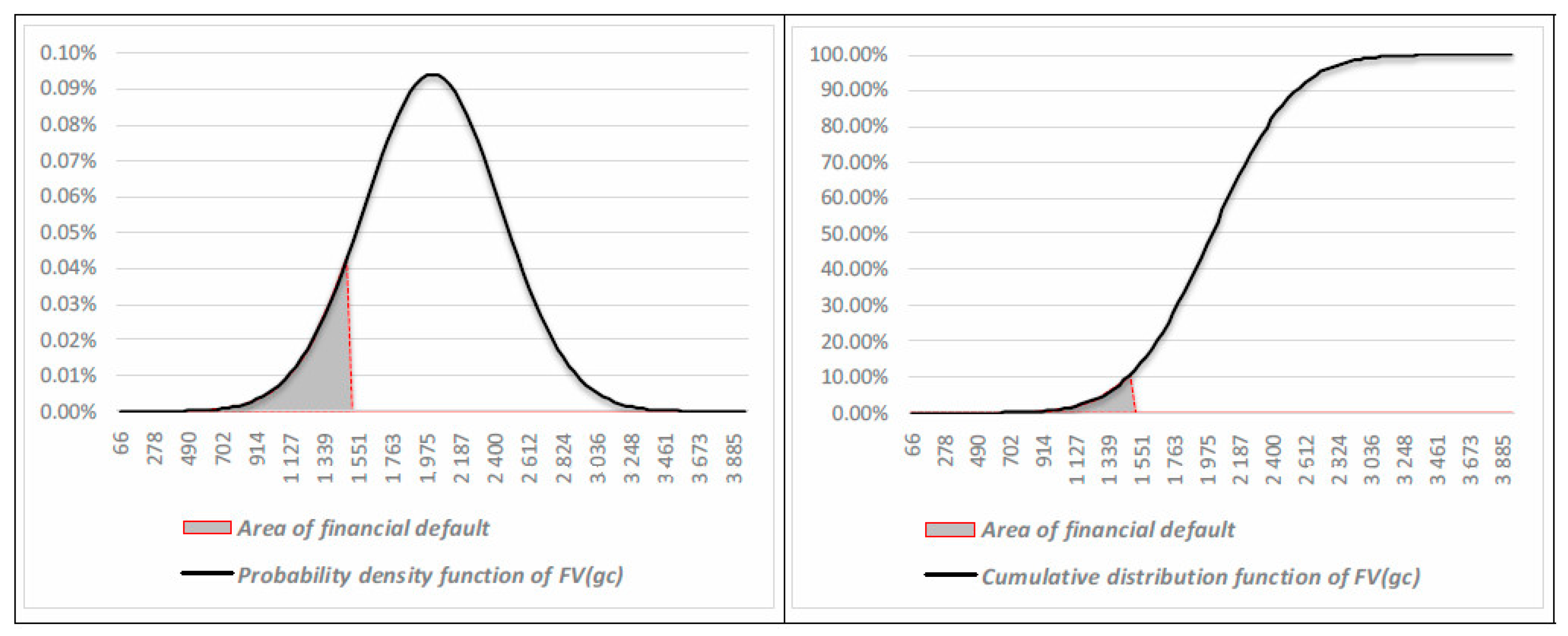
The default risk emerges by considering whether the operating results are sufficient over time to repay and remunerate financial debts. This condition could be analyzed in terms of present values of assets and debts: the going concern is economically and financially sustainable when the economic value of firm assets (The “economic value” corresponds to the present value of future cash flows generated by the asset in place and growth opportunities, considering an “ongoing concern” hypothesis.) (FVgc) is equal to, or higher than, the face value of the financial debt (FD). A lower FVgc than FD indicates an excess of debt, which absorbs much more cash flow than that the core business can structurally generate.
The assessment of the economic values’ dispersion, in a going concern hypothesis, allows for the measurement of default risk. A stochastic approach requires us to consider FV as a random variable for which a probabilistic distribution is assumed. In this way, the CaR can be calculated as the difference between the estimated value of a firm (the expected value of a probabilistic distribution of alternative values), and its economic value corresponding to a given confidence level:
The CaR indicates the expected loss of the firm’s economic value due to the fact that competitive scenarios may arise in which the firm, while maintaining the going concern, will generate unsatisfactory financial performances. If the residual firm value is lower than the outstanding financial debt, both shareholders and creditors would have no interest (except in the case of a moral hazard) in the going concern; they could then take action to put the company into a restructuring process or a liquidation process (A firm value lower than financial debt indicates, in a going concern scenario, returns on equity lower than the cost of equity. This could lead the shareholders to opt for a business interruption and a corporate liquidation.).
The equity capital that should be allocated to cover the risk of restructuring or a business interruption should be quantified by moving from the CaR to a peculiar measure of Economic Risk Capital (ERC). Assuming that FV, in a going concern scenario, cannot be less than zero, an optimal level of equity risk capital, ERCα, given a certain confidence level, will be:
Optimal ERC is a function of the financial leverage and the variability in FV, which depends on the variability of CFF, the cost of capital, and the company lifetime:
Annual cash flows to firm depend on Ebitda, taxes, changes in net working capital, and capital expenditures:
Indicating the Ebitda after taxes as Ebitda*, the variance in CFF could be expressed as follows:
Definitely, ERC also depends on:
- -
- market dynamics, the operating leverage degree, fiscal policies;
- -
- working capital management and commercial policies;
- -
- investment policies;
- -
- financing policies; and
- -
- the degree of independence of investment and financing policies with respect to operational and working capital management choices.
Therefore, since the available equity risk capital is the net worth, the needs (or surplus) of equity risk capital, ERCts/n, will be:
Notice that a risk capital lack may not require a corresponding equity capital increase. If the net invested capital remains flat, a full coverage of the business interruption risk requires approximately additional equity—to replace debt—equal to half of the estimated risk-capital needs.
Similarly, ERCs/n implicitly provides information on the probability of financial default in a going concern scenario (see Table 2).
Given a certain likelihood of business interruption, the firm’s solvency in a liquidation process is still guaranteed when the current value of assets (FVlc), reduced by potential liabilities, is overall equal to, or higher than, the FD. The current value corresponds to the sum of market value, obtained through “fire sales”, of each asset in place considering a “liquidation” hypothesis. In such a scenario, a risk capital measure must indicate the equity necessary to guarantee the repayment of financial debts through a total asset liquidation. This explains why FV must be also estimated in a liquidation hypothesis. In this case, the CaR is defined as the difference between the estimated value of a firm (the expected value of a probabilistic distribution of alternative liquidation values) and its liquidation value corresponding to a given confidence level:
In this case, CaR indicates the expected loss of the firm’s value due to the liquidation process. If the loss in asset value is such that the residual firm value is lower than the outstanding financial debt, a risk of potential bankruptcy emerges. To quantify the capital that should be allocated to cover this risk, the specific measure of Economic Risk Capital (ERC) will become the following:
Since the equity capital is the right buffer to cover the expected economic losses in a liquidation process, the surplus or needs of ERC will be:
Once again, ERCs/n implicitly provides information on the probability of bankruptcy in a liquidation scenario (see Table 3).
In order for risk-based capital measures to be useful in setting up decision-making models for corporate financing policies, a firm should adopt:
- (1)
- forecasting methodologies (for budgeting and planning) coherent and connected with the VaR logic; and
- (2)
- valuation methods that explicitly consider the risks and costs of insolvency.
(1) When the VaR logic is applied to calculate LRC and ERC, two main choices are needed: the approach to the expected losses (parametric or non-parametric); and the form of probability distribution (normal, log-normal, binomial, etc.). Such choices affect (even significantly) the measure of risk-capitals and must be consistent with the forecasting procedures (Monte Carlo or scenario; build-up or pure probabilistic) adopted by the firm. The build-up approach requires us firstly to calculate the mean expected values of the elementary variables (revenues, costs, BCC, etc.), and then to determine the financial results by composing those expected values. The pure probabilistic approach requires us firstly to calculate the alternative financial results in each scenario, and then to determine the mean expected values.
Financial planning and budgeting must clearly consider the variability in the expected flows in each period within the forecasting horizon (short-term, medium to long term). To depict the probabilistic distribution of expected cash flows, different approaches are available. The “scenario approach” is normally associated with a representation of alternative cash flows in a limited number of scenarios (normally the triad “pessimistic–expected–optimistic”), each of which is attributed a (subjective) probability of occurrence. In this case, the results are affected by the decision maker’s discretion in assessing the company’s ability to adapt to various contexts (alternative scenarios) and to achieve the planned results. The “Monte Carlo approach” is instead based on random generation procedures that give lots of values for each of the elementary variables that determine the expected cash flows. In this case, the results depend on how either the behavior of the input variables (normal or non-normal; subjectivist or frequentist probability distribution), the correlations between the input variables, and the cause–effect relationships (linear or non-linear) are defined. Although the “Monte Carlo approach” allows us to better simulate the continuity of a firm’s variables and values, the “scenario approach” allows us to better represent the firm’s flexibility and resilience within unfavorable competitive conditions.
The VaR methodology allows for both a parametric and a non-parametric approach. The first one has the limit of approximating with linear relationships the real (non-linear) relationships between financial figures and risk factors. However, it also has the advantage of simplicity: the average and standard deviation of expected results are sufficient to describe the shape of the probability distribution of the variables considered. Therefore, the parametric approach allows us to apply the VaR methodology in a subjectivist perspective; that is, through: the construction of alternative scenarios, the assignment of subjective probabilities of occurrence, and the calculation of variability indexes of relevant results and values.
(2) Any deficit or surplus in risk capital should guide the firm’s financial policies and suggest to the Chief Financial Officer proper adjustments to the capital structure. However, the resulting optimization process cannot only consider the minimization of the insolvency risk but also the related effects in terms of firm value. Indeed, variations in the liquidity degree of assets change the risk and profitability of the net invested capital, and variations in financial leverage change the cost–benefit tradeoff of financial debts. Therefore, the search for an optimal capital structure is a problem of a continuous search for balance between the insolvency risk consistent with the expectations of lenders and the value creation prospects consistent with the expectations of shareholders.
3.4. Firm Value and Insolvency Risk
Consistently with financial theory, it must be considered that a financial distress involves costs related to financial restructuring procedures, while a financial default involves costs related to bankruptcy procedures. In a going concern hypothesis, the distress (direct and indirect) costs, whose incidence on firm value is δd, will occur with a probability of pd; the firm value will be:
In a liquidation hypothesis, the bankruptcy (direct) costs, whose incidence on firm value is δb, will occur with a probability of pb; the firm value will be:
Therefore, the firm value will be a weighted average between the going concern value and the liquidation value, where the weights are based on the probability of default.
4. Scenario Analysis and Simulations: Methodology and Results
The validation of the risk capital measures proposed above appears complex through empirical analysis. While it would be useful to test the effectiveness of LRC and ERC on actual firms, the nature of risk-capital measures makes an empirical analysis difficult to carry out. Such an analysis would require information on forecasting data (plans and budgets) and on the financial flexibility of a company. Any information lack could influence the estimation of LRC and ERC and the assessment of their effectiveness. Moreover, deriving the performance variability from historical trend analysis may not allow us to take into account the strategic/operating flexibility separately from financial flexibility, the firm’s approach to risk management, and other relevant variables.
For this reason, it appears appropriate to approach the check of the usefulness of LRC and ERC through a forecasting and simulation model that allows for analyzing the effects of the variability in operating cash flows on liquidity and solvency. Expected cash flows are estimated based on the following equations:
with:
being:
- -
- Revt the turnover in period t (month or year);
- -
- ϖ the variable operating costs on revenues ratio;
- -
- Foct the fixed operating costs; and
- -
- τ the corporate tax rate.
By applying the Equation (17), expected Ebitda* are estimated in various alternative scenarios, each characterized by a different growth rate of revenues. We assume the invariance of ϖ and τ (fixed costs are invariant by definition) among the different scenarios; in this way, the variance of Ebitda* depends on the variability of revenues, and its magnitude is explained by the operating leverage and the tax rate:
Recalling then the Equation (16), the assumptions of invariance of working capital policies and independence of investment policies from revenues’ variability make the VARCFF strictly dependent on the variability of revenues. The distribution of alternative revenue growth rates is modeled through a Monte Carlo simulation, assuming a normal form of probability distribution and making a specific hypothesis about the mean and standard deviation of the growth rate. Therefore, the simulation and forecasting model focuses on the effects of the main source of business risk (uncertainty of sales) on firm liquidity and solvency, allowing us to size the risk capital with respect to this factor of risk.
In each alternative scenario, financial budgets and financial plans reflect the outcomes of the forecasting model; the same model is used to simulate the effects on a firm’s cash flows, the liquidity and solvency of the alternative hypothesis of capital structure (4), and financing strategies (3).
The analyses and comparison of the results obtained by combining alternative capital structures with alternative financing strategies (12 combinations) allow us to verify the behavior of LRC and ERC and their usefulness in reducing the risk and probability of insolvency.
4.1. Parameter Values
The model simulates the financial plan (5 years) and the treasury budget (12 months) of a firm with the following operating characteristics: an annual capital turnover of 90%; variable costs on revenues of 40%; fixed costs on net invested capital of 35%; a depreciation rate for fixed assets of 10%; annual capital expenditure equal to annual depreciations; Days Sales Outstanding equal to 60 days; Days Payable Outstanding equal to 30 days; and a tax rate of 25%.
The expected earnings and cash flows at the end of each year were obtained through a Monte Carlo simulation assuming a normal distribution for the growth rate, with the mean and standard deviation shown in Table 4.
The random revenue generation process provided 1000 alternative annual growth rates, each of which is attributed a probability of occurring on the basis of its frequency (see Figure 1).
The forecasting model also considers seasonality to model the financial budgeting (see Table 5).
4.2. Base Case
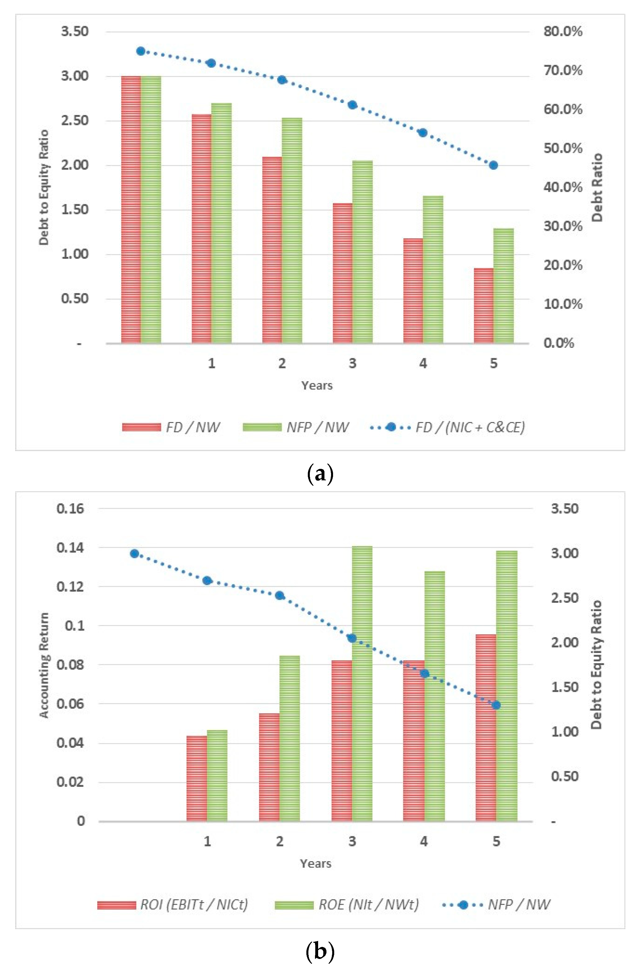
The capital structure of the firm is initially composed by equity (25% of the Net Invested Capital, NIC) and long-term financial debt (75% of the NIC). The financial debt is a bond with a maturity of 10 years, an annual interest rate of 3.5%, and monthly installments with constant principal repayments. The initial financial leverage changes over the years in the planning horizon (see Figure 2a), at the same time influencing the dynamic of Roe (Figure 2b).
For each period, the expected value and the probabilistic variance and standard deviation of economic results (see Table 6a) and financial results (see Table 6b) were calculated. The financing policies affect both the level of mandatory repayments on debt and their covariance with CFFs, as well as debt reserves.
The firm valuation is run in each scenario through the DCF model assuming an asset-side perspective and adopting the APV procedure; the unlevered cost of capital (ku) is estimated using the CAPM with a risk-free rate of 2.0%, a market risk premium of 6.5%, and an unlevered beta of 0.9. The expected value in a liquidation hypothesis, which represents a “floor” for the potential losses of creditors, was estimated considering a depreciation rate of fixed assets of 25% and a loss on expected receivables of 40%.
Company values (FV), share values (EqV), implicit multiples, and their variability (see Table 7) do not consider default costs, which will be introduced later.
Since the expected cash flows and economic values are random variables that move continuously, it is assumed that:
- -
- the expected value and the standard deviation are representative of the entire distribution of flows and values; and
- -
- these distributions are continuous, normal, and symmetrical consistently with the assumption on the revenue’s distribution.
The VaR logic allows us to measure the areas of insolvency underlying the distributions of firm values, thus defining the probability of default in a going concern hypothesis (see Figure 3), and of bankruptcy in a liquidation hypothesis (see Figure 4).
The risk-based measures relevant to the treatment of insolvency risk were estimated both in a going concern hypothesis and in a liquidation concern hypothesis: Capital at Risk (CaRα) applying Equations (7) or (10), Equity Risk Capital (ERCα) applying [8] or [11], and Equity Risk Capital Needs/Surplus (ERCn/s) applying Equations (9) or (12). All the measures were determined considering a holding period of 1 year and a confidence level of 95% or 99% (Table 8).
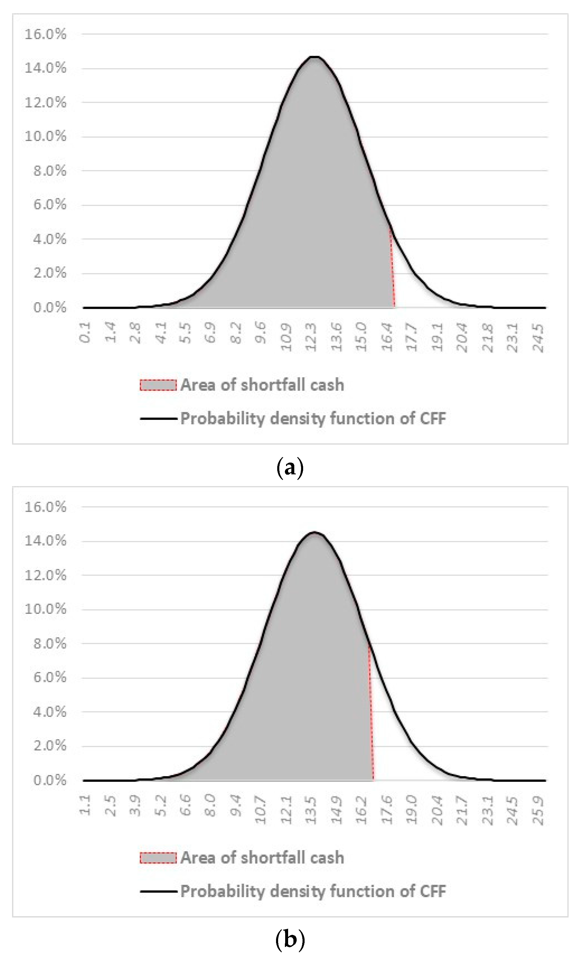
Moving to the short-term analysis, the simulation model allows us to estimate the probability that a situation of financial distress will occur, and to measure the risk capital needed to deal with such a situation. Analyzing the variability in monthly CFF and FSN, it emerges that the probabilities of a shortfall in cash and financial distress vary throughout the year because of the variability and seasonality of the expected revenues. For example, the shortfall in cash risk and financial distress risk are higher in March (see Figure 5a) than in May (see Figure 5b).
The monthly CFF and FSN were calculated by applying Equations (16) and (17), while the CFaR was calculated by applying Equation (1) in two different hypotheses of confidence level (see Figure 6a) along with the related probabilities of financial distress (see Figure 6b).
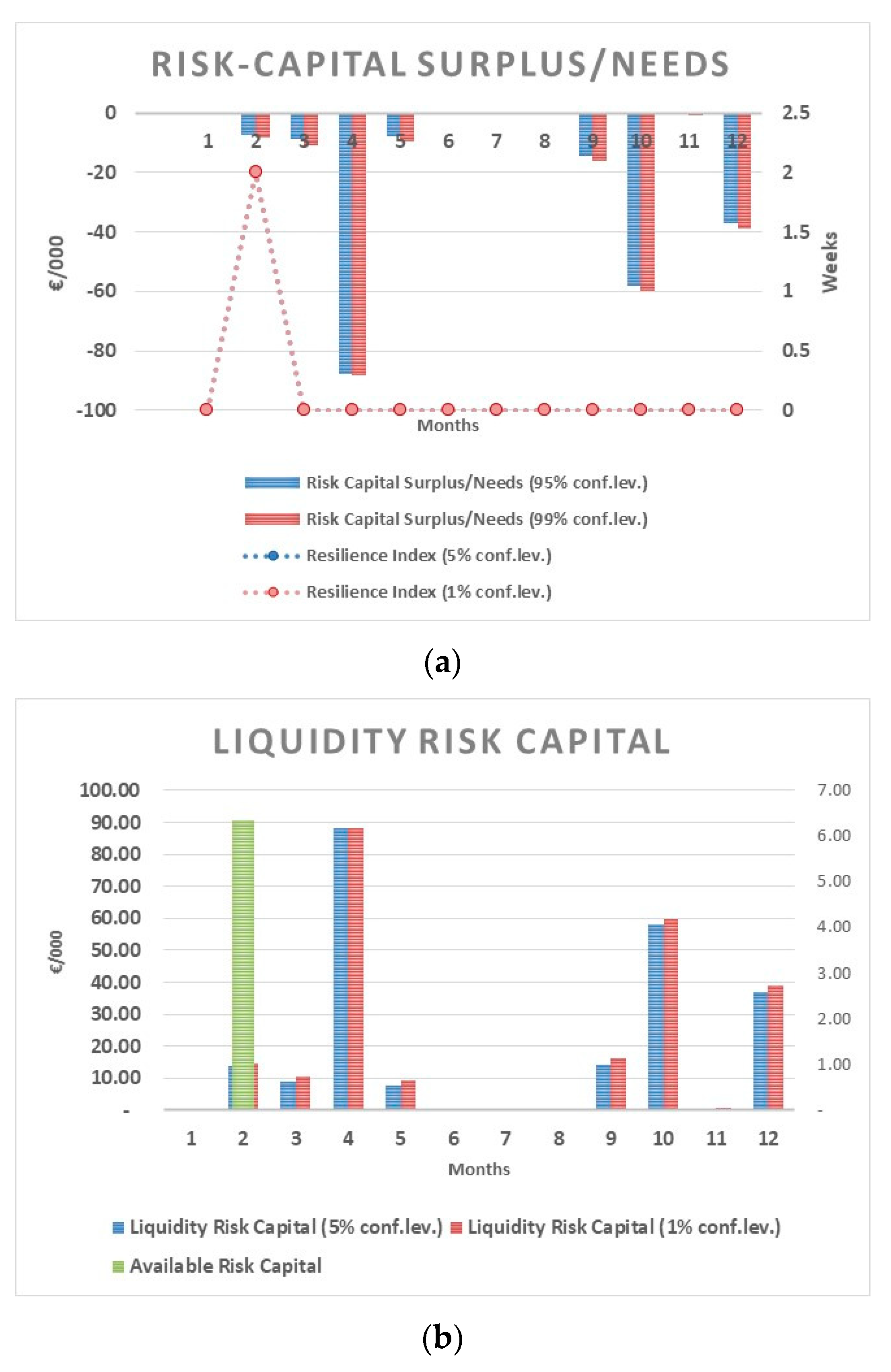
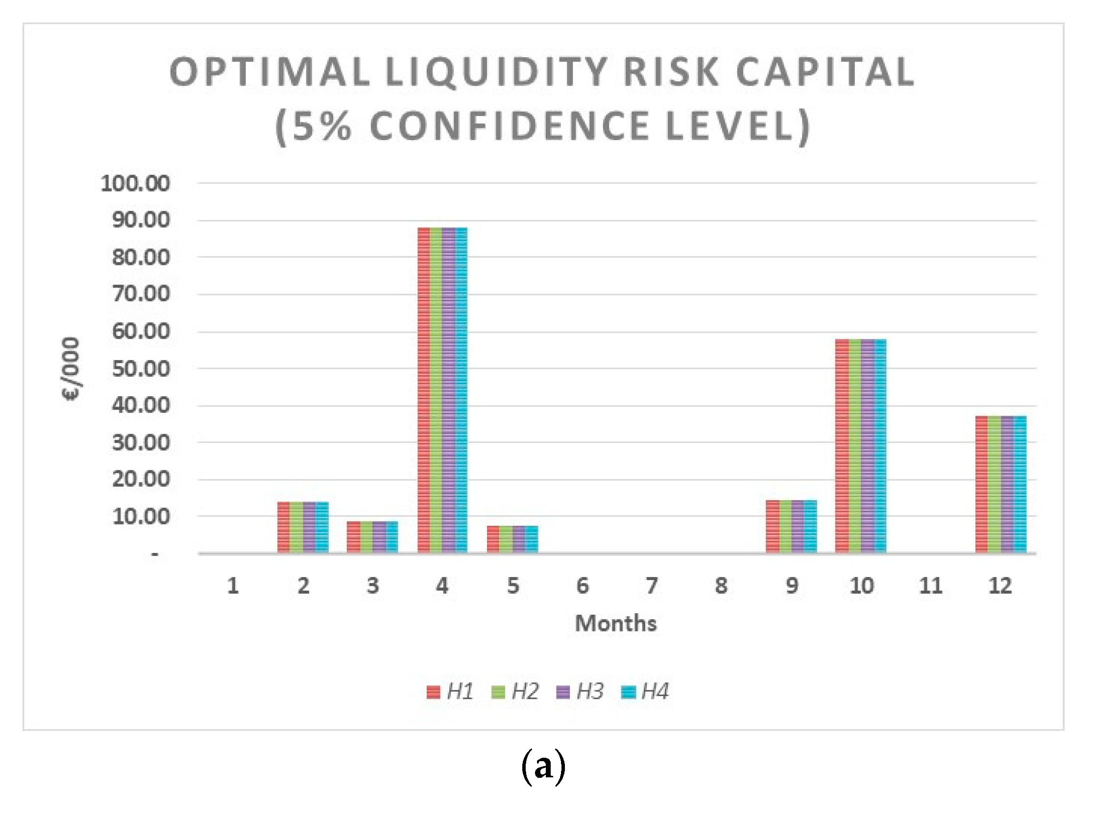
In other terms, the firm’s financing policy is not coherent with the seasonality and the variability of revenues, leading to a situation of financial distress at the beginning of the second quarter of the year. The risk-based measures relevant to the treatment of liquidity risk were then determined considering a holding period of 1 month, a confidence level of 95% or 99%, the Liquidity Risk Capital (LRCα) applying Equation (3), the Available Liquidity Risk Capital (LRCav) applying Equation (4) (see Figure 7b), the Liquidity Risk Capital Needs/Surplus (LRCn/s) applying Equation (5), and the Resilience Index applying Equation (6) (see Figure 7a).
4.3. Simulations
While the probability of default is relatively low, the scenario analysis shows that the capital structure of the firm should be modified to avoid a condition of financial distress. This can be obtained through several actions, keeping unchanged the net invested capital. Those considered in the simulation are (Table 9):
- -
- a reduction in financial debt offset by a correspondent increase in equity (first strategy, S1);
- -
- a reduction in net financial debt due to an increase in liquidity obtained through an equivalent increase in equity (second strategy, S2); and
- -
- an increase in short-term debt keeping unchanged the overall financial debt, with creation of debt reserves (third strategy, S3).
4.3.1. First Financing Strategy (S1)
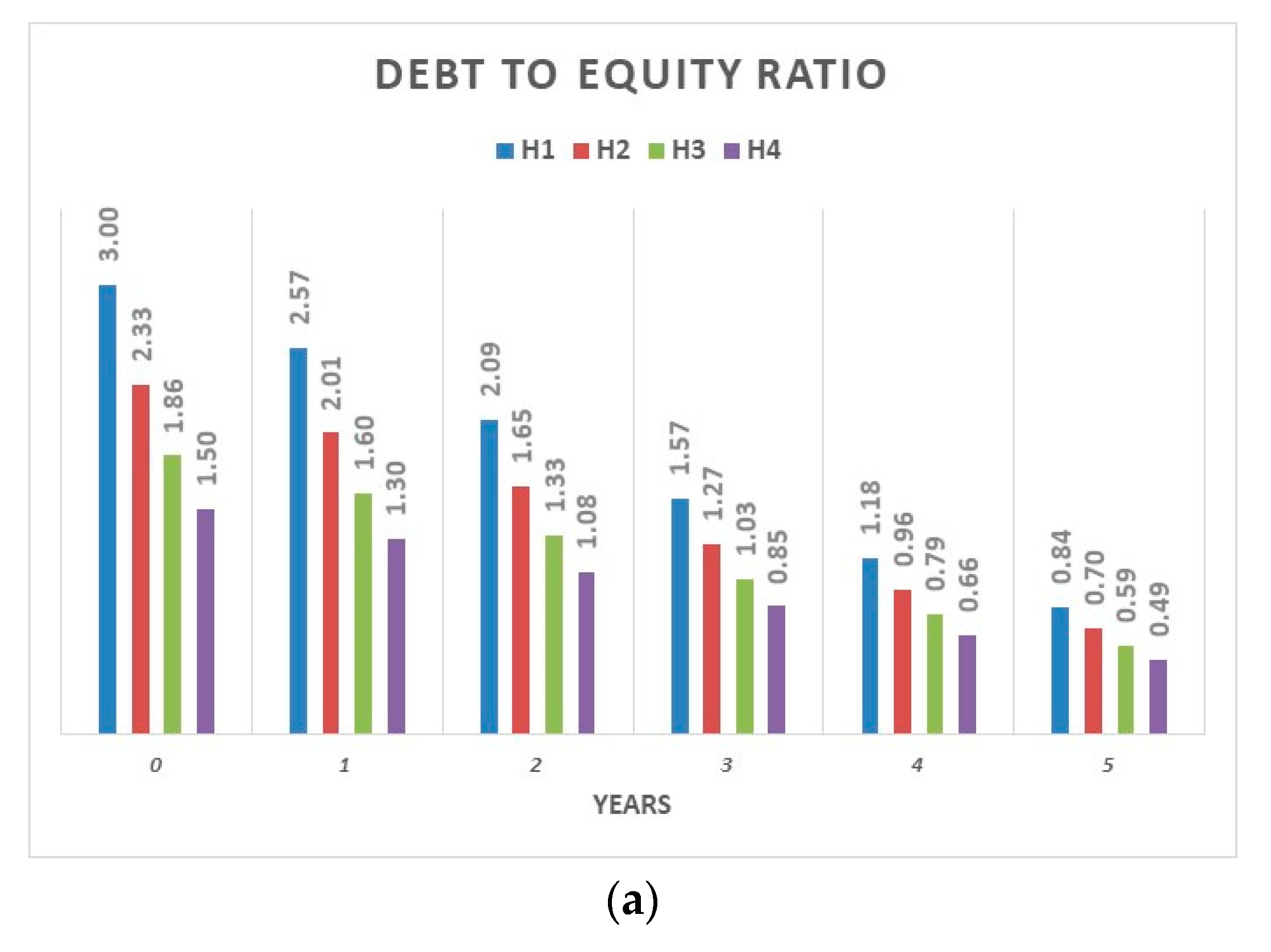
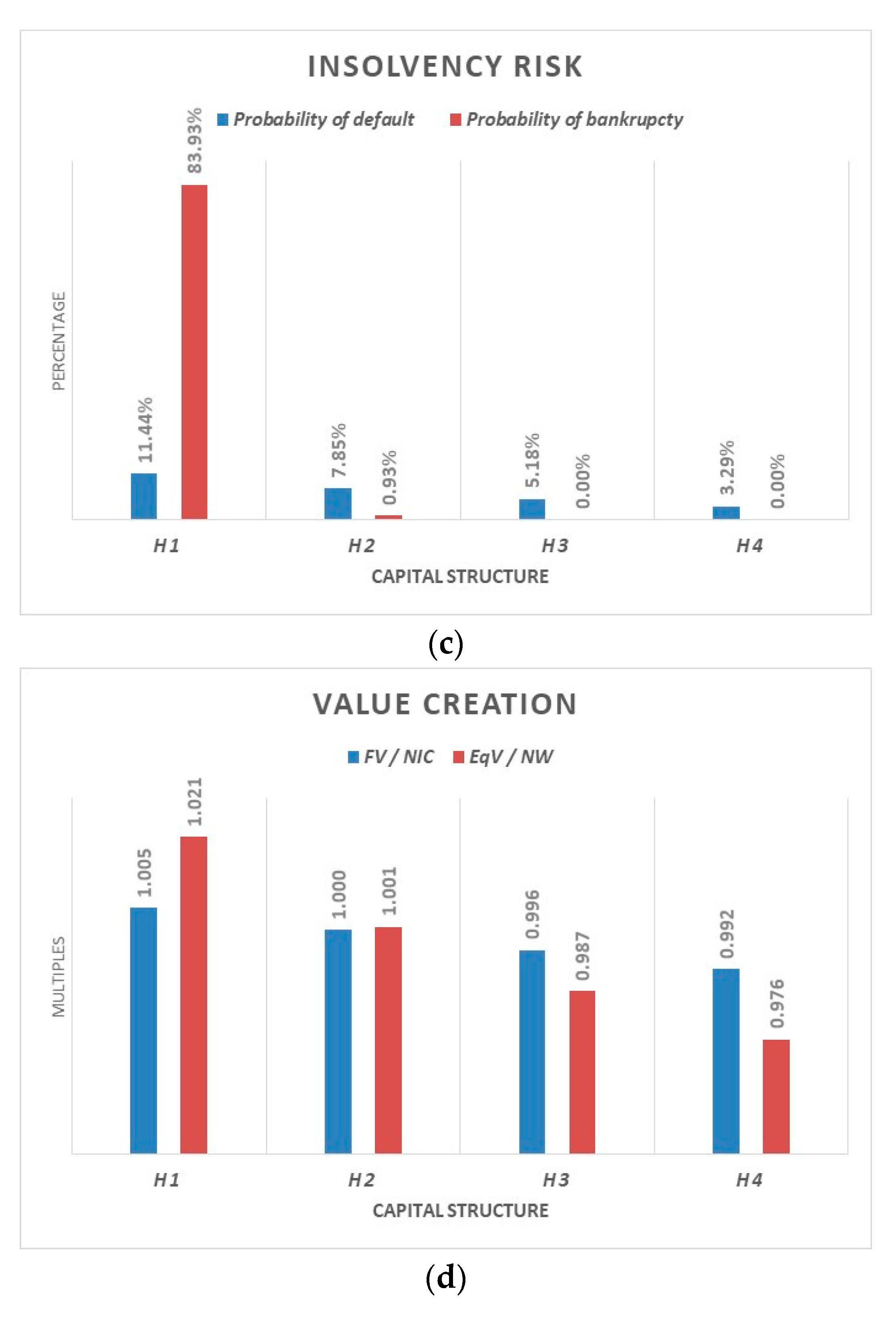
The first simulation considers three different hypotheses of capital structure, which are alternatives to the initial one. A reduction in financial leverage involves (see Figure 8a): the transition from a lack of equity to a high surplus (see Figure 8b); a significant reduction in the probabilities of default and bankruptcy (see Figure 8c); and a slight reduction in both asset-side and equity-side multiples (see Figure 8d).
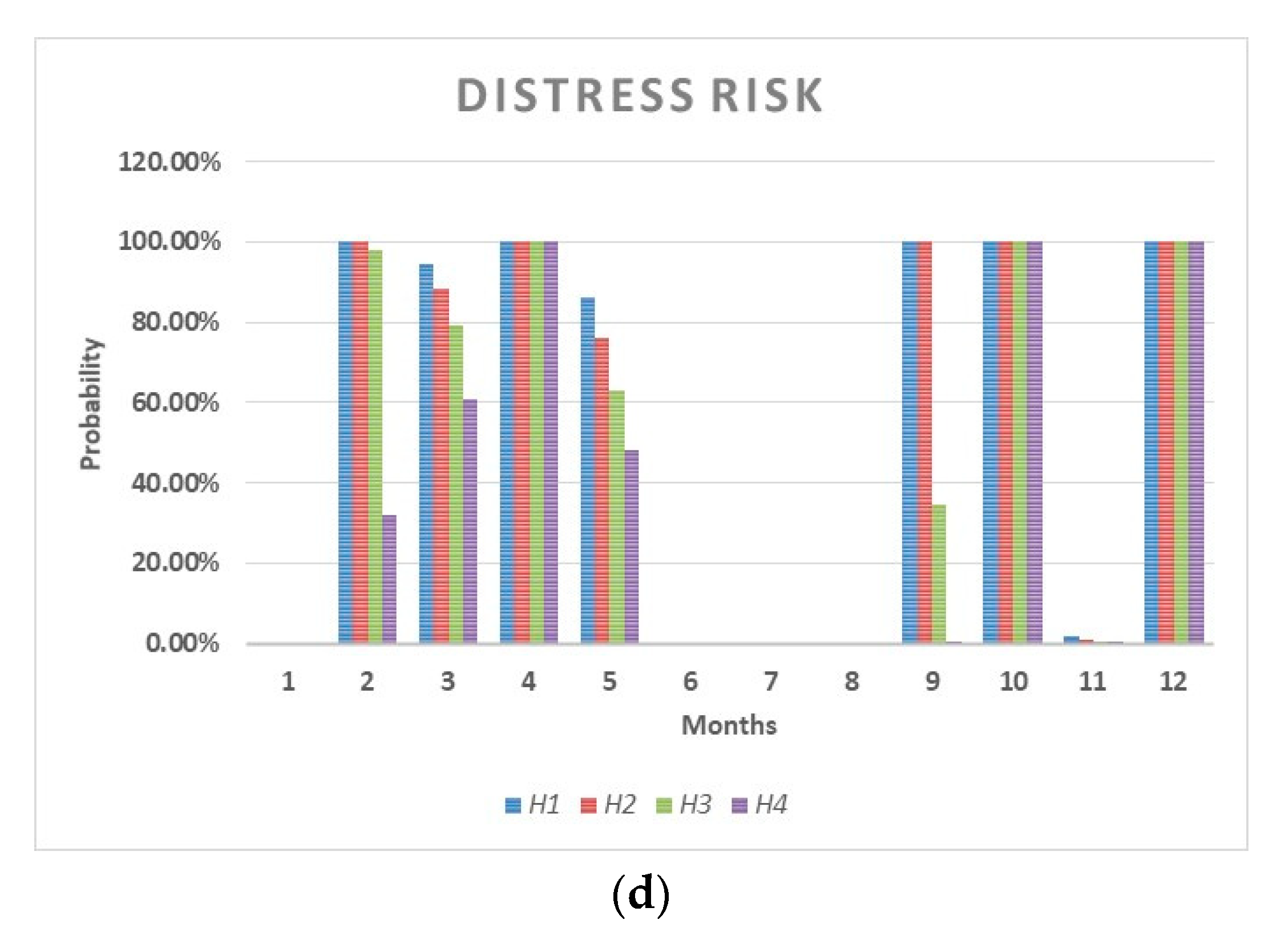
A financial strategy exclusively based on a reduction in financial debt, on the one hand, reduces the probability of default and eliminates that of bankruptcy, but, on the other hand, it involves a significant reduction in value creation for the shareholders. Furthermore, this financial strategy is not effective in reducing the risk of financial distress (see Figure 9a,c); in fact, the need for liquidity risk capital (see Figure 9b) is reduced very little and the certainty of the financial distress in February remains (see Figure 9d).
4.3.2. Second Financing Strategy (S2)
The second simulation considers a progressive reduction of net financial leverage, obtained not through a financial debt reduction, but an increase in cash and cash equivalents corresponding to an increase in equity (see Figure 10a). This strategy has similar impacts on risk capital (see Figure 10b), probabilities of default or bankruptcy (see Figure 10c), and value creation (see Figure 10d).
4.3.3. Third Financing Strategy (S3)
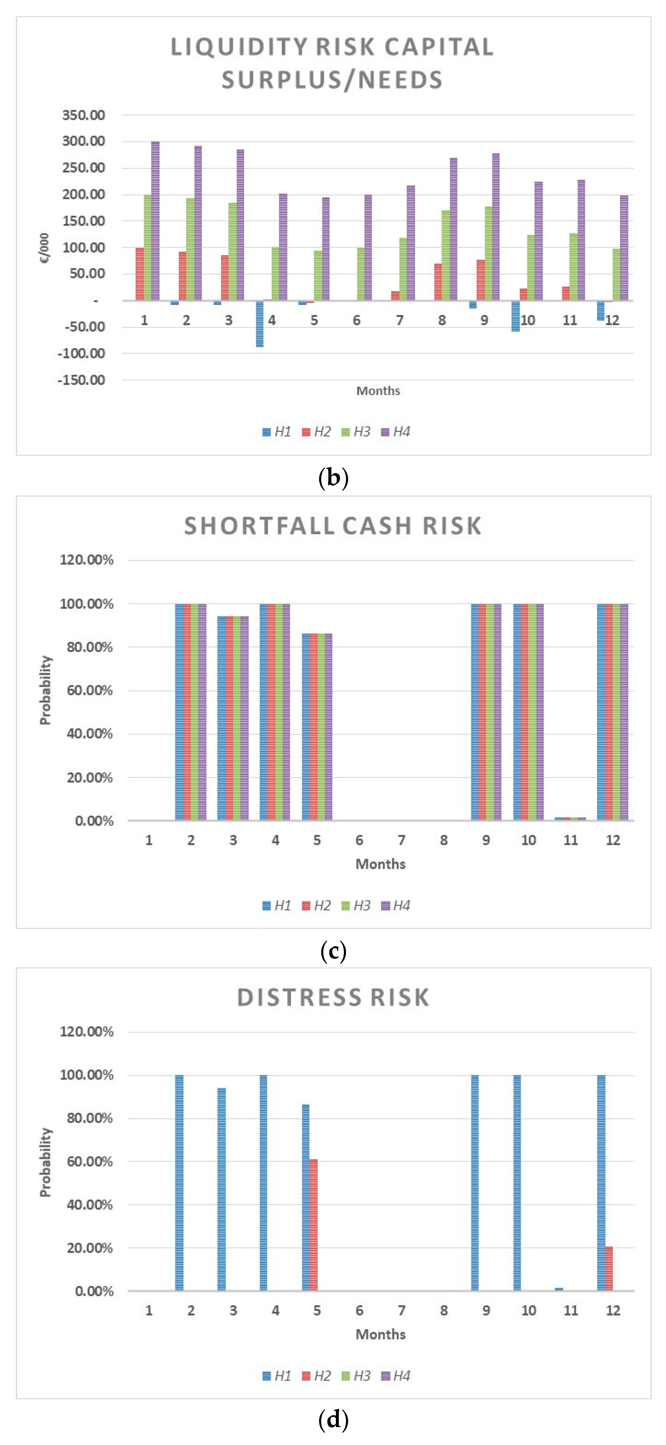
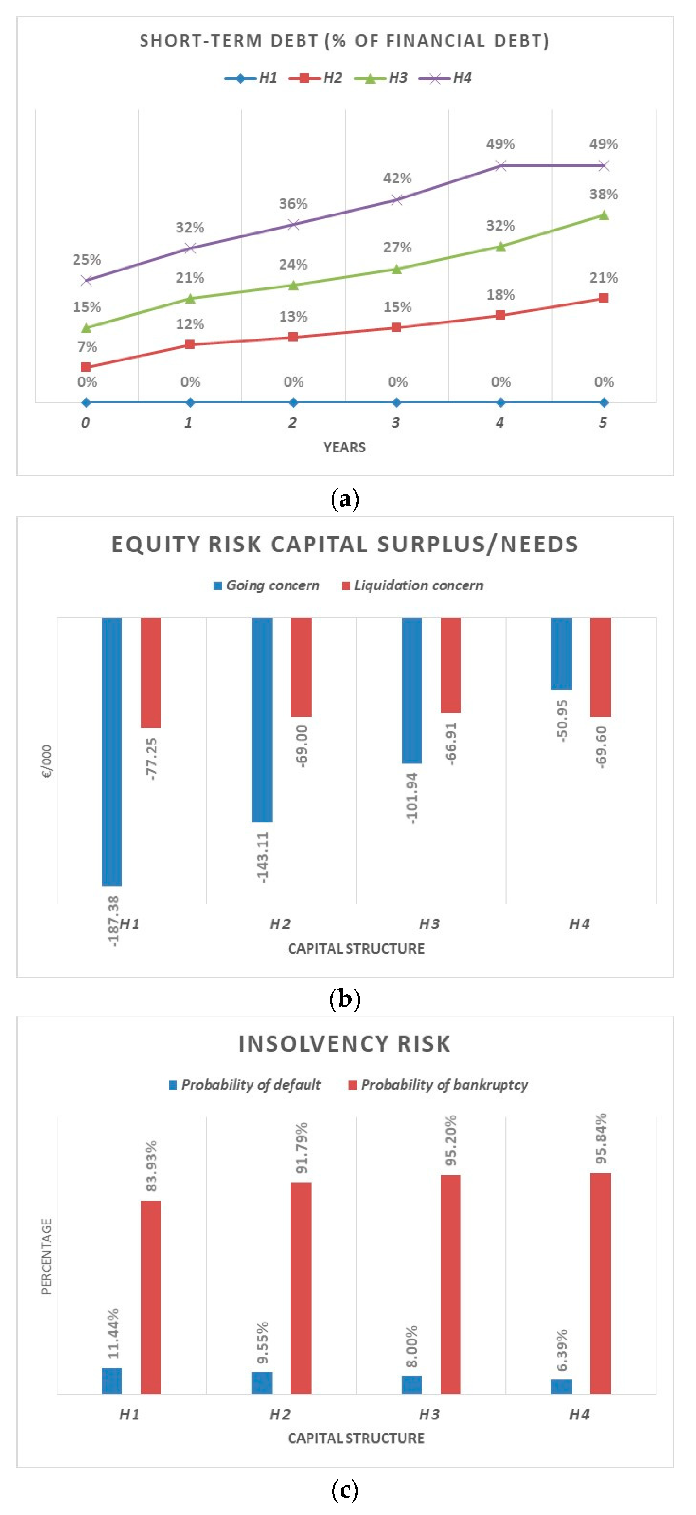
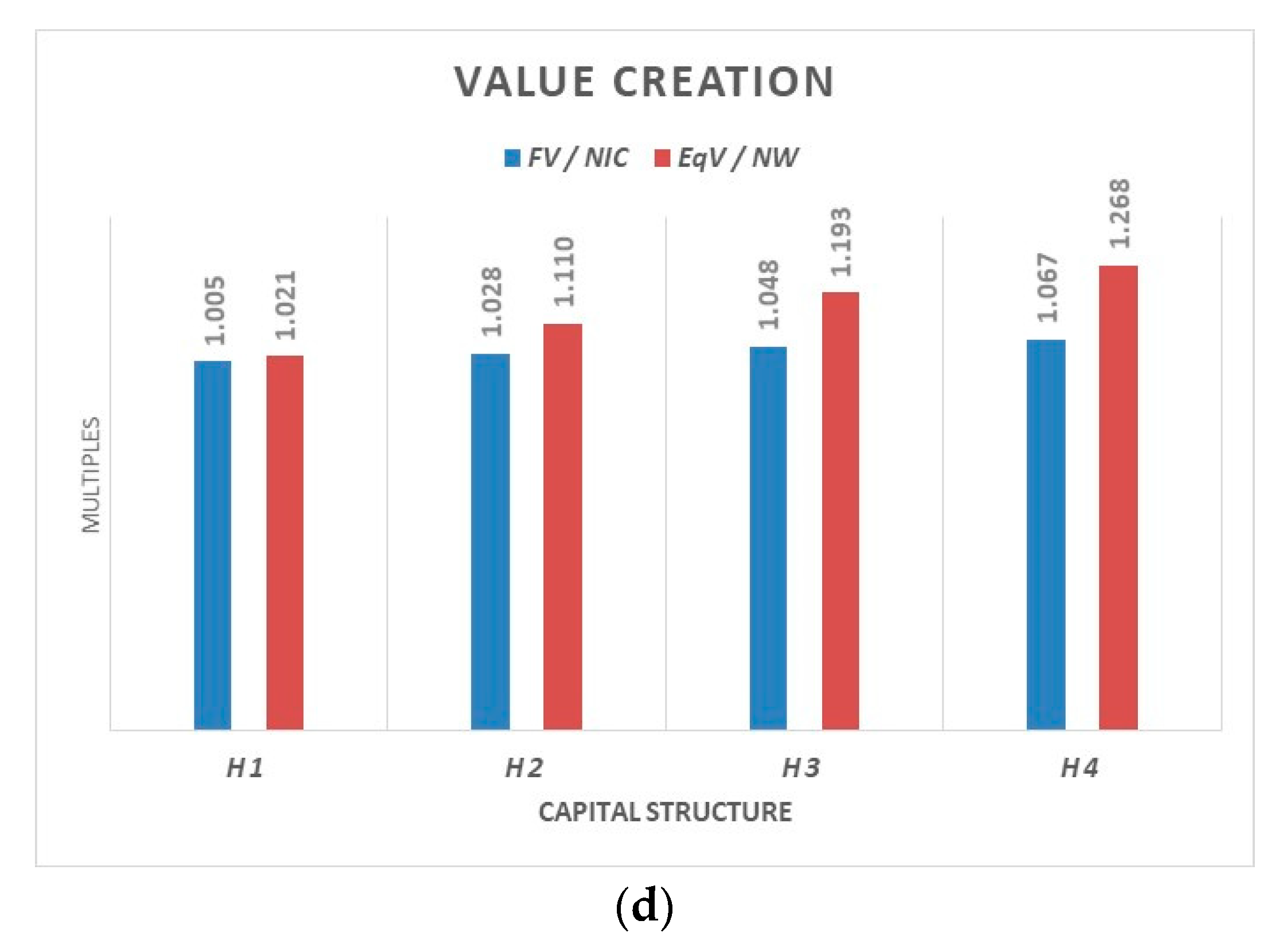
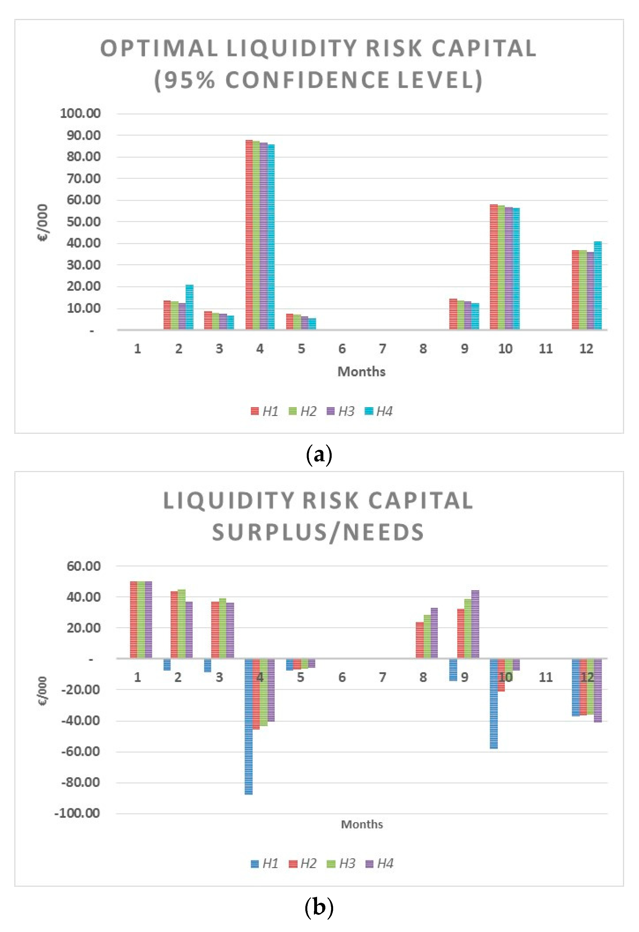
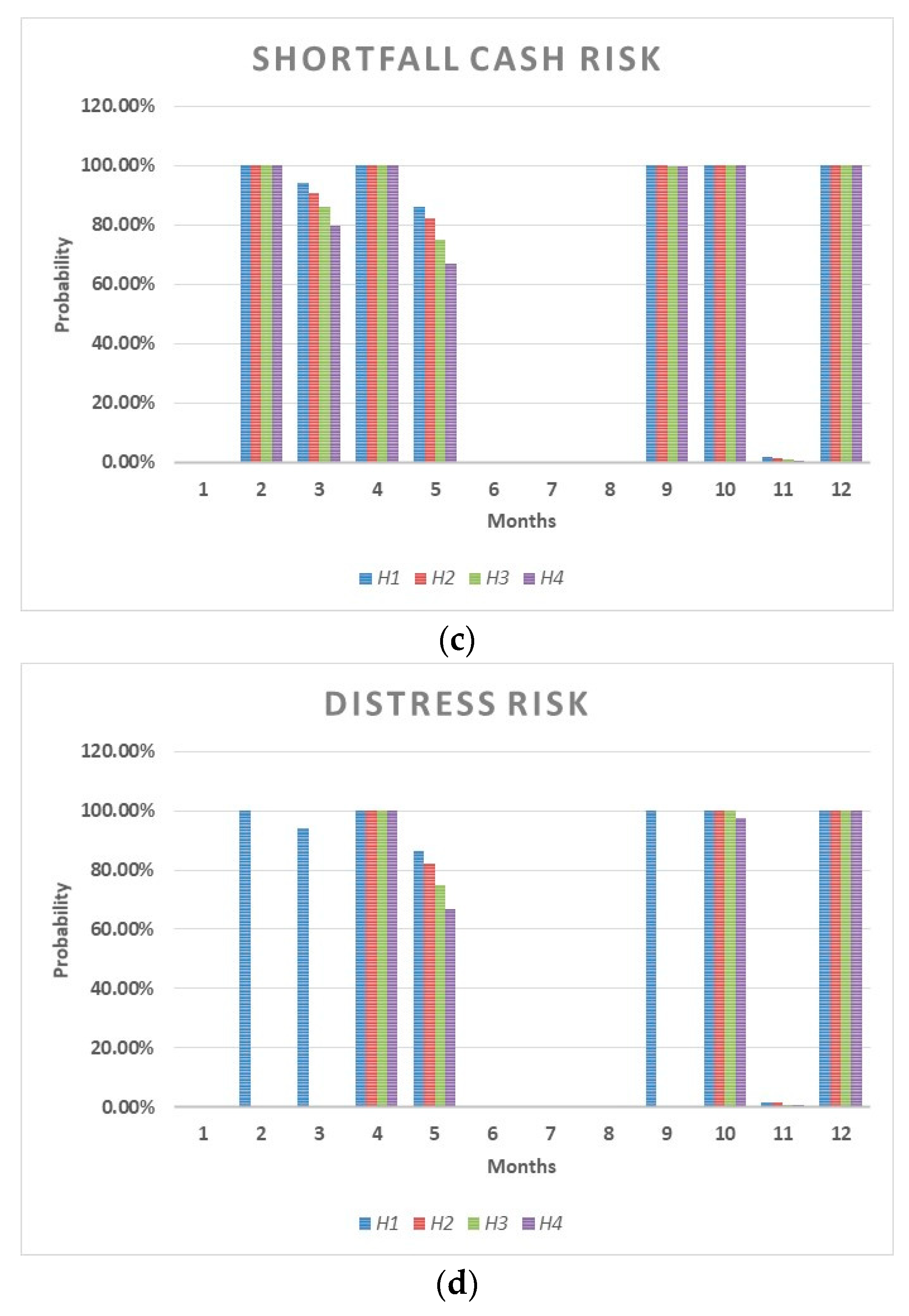
The third simulation considers a gradual increase in short-term debt, while the overall debt remains flat (see Figure 12a). The short-term debt consists of: a credit line for advance invoices that increases up to a maximum of 150 k/€ with an annual interest rate of 6%; and an ordinary line of credit that increases up to 150 k/€ with an annual interest rate of 6%. Compared with the previous simulations and hypotheses, this strategy allows us to limit risk of default (see Figure 12c) and to increase the value creation (see Figure 12d), but it does not reduce the risks of bankruptcy and the lack of ERC in a liquidation scenario (see Figure 12b).
In this case, a condition of financial distress will occur with certainty during the first year (see Figure 13c,d); indeed, this financing strategy has no relevant effects on the reduction of liquidity risk-capital needs.
5. Discussion of Results
The comparison of the different financial strategies clearly shows that, given the business conditions assumed above, changes in the financial structure allow us to optimize the liquidity or equity risk-capital, reducing the insolvency risk. However, adjustments in equity risk-capital allow us to reduce/eliminate the probability of default/bankruptcy, but do not allow us to reduce the probability of financial distress, which instead requires adjustments in liquidity risk-capital.
The financial strategy S1 produces a significant reduction in the default probability, but no reduction in the distress probability. Thanks to a net financial leverage (NFD/NW) reduction from 3.00 to 1.50 (−50.50%), the probability of default reduces from 11.44% to 4.16% (−63.64%), and the probability of bankruptcy reduces from 83% to 0% (−100%). However, this does not eliminate the condition of distress that occurs in the first year of the plan (in February, a distress probability of 100%). The financial strategy S2 produces similar effects on the default risk, but it significantly reduces the first-year distress risk. When the reduction in net financial leverage is obtained by an increase in the firm’s liquidity, the risk of financial distress in the first year of the budget is eliminated. The financial strategy S3 does not produce significant effects either on the default risk nor on the distress risk. The greater flexibility of the financial structure together with debt reserves are not sufficient to reduce the overall insolvency risk.
Moreover, if there is seasonality, the financial structure assessment and optimization always require combining a short-term analysis with a medium to long term one. Notice that the distress probability on an annual basis differs from those calculated on a monthly basis.
The effects of the three financial strategies can be also observed through the dynamics of LRC and ERC. Their needs or surplus make it possible to optimize the firm’s capital structure and avoid excessive or insufficient changes in leverage with respect to a specific risk target. The simulation’s results show that any surplus of equity risk-capital does not generate significant reductive effects on firm value, while it generates significant effects on equity value. When the direct and indirect insolvency costs are nil (as per the hypothesis underlying the previous simulations), the excessive equity risk generates reductions in equity value. Furthermore, the balance between insolvency risk and economic value is obtained by combining several financial strategies to avoid excessively reducing debt and losing the related tax benefits.
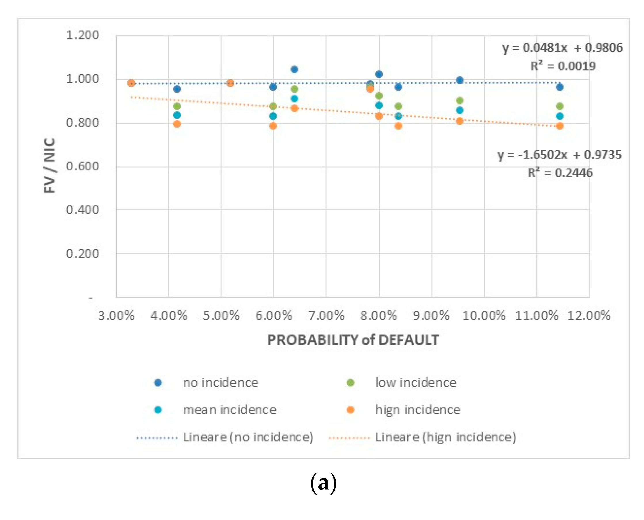
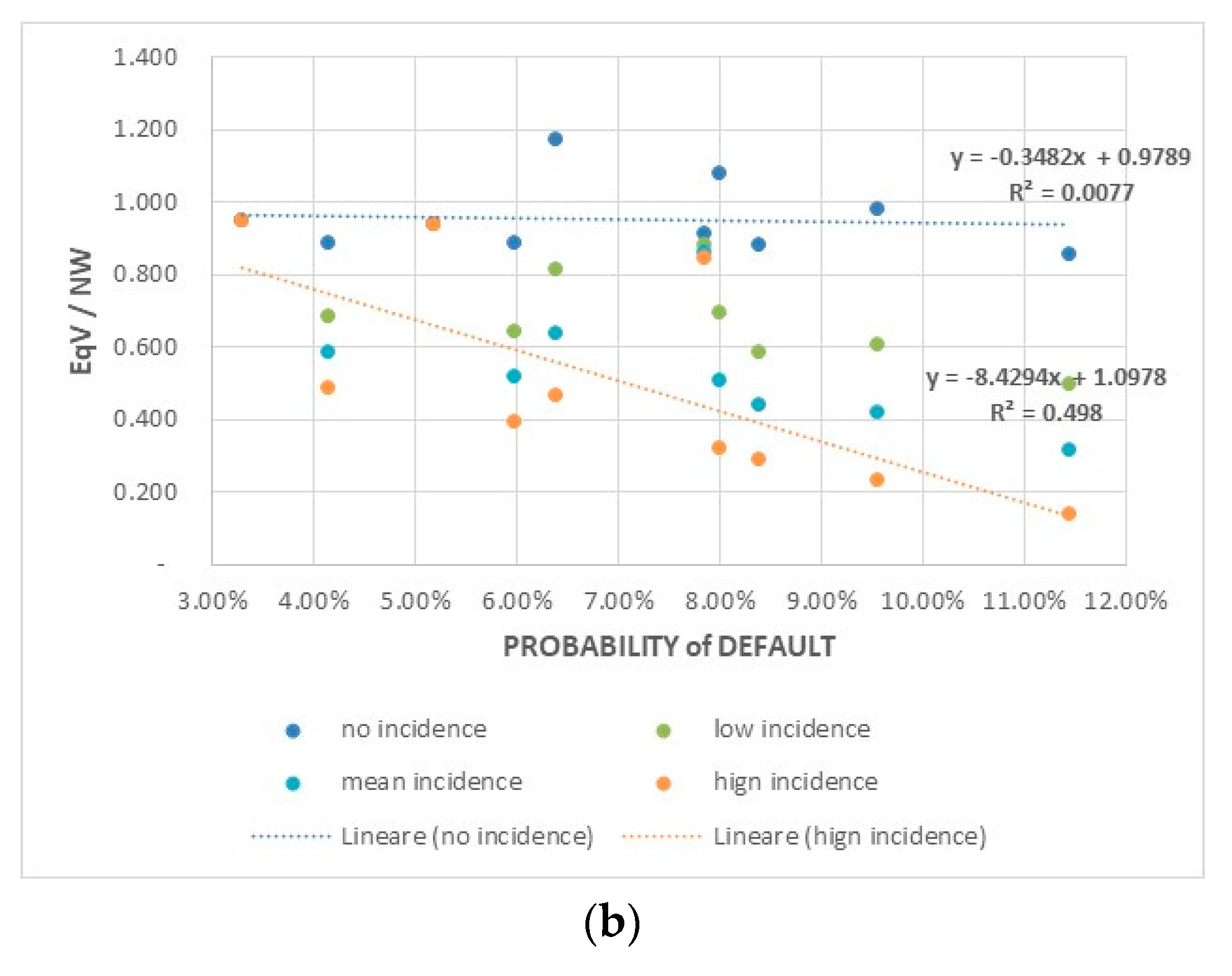
Comparing the three financial strategies is useful to highlight correlations between the probability of distress or default, a surplus/an excess in liquidity or equity risk capital, and the creation of firm value and equity value. We considered an increasing cost of default: four incidences of distress costs on the economic value (zero, 0%; low, 10%; medium, 15%; high, 20%) and four incidences of bankruptcy costs on the liquidation value (zero, 0%; low, 3 %; medium, 4%; high, 5%) are assumed.
For each hypothesis of default costs, the economic value, liquidation value, and firm value were calculated by applying Equations (13–15), respectively.
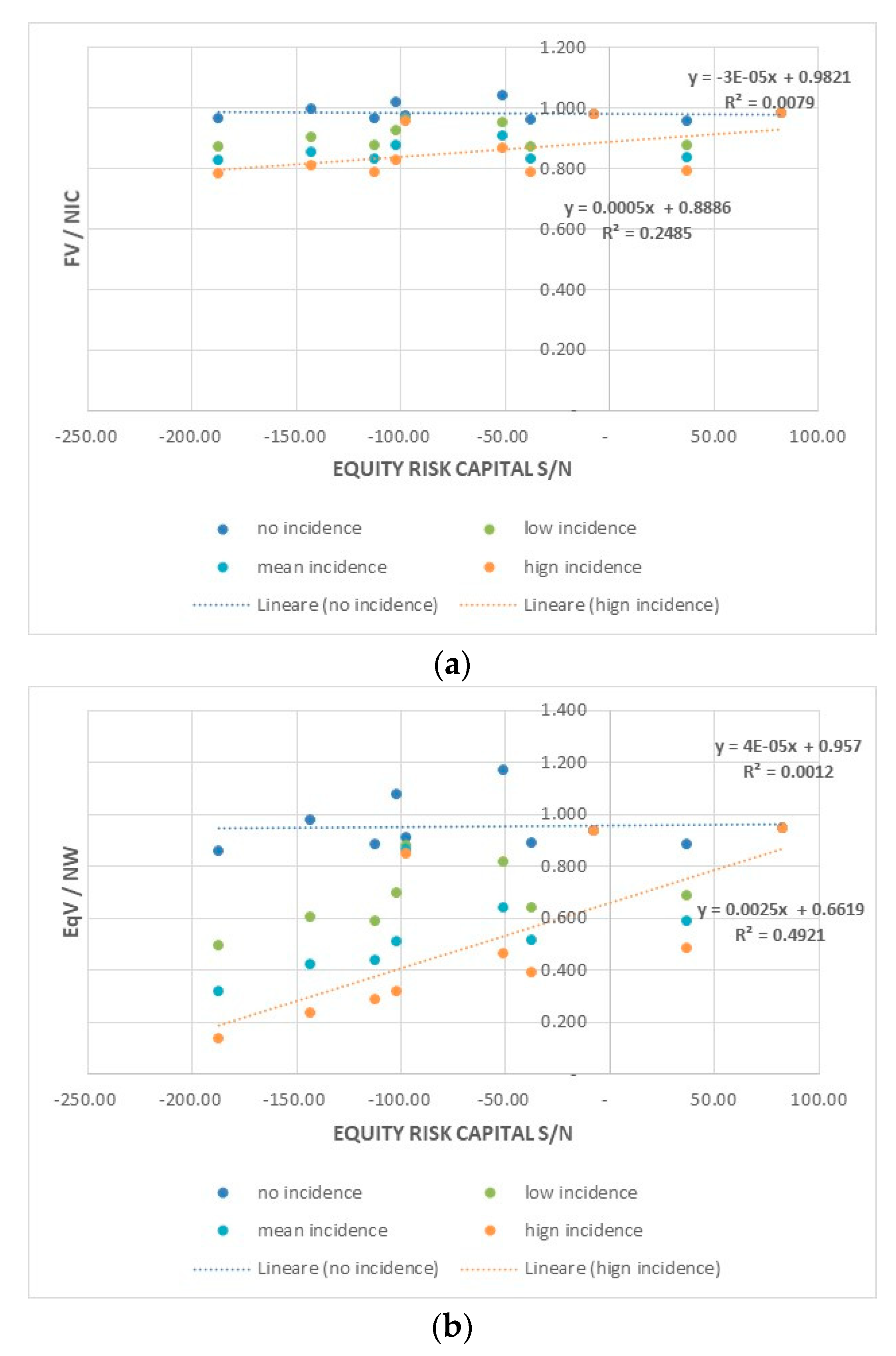
If the costs of default have a relevant (medium or high) incidence, the multiples implicit in the firm value (see Figure 14a) and equity value (see Figure 14b) tend to decrease significantly as the probability of default increases.
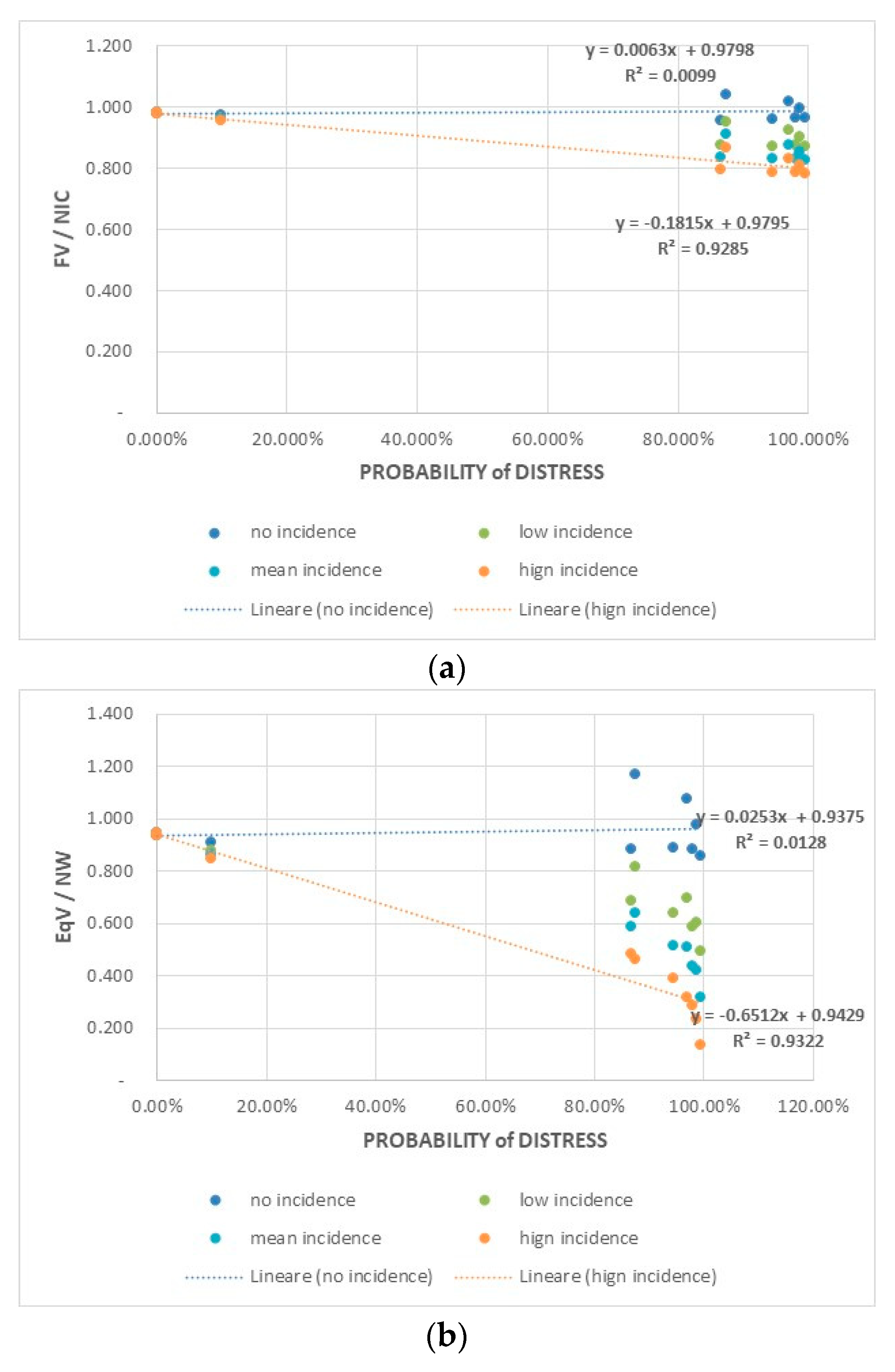
A similar behavior was observed considering the distress probability estimated in the first year of the plan; the reduction effects are significant both on asset-side (see Figure 15a) and equity-side (see Figure 15b) multiples due to the higher incidence of restructuring costs compared with bankruptcy costs.
In other words, the insolvency costs reduce the firm value consistently with the trade-off theory on the one hand, and on the other eliminate the advantage for shareholders deriving from the asymmetry of the firm’s payoffs, consistently with the option pricing model.
The simulation model also allows us to depict the dynamics of firm value and equity value compared to the risk-capital excess or deficit. Moving from a situation of an ERC deficit to a surplus one, the value creation increases, both on the asset side (see Figure 16a) and the equity side (see Figure 16b), only if the default costs are significant.
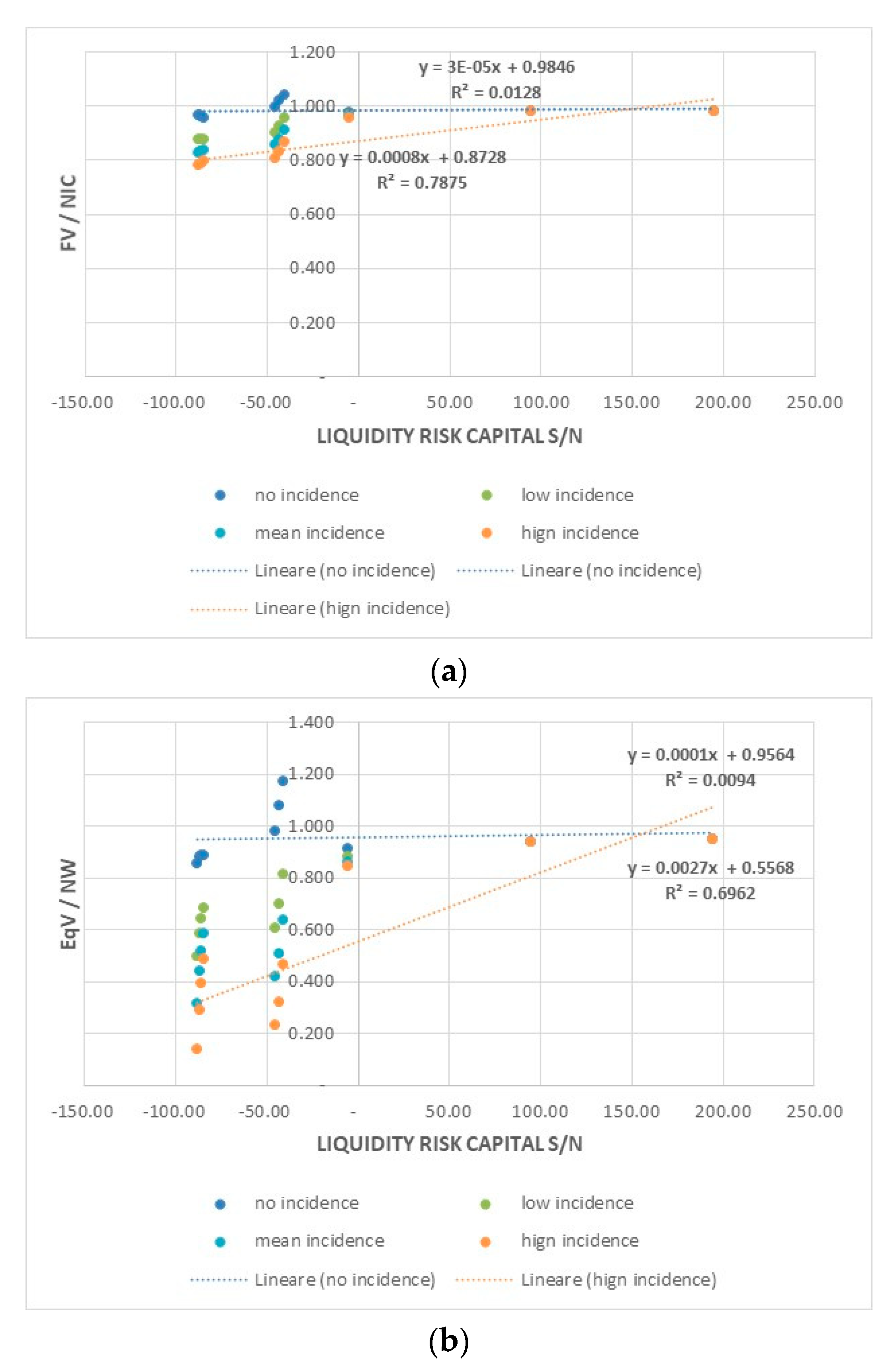
Without insolvency costs, surpluses or needs of equity capital have almost zero effects on firm value and equity value. The ERC is therefore useful to detect excessive default risk hedging, incoherent with the principle of shareholder value creation. When insolvency costs become relevant, an excess of equity capital benefits the value creation for shareholders and lenders. Similar considerations apply to the correlation between asset multiples (see Figure 17a) or equity multiples (see Figure 17b) and deficits/excesses of liquidity risk-capital.
Therefore, risk-capital measures are useful in defining financial policies aimed at reducing the insolvency risk consistently with the principle of corporate value maximization. When insolvency costs are null, excesses of equity or liquidity generate negative effects on firm value. This is due to an excess of assets less profitable than the operating ones and a financial debt not sufficient to fully obtain the potential tax benefits. When insolvency costs become relevant, an excess of equity or liquidity might help to create value for all investors (shareholders and lenders) depending on the magnitude of those costs.
6. Conclusions
This paper aims to:
- (1)
- define and quantify risk-based capital measures to counter the insolvency risk in non-financial companies;
- (2)
- investigate conditions on and limits to their use in financing strategies.
(1). Two risk-capital measures were proposed. Equity risk-capital us allows to check whether the financial structure presents a net worth sufficient to ensure the “medium to long term solvency” of the firm; liquidity risk-capital allows us to check whether the firm has sufficient liquidity to balance cash in and cash out, ensuring “short-term solvency”. These risk capital measures depend on the operating cash flow variability—due to competitive strategies and operating policies—and on capital structure—determined by the firm financing policies. Corporate policies determine the asset and cost structure of a firm and, therefore, the way in which the uncertainty of turnover becomes the variability in its operating results; financing policies determine the firm’s ability to cover financial needs. Consequently, the nature of the firm (manufacturing, commercial, service company), the industry to which it belongs, and the investments done (development or maintenance) affect both the LRC and ERC.
These measures are based on the VaR logic and require a simulation approach to financial planning and budgeting. The simulation model allows us to explicitly consider the variability in the expected returns in financial plans and budgets. Although advanced tools and models for data analysis and forecasting have been developed thanks to technological and digital innovation, their use by CFOs remains relatively limited, especially in SMEs. Both of the proposed measures depend on several choices that management should make to apply the VaR logic and to set up forecasting procedures for planning and budgeting. These choices have a relevant impact on the estimation of the proposed risk-capital measures, which are strictly dependent on the management approach to risk assessment and forecasting.
(2). The simulation model allows us to check whether a firm’s financial policies, based on a reduction in LRC or ERC needs/surplus and aimed at reducing the insolvency risk, are consistent with the principle of corporate value maximization. The main results from the simulation model are as follows.
A corporate capital structure optimization based on LRC and ERC gives benefits in terms of value maximization. When the insolvency costs are relevant, consistently with the trade-off theory, ERC and LRC are useful to balance the advantages (tax benefits) and disadvantages (direct and indirect costs of bankruptcy) of a financial policy.
Practical implications in the entrepreneurial and managerial field are evident.
A firm should consider LRC or ERC as “theoretical” or “regulatory” measures useful to implement capital structures (assets and liabilities) able to maintain conditions of financial equilibrium in the short and medium to long term. Therefore, the proposed risk-capital measures are useful to compose a decision-making model for corporate financial policies that integrates the goals of value maximization and equilibrium maintenance and allows for a continuous assessment of the trade-off between insolvency risk and firm value.
LRC allows for an assessment of the debt reserves and, therefore, of the effective financial flexibility of the firm. Debt reserves built with lines of credit linked to operations’ volume or turnover do not always allow for the elimination of the risk of financial distress. This is because they may be not available or may generate mandatory repayments that increase the lack of liquidity.
Since the costs of financial default are normally significant, both direct (restructuring procedures) and indirect (loss of market and margins), LRC and ERC appear useful in preventing and facing corporate financial crises, allowing for an assessment of default probability and financial buffers. These measures make it possible to compose growth or turnaround strategies based on the full sustainability, within a certain level of confidence, of future financial policies.
Although LRC and ERC are effective measures for quantifying the capital buffers necessary to counter insolvency risk, this paper presents just the first step of the search for a full convergence between risk management and financial management. The main limits of the results discussed above relate to the approach in defining the main parameters of the simulation model (growth rate, variable costs, interest rates, etc.). This approach does not incorporate into the simulation processes the (limited) ability of companies to adapt their financial strategies and policies to the competitive pressures and dynamics of the context. Nevertheless, to have a more comprehensive analysis and to provide more confidence in the simulation’s results, future research will include: considering alternative probability distributions (beta, log-normal, etc.) for turnover and the interest rate; designing an effective methodology to perform an empirical check of LRC and ERC, first through case studies and then though an econometric analysis; and verifying whether the use of LRC and ERC in financial strategies allows us to improve the risk profile perceived by financial investors and intermediaries.
Funding
This research received no external funding.
Institutional Review Board Statement
Not applicable.
Informed Consent Statement
Not applicable.
Data Availability Statement
Not applicable.
Conflicts of Interest
The authors declare no conflict of interest.
References
- Alviniussen, Alf, and Hakan Jankensgard. 2009. Enterprise Risk Budgeting—Bringing Risk Management into the Financial Planning Process. Journal of Applied Finance 19: 178–92. [Google Scholar]
- Andersen, Torben Juul, and Oliviero Roggi. 2012. Strategic Risk Management and Corporate Value Creation. In Annual International Conference of Strategic Management Society. Paper presented at 32nd Annual International Conference, Prague, Czech Republic, October 7–9. [Google Scholar]
- Andren, Niclas, Håkan Jankensgård, and Lars Oxelheim. 2005. Exposure-based Cash-Flow-at-Risk: An Alternative to Value-at-Risk for Industrial Companies. Journal of Applied Corporate Finance 17: 76–86. [Google Scholar] [CrossRef]
- Appiah, Kingsley Opoku, Amon Chizema, and Joseph Arthur. 2015. Predicting corporate failure: a systematic literature review of methodological issues. International Journal of Law and Management 57: 461–85. [Google Scholar] [CrossRef]
- Barbuta-Misu, Nicoleta, and Mara Madaleno. 2020. Assessment of Bankruptcy Risk of Large Companies: European Countries Evolution Analysis. Journal of Risk and Financial Management 13: 58. [Google Scholar] [CrossRef]
- Black, Fischer, and Myros Scholes. 1973. The Pricing of Options and Corporate Liabilities. Journal of Political Economy 81: 637–54. [Google Scholar] [CrossRef] [Green Version]
- Conti, Cesare. 2006. Introduzione al Corporate Financial Risk Management. Una Chiave di Lettura Finanziaria per il Board. Milano: Pearson. [Google Scholar]
- Copeland, Thomas E., John Fred Weston, and Kuldeep Shastri. 2005. Financial Theory and Corporate Policy. Boston: Pearson Addison Wesley. [Google Scholar]
- Culp, Christopher L. 2002. Contingent capital: integrating corporate financing and risk management decisions. Journal of Applied Corporate Finance 15: 46–56. [Google Scholar] [CrossRef]
- Damodaran, Aswath. 2006. The Cost of Distress: Survival, Truncation Risk and Valuation. Available online: https://ssrn.com/abstract=887129 (accessed on 1 January 2006).
- Doherty, Neil. 2005. Risk Management, Risk Capital, and the Cost of Capital. Journal of Applied Corporate Finance 17: 119–23. [Google Scholar] [CrossRef]
- Falkner, Eva Maria, and Martin R. W. Hiebl. 2015. Risk Management in SMEs: A Systematic Review of Available Evidence. Journal of Risk Finance 16: 122–44. [Google Scholar] [CrossRef]
- Farooq, Umar, and Ali Qamar Jibran. 2018. Scope, measurement, impact size and determinants of indirect cost of financial distress: A systematic literature review. Qualitative Research in Financial Markets 10: 111–29. [Google Scholar] [CrossRef]
- Forestieri, Giancarlo, and Paolo Maria Mottura. 2013. Il Sistema Finanziario. Milano: Egea. [Google Scholar]
- Froot, Kenneth A., David S. Scharfstein, and Jeremy C. Stein. 1993. Risk Management: Coordinating Investment and Financing Policies. Journal of Finance 48: 1629–58. [Google Scholar] [CrossRef] [Green Version]
- Graham, John R., and Mark T. Leary. 2018. The Evolution of Corporate Cash. Journal of Applied Corporate Finance 31: 4288–344. [Google Scholar]
- Harris, Christopher, and Scott Roark. 2018. Cash flow risk and capital structure decisions. Finance Research Letters 29: 393–97. [Google Scholar] [CrossRef]
- Hertz, David B. 1964. Risk Analysis in Capital Investment. Harvard Business Review 42: 95–106. [Google Scholar]
- Hertz, David B. 1968. Investment Policies that Pay Off. Harvard Business Review 46: 96–108. [Google Scholar]
- Hull, John C. 2018. Risk Management and Financial Institutions, 5th ed. New York: John Wiley & Sons. [Google Scholar]
- Jankensgard, Håkan. 2008. Cash Flow-at-Risk and Debt Capacity. Available online: https://ssrn.com/abstract=1304108 (accessed on 19 November 2008).
- Koh, SzeKee, Robert B. Durand, Lele Dai, and Millicent Chang. 2015. Financial Distress: Lifecycle and Corporate Restructuring. Journal of Corporate Finance 33: 19–33. [Google Scholar] [CrossRef] [Green Version]
- Leland, Hayne E. 1998. Agency Costs, Risk Management, and Capital Structure. The Journal of Finance 53: 1213–43. [Google Scholar] [CrossRef]
- Magerakis, Efstathios, Konstantinos Gkillas, Athanasios Tsagkanos, and Costas Siriopoulos. 2020. Firm Size Does Matter: New Evidence on the Determinants of Cash Holdings. Journal of Risk and Financial Management 13: 163. [Google Scholar] [CrossRef]
- Merton, Robert C. 1974. On the Pricing of Corporate Debt: The Risk Structure of Interest Rates. The Journal of Finance 29: 449–70. [Google Scholar]
- Merton, Robert. 2005. You Have More Capital Than You Think. Harward Business Review 83: 84. [Google Scholar]
- Merton, Robert C., and Andre F. Perold. 1993. Theory of Risk Capital in Financial Firms. Journal of Applied Corporate Finance 6: 131–61. [Google Scholar] [CrossRef]
- Modigliani, Franco, and Merton H. Miller. 1958. The Cost of Capital, Corporation Finance and the Theory of Investment. American Economic Review 48: 261–97. [Google Scholar]
- Modigliani, Franco, and Merton H. Miller. 1963. Corporate Income Taxes and the Cost of Capital: a Correction. American Economic Review 53: 433–43. [Google Scholar]
- Nawrocki, David. 1999. A Brief History of Downside Risk Measures. Journal of Investing 8: 9–25. [Google Scholar] [CrossRef] [Green Version]
- Newton, Grant W. 2009. Bankruptcy and Insolvency Accounting (Vol. I). Hoboken: John Wiley & Sons. [Google Scholar]
- Nikolov, Boris, Lukas Schmid, and Roberto Steri. 2019. Dynamic corporate liquidity. Journal of Financial Economics 132: 76–102. [Google Scholar] [CrossRef]
- Nocco, Brian W., and René M. Stulz. 2006. Enterprise Risk Management: Theory and Practice. Journal of Applied Corporate Finance 18: 8–20. [Google Scholar] [CrossRef]
- O’Brien, Thomas J. 2006. Risk Management and the Cost of Capital for Operating Assets. Journal of Applied Corporate Finance 18: 105–9. [Google Scholar] [CrossRef]
- Palazzo, Berardino. 2019. Cash flows risk, capital structure, and corporate bond yields. Annals of Finance 15: 401–20. [Google Scholar] [CrossRef]
- RiskMetrics. 1999. CorporateMetricsTM Technical Document. New York: RiskMetrics Group. [Google Scholar]
- Roggi, Oliviero. 2016. Risk, Value and Default—World Scientific Series in Finance, Vol. 8. Singapore: World Scientific Publishing. [Google Scholar]
- Ross, Stephen A., Randolph W. Westerfield, and Jeffrey Jaffe. 2013. Corporate Finance, 10th ed. New York: McGraw-Hill/Irvin. [Google Scholar]
- Shi, Yin, and Xiaoni Li. 2019. An overview of bankruptcy prediction models for corporate firms: A systematic literature review. Intangible Capital 15: 114–27. [Google Scholar] [CrossRef] [Green Version]
- Stein, Jeremy C., Stephen E. Usher, Daniel LaGattuta, and Jeff Youngen. 2001. A Comparables Approach to Measuring Cash flow-at-Risk for Non-Financial Firms. Journal of Applied Corporate Finance 13: 100–9. [Google Scholar] [CrossRef]
- Wieczorek-Komsala, Monika. 2019. The Concept of Risk Capital and Its Application in Non-Financial Companies: A Sustainable Dimension. Sustainability 11: 894. [Google Scholar] [CrossRef] [Green Version]
Figure 1.
Probabilistic distribution of the first year growth rate.

Figure 2.
Main ratios: (a) Financial leverage changes. (b) Dynamic of Roe.

Figure 3.
Probabilistic distributions of FVgc and areas of default risk.

Figure 4.
Probabilistic distributions of FVlc and areas of bankruptcy risk.
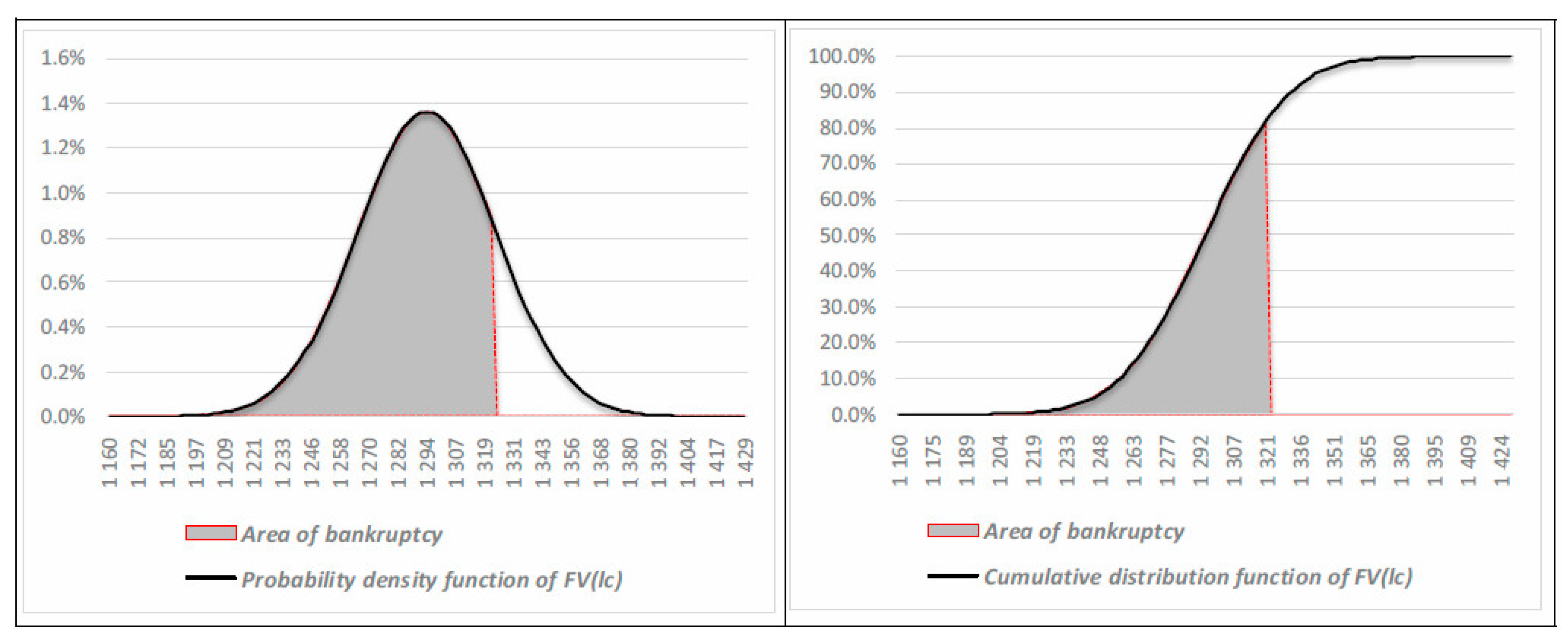
Figure 5.
Probabilistic distributions of CFF and FSN: (a) March. (b) May.

Figure 6.
Monthly cash flows and risks: (a) Expected cash flows. (b) Distress probabilities.
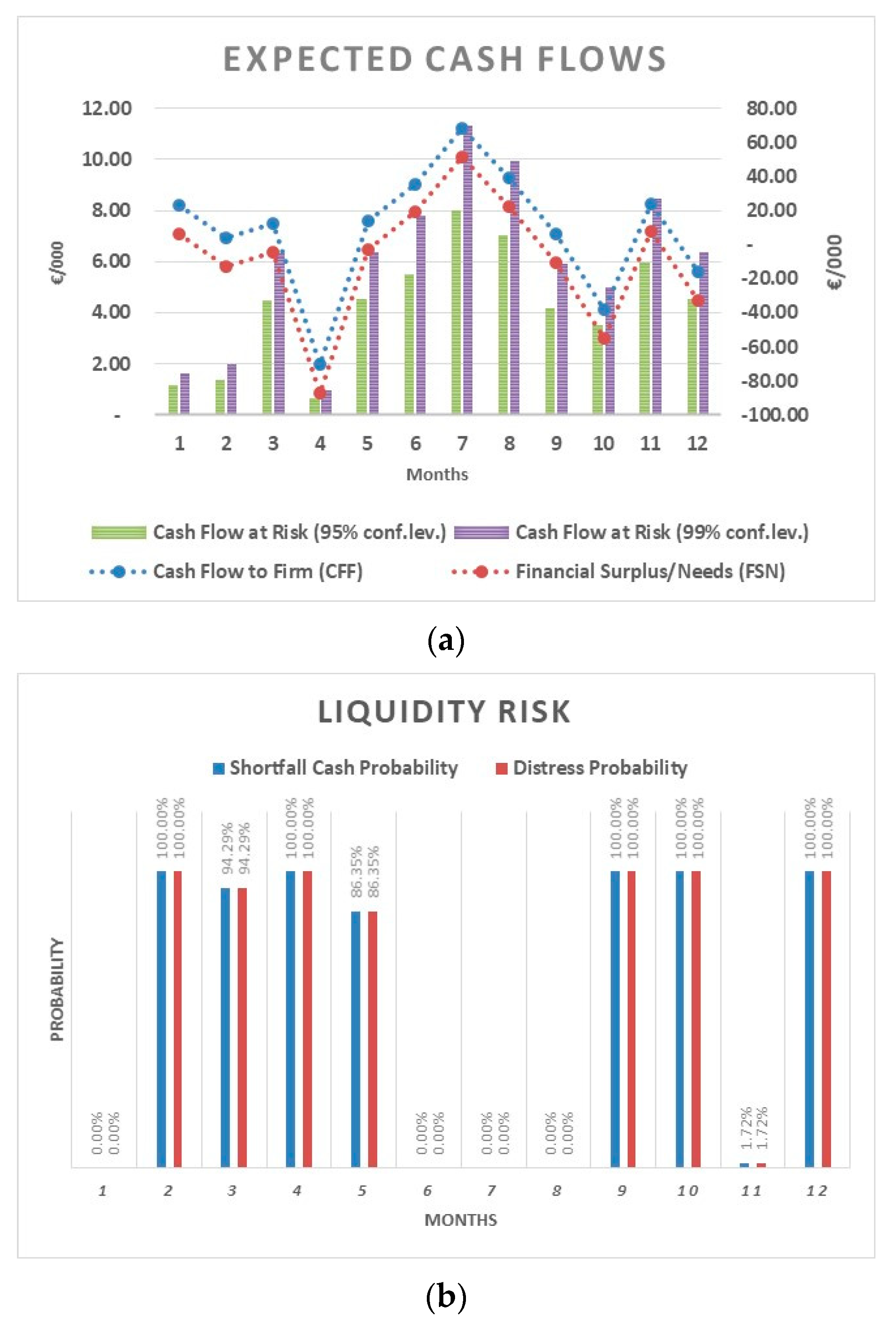
Figure 7.
Liquidity Risk Capital: (a) Risk Capital Surplus/Needs and Resilience Index. (b) Optimal and Available Liquidity Risk Capital.
Figure 7.
Liquidity Risk Capital: (a) Risk Capital Surplus/Needs and Resilience Index. (b) Optimal and Available Liquidity Risk Capital.

Figure 8.
First simulation: dynamics of capital structure, risk and value: (a) Debt/equity ratio. (b) Equity risk capital. (c) Insolvency risk. (d) Value creation.
Figure 8.
First simulation: dynamics of capital structure, risk and value: (a) Debt/equity ratio. (b) Equity risk capital. (c) Insolvency risk. (d) Value creation.


Figure 9.
First simulation: dynamics of Liquidity Risk Capital: (a) Optimal liquidity risk-capital. (b) Available liquidity risk-capital. (c) Shortfall in cash risk. (d) Distress probability.
Figure 9.
First simulation: dynamics of Liquidity Risk Capital: (a) Optimal liquidity risk-capital. (b) Available liquidity risk-capital. (c) Shortfall in cash risk. (d) Distress probability.
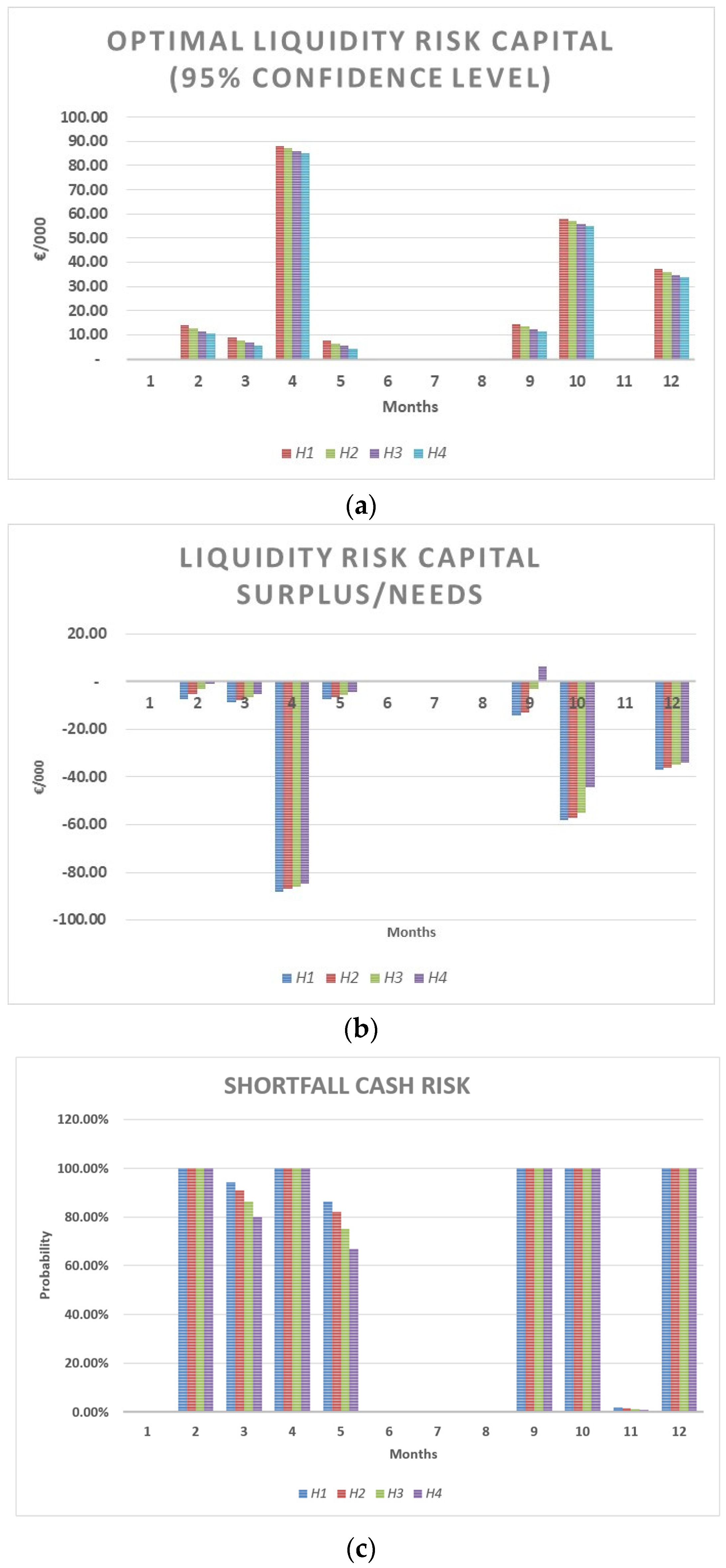

Figure 10.
Second simulation: dynamics of capital structure, risk and value: (a) Debt/equity ratio. (b) Equity risk capital. (c) Insolvency risk. (d) Value creation.
Figure 10.
Second simulation: dynamics of capital structure, risk and value: (a) Debt/equity ratio. (b) Equity risk capital. (c) Insolvency risk. (d) Value creation.
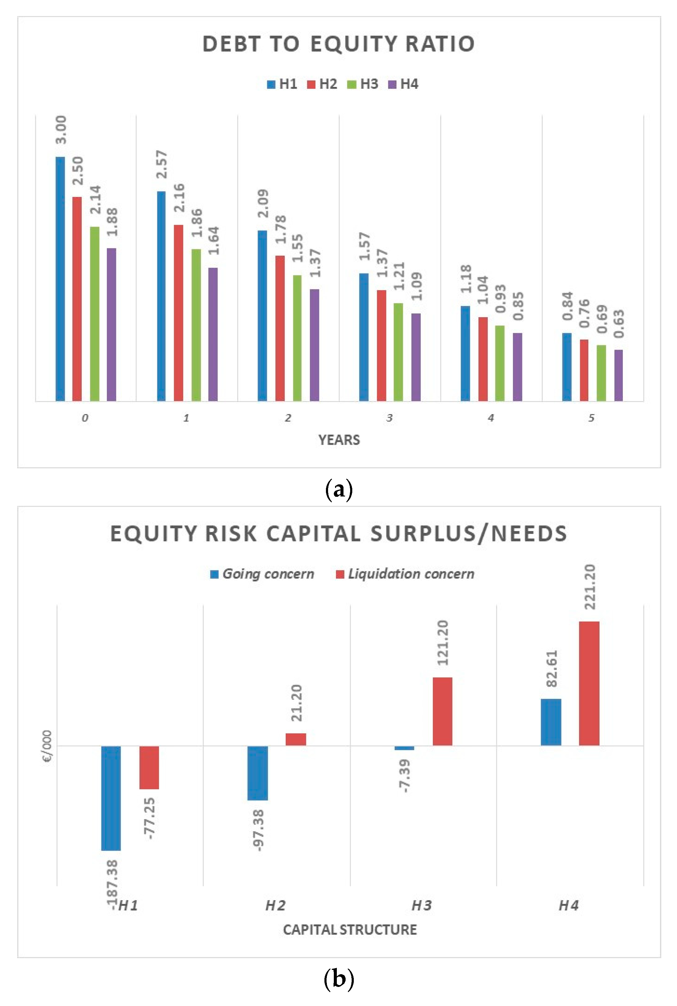

Figure 11.
Second simulation: dynamics of Liquidity Risk Capital: (a) Optimal liquidity risk-capital. (b) Available liquidity risk-capital. (c) Shortfall in cash risk. (d) Distress probability.
Figure 11.
Second simulation: dynamics of Liquidity Risk Capital: (a) Optimal liquidity risk-capital. (b) Available liquidity risk-capital. (c) Shortfall in cash risk. (d) Distress probability.


Figure 12.
Third simulation: dynamics of capital structure, risk and value: (a) Short-term debt. (b) Equity risk capital. (c) Insolvency risk. (d) Value creation.
Figure 12.
Third simulation: dynamics of capital structure, risk and value: (a) Short-term debt. (b) Equity risk capital. (c) Insolvency risk. (d) Value creation.


Figure 13.
Third simulation: dynamics of Liquidity Risk Capital: (a) Optimal liquidity risk-capital. (b) Available liquidity risk-capital. (c) Shortfall in cash risk. (d) Distress probability.
Figure 13.
Third simulation: dynamics of Liquidity Risk Capital: (a) Optimal liquidity risk-capital. (b) Available liquidity risk-capital. (c) Shortfall in cash risk. (d) Distress probability.


Figure 14.
Multiples and probability of default: (a) Asset multiples. (b) Equity multiples.


Figure 15.
Multiples and probability of distress: (a) Asset multiples. (b) Equity multiples.

Figure 16.
Multiples and Equity Risk Capital: (a) Asset multiples and Equity Risk Capital surplus/needs. (b) Equity multiples and Equity Risk Capital surplus/needs.
Figure 16.
Multiples and Equity Risk Capital: (a) Asset multiples and Equity Risk Capital surplus/needs. (b) Equity multiples and Equity Risk Capital surplus/needs.

Figure 17.
Multiples and Liquidity Risk Capital: (a) Asset multiples and Liquidity Risk Capital surplus/needs. (b) Equity multiples and Liquidity Risk Capital surplus/needs.
Figure 17.
Multiples and Liquidity Risk Capital: (a) Asset multiples and Liquidity Risk Capital surplus/needs. (b) Equity multiples and Liquidity Risk Capital surplus/needs.


Table 1.
Liquidity Risk Capital and implicit probability of financial distress.
| Risk Capital | Probability of Financial Distress |
|---|---|
Table 2.
Equity Risk Capital and implicit probability of default.
| Risk Capital in a Going Concern | Probability of Default |
|---|---|
Table 3.
Equity Risk Capital and implicit probability of bankruptcy.
| Risk Capital in a Liquidation Concern | Probability of Bankruptcy |
|---|---|
Table 4.
Annual growth rate of revenues in alternative scenarios.
| Years | ||||||
|---|---|---|---|---|---|---|
| Growth Rates | 1 | 2 | 3 | 4 | 5 | LTGR |
| Expected | 2.0% | 4.0% | 4.0% | 3.0% | 1.0% | 1.0% |
| Standard Deviation | 3.0% | 3.0% | 3.0% | 3.0% | 3.0% | 3.0% |
Table 5.
Seasonality of annual revenues.
| Seasonality | |||||||||||||
|---|---|---|---|---|---|---|---|---|---|---|---|---|---|
| Months | 1 | 2 | 3 | 4 | 5 | 6 | 7 | 8 | 9 | 10 | 11 | 12 | FY |
| Expected | 8% | 5% | 10% | 11% | 12% | 10% | 8% | 6% | 9% | 7% | 8% | 6% | 100% |
Table 6.
Expected results: (a) Expected earnings at end of year 1. (b) Expected cash flows at end of year 1.
Table 6.
Expected results: (a) Expected earnings at end of year 1. (b) Expected cash flows at end of year 1.
| (a) | ||||||
| P/L (k/€) | Forecasts | |||||
| Scenario | 1 | 2 | … | 15 | E | Sd |
| Probabilities | 0.91% | 1.82% | … | 0.91% | ||
| Revenues | 1710.00 | 1728.00 | … | 1962.00 | 1832.92 | 50.91 |
| Variable costs | −342.00 | −345.60 | … | −392.40 | −366.58 | 10.18 |
| Fixed costs | −1200.00 | −1200.00 | … | −1200.00 | −1200.00 | 0.00 |
| EBITDA | 168.00 | 182.40 | … | 369.60 | 266.33 | 40.72 |
| Depr. and Amort. | −181.10 | −181.10 | … | −181.10 | −181.10 | 0.00 |
| EBIT | −13.10 | 1.30 | … | 188.50 | 85.23 | 40.72 |
| Interest on Bonds | −52.50 | −52.50 | … | −52.50 | −52.50 | 0.00 |
| Interest on Loans | 0.00 | 0.00 | … | 0.00 | 0.00 | 0.00 |
| EBT | −65.60 | −51.20 | … | 136.00 | 32.73 | 40.72 |
| Taxes | 0.00 | 0.00 | … | −34.00 | −8.18 | 8.53 |
| NI | −65.60 | −51.20 | … | 102.00 | 24.55 | 32.69 |
| (b) | ||||||
| CASH FLOW STAT. (k/€) | Forecasts | |||||
| Scenario | 1 | 2 | … | 15 | E | Sd |
| Cash In Flow | 1776.30 | 1791.84 | … | 1993.86 | 1882.42 | 43.95 |
| Cash Out Flow | −1533.62 | −1537.02 | … | −1615.16 | −1564.99 | 17.92 |
| Operating Cash Flow (CFO) | 242.68 | 254.82 | … | 378.70 | 317.43 | 26.33 |
| Cap.Ex. | −181.10 | −181.10 | … | −181.10 | −181.10 | 0.00 |
| CASH FLOW to FIRM (CFF) | 61.58 | 73.72 | … | 197.60 | 136.33 | 26.33 |
| Interest on Bonds | −52.50 | −52.50 | … | −52.50 | −52.50 | 0.00 |
| Interest on Loans | 0.00 | 0.00 | … | 0.00 | 0.00 | 0.00 |
| Repayments on Bonds | −150.00 | −150.00 | … | −150.00 | −150.00 | 0.00 |
| Mandatory repayments on Loans (ARF) | 0.00 | 0.00 | … | 0.00 | 0.00 | 0.00 |
| FINANCIAL SURPLUS/(NEEDS) | −140.92 | −128.78 | … | −4.90 | −66.17 | 26.33 |
| Uses of ARF | 0.00 | 0.00 | … | 0.00 | 0.00 | 0.00 |
| Uses of LoF | 0.00 | 0.00 | … | 0.00 | 0.00 | 0.00 |
| FREE CASH FLOW to EQUITY (FCFE) | −140.92 | −128.78 | … | −4.90 | −66.17 | 26.33 |
| Discretional repayments on Loans (ARF) | 0.00 | 0.00 | … | 0.00 | 0.00 | 0.00 |
| Discretional repayments on Loans (LoC) | 0.00 | 0.00 | … | 0.00 | 0.00 | 0.00 |
| Dividend pay-out | 0.00 | 0.00 | … | 0.00 | 0.00 | 0.00 |
| NET CASH FLOW (NCF) | −140.92 | −128.78 | … | −4.90 | −66.17 | 26.33 |
Table 7.
Expected economic and liquidation values.
| FIRM VALUATION (t = 0; k/€) | Scenario | |||||
|---|---|---|---|---|---|---|
| Economic Values | 1 | 2 | … | 15 | E | Sd |
| Probabilities | 0.91% | 1.82% | … | 0.91% | ||
| ECONOMIC ASSET VALUE | 677.48 | 833.12 | … | 2766.04 | 1698.36 | 419.35 |
| CASH & CASH EQUIVALENT | 0.00 | 0.00 | … | 0.00 | 0.00 | 0.00 |
| TAX SHIELD | 291.98 | 291.98 | … | 315.69 | 312.28 | 6.87 |
| FVgc | 969.46 | 1125.10 | … | 3081.73 | 2010.64 | 424.37 |
| FD | −1500.00 | −1500.00 | … | −1500.00 | −1500.00 | 0.00 |
| EqVgc | −530.54 | −374.90 | … | 1581.73 | 510.64 | 424.37 |
| FV/CINactual | 0.48 | 0.56 | … | 1.54 | 1.01 | 0.21 |
| EqV/NWactual | −1.06 | −0.75 | … | 3.16 | 1.02 | 0.85 |
| FVlc | 1213.89 | 1227.05 | … | 1364.70 | 1294.47 | 29.30 |
| EqVlc | −109.64 | −96.48 | … | 41.17 | −29.06 | 29.30 |
| FV/CINactual | 0.61 | 0.61 | … | 0.68 | 0.65 | 0.01 |
| EqV/NWactual | −0.22 | −0.19 | … | 0.08 | −0.06 | 0.06 |
Table 8.
Risk-based measures for default and bankruptcy risk.
| Confidence Level | Confidence Level | |||||
|---|---|---|---|---|---|---|
| Expected Value | E | SD | 95.00% | CaR | 99.00% | CaR |
| FVgc | 2010.64 | 424.37 | 1312.62 | 698.02 | 1023.42 | 987.23 |
| FVlc | 1294.47 | 29.30 | 1246.27 | 48.20 | 1226.31 | 68.17 |
| Expected Value | Threshold | ERC | ARC | RCn/s | ARC | RCn/s |
| FVgc | 1500.00 | 687.38 | 500.00 | −187.38 | 500.00 | −476.58 |
| FVlc | 1323.53 | 577.25 | 500.00 | −77.25 | 500.00 | −97.22 |
Table 9.
Alternative financing strategies and financial leverages.
| Capital Structure | |||||
|---|---|---|---|---|---|
| Financing | Financial Leverage | ||||
| Strategies | H1 | H2 | H3 | H4 | |
| S1 | 75.00% | 70.00% | 65.00% | 60.00% | FD/NIC |
| 0.00% | 0.00% | 0.00% | 0.00% | FD st/FD | |
| 0.00% | 0.00% | 0.00% | 0.00% | DR/NIC | |
| 0.00% | 0.00% | 0.00% | 0.00% | C&CE/NIC | |
| S2 | 75.00% | 75.00% | 75.00% | 75.00% | FD/NIC |
| 0.00% | 0.00% | 0.00% | 0.00% | FD st/FD | |
| 0.00% | 0.00% | 0.00% | 0.00% | DR/NIC | |
| 0.00% | 5.00% | 10.00% | 15.00% | C&CE/NIC | |
| S3 | 75.00% | 75.00% | 75.00% | 75.00% | FD/NIC |
| 0.00% | 6.67% | 13.33% | 20.00% | FD st/FD | |
| 0.00% | 2.50% | 2.50% | 2.50% | DR/NIC | |
| 0.00% | 0.00% | 0.00% | 0.00% | C&CE/NIC | |
Publisher’s Note: MDPI stays neutral with regard to jurisdictional claims in published maps and institutional affiliations. |
© 2021 by the author. Licensee MDPI, Basel, Switzerland. This article is an open access article distributed under the terms and conditions of the Creative Commons Attribution (CC BY) license (https://creativecommons.org/licenses/by/4.0/).
Share and Cite
MDPI and ACS Style
Gennaro, A. Insolvency Risk and Value Maximization: A Convergence between Financial Management and Risk Management. Risks 2021, 9, 105. https://0-doi-org.brum.beds.ac.uk/10.3390/risks9060105
AMA Style
Gennaro A. Insolvency Risk and Value Maximization: A Convergence between Financial Management and Risk Management. Risks. 2021; 9(6):105. https://0-doi-org.brum.beds.ac.uk/10.3390/risks9060105
Chicago/Turabian StyleGennaro, Alessandro. 2021. "Insolvency Risk and Value Maximization: A Convergence between Financial Management and Risk Management" Risks 9, no. 6: 105. https://0-doi-org.brum.beds.ac.uk/10.3390/risks9060105
Note that from the first issue of 2016, this journal uses article numbers instead of page numbers. See further details here.